

Application of a Multispectral UAS to Assess the Cover and Biomass of the Invasive Dune Species Carpobrotus edulis
 ,
,
Abstract
:1. Introduction
2. Materials and Methods
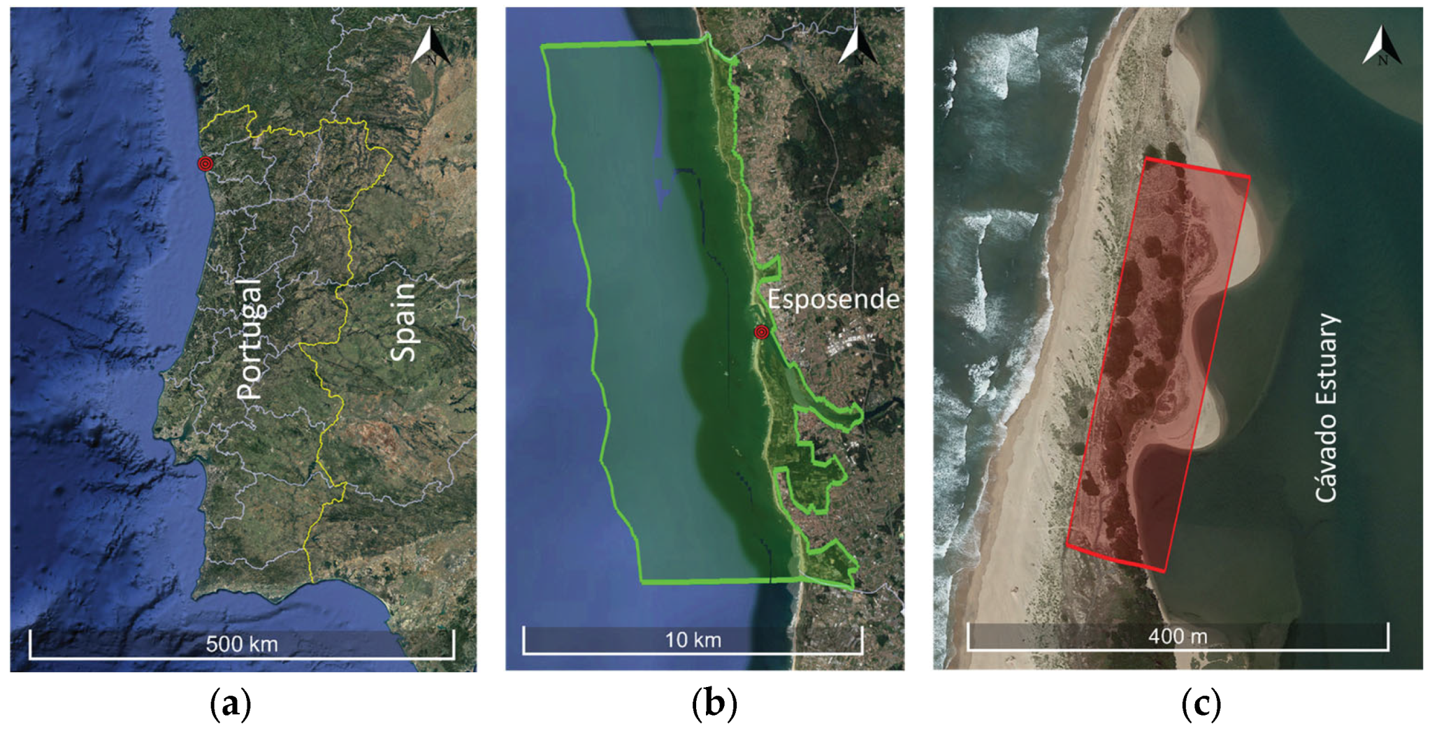
2.1. Study Area
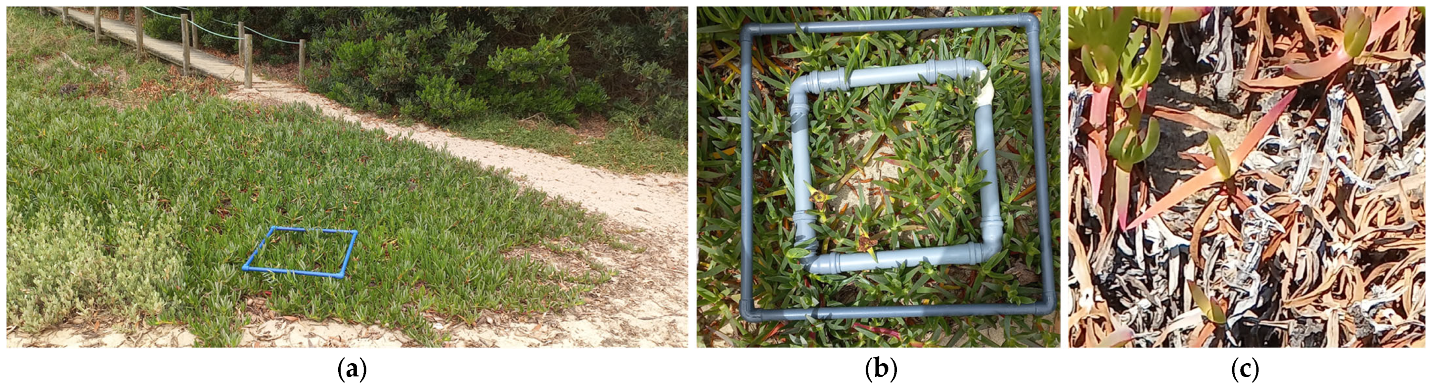
2.2. Survey and Fieldwork
2.3. Laboratory Work
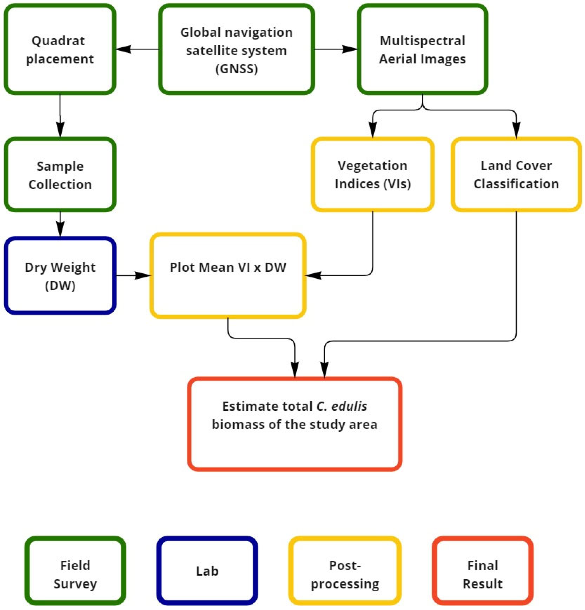
2.4. Image and Biomass Analyses
- y = Dry Weight (DW);
- x = Vegetation Index (VI);
- a = coefficient 1;
- b = coefficient 2.
- N = Number total number of pixels;
- Wi = mapped area proportion of class I;
- Si = standard deviation of stratum I;
- S0 = expected standard deviation of overall accuracy.
3. Results
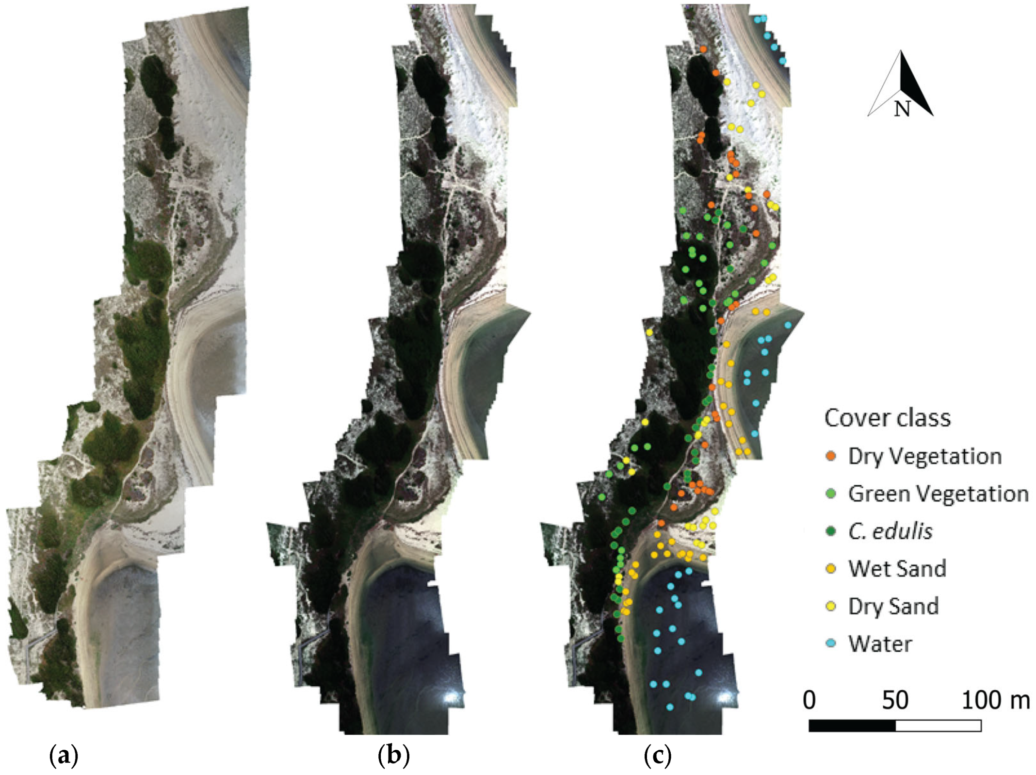
3.1. Surveys and Classification
3.2. Biomass Estimation
4. Discussion
5. Conclusions
Author Contributions
Funding
Institutional Review Board Statement
Informed Consent Statement
Data Availability Statement
Conflicts of Interest
References
- Rodríguez-Revelo, N.; Espejel, I.; García, C.A.; Ojeda-Revah, L.; Vázquez, M.A.S. Environmental Services of Beaches and Coastal Sand Dunes as a Tool for Their Conservation. In Beach Management Tools—Concepts, Methodologies and Case Studies; Botero, C.M., Cervantes, O., Finkl, C.W., Eds.; Coastal Research Library; Springer International Publishing: Cham, Switzerland, 2018; Volume 24, pp. 75–100. ISBN 978-3-319-58303-7. [Google Scholar]
- Calvão, T.; Pessoa, M.F.; Lidon, M. Impact of Human Activities on Coastal Vegetation? A Review. Emir. J. Food Agric 2013, 25, 926. [Google Scholar] [CrossRef]
- Feagin, R.A.; Furman, M.; Salgado, K.; Martinez, M.L.; Innocenti, R.A.; Eubanks, K.; Figlus, J.; Huff, T.P.; Sigren, J.; Silva, R. The Role of Beach and Sand Dune Vegetation in Mediating Wave Run up Erosion. Estuar. Coast. Shelf Sci. 2019, 219, 97–106. [Google Scholar] [CrossRef]
- Say, S.E.; Py, K. Implications of Sea Level Rise for Coastal Dune Habitat Conservation in Wales, UK. J. Coast. Conser. 2007, 11, 31–52. [Google Scholar] [CrossRef]
- Giulio, S.; Acosta, A.T.R.; Carboni, M.; Campos, J.A.; Chytrý, M.; Loidi, J.; Pergl, J.; Pyšek, P.; Isermann, M.; Janssen, J.A.M.; et al. Alien Flora across European Coastal Dunes. Appl. Veg. Sci. 2020, 23, 317–327. [Google Scholar] [CrossRef]
- Campoy, J.G.; Acosta, A.T.R.; Affre, L.; Barreiro, R.; Brundu, G.; Buisson, E.; González, L.; Lema, M.; Novoa, A.; Retuerto, R.; et al. Monographs of Invasive Plants in Europe: Carpobrotus. Bot. Lett. 2018, 165, 440–475. [Google Scholar] [CrossRef]
- Conser, C.; Connor, E.F. Assessing the Residual Effects of Carpobrotus Edulis Invasion, Implications for Restoration. Biol. Invasions 2009, 11, 349–358. [Google Scholar] [CrossRef]
- Molinari, N.; D’Antonio, C.; Thomson, G. 7 Carpobrotus as a Case Study of the Complexities of Species Impacts. In Theoretical Ecology Series; Elsevier: Amsterdam, The Netherlands, 2007; Volume 4, pp. 139–162. ISBN 978-0-12-373857-8. [Google Scholar]
- Vieites-Blanco, C.; González-Prieto, S.J. Effects of Carpobrotus Edulis Invasion on Soil Gross N Fluxes in Rocky Coastal Habitats. Sci. Total Environ. 2018, 619–620, 966–976. [Google Scholar] [CrossRef]
- Laporte-Fauret, Q.; Lubac, B.; Castelle, B.; Michalet, R.; Marieu, V.; Bombrun, L.; Launeau, P.; Giraud, M.; Normandin, C.; Rosebery, D. Classification of Atlantic Coastal Sand Dune Vegetation Using In Situ, UAV, and Airborne Hyperspectral Data. Remote Sens. 2020, 12, 2222. [Google Scholar] [CrossRef]
- Yang, C. A High-Resolution Airborne Four-Camera Imaging System for Agricultural Remote Sensing. Comput. Electron. Agric. 2012, 88, 13–24. [Google Scholar] [CrossRef]
- Magney, T.S.; Eitel, J.U.H.; Huggins, D.R.; Vierling, L.A. Proximal NDVI Derived Phenology Improves In-Season Predictions of Wheat Quantity and Quality. Agric. For. Meteorol. 2016, 217, 46–60. [Google Scholar] [CrossRef]
- Jang, G.; Kim, J.; Yu, J.-K.; Kim, H.-J.; Kim, Y.-H.; Kim, D.-W.; Kim, K.-H.; Lee, C.; Chung, Y.S. Review: Cost-Effective Unmanned Aerial Vehicle (UAV) Platform for Field Plant Breeding Application. Remote Sens. 2020, 12, 998. [Google Scholar] [CrossRef]
- Baena, S.; Moat, J.; Whaley, O.; Boyd, D.S. Identifying Species from the Air: UAVs and the Very High Resolution Challenge for Plant Conservation. PLoS ONE 2017, 12, e0188714. [Google Scholar] [CrossRef]
- Alvarez-Taboada, F.; Paredes, C.; Julián-Pelaz, J. Mapping of the Invasive Species Hakea Sericea Using Unmanned Aerial Vehicle (UAV) and WorldView-2 Imagery and an Object-Oriented Approach. Remote Sens. 2017, 9, 913. [Google Scholar] [CrossRef]
- Lopatin, J.; Dolos, K.; Kattenborn, T.; Fassnacht, F.E. How Canopy Shadow Affects Invasive Plant Species Classification in High Spatial Resolution Remote Sensing. Remote. Sens. Ecol. Conserv. 2019, 5, 302–317. [Google Scholar] [CrossRef]
- Liang, W.; Abidi, M.; Carrasco, L.; McNelis, J.; Tran, L.; Li, Y.; Grant, J. Mapping Vegetation at Species Level with High-Resolution Multispectral and Lidar Data Over a Large Spatial Area: A Case Study with Kudzu. Remote Sens. 2020, 12, 609. [Google Scholar] [CrossRef]
- Koco, Š.; Dubravská, A.; Vilček, J.; Gruľová, D. Geospatial Approaches to Monitoring the Spread of Invasive Species of Solidago Spp. Remote Sens. 2021, 13, 4787. [Google Scholar] [CrossRef]
- Baloloy, A.B.; Blanco, A.C.; Candido, C.G.; Argamosa, R.J.L.; Dumalag, J.B.L.C.; Dimapilis, L.L.C.; Paringit, E.C. Estimation of mangrove forest aboveground biomass using multispectral bands, vegetation indices and biophysical variables derived from optical satellite imageries: Rapideye, planetscope and sentinel-2. ISPRS Ann. Photogramm. Remote Sens. Spatial Inf. Sci. 2018, 4, 29–36. [Google Scholar] [CrossRef]
- Al-lami, A.K.; Abbood, R.A.; Al Maliki, A.A.; Al-Ansari, N. Using Vegetation Indices for Monitoring the Spread of Nile Rose Plant in the Tigris River within Wasit Province, Iraq. Remote Sens. Appl. Soc. Environ. 2021, 22, 100471. [Google Scholar] [CrossRef]
- Brown, S.; Narine, L.L.; Gilbert, J. Using Airborne Lidar, Multispectral Imagery, and Field Inventory Data to Estimate Basal Area, Volume, and Aboveground Biomass in Heterogeneous Mixed Species Forests: A Case Study in Southern Alabama. Remote Sens. 2022, 14, 2708. [Google Scholar] [CrossRef]
- Gomes, P.T.; Botelho, A.A.; Soares de Carvalho, G. Sistemas dunares do litoral de Esposende; Universidade do Minho: Braga, Portugal, 2002; ISBN 978-972-9027-16-1. [Google Scholar]
- Carvalho, G.S.; Granja, H.; Gomes, P.; Loureiro, E.; Renato, H.; Ribeiro, I.; Costa, A.L. New Data and New Ideas Concerning Recent Geomorphological Changes in the NW Coastal Zone of Portugal. In Proceedings of the Littoral 2002: 6th International Symposium: The Changing Coast, Porto, Portugal, 22–26 September 2002. [Google Scholar]
- Kaufman, Y.J.; Tanre, D. Atmospherically Resistant Vegetation Index (ARVI) for EOS-MODIS. IEEE Trans. Geosci. Remote Sensing 1992, 30, 261–270. [Google Scholar] [CrossRef]
- Gitelson, A.A. Remote Estimation of Canopy Chlorophyll Content in Crops. Geophys. Res. Lett. 2005, 32, L08403. [Google Scholar] [CrossRef]
- Vincini, M.; Frazzi, E.; D’Alessio, P. A Broad-Band Leaf Chlorophyll Vegetation Index at the Canopy Scale. Precis. Agric 2008, 9, 303–319. [Google Scholar] [CrossRef]
- Richardson, A.D.; Duigan, S.P.; Berlyn, G.P. An Evaluation of Noninvasive Methods to Estimate Foliar Chlorophyll Content. New Phytol. 2002, 153, 185–194. [Google Scholar] [CrossRef]
- Rasmussen, J.; Ntakos, G.; Nielsen, J.; Svensgaard, J.; Poulsen, R.N.; Christensen, S. Are Vegetation Indices Derived from Consumer-Grade Cameras Mounted on UAVs Sufficiently Reliable for Assessing Experimental Plots? Eur. J. Agron. 2016, 74, 75–92. [Google Scholar] [CrossRef]
- Rouse, J.W.; Haas, R.H.; Deering, D.W.; Schell, J.A.; Harlan, J.C. Monitoring the Vernal Advancement and Retrogradation (Green Wave Effect) of Natural Vegetation; Great Plains Corridor; NASA: Greenbelt, MD, USA, 1973.
- Meyer, G.E.; Neto, J.C. Verification of Color Vegetation Indices for Automated Crop Imaging Applications. Comput. Electron. Agric. 2008, 63, 282–293. [Google Scholar] [CrossRef]
- Gitelson, A.A.; Kaufman, Y.J.; Merzlyak, M.N. Use of a Green Channel in Remote Sensing of Global Vegetation from EOS-MODIS. Remote Sens. Environ. 1996, 58, 289–298. [Google Scholar] [CrossRef]
- Bendig, J.; Yu, K.; Aasen, H.; Bolten, A.; Bennertz, S.; Broscheit, J.; Gnyp, M.L.; Bareth, G. Combining UAV-Based Plant Height from Crop Surface Models, Visible, and near Infrared Vegetation Indices for Biomass Monitoring in Barley. Int. J. Appl. Earth Obs. Geoinf. 2015, 39, 79–87. [Google Scholar] [CrossRef]
- Gitelson, A.; Merzlyak, M.N. Quantitative Estimation of Chlorophyll-a Using Reflectance Spectra: Experiments with Autumn Chestnut and Maple Leaves. J. Photochem. Photobiol. B Biol. 1994, 22, 247–252. [Google Scholar] [CrossRef]
- Gamon, J.A.; Peñuelas, J.; Field, C.B. A Narrow-Waveband Spectral Index That Tracks Diurnal Changes in Photosynthetic Efficiency. Remote Sens. Environ. 1992, 41, 35–44. [Google Scholar] [CrossRef]
- Roujean, J.-L.; Breon, F.-M. Estimating PAR Absorbed by Vegetation from Bidirectional Reflectance Measurements. Remote Sens. Environ. 1995, 51, 375–384. [Google Scholar] [CrossRef]
- Pearson, R.L.; Miller, L.D. Remote Mapping of Standing Crop Biomass for Estimation of the Productivity of the Shortgrass Prairie, Pawnee National Grasslands, Colorado. IBP Grassland Biome; Department of Watershed Sciences, College of Forestry and Natural Resources, Colorado State University: Fort Collins, CO, USA, 1972. [Google Scholar]
- Richards, J.A. Remote Sensing Digital Image Analysis: An Introduction; Springer: Berlin/Heidelberg, Germany, 2013; ISBN 978-3-642-30061-5. [Google Scholar]
- Kruse, F.A.; Lefkoff, A.B.; Boardman, J.W.; Heidebrecht, K.B.; Shapiro, A.T.; Barloon, P.J.; Goetz, A.F.H. The Spectral Image Processing System (SIPS)—Interactive Visualization and Analysis of Imaging Spectrometer Data. Remote Sens. Environ. 1993, 44, 145–163. [Google Scholar] [CrossRef]
- Boser, B.E.; Guyon, I.M.; Vapnik, V.N. A Training Algorithm for Optimal Margin Classifiers. In Proceedings of the Fifth Annual Workshop on Computational Learning Theory, Pittsburgh, PA, USA, 27–29 July 1992; ACM: Pittsburgh, PA, USA, July, 1992; pp. 144–152. [Google Scholar]
- Ho, T.K. Random Decision Forests. In Proceedings of the 3rd International Conference on Document Analysis and Recognition, Montreal, QC, Canada, 14–15 August 1995; IEEE Computer Society Press: Montreal, QC, Canada, 1995; Volume 1, pp. 278–282. [Google Scholar]
- Olofsson, P.; Foody, G.M.; Herold, M.; Stehman, S.V.; Woodcock, C.E.; Wulder, M.A. Good Practices for Estimating Area and Assessing Accuracy of Land Change. Remote Sens. Environ. 2014, 148, 42–57. [Google Scholar] [CrossRef]
- Gonçalves, C.; Santana, P.; Brandão, T.; Guedes, M. Automatic Detection of Acacia Longifolia Invasive Species Based on UAV-Acquired Aerial Imagery. Inf. Process. Agric. 2022, 9, 276–287. [Google Scholar] [CrossRef]
- Jianhui, L.; Dingquan, L.; Gui, Z.; Haizhou, X.; Rongliang, Z.; Wangjun, L.; Youliang, Y. Study on Extraction of Foreign Invasive Species Mikania Micrantha Based on Unmanned Aerial Vehicle (UAV) Hyperspectral Remote Sensing. In Proceedings of the Fifth Symposium on Novel Optoelectronic Detection Technology and Application, Xi’an, China, 24–26 October 2018; Yu, Q., Huang, W., He, Y., Eds.; SPIE: Xi’an, China, 2019; p. 53. [Google Scholar]
- Abeysinghe, T.; Simic Milas, A.; Arend, K.; Hohman, B.; Reil, P.; Gregory, A.; Vázquez-Ortega, A. Mapping Invasive Phragmites Australis in the Old Woman Creek Estuary Using UAV Remote Sensing and Machine Learning Classifiers. Remote Sens. 2019, 11, 1380. [Google Scholar] [CrossRef]
- Mallmann, C.L.; Zaninni, A.F.; Filho, W.P. Vegetation Index Based in Unmanned Aerial Vehicle (Uav) to Improve the Management of Invasive Plants in Protected Areas, Southern Brazil. In Proceedings of the 2020 IEEE Latin American GRSS & ISPRS Remote Sensing Conference (LAGIRS), Santiago, Chile, 22–26 March 2020; IEEE: Santiago, Chile, March, 2020; pp. 66–69. [Google Scholar]
- Santos, L.M.; Ferraz, G.A.S.; Diotto, A.V.; Barbosa, B.D.S.; Maciel, D.T.; Andrade, M.T.; Ferraz, P.F.P.; Rossi, G. Coffee Crop Coefficient Prediction as a Function of Biophysical Variables Identified from RGB UAS Images. Agron. Res. 2020, 18, 1463–1471. [Google Scholar] [CrossRef]
- Yang, S.; Hu, L.; Wu, H.; Ren, H.; Qiao, H.; Li, P.; Fan, W. Integration of Crop Growth Model and Random Forest for Winter Wheat Yield Estimation from UAV Hyperspectral Imagery. IEEE J. Sel. Top. Appl. Earth Obs. Remote Sens. 2021, 14, 6253–6269. [Google Scholar] [CrossRef]
- Li, B.; Xu, X.; Zhang, L.; Han, J.; Bian, C.; Li, G.; Liu, J.; Jin, L. Above-Ground Biomass Estimation and Yield Prediction in Potato by Using UAV-Based RGB and Hyperspectral Imaging. ISPRS J. Photogramm. Remote Sens. 2020, 162, 161–172. [Google Scholar] [CrossRef]
- Bian, C.; Shi, H.; Wu, S.; Zhang, K.; Wei, M.; Zhao, Y.; Sun, Y.; Zhuang, H.; Zhang, X.; Chen, S. Prediction of Field-Scale Wheat Yield Using Machine Learning Method and Multi-Spectral UAV Data. Remote Sens. 2022, 14, 1474. [Google Scholar] [CrossRef]
- Wengert, M.; Wijesingha, J.; Schulze-Brüninghoff, D.; Wachendorf, M.; Astor, T. Multisite and Multitemporal Grassland Yield Estimation Using UAV-Borne Hyperspectral Data. Remote Sens. 2022, 14, 2068. [Google Scholar] [CrossRef]
- Wijesingha, J.; Astor, T.; Schulze-Brüninghoff, D.; Wachendorf, M. Mapping Invasive Lupinus Polyphyllus Lindl. in Semi-Natural Grasslands Using Object-Based Image Analysis of UAV-Borne Images. PFG 2020, 88, 391–406. [Google Scholar] [CrossRef]
- Michez, A.; Piégay, H.; Jonathan, L.; Claessens, H.; Lejeune, P. Mapping of Riparian Invasive Species with Supervised Classification of Unmanned Aerial System (UAS) Imagery. Int. J. Appl. Earth Obs. Geoinf. 2016, 44, 88–94. [Google Scholar] [CrossRef]
- Papp, L.; van Leeuwen, B.; Szilassi, P.; Tobak, Z.; Szatmári, J.; Árvai, M.; Mészáros, J.; Pásztor, L. Monitoring Invasive Plant Species Using Hyperspectral Remote Sensing Data. Land 2021, 10, 29. [Google Scholar] [CrossRef]
- Sabat-Tomala, A.; Raczko, E.; Zagajewski, B. Comparison of Support Vector Machine and Random Forest Algorithms for Invasive and Expansive Species Classification Using Airborne Hyperspectral Data. Remote Sens. 2020, 12, 516. [Google Scholar] [CrossRef]
- Xue, J.; Su, B. Significant Remote Sensing Vegetation Indices: A Review of Developments and Applications. J. Sens. 2017, 2017, 1–17. [Google Scholar] [CrossRef]
- Gao, L.; Wang, X.; Johnson, B.A.; Tian, Q.; Wang, Y.; Verrelst, J.; Mu, X.; Gu, X. Remote Sensing Algorithms for Estimation of Fractional Vegetation Cover Using Pure Vegetation Index Values: A Review. ISPRS J. Photogramm. Remote Sens. 2020, 159, 364–377. [Google Scholar] [CrossRef]
- Pandey, P.C.; Anand, A.; Srivastava, P.K. Spatial Distribution of Mangrove Forest Species and Biomass Assessment Using Field Inventory and Earth Observation Hyperspectral Data. Biodivers Conserv. 2019, 28, 2143–2162. [Google Scholar] [CrossRef]
- Huang, S.; Tang, L.; Hupy, J.P.; Wang, Y.; Shao, G. A Commentary Review on the Use of Normalized Difference Vegetation Index (NDVI) in the Era of Popular Remote Sensing. J. For. Res. 2021, 32, 1–6. [Google Scholar] [CrossRef]
- Hassan, M.A.; Yang, M.; Rasheed, A.; Yang, G.; Reynolds, M.; Xia, X.; Xiao, Y.; He, Z. A Rapid Monitoring of NDVI across the Wheat Growth Cycle for Grain Yield Prediction Using a Multi-Spectral UAV Platform. Plant Sci. 2019, 282, 95–103. [Google Scholar] [CrossRef]
- Guan, S.; Fukami, K.; Matsunaka, H.; Okami, M.; Tanaka, R.; Nakano, H.; Sakai, T.; Nakano, K.; Ohdan, H.; Takahashi, K. Assessing Correlation of High-Resolution NDVI with Fertilizer Application Level and Yield of Rice and Wheat Crops Using Small UAVs. Remote Sens. 2019, 11, 112. [Google Scholar] [CrossRef]
- Tenreiro, T.R.; García-Vila, M.; Gómez, J.A.; Jiménez-Berni, J.A.; Fereres, E. Using NDVI for the Assessment of Canopy Cover in Agricultural Crops within Modelling Research. Comput. Electron. Agric. 2021, 182, 106038. [Google Scholar] [CrossRef]
- Xu, Y.; Yang, Y.; Chen, X.; Liu, Y. Bibliometric Analysis of Global NDVI Research Trends from 1985 to 2021. Remote Sens. 2022, 14, 3967. [Google Scholar] [CrossRef]
- Innangi, M.; Marzialetti, F.; Di Febbraro, M.; Acosta, A.T.R.; De Simone, W.; Frate, L.; Finizio, M.; Villalobos Perna, P.; Carranza, M.L. Coastal Dune Invaders: Integrative Mapping of Carpobrotus Sp. Pl. (Aizoaceae) Using UAVs. Remote Sens. 2023, 15, 503. [Google Scholar] [CrossRef]
- Laporte-Fauret, Q.; Marieu, V.; Castelle, B.; Michalet, R.; Bujan, S.; Rosebery, D. Low-Cost UAV for High-Resolution and Large-Scale Coastal Dune Change Monitoring Using Photogrammetry. JMSE 2019, 7, 63. [Google Scholar] [CrossRef]
- Suo, C.; McGovern, E.; Gilmer, A. Coastal Dune Vegetation Mapping Using a Multispectral Sensor Mounted on an UAS. Remote Sens. 2019, 11, 1814. [Google Scholar] [CrossRef]
- Gonçalves, G.; Andriolo, U.; Gonçalves, L.M.S.; Sobral, P.; Bessa, F. Beach Litter Survey by Drones: Mini-Review and Discussion of a Potential Standardization. Environ. Pollut. 2022, 315, 120370. [Google Scholar] [CrossRef]
- Gonçalves, G.; Andriolo, U. Operational Use of Multispectral Images for Macro-Litter Mapping and Categorization by Unmanned Aerial Vehicle. Mar. Pollut. Bull. 2022, 176, 113431. [Google Scholar] [CrossRef]


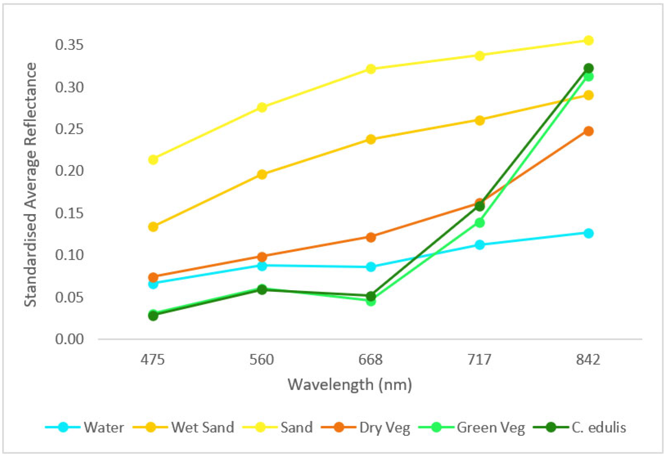
| Band | Centre Wavelength | Bandwidth |
|---|---|---|
| Blue | 475 nm | 32 nm |
| Green | 560 nm | 27 nm |
| Red | 668 nm | 16 nm |
| Red Edge | 717 nm | 12 nm |
| Near Infrared | 842nm | 57 nm |
| Index | Formula | References |
|---|---|---|
| Atmospherically Resistant Vegetation Index (ARVI) | [24] | |
| Green Chlorophyll Index (GCI) | [25] | |
| Chlorophyll Vegetation Index (CVI) | [26] | |
| Difference Vegetation Index (DVI) | [27] | |
| Green Difference Vegetation Index (GDVI) | * | |
| Enhanced Normalized Difference Vegetation Index (ENDVI) | [28] | |
| Excess Green (ExG) | [29] | |
| Excess Red (ExR) | [30] | |
| Green Normalized Difference Vegetation Index (GNDVI) | [31] | |
| Modified Green Red Vegetation Index (MGRVI) | [32] | |
| Normalized Difference Red Edge Index (NDREI) | [33] | |
| Normalized Difference Vegetation Index (NDVI) | [29] | |
| Photochemical Reflectance Index (PRI) | [34] | |
| Red–Blue difference (RB) | * | |
| Renormalized Difference Vegetation Index (RDVI) | [35] | |
| Ratio Vegetation Index (RVI) | [36] |
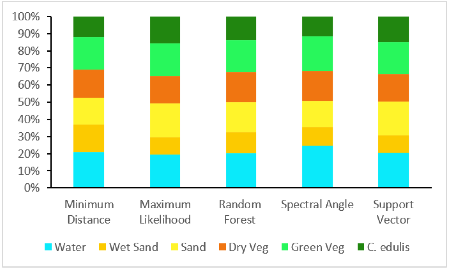
| Algorithm | C. edulis PA * | C. edulis UA * | Kappa | Overall Accuracy |
|---|---|---|---|---|
| Minimum Distance | 0.65 | 0.72 | 0.76 | 0.80 |
| Maximum Likelihood | 0.74 | 0.60 | 0.80 | 0.84 |
| Random Forest | 0.83 | 0.73 | 0.84 | 0.87 |
| Spectral Angle Mapper | 0.79 | 0.66 | 0.76 | 0.77 |
| Support Vector Machine | 0.81 | 0.67 | 0.82 | 0.85 |
| Reference | |||||||||
|---|---|---|---|---|---|---|---|---|---|
| Water | C. edulis | Sand | Wet Sand | Dry Vegetation | Green Vegetation | % Area | Total Area m2 | ||
| Classified | Water | 0.198 | 0.000 | 0.000 | 0.005 | 0.000 | 0.002 | 20.5 | 6300 |
| C. edulis | 0.000 | 0.099 | 0.000 | 0.000 | 0.004 | 0.021 | 12.4 | 3821 | |
| Sand | 0.000 | 0.002 | 0.164 | 0.006 | 0.009 | 0.000 | 18.1 | 5565 | |
| Wet Sand | 0.005 | 0.000 | 0.003 | 0.097 | 0.002 | 0.000 | 10.7 | 3279 | |
| Dry Vegetation | 0.000 | 0.002 | 0.015 | 0.006 | 0.163 | 0.017 | 20.3 | 6242 | |
| Green Vegetation | 0.000 | 0.006 | 0.000 | 0.000 | 0.006 | 0.168 | 18.0 | 5540 | |
| % Area | 20.3 | 10.9 | 18.2 | 11.4 | 18.5 | 20.8 | 100 | ||
| Total Area m2 | 6232 | 3362 | 5596 | 3497 | 5673 | 6387 | 30,748 | ||
| Standard Error m2 | 148 | 219 | 245 | 214 | 319 | 290 | |||
| Producer Accuracy | 0.98 | 0.91 | 0.90 | 0.85 | 0.88 | 0.81 | |||
| User Accuracy | 0.97 | 0.80 | 0.91 | 0.91 | 0.80 | 0.93 | |||
| Green | Brown | |||
|---|---|---|---|---|
| WW (g/m2) | DW (g/m2) | WW (g/m2) | DW (g/m2) | |
| Maximum | 27,120 | 2860 | 3650 | 2637 |
| Minimum | 1781 | 421 | 117 | 60 |
| Mean | 8912 | 1188 | 1093 | 680 |
| Median | 8035 | 1034 | 642 | 370 |
| SD | 6175 | 657 | 1052 | 687 |
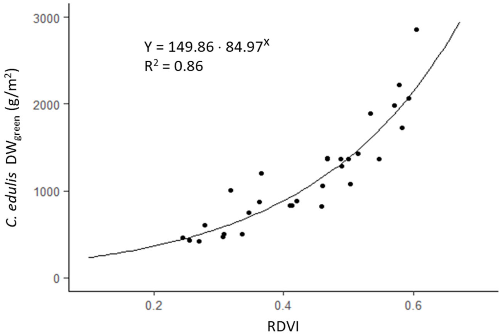
| Ranking | VI | R2 | Model |
|---|---|---|---|
| 1 | RDVI | 0.86 | |
| 2 | GDVI | 0.84 | |
| 3 | DVI | 0.84 | |
| 9 | RVI | 0.81 | |
| 10 | GCI | 0.80 | |
| 11 | ENDVI | 0.80 | |
| 12 | NDVI | 0.79 | |
| 13 | PRI | 0.79 | |
| 14 | GNDVI | 0.78 | |
| 22 | MGRVI | 0.72 | |
| 23 | ARVI | 0.71 | |
| 25 | ExR | 0.70 | |
| 33 | RB | 0.62 | |
| 34 | ExG | 0.62 | |
| 36 | NDREI | 0.59 | |
| 46 | CVI | 0.00 |
Disclaimer/Publisher’s Note: The statements, opinions and data contained in all publications are solely those of the individual author(s) and contributor(s) and not of MDPI and/or the editor(s). MDPI and/or the editor(s) disclaim responsibility for any injury to people or property resulting from any ideas, methods, instructions or products referred to in the content. |
© 2023 by the authors. Licensee MDPI, Basel, Switzerland. This article is an open access article distributed under the terms and conditions of the Creative Commons Attribution (CC BY) license (https://creativecommons.org/licenses/by/4.0/).
Share and Cite
Meyer, M.d.F.; Gonçalves, J.A.; Cunha, J.F.R.; Ramos, S.C.d.C.e.S.; Bio, A.M.F. Application of a Multispectral UAS to Assess the Cover and Biomass of the Invasive Dune Species Carpobrotus edulis. Remote Sens. 2023, 15, 2411. https://doi.org/10.3390/rs15092411
Meyer MdF, Gonçalves JA, Cunha JFR, Ramos SCdCeS, Bio AMF. Application of a Multispectral UAS to Assess the Cover and Biomass of the Invasive Dune Species Carpobrotus edulis. Remote Sensing. 2023; 15(9):2411. https://doi.org/10.3390/rs15092411
Chicago/Turabian StyleMeyer, Manuel de Figueiredo, José Alberto Gonçalves, Jacinto Fernando Ribeiro Cunha, Sandra Cristina da Costa e Silva Ramos, and Ana Maria Ferreira Bio. 2023. "Application of a Multispectral UAS to Assess the Cover and Biomass of the Invasive Dune Species Carpobrotus edulis" Remote Sensing 15, no. 9: 2411. https://doi.org/10.3390/rs15092411