
A Cross-Channel Dense Connection and Multi-Scale Dual Aggregated Attention Network for Hyperspectral Image Classification

Abstract
:1. Introduction
- (1)
- In this article, a cross channel dense connection and multi-scale dual aggregated attention network (CDC_MDAA) is proposed to alleviate the small sample problem, and extensive experiments have shown that the proposed method is superior to some state-of-the-art methods in small samples.
- (2)
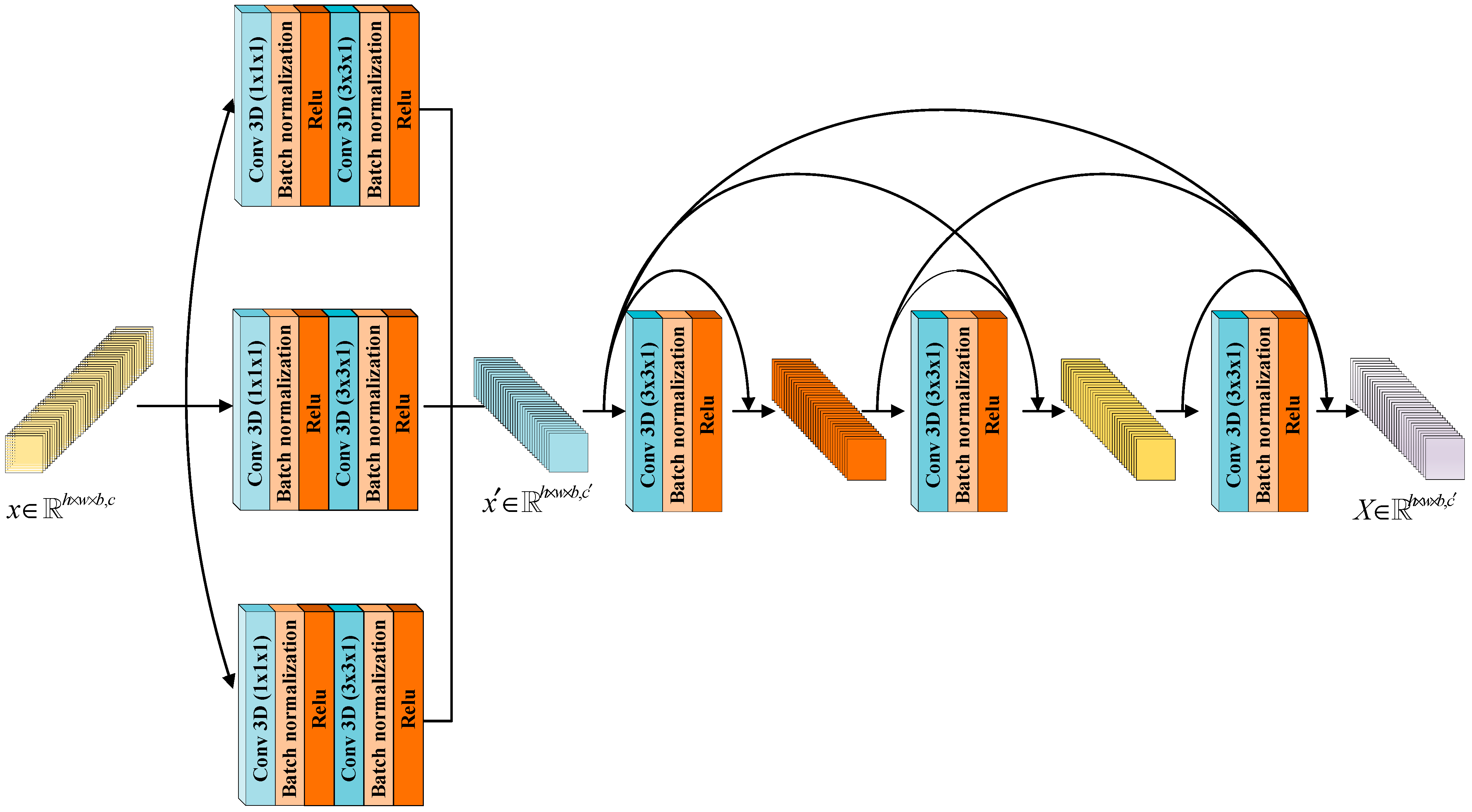
- A CDC module is proposed, which combines cross-channel convolution with dense connection to effectively extract the spatial features of HSIs. The CDC realizes the interactive fusion of channel information and introduces dense connections. The same feature can be multiplexed multiple times, the loss of information in the feature extraction process can be reduced, and too many parameters are avoided.
- (3)
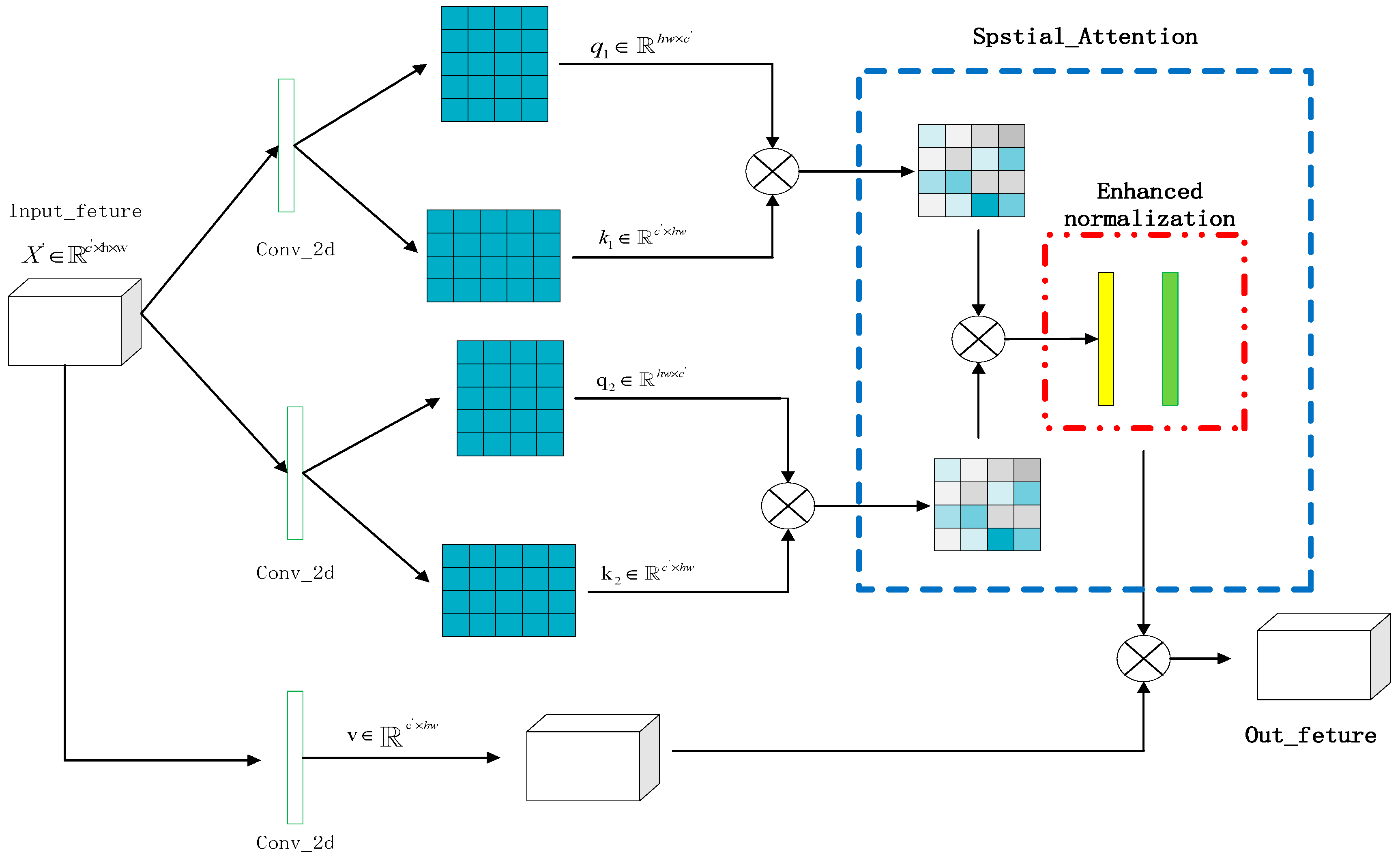
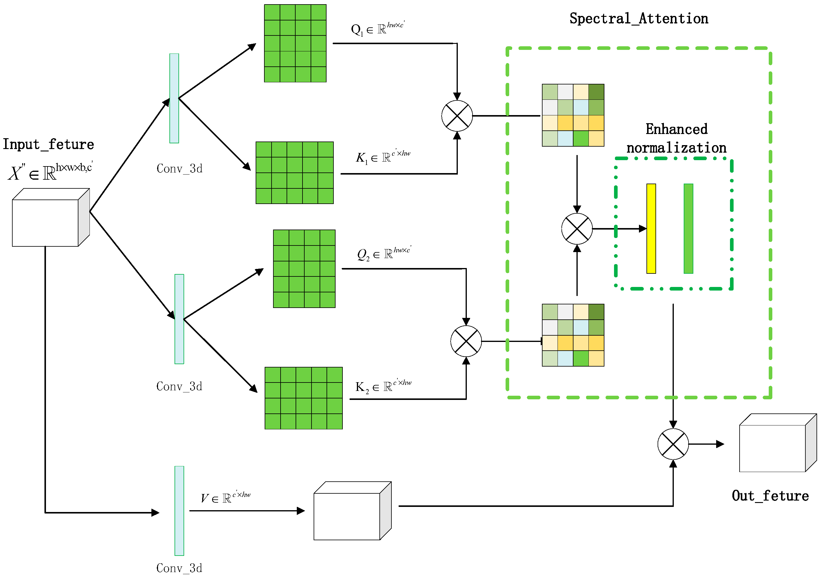
- A DAA module is constructed. The DAA uses dual autocorrelation for attention modeling, which can strengthen the difference between features to enhance the ability to pay attention to important features. In addition, enhanced normalization is proposed to further highlight important features.
- (4)
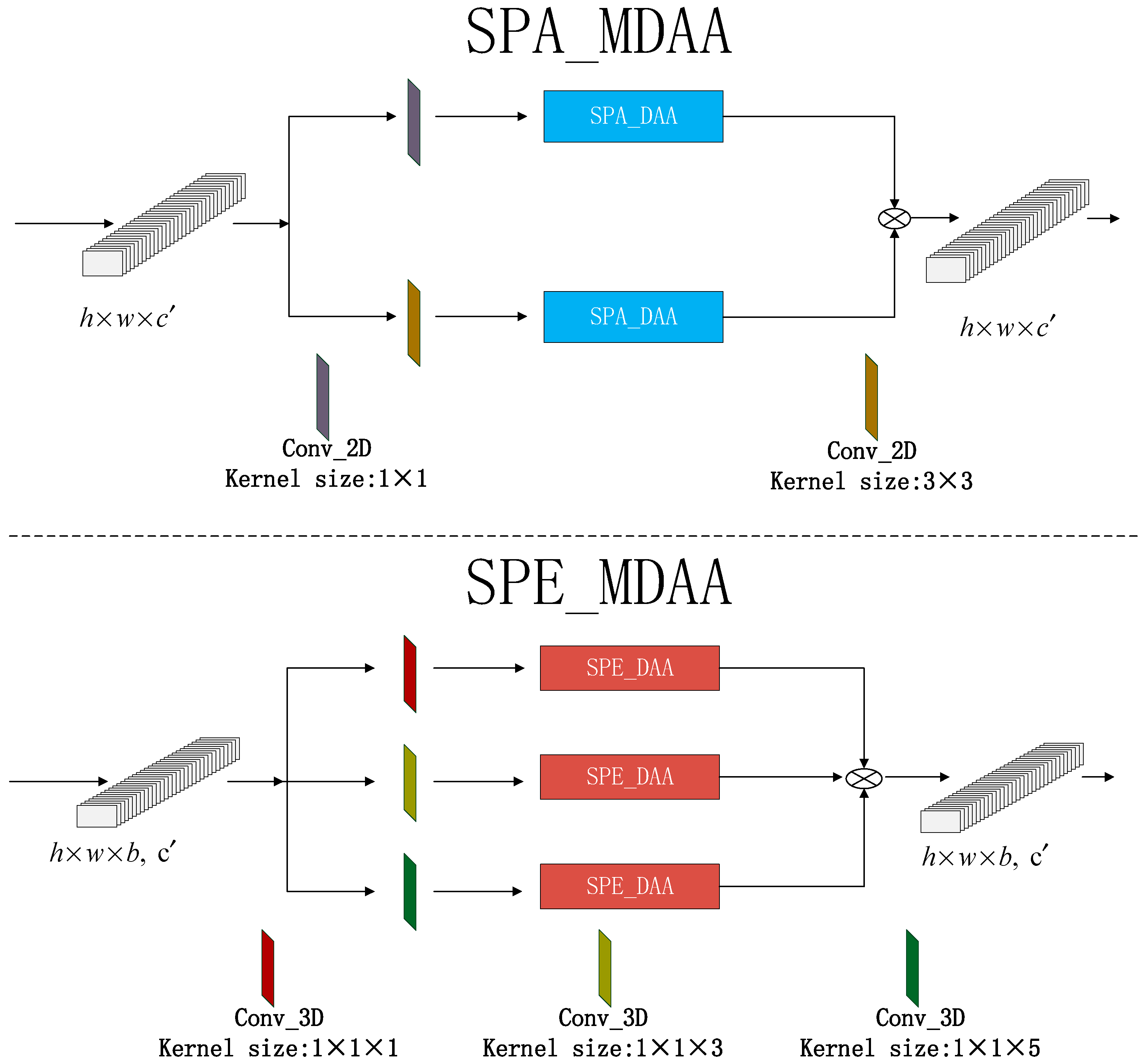
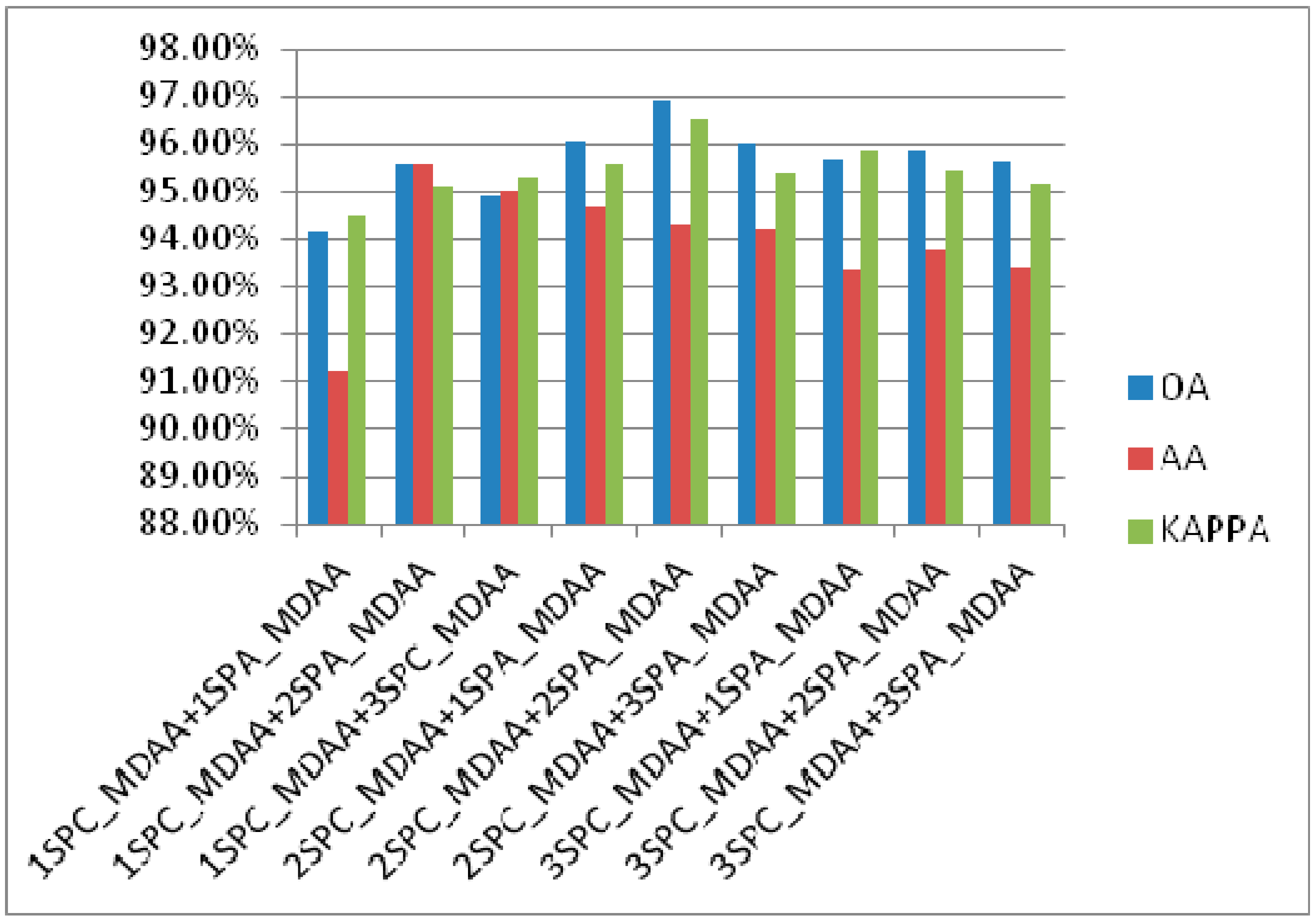
- A multi-scale head strategy is proposed for the DAA mechanism. It can increase the receptive field and obtain the attention value of multiple features to enhance the attention ability.
2. Methods
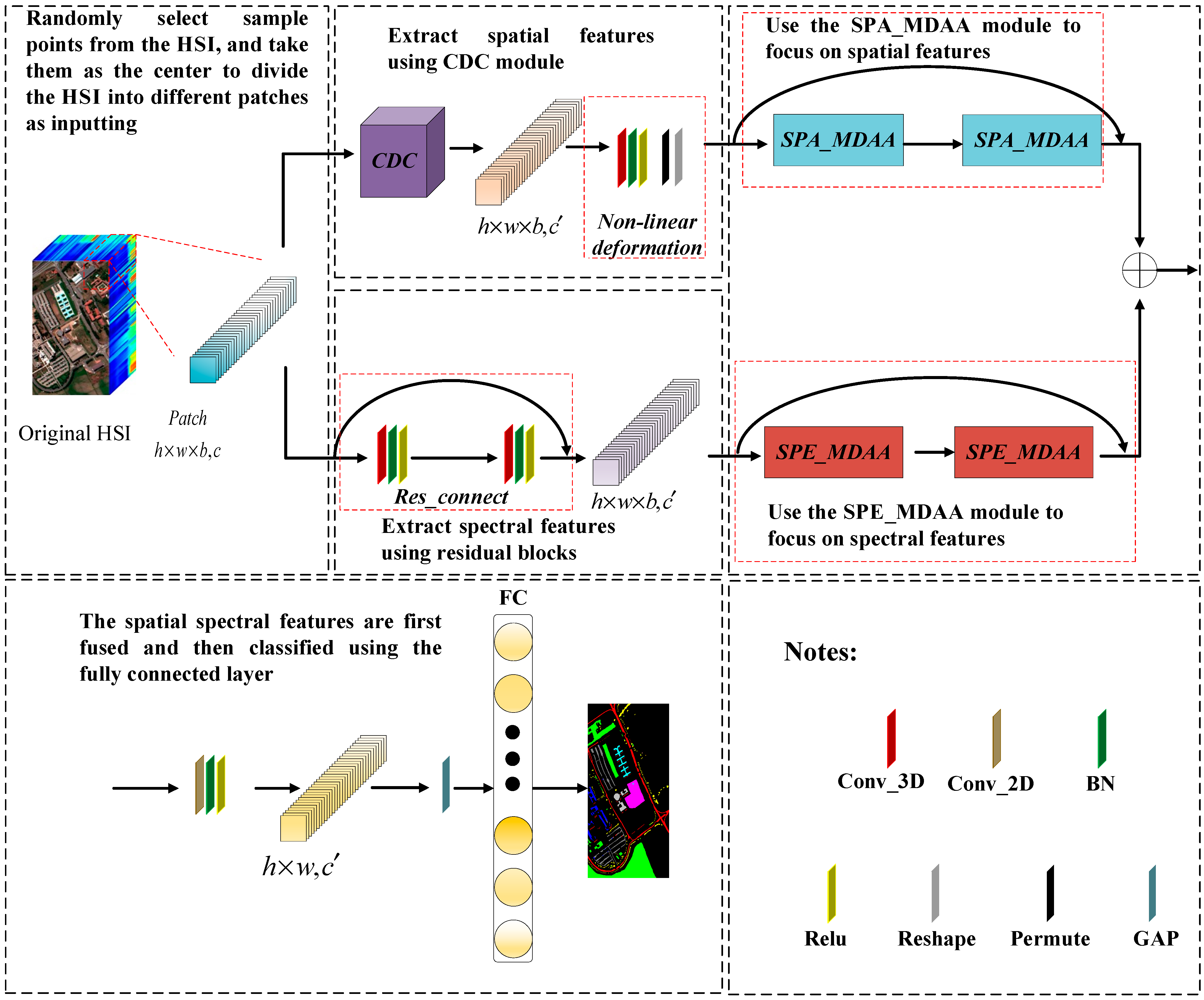
2.1. The Overall Framework of CDC_MDAA
2.2. The CDC Module
| Algorithm 1. The implementation process of the CDC module |
|
2.3. The DAA Module
| Algorithm 2. The detailed implementation process of SPA_DAA module |
|
| Algorithm 3. The implementation process of the SPE_DAA module |
|
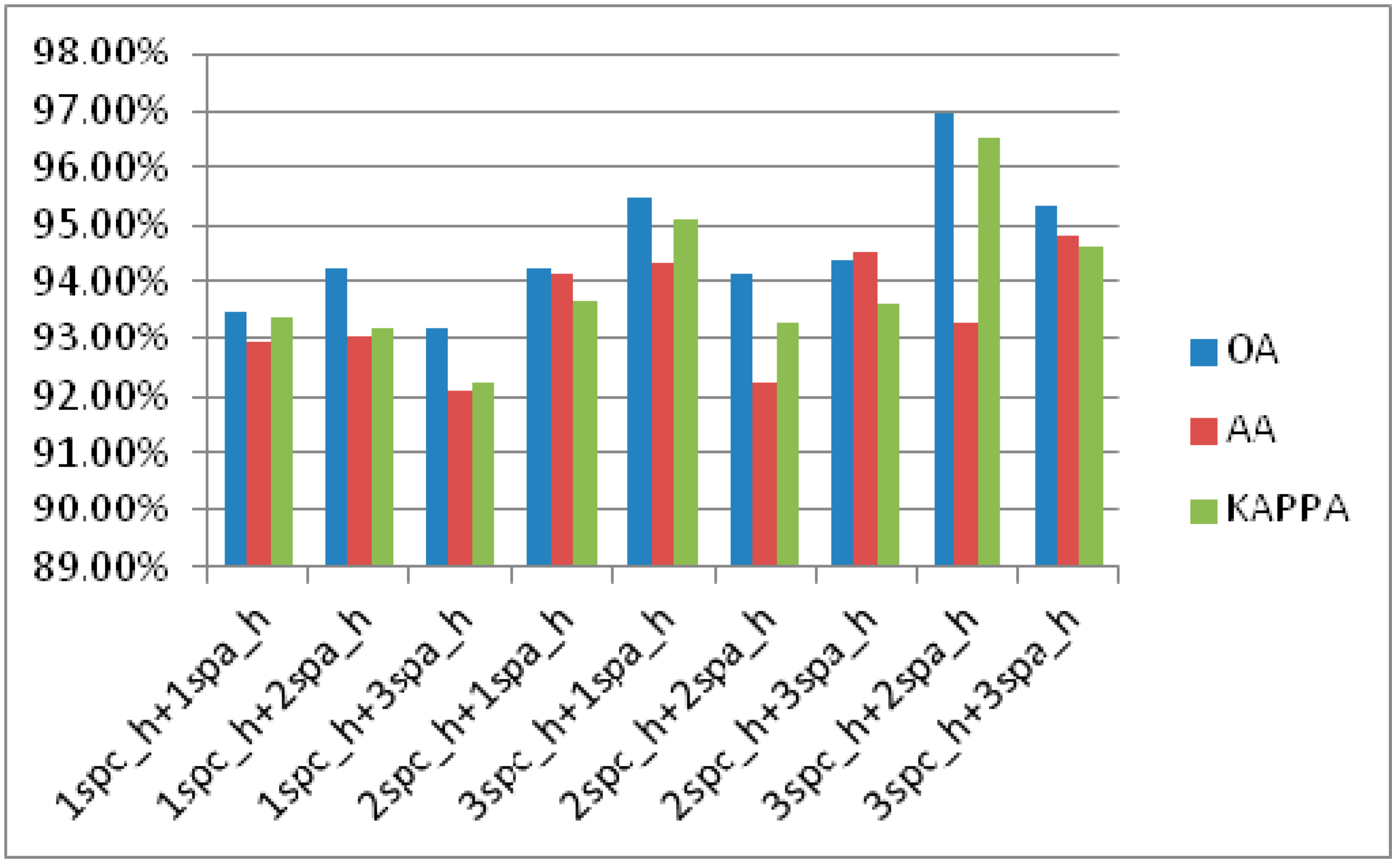
2.4. The Multi-Scale Head Strategy
3. Experimental Results and Analysis
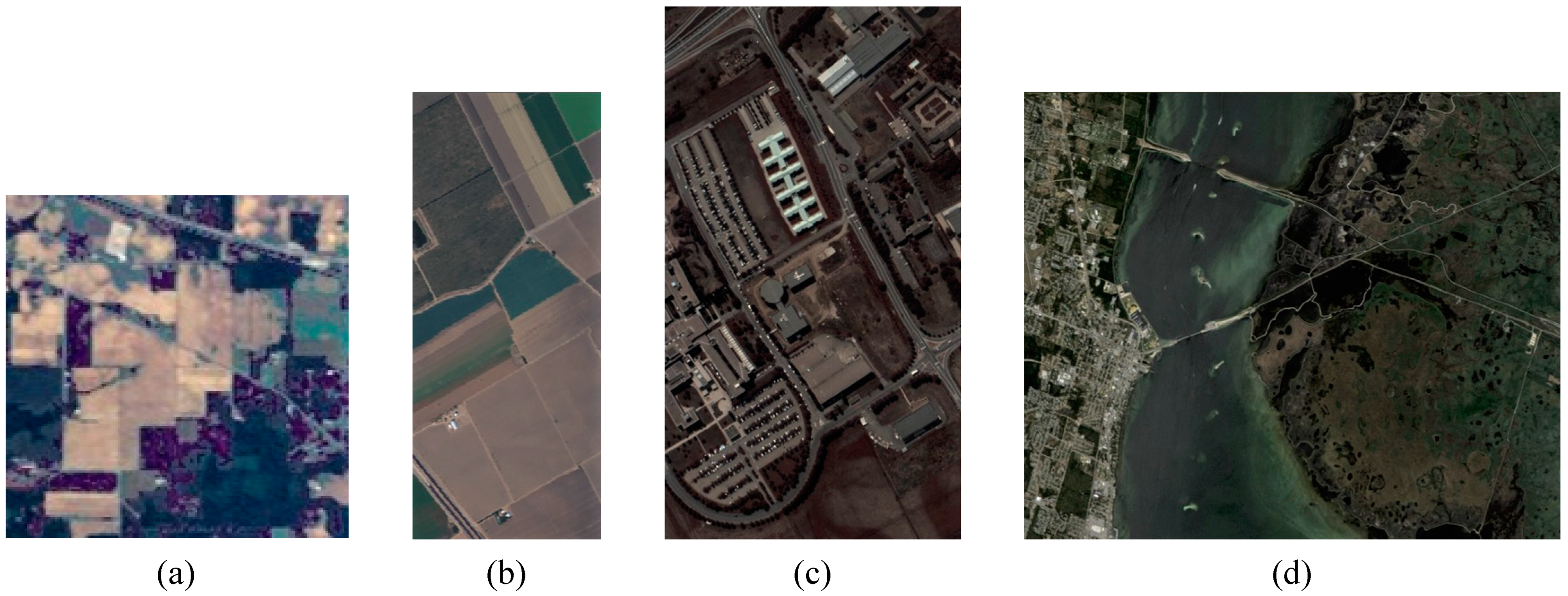
3.1. HSI Datasets
3.2. Experimental Parameters and Model Setting
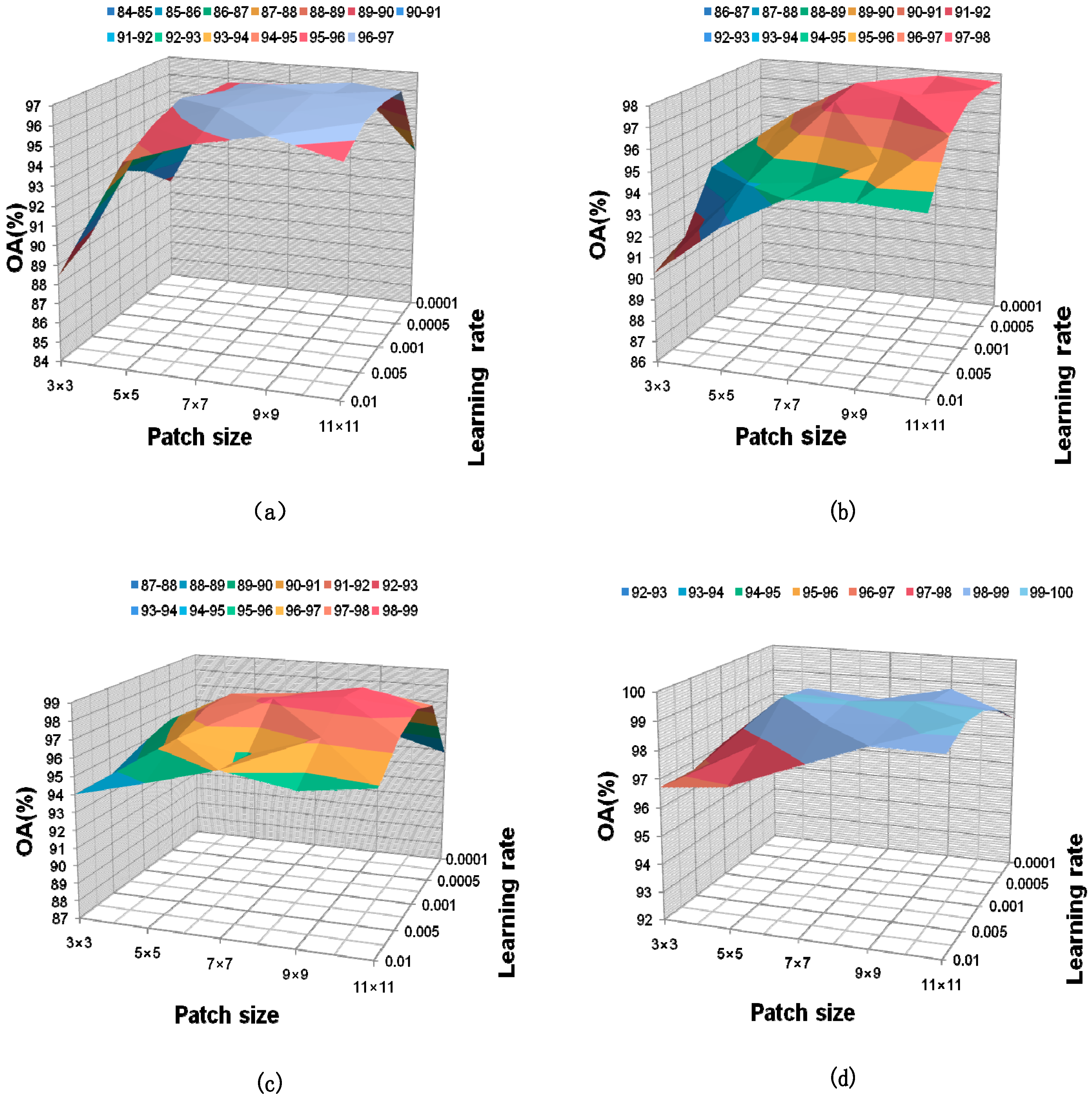
3.2.1. Experimental Parameter Setting
3.2.2. Model Setting
3.3. Experimental Analysis
3.3.1. Effectiveness Analysis of the Proposed Module
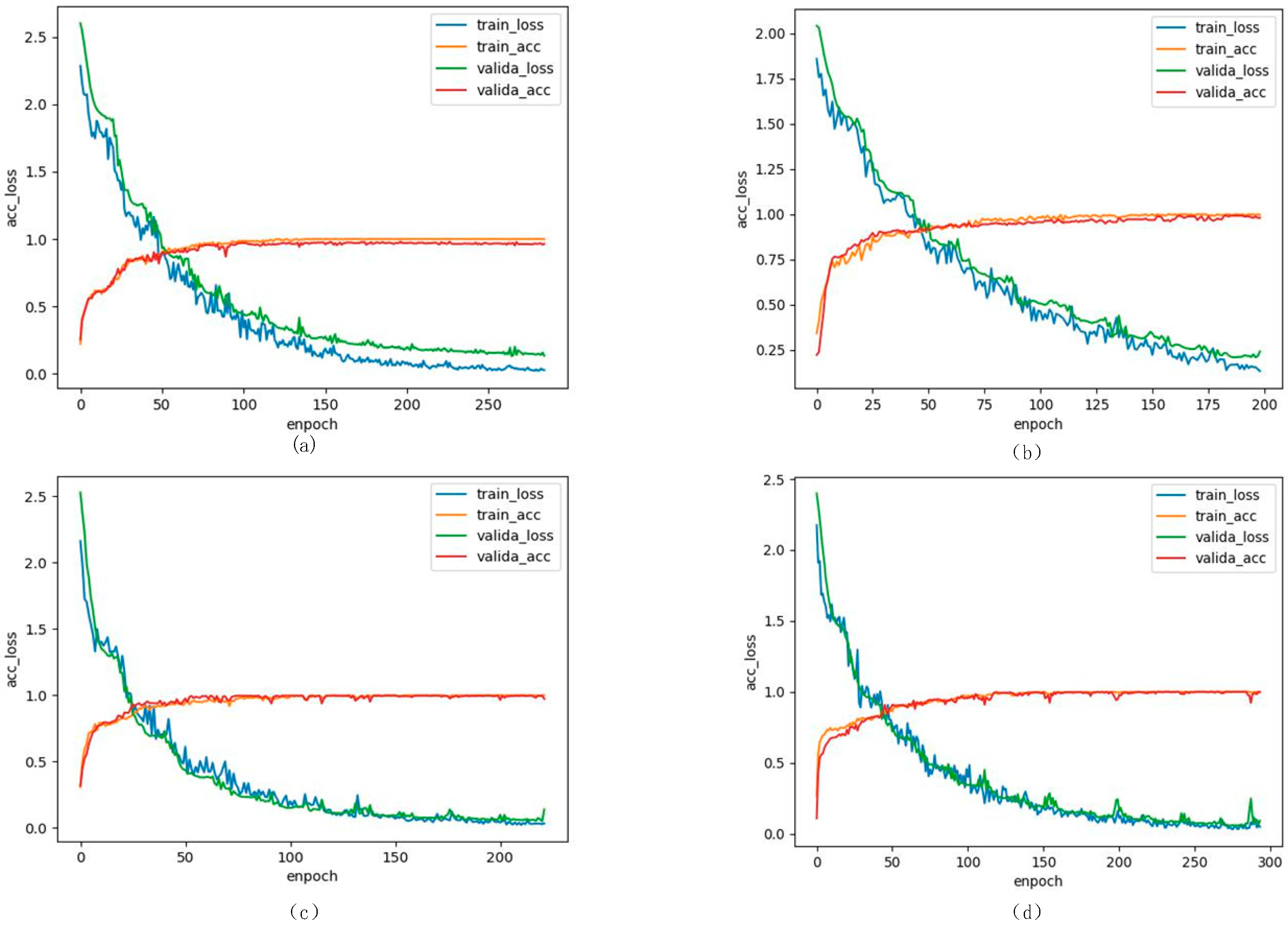
3.3.2. Convergence of Network
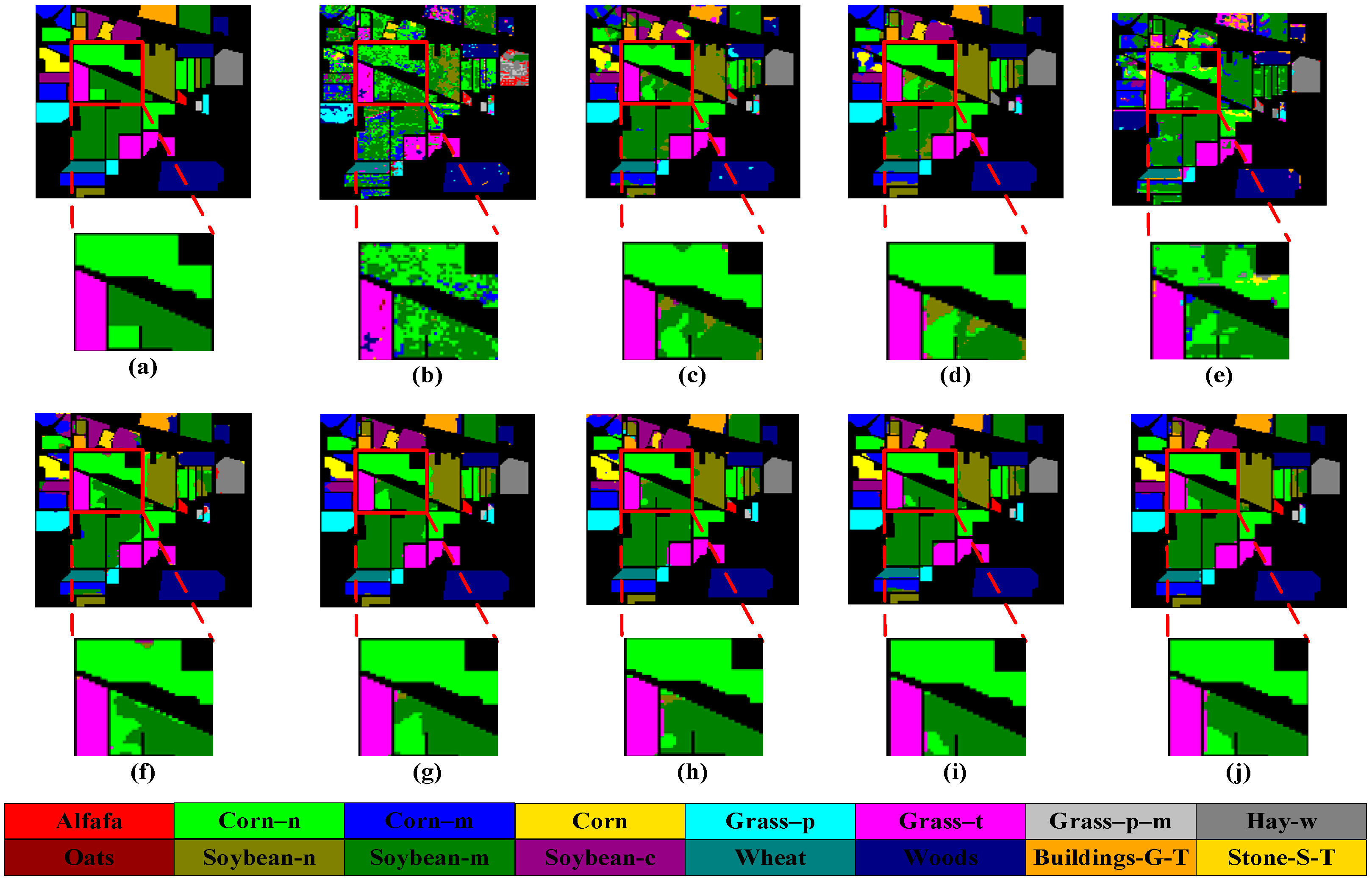
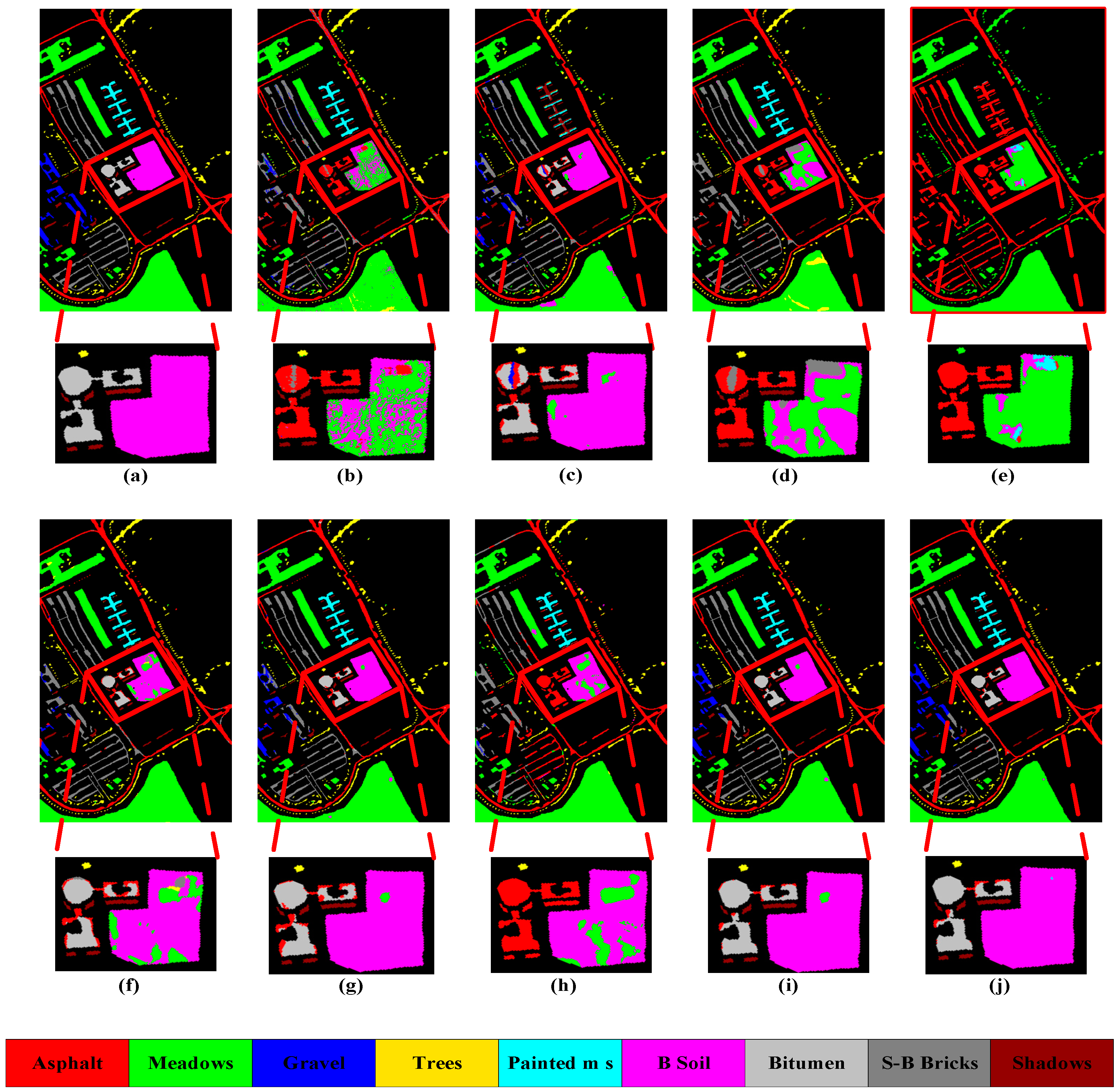
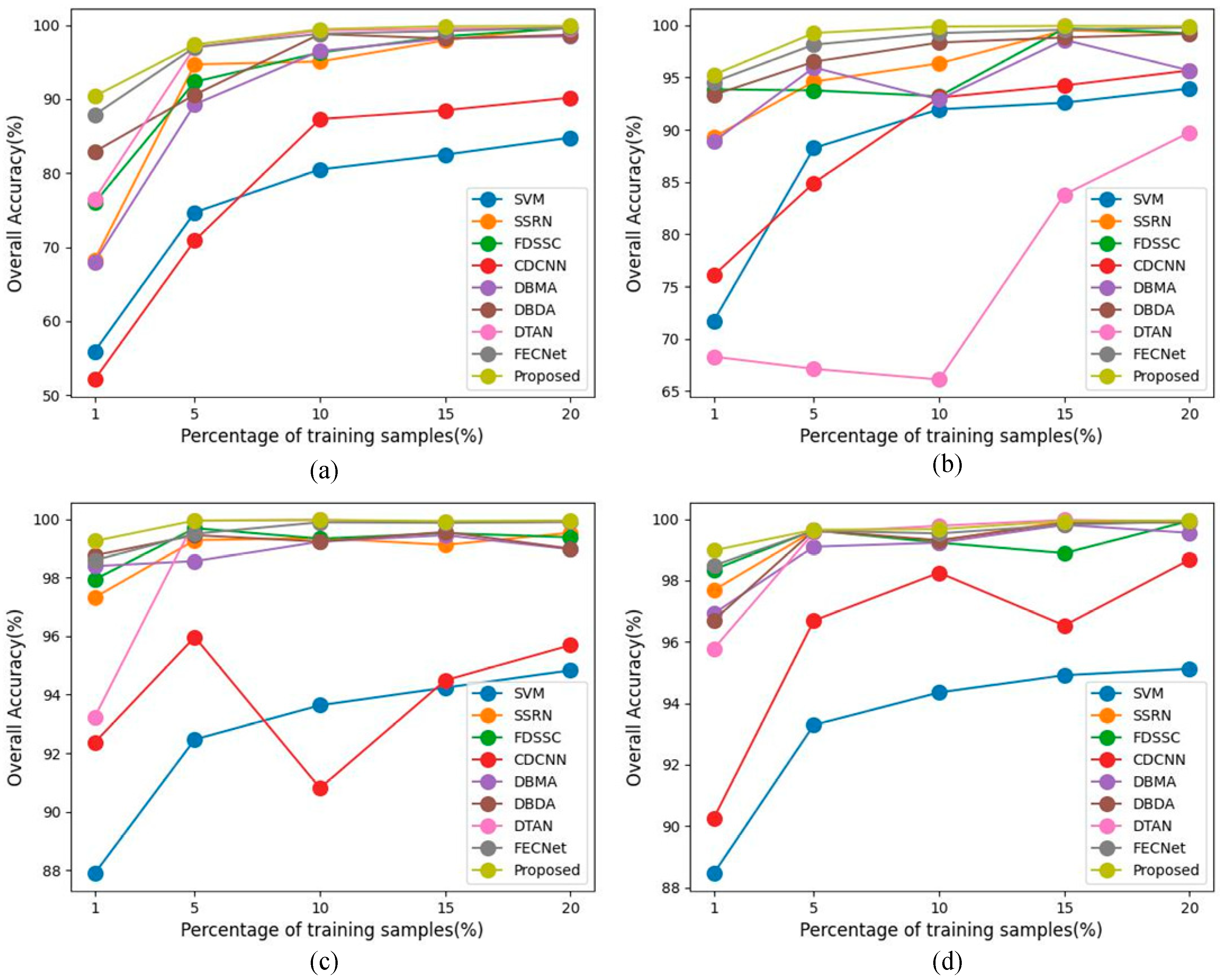
3.3.3. Comparison of Different Methods
4. Conclusions
Author Contributions
Funding
Data Availability Statement
Acknowledgments
Conflicts of Interest
References
- Bioucas-Dias, J.M.; Plaza, A.; Camps-Valls, G.; Scheunders, P.; Nasrabadi, N.; Chanussot, J. Hyperspectral remote sensing data analysis and future challenges. IEEE Geosci. Remote Sens. Mag. 2013, 1, 6–36. [Google Scholar] [CrossRef]
- Landgrebe, D. Hyperspectral image data analysis. IEEE Signal Process. Mag. 2002, 19, 17–28. [Google Scholar] [CrossRef]
- Lacar, F.M.; Lewis, M.M.; Grierson, I.T. “Use of hyperspectral imagery for mapping grape varieties in the Barossa Valley, South Australia”, IGARSS 2001. Scanning the Present and Resolving the Future. In Proceedings of the IEEE 2001 International Geoscience and Remote Sensing Symposium (Cat. No.01CH37217), Sydney, NSW, Australia, 9–13 July 2001; Volume 6, pp. 2875–2877. [Google Scholar]
- Stuffler, T.; Förster, K.; Hofer, S.; Leipold, M.; Sang, B.; Kaufmann, H.; Penné, B.; Mueller, A.; Chlebek, C. Hyperspectral imaging an advanced instrument concept for the Enmap mission (environmental mapping and analysis programme). Acta Astronaut. 2009, 65, 1107–1112. [Google Scholar] [CrossRef]
- Malthus, T.J.; Mumby, P.J. Remote sensing of the coastal zone: An overview and priorities for future research. Int. J. Remote Sens. 2003, 24, 2805–2815. [Google Scholar] [CrossRef]
- Fauvel, M.; Tarabalka, Y.; Benediktsson, J.A.; Chanussot, J.; Tilton, J.C. Advances in spectral-spatial classification of hyperspectral images. Proc. IEEE 2013, 101, 652–675. [Google Scholar] [CrossRef]
- Samaniego, L.; Bardossy, A.; Schulz, K. Supervised classification of remotely sensed imagery using a modified k-NN technique. IEEE Trans. Geosci. Remote Sens. 2008, 46, 2112–2125. [Google Scholar] [CrossRef]
- Ediriwickrema, J.; Khorram, S. Hierarchical maximum-likelihood classification for improved accuracies. IEEE Trans. Geosci. Remote Sens. 1997, 35, 810–816. [Google Scholar] [CrossRef]
- Foody, G.M.; Mathur, A. A relative evaluation of multi-class image classification by support vector machines. IEEE Trans. Geosci. Remote Sens. 2004, 42, 1335–1343. [Google Scholar] [CrossRef]
- Prasad, S.; Bruce, L.M. Limitations of princinal components analysis for hyperspectral target recognition. IEEE Geosci. Remote Sens. Lett. 2008, 5, 625–629. [Google Scholar] [CrossRef]
- Benediktsson, J.A.; Chanussot, J.; Moon, W.M. Very high-resolution remote sensing: Challenges and opportunities [point of view]. Proc. IEEE 2012, 100, 1907–1910. [Google Scholar] [CrossRef]
- Chen, Y.S.; Zhao, X.; Jia, X.P. Spectral-spatial classification of hyperspectral data based on deep belief network. IEEE J. Sel. Top. Appl. Earth Obs. Remote Sens. 2015, 8, 2381–2392. [Google Scholar] [CrossRef]
- Sun, L.; Wu, Z.B.; Liu, J.J.; Xiao, L.; Wei, Z.H. Supervised spectral-spatial hyperspectral image classification with weighted Markov random fields. IEEE Trans. Geosci. Remote Sens. 2015, 53, 1490–1503. [Google Scholar] [CrossRef]
- Chen, Y.S.; Lin, Z.H.; Zhao, X.; Wang, G.; Gu, Y.F. Deep learning based classification of hyperspectral data. IEEE J. Sel. Top. IN Appl. Earth Obs. Remote Sens. 2014, 7, 2094–2107. [Google Scholar] [CrossRef]
- Yuan, Y.; Meng, X.; Sun, W.; Yang, G.; Wang, L.; Peng, J.; Wang, Y. Multi-Resolution Collaborative Fusion of SAR, Multispectral and Hyperspectral Images for Coastal Wetlands Mapping. Remote Sens. 2022, 14, 3492. [Google Scholar] [CrossRef]
- Sun, W.; Kai Liu Ren, G.; Liu, W.; Yang, G.; Meng, X.; Peng, J. A simple and effective spectral-spatial method for mapping large-scale coastal wetlands using China ZY1-02D satellite hyperspectral images. Int. J. Appl. Earth Obs. Geoinf. 2021, 104, 102572. [Google Scholar] [CrossRef]
- Yang, J.; Zhang, D.; Frangi, A.F.; Yang, J.Y. Two-dimensional PCA: A new approach to appearance-based face representation and recognition. IEEE Trans. Pattern Anal. Mach. Intell. 2004, 26, 131–137. [Google Scholar] [CrossRef]
- Li, W.; Wu, G.; Zhang, F.; Du, Q. Hyperspectral image classification using deep pixel-pair features. IEEE Trans. Geosci. Remote Sens. 2017, 55, 844–853. [Google Scholar] [CrossRef]
- Makantasis, K.; Karantzalos, K.; Doulamis, A.; Doulamis, N. Deep supervised learning for hyperspectral data classification through convolutional neural networks. In Proceedings of the 2015 IEEE International Geoscience and Remote Sensing Symposium (IGARSS), Milan, Italy, 26–31 July 2015; pp. 4959–4962. [Google Scholar]
- Shao, W.; Du, S. Spectral-spatial feature extraction for hyperspectral image classification: A dimension reduction and deep learning approach. IEEE Trans. Geosci. Remote Sens. 2016, 54, 4544–4554. [Google Scholar]
- Mei, S.; Ji, J.; Hou, J.; Li, X.; Du, Q. Learning sensor-specific spatial-spectral features of hyperspectral images via convolutional neural networks. IEEE Trans. Geosci. Remote Sens. 2017, 55, 4520–4533. [Google Scholar] [CrossRef]
- Yue, J.; Zhao, W.; Mao, S.; Liu, H. Spectral-spatial classification of hyperspectral images using deep convolutional neural networks. Remote Sens. Lett. 2015, 6, 468–477. [Google Scholar] [CrossRef]
- Lecun, Y.; Bengio, Y.; Hinton, G. Deep learning. Nature 2015, 521, 436. [Google Scholar] [CrossRef]
- Ghamisi, P.; Maggiori, E.; Li, S.; Souza, R.; Tarablaka, Y.; Moser, G.; De Giorgi, A.; Fang, L.; Chen, Y.; Chi, M.; et al. New frontiers IN spectral-spatial hyperspectral image classification: The latest advances based on mathematical morphology, Markov random fields, segmentation, sparse representation, and deep learning. IEEE Geosci. Remote Sens. Mag. 2018, 6, 10–43. [Google Scholar] [CrossRef]
- Chen, Y.; Jiang, H.; Li, C.; Jia, X.; Ghamisi, P. Deep feature extraction and classification of hyperspectral images based on convolutional neural networks. IEEE Trans. Geosci. Remote Sens. 2016, 54, 6232–6251. [Google Scholar] [CrossRef]
- He, K.; Zhang, X.; Ren, S.; Sun, J. Deep residual learning for image recognition. In Proceedings of the IEEE Conference on Computer Vision and Pattern Recognition, Las Vegas, NV, USA, 27–30 June 2016; pp. 770–778. [Google Scholar]
- Paoletti, M.E.; Haut, J.M.; Plaza, J.; Plaza, A. Deep&dense convolutional neural network for hyperspectral image classification. Remote Sens. 2018, 10, 1454. [Google Scholar]
- Yu, C.; Han, R.; Song, M.; Liu, C.; Chang, C.-I. Feedback Attention-Based Dense CNN for Hyperspectral Image Classification. IEEE Trans. Geosci. Remote Sens. 2022, 60, 5501916. [Google Scholar] [CrossRef]
- Zhao, C.; Qin, B.; Li, T.; Feng, S.; Yan, Y. Hyperspectral Image Classification Based on Dense Convolution and Conditional Random Field. In Proceedings of the 2021 IEEE International Geoscience and Remote Sensing Symposium IGARSS, Brussels, Belgium, 11–16 July 2021; pp. 3653–3656. [Google Scholar]
- Zhang, H.; Yu, H.; Xu, Z.; Zheng, K.; Gao, L. A Novel Classification Framework for Hyperspectral Image Classification Based on Multi-Scale Dense Network. In Proceedings of the 2021 IEEE International Geoscience and Remote Sensing Symposium IGARSS, Brussels, Belgium, 11–16 July 2021; pp. 2238–2241. [Google Scholar]
- Yang, G.; Gewali, U.B.; Ientilucci, E.; Gartley, M.; Monteiro, S.T. Dual-Channel Densenet for Hyperspectral Image Classification. In Proceedings of the IGARSS 2018—2018 IEEE International Geoscience and Remote Sensing Symposium, Valencia, Spain, 22–27 July 2018; pp. 2595–2598. [Google Scholar]
- Paoletti, M.E.; Haut, J.M.; Fernandez-Beltran, R.; Plaza, J.; Plaza, A.J.; Pla, F. Deep Pyramidal Residual Networks for Spectral–Spatial Hyperspectral Image Classification. IEEE Trans. Geosci. Remote Sens. 2019, 57, 740–754. [Google Scholar] [CrossRef]
- Pande, S.; Banerjee, B. Dimensionality Reduction Using 3D Residual Autoencoder for Hyperspectral Image Classification. In Proceedings of the IGARSS 2020—2020 IEEE International Geoscience and Remote Sensing Symposium, Waikoloa, HI, USA, 19–24 July 2020; pp. 2029–2032. [Google Scholar]
- Zhang, C.; Li, G.; Du, S. Multi-Scale Dense Networks for Hyperspectral Remote Sensing Image Classification. IEEE Trans. Geosci. Remote Sens. 2019, 57, 9201–9222. [Google Scholar] [CrossRef]
- Li, Z.; Wang, T.; Li, W.; Du, Q.; Wang, C.; Liu, C.; Shi, X. Deep Multilayer Fusion Dense Network for Hyperspectral Image Classification. IEEE J. Sel. Top. Appl. Earth Obs. Remote Sens. 2020, 13, 1258–1270. [Google Scholar] [CrossRef]
- Wang, X.; Tan, K.; Du, P.; Pan, C.; Ding, J. A Unified Multiscale Learning Framework for Hyperspectral Image Classification. IEEE Trans. Geosci. Remote Sens. 2022, 60, 4508319. [Google Scholar] [CrossRef]
- Haut, Z.M.; Paoletti, M.E.; Plaza, J.; Plaza, A.; Li, J. Visual attention-driven hyperspectral image classification. IEEE Trans. Geosci. Remote Sens. 2019, 57, 8065–8080. [Google Scholar] [CrossRef]
- Woo, S.; Park, J.; Lee, J.; Kweon, I. Cbam: Convolutional block attention module. In Proceedings of the European Conference on Computer Vision (ECCV), Amsterdam, The Netherlands, 8–16 October 2018; pp. 3–19. [Google Scholar]
- Sun, H.; Zheng, X.; Lu, X.; Wu, S. Spectral–spatial attention network for hyperspectral image classification. IEEE Trans. Geosci. Remote Sens. 2020, 58, 3232–3245. [Google Scholar] [CrossRef]
- Mei, X.; Pan, E.; Ma, Y.; Dai, X.; Huang, J.; Fan, F.; Du, Q.; Zheng, H.; Ma, J. Spectral–spatial attention networks for hyperspectral image classification. Remote Sens. 2019, 11, 963. [Google Scholar] [CrossRef]
- Hang, R.; Li, Z.; Liu, Q.; Ghamisi, P.; Bhattacharyya, S.S. Hyperspectral Image Classification with Attention-Aided CNNs. IEEE Trans. Geosci. Remote Sens. 2021, 59, 2281–2293. [Google Scholar] [CrossRef]
- Zheng, X.; Sun, H.; Lu, X.; Xie, W. Rotation-Invariant Attention Network for Hyperspectral Image Classification. IEEE Trans. Image Process. 2022, 31, 4251–4265. [Google Scholar] [CrossRef] [PubMed]
- Yang, K.; Sun, H.; Zou, C.; Lu, X. Cross-Attention Spectral–Spatial Network for Hyperspectral Image Classification. IEEE Trans. Geosci. Remote Sens. 2022, 60, 5518714. [Google Scholar] [CrossRef]
- Ma, W.; Yang, Q.; Wu, Y.; Zhao, W.; Zhang, X. Double-Branch Multi-Attention Mechanism Network for Hyperspectral Image Classification. Remote Sens. 2019, 11, 1307. [Google Scholar] [CrossRef]
- Fu, J.; Liu, J.; Tian, H.; Li, Y.; Bao, Y.; Fang, Z.; Lu, H. Dual attention network for scene segmentation. In Proceedings of the IEEE/CVF Conference on Computer Vision and Pattern Recognition, Long Beach, CA, USA, 15–20 June 2019; pp. 3146–3154. [Google Scholar]
- Liu, K.; Sun, W.; Shao, Y.; Liu, W.; Yang, G.; Meng, X.; Peng, J.; Mao, D.; Ren, K. Mapping Coastal Wetlands Using Transformer in Transformer Deep Network on China ZY1-02D Hyperspectral Satellite Images. IEEE J. Sel. Top. Appl. Earth Obs. Remote Sens. 2022, 15, 3891–3903. [Google Scholar] [CrossRef]
- Melgani, F.; Bruzzone, L. Classification of hyperspectral remote sensing images with support vector machines. IEEE Trans. Geosci. Remote Sens. 2004, 42, 1778–1790. [Google Scholar] [CrossRef]
- Lee, H.; Kwon, H. Going Deeper with Contextual CNN for Hyperspectral Image Classification. IEEE Trans. Image Process. 2017, 26, 4843–4855. [Google Scholar] [CrossRef]
- Wang, W.; Dou, S.; Jiang, Z.; Sun, L. A Fast Dense Spectral–Spatial Convolution Network Framework for Hyperspectral Images Classification. Remote Sens. 2018, 10, 1068. [Google Scholar] [CrossRef]
- Zhong, Z.; Li, J.; Luo, Z.; Chapman, M. Spectral–Spatial Residual Network for Hyperspectral Image Classification: A 3-D DeepLearning Framework. IEEE Trans. Geosci. Remote Sens. 2017, 56, 847–858. [Google Scholar] [CrossRef]
- Cui, Y.; Yu, Z.; Han, J.; Gao, S.; Wang, L. Dual-Trinle Attention Network for Hyperspectral Image Classification Using Limited Training Samples. IEEE Geosci. Remote Sens. Lett. 2022, 19, 5504705. [Google Scholar] [CrossRef]
- Shi, C.; Liao, D.; Zhang, T.; Wang, L. Hyperspectral Image Classification Based on Expansion Convolution Network. IEEE Trans. Geosci. Remote Sens. 2022, 60, 5528316. [Google Scholar] [CrossRef]
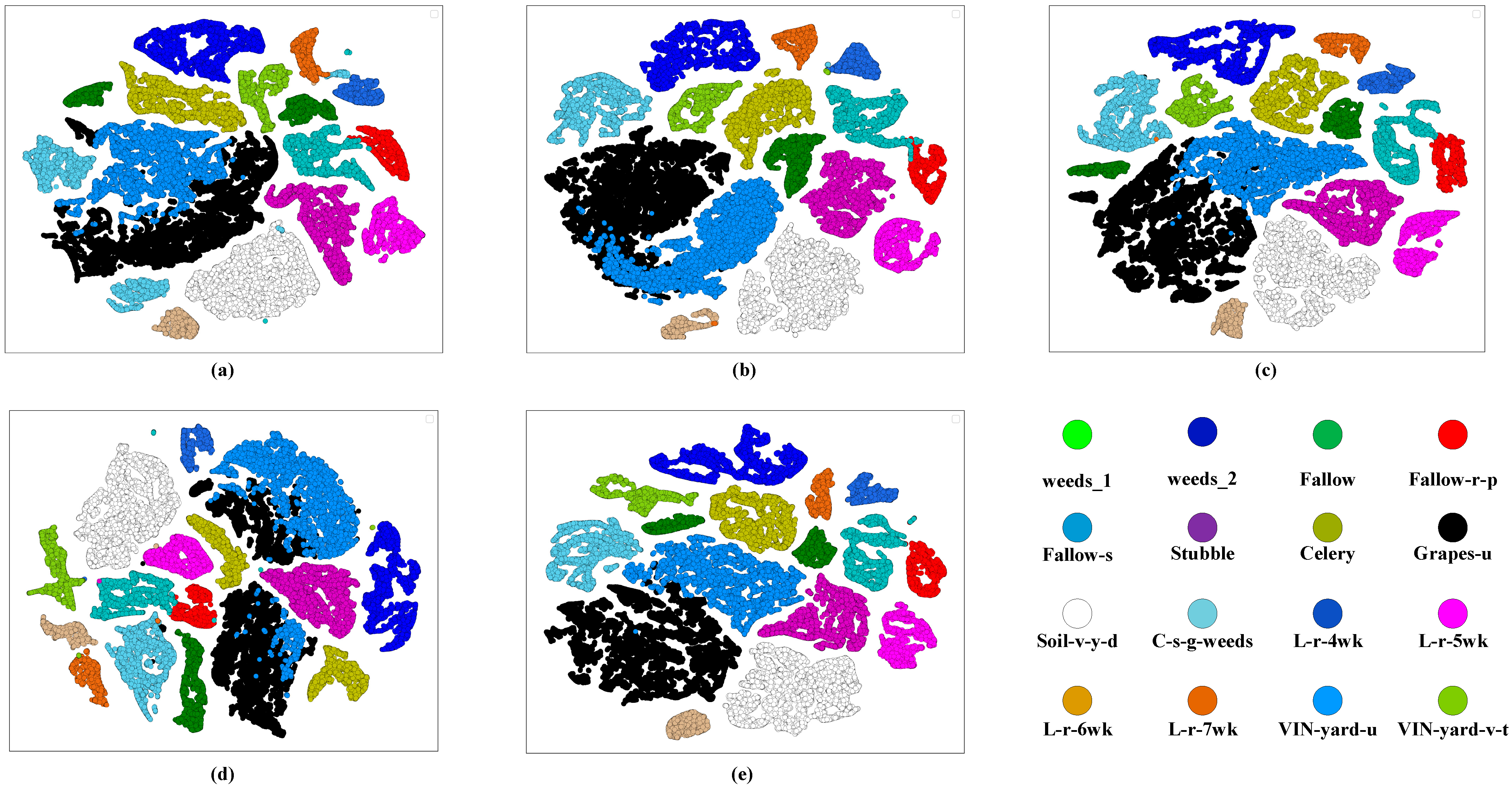
- Van der Maaten, L.; Hinton, G. Visualizing data using t-SNE. J. Mach. Learn. Res. 2008, 9, 2579–2605. [Google Scholar]


 Ground truth | NO. | Lengend | Name | Sample |
| 1 |  | Alfafa | 46 | |
| 2 |  | Corn–n | 1428 | |
| 3 |  | Corn–m | 830 | |
| 4 |  | Corn | 237 | |
| 5 |  | Grass–p | 483 | |
| 6 |  | Grass–t | 730 | |
| 7 |  | Grass–p–m | 28 | |
| 8 |  | Hay-w | 478 | |
| 9 |  | Oats | 20 | |
| 10 |  | Soybean-n | 972 | |
| 11 |  | Soybean-m | 2455 | |
| 12 |  | Soybean-c | 593 | |
| 13 |  | Wheat | 205 | |
| 14 |  | Woods | 1265 | |
| 15 |  | Buildings-G-T | 386 | |
| 16 |  | Stone-S-T | 93 |
 Ground truth | NO. | Lengend | Name | Sample |
| 1 |  | Asphalt | 6631 | |
| 2 |  | Meadows | 18,649 | |
| 3 |  | Gravel | 2099 | |
| 4 |  | Trees | 3064 | |
| 5 |  | Painted m s | 1345 | |
| 6 |  | B Soil | 5029 | |
| 7 |  | Bitumen | 1330 | |
| 8 |  | S-B Bricks | 3682 | |
| 9 |  | Shadows | 947 |
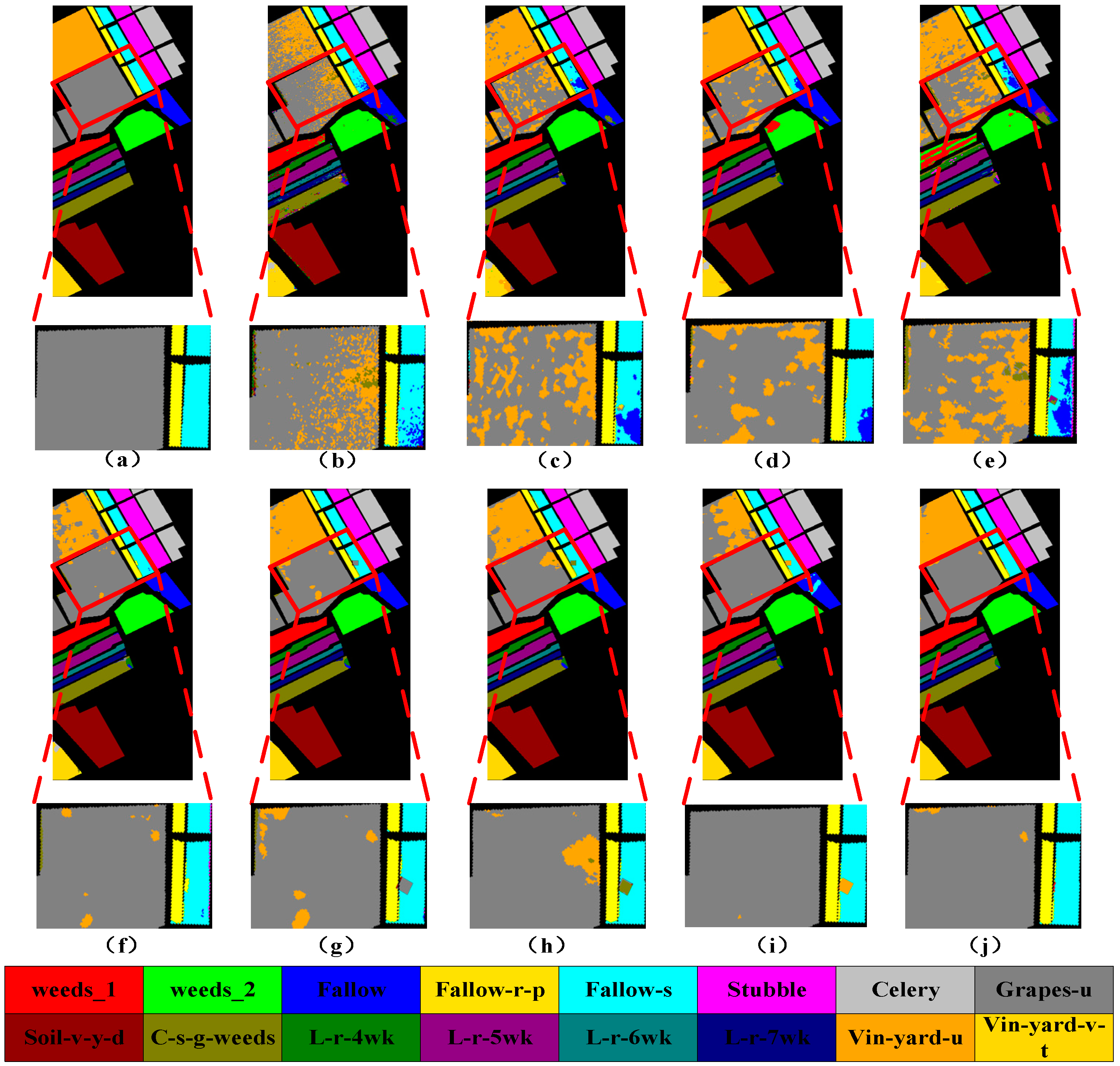
 Ground truth | NO. | Lengend | Name | Sample |
| 1 |  | weeds_1 | 2009 | |
| 2 |  | weeds_2 | 3726 | |
| 3 |  | Fallow | 1976 | |
| 4 |  | Fallow-r-p | 1394 | |
| 5 |  | Fallow-s | 2678 | |
| 6 |  | Stubble | 3959 | |
| 7 |  | Celery | 3579 | |
| 8 |  | Grapes-u | 11,271 | |
| 9 |  | Soil-v-y-d | 6203 | |
| 10 |  | C-s-g-weeds | 3278 | |
| 11 |  | L-r-4wk | 1068 | |
| 12 |  | L-r-5wk | 1927 | |
| 13 |  | L-r-6wk | 916 | |
| 14 |  | L-r-7wk | 1070 | |
| 15 |  | VIN-yard-u | 7268 | |
| 16 |  | VIN-yard-v-t | 1807 |
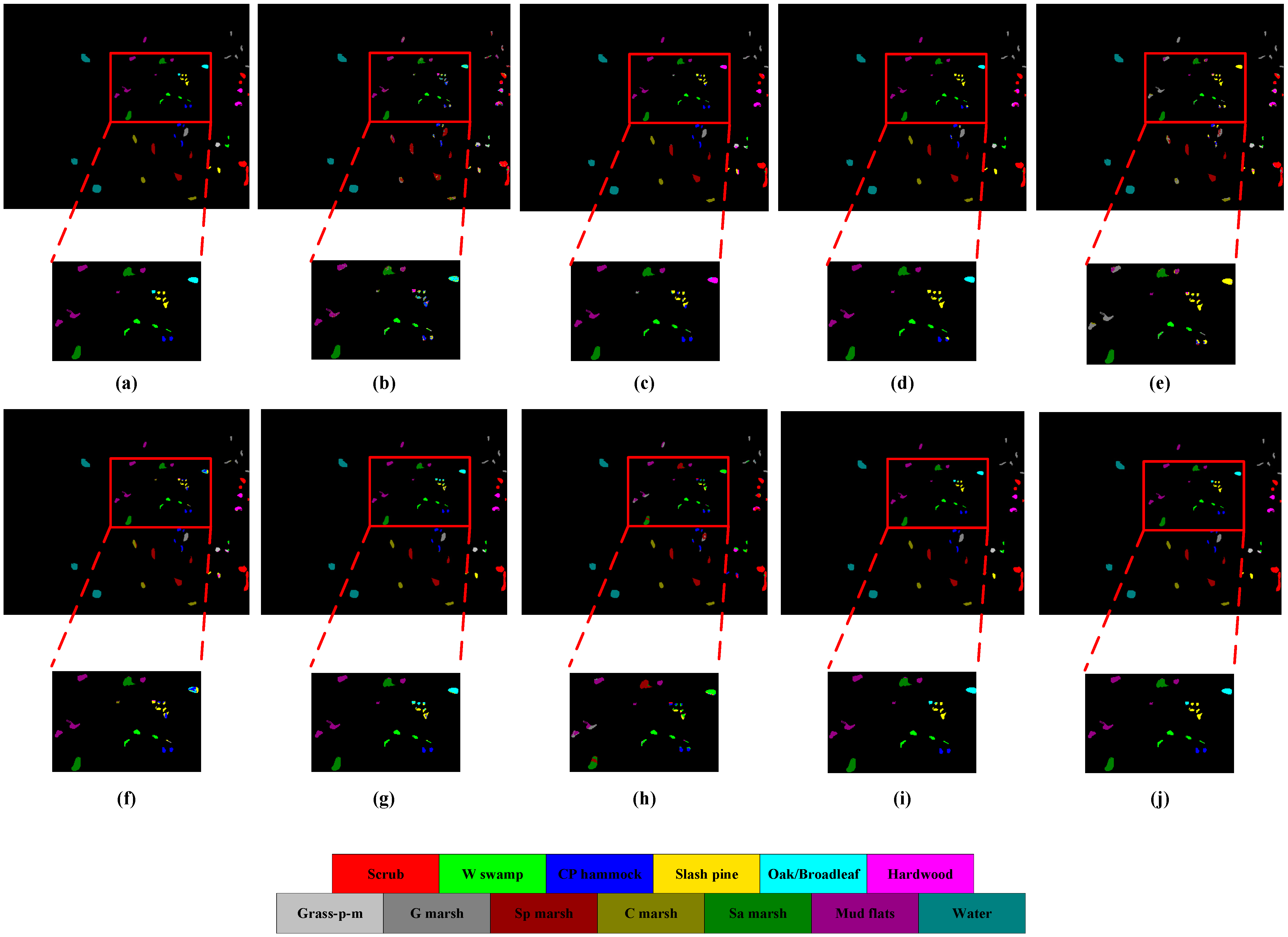
 Ground truth | NO. | Lengend | Name | Sample |
| 1 |  | Scrub | 761 | |
| 2 |  | W swamp | 243 | |
| 3 |  | CP hammock | 256 | |
| 4 |  | Slash pine | 252 | |
| 5 |  | Oak/Broadleaf | 161 | |
| 6 |  | Hardwood | 229 | |
| 7 |  | Grass-p-m | 105 | |
| 8 |  | G marsh | 431 | |
| 9 |  | Sp marsh | 520 | |
| 10 |  | C marsh | 404 | |
| 11 |  | Sa marsh | 419 | |
| 12 |  | Mud flats | 503 | |
| 13 |  | Water | 927 |
| STRATEGY | OA | AA | KAPPA |
|---|---|---|---|
| Without CDC | 92.71% | 94.02% | 91.74% |
| With CDC | 96.94% | 94.31% | 96.51% |
| STRATEGY | OA | AA | KAPPA |
|---|---|---|---|
| Without SPA_MDAA | 88.76% | 85.24% | 85.83% |
| With SPA_MDAA | 96.94% | 94.31% | 96.51% |
| STRATEGY | OA | AA | KAPPA |
|---|---|---|---|
| Without SPE_MDAA | 91.45% | 92.31% | 92.55% |
| With SPE_MDAA | 96.94% | 94.31% | 96.51% |
| Class | SVM | SSRN | FDSSC | CDCNN | DBMA | DBDA | DTAN | FECNet | Proposed |
|---|---|---|---|---|---|---|---|---|---|
| 1 | 36.62 | 81.03 | 85.72 | 24.67 | 77.33 | 99.06 | 30.00 | 99.06 | 100.0 |
| 2 | 55.48 | 87.48 | 93.35 | 49.93 | 78.68 | 92.74 | 93.87 | 96.63 | 98.84 |
| 3 | 62.33 | 76.35 | 89.51 | 31.93 | 76.12 | 92.28 | 95.12 | 93.25 | 98.69 |
| 4 | 42.53 | 73.88 | 93.68 | 33.52 | 75.11 | 94.46 | 94.55 | 95.61 | 95.41 |
| 5 | 85.05 | 84.28 | 92.61 | 71.47 | 94.91 | 99.10 | 94.63 | 98.55 | 100.0 |
| 6 | 83.31 | 92.68 | 98.31 | 73.42 | 93.99 | 98.28 | 99.21 | 97.51 | 96.89 |
| 7 | 59.86 | 79.06 | 82.46 | 36.29 | 44.33 | 66.57 | 50.00 | 73.14 | 62.50 |
| 8 | 89.67 | 96.85 | 97.54 | 78.08 | 97.49 | 99.24 | 92.73 | 99.84 | 100.0 |
| 9 | 39.27 | 73.57 | 71.07 | 42.14 | 45.66 | 93.64 | 20.00 | 79.71 | 84.21 |
| 10 | 62.31 | 84.45 | 89.30 | 41.71 | 77.27 | 93.77 | 92.50 | 90.09 | 89.49 |
| 11 | 64.72 | 86.95 | 93.97 | 55.67 | 83.89 | 93.83 | 93.55 | 96.11 | 98.97 |
| 12 | 50.54 | 83.31 | 88.25 | 27.68 | 77.65 | 90.65 | 89.12 | 93.20 | 95.85 |
| 13 | 86.73 | 98.83 | 99.53 | 67.88 | 96.74 | 97.48 | 99.89 | 98.34 | 100.0 |
| 14 | 88.67 | 95.13 | 95.82 | 76.39 | 93.41 | 97.69 | 95.31 | 97.28 | 95.87 |
| 15 | 61.81 | 88.58 | 92.48 | 47.30 | 76.83 | 93.79 | 93.54 | 95.11 | 96.75 |
| 16 | 98.66 | 96.52 | 98.22 | 65.67 | 92.33 | 93.67 | 93.21 | 97.26 | 95.45 |
| OA(%) | 68.76 | 86.68 | 92.37 | 59.19 | 82.38 | 92.26 | 93.47 | 95.47 | 96.94 |
| AA(%) | 66.72 | 86.18 | 91.36 | 51.48 | 80.11 | 92.90 | 81.66 | 93.79 | 94.31 |
| 63.98 | 84.76 | 91.30 | 0.781 | 79.86 | 91.24 | 92.48 | 94.83 | 96.51 | |
| Trian time | —— | 619.8 s | 1414.0 s | 35.6 s | 279.5 s | 280.1 s | 112.5 s | 340.2 s | 143.3 s |
| Test time | —— | 4.68 s | 9.88 s | 1.8 s | 16.3 s | 16.4 s | 10.2 s | 15.9 s | 9.3 s |
| Class | SVM | SSRN | FDSSC | CDCNN | DBMA | DBDA | DTAN | FECNet | Proposed |
|---|---|---|---|---|---|---|---|---|---|
| 1 | 81.26 | 93.22 | 84.30 | 79.88 | 89.41 | 90.77 | 63.87 | 96.77 | 97.91 |
| 2 | 84.52 | 93.75 | 95.47 | 86.66 | 94.34 | 98.07 | 95.59 | 99.20 | 99.40 |
| 3 | 56.56 | 64.97 | 80.58 | 32.74 | 84.99 | 90.04 | 83.68 | 96.56 | 98.77 |
| 4 | 94.34 | 94.69 | 98.13 | 84.88 | 96.58 | 97.96 | 97.03 | 97.87 | 98.17 |
| 5 | 95.38 | 97.69 | 99.21 | 94.77 | 98.06 | 98.67 | 96.43 | 97.38 | 99.92 |
| 6 | 80.66 | 93.14 | 92.36 | 71.54 | 94.60 | 98.85 | 98.10 | 97.72 | 98.30 |
| 7 | 49.13 | 73.06 | 69.35 | 31.77 | 93.18 | 96.95 | 19.18 | 96.50 | 100.0 |
| 8 | 73.15 | 79.98 | 73.36 | 65.54 | 76.61 | 87.65 | 81.82 | 87.34 | 95.29 |
| 9 | 97.93 | 98.71 | 97.39 | 73.40 | 91.45 | 97.81 | 50.00 | 98.98 | 99.46 |
| OA | 82.06 | 89.12 | 90.71 | 80.69 | 90.98 | 95.32 | 86.36 | 96.96 | 98.59 |
| AA | 79.21 | 87.69 | 87.91 | 69.02 | 91.02 | 95.20 | 76.19 | 96.48 | 98.58 |
| 75.43 | 85.44 | 87.38 | 73.45 | 87.87 | 93.77 | 81.52 | 95.97 | 98.13 | |
| Trian time | —— | 401.5 s | 933.8 s | 26.0 s | 82.4 s | 83.0 s | 54.9 s | 140.8 s | 76.9 s |
| Test time | —— | 12.3 s | 25.2 s | 7.4 s | 39.4 s | 39.8 s | 45.6 s | 41.1 s | 6.9 s |
| Class | SVM | SSRN | FDSSC | CDCNN | DBMA | DBDA | DTAN | FECNet | Proposed |
|---|---|---|---|---|---|---|---|---|---|
| 1 | 99.42 | 99.53 | 99.96 | 68.15 | 99.98 | 99.68 | 99.45 | 100.0 | 100.0 |
| 2 | 98.79 | 99.53 | 98.90 | 73.63 | 99.20 | 98.88 | 99.61 | 99.95 | 99.57 |
| 3 | 87.98 | 94.22 | 96.91 | 75.56 | 97.65 | 97.94 | 99.39 | 98.41 | 95.18 |
| 4 | 97.54 | 96.98 | 94.54 | 92.79 | 92.64 | 94.89 | 92.65 | 95.85 | 95.17 |
| 5 | 95.09 | 98.84 | 99.16 | 92.90 | 98.79 | 98.40 | 99.81 | 99.64 | 99.77 |
| 6 | 99.89 | 99.87 | 99.82 | 96.25 | 98.49 | 99.92 | 99.53 | 99.89 | 100.0 |
| 7 | 95.59 | 98.21 | 98.16 | 93.76 | 98.41 | 98.46 | 93.10 | 99.40 | 100.0 |
| 8 | 71.66 | 86.20 | 91.72 | 74.03 | 90.72 | 90.87 | 89.98 | 94.79 | 95.75 |
| 9 | 98.08 | 99.14 | 99.53 | 94.72 | 99.61 | 99.24 | 99.62 | 99.67 | 99.48 |
| 10 | 85.39 | 97.99 | 97.61 | 76.65 | 92.23 | 97.62 | 99.29 | 98.01 | 97.45 |
| 11 | 86.97 | 94.48 | 95.70 | 69.32 | 93.10 | 94.92 | 94.90 | 97.18 | 95.15 |
| 12 | 94.20 | 98.53 | 98.16 | 80.43 | 99.24 | 99.54 | 99.59 | 99.55 | 100.0 |
| 13 | 93.43 | 98.28 | 98.35 | 69.55 | 98.56 | 99.76 | 99.52 | 99.94 | 100.0 |
| 14 | 92.03 | 96.05 | 96.21 | 87.22 | 96.56 | 96.66 | 88.16 | 96.51 | 97.15 |
| 15 | 71.02 | 81.04 | 89.07 | 63.71 | 88.27 | 90.48 | 92.25 | 93.68 | 96.13 |
| 16 | 97.81 | 99.48 | 99.77 | 98.38 | 99.68 | 99.83 | 99.98 | 100.0 | 100.0 |
| OA(%) | 86.97 | 92.51 | 95.91 | 80.67 | 94.77 | 95.74 | 96.25 | 97.49 | 97.88 |
| AA(%) | 91.55 | 96.32 | 97.49 | 81.69 | 96.45 | 97.41 | 97.36 | 98.01 | 98.17 |
| 85.45 | 91.67 | 95.45 | 78.35 | 94.18 | 95.26 | 95.86 | 97.21 | 97.63 | |
| Trian time | —— | 531.9 s | 1212.3 s | 59.7 s | 246.1 s | 247.2 s | 130.7 s | 310.5 s | 182.0 s |
| Test time | —— | 27.4 s | 56.1 s | 9.5 s | 91.7 | 92.1 s | 58.6 s | 96.9 s | 9.6 s |
| Class | SVM | SSRN | FDSSC | CDCNN | DBMA | DBDA | DTAN | FECNet | Proposed |
|---|---|---|---|---|---|---|---|---|---|
| 1 | 92.42 | 98.67 | 99.56 | 94.53 | 99.96 | 99.91 | 50.70 | 99.97 | 100.0 |
| 2 | 87.14 | 93.49 | 94.69 | 72.91 | 92.06 | 96.97 | 43.07 | 98.28 | 99.09 |
| 3 | 72.46 | 91.10 | 85.99 | 53.64 | 87.01 | 93.40 | 14.46 | 94.06 | 100.0 |
| 4 | 54.45 | 81.73 | 82.92 | 42.40 | 76.56 | 83.97 | 69.25 | 88.95 | 90.65 |
| 5 | 64.10 | 77.45 | 74.32 | 25.00 | 70.60 | 79.76 | 0.000 | 94.26 | 97.77 |
| 6 | 65.23 | 95.85 | 96.67 | 64.45 | 93.22 | 97.65 | 13.25 | 97.94 | 100.0 |
| 7 | 75.49 | 91.96 | 96.48 | 49.77 | 82.73 | 92.73 | 20.00 | 97.94 | 93.62 |
| 8 | 87.33 | 98.24 | 99.39 | 71.63 | 95.31 | 99.57 | 73.33 | 99.9 | 99.74 |
| 9 | 87.94 | 98.11 | 99.91 | 80.68 | 96.76 | 99.91 | 55.29 | 98.11 | 100.0 |
| 10 | 97.01 | 99.81 | 100.0 | 81.92 | 98.40 | 99.89 | 87.17 | 100.0 | 100.0 |
| 11 | 96.02 | 99.06 | 99.07 | 98.49 | 99.01 | 99.46 | 100.0 | 98.93 | 100.0 |
| 12 | 93.76 | 99.76 | 99.73 | 92.56 | 99.01 | 99.41 | 89.80 | 99.62 | 99.34 |
| 13 | 99.72 | 100.0 | 100.0 | 99.10 | 100.0 | 100.0 | 99.07 | 100.0 | 100.0 |
| OA(%) | 87.95 | 96.35 | 96.42 | 81.24 | 95.07 | 97.55 | 70.32 | 98.14 | 99.19 |
| AA(%) | 82.54 | 94.26 | 94.52 | 71.31 | 92.68 | 95.59 | 55.03 | 97.53 | 98.48 |
| 86.59 | 95.93 | 96.01 | 79.08 | 94.51 | 97.27 | 66.24 | 97.93 | 99.10 | |
| Trian time | —— | 504.7 s | 1159.6 s | 30.49 s | 196.5 s | 198.5 s | 86.4 s | 259.7 s | 166.9 s |
| Test time | —— | 2.05 s | 4.34 s | 0.88 s | 7.2 s | 7.2 s | 5.0 s | 7.3 s | 3.6 s |
Disclaimer/Publisher’s Note: The statements, opinions and data contained in all publications are solely those of the individual author(s) and contributor(s) and not of MDPI and/or the editor(s). MDPI and/or the editor(s) disclaim responsibility for any injury to people or property resulting from any ideas, methods, instructions or products referred to in the content. |
© 2023 by the authors. Licensee MDPI, Basel, Switzerland. This article is an open access article distributed under the terms and conditions of the Creative Commons Attribution (CC BY) license (https://creativecommons.org/licenses/by/4.0/).
Share and Cite
Wu, H.; Shi, C.; Wang, L.; Jin, Z. A Cross-Channel Dense Connection and Multi-Scale Dual Aggregated Attention Network for Hyperspectral Image Classification. Remote Sens. 2023, 15, 2367. https://doi.org/10.3390/rs15092367
Wu H, Shi C, Wang L, Jin Z. A Cross-Channel Dense Connection and Multi-Scale Dual Aggregated Attention Network for Hyperspectral Image Classification. Remote Sensing. 2023; 15(9):2367. https://doi.org/10.3390/rs15092367
Chicago/Turabian StyleWu, Haiyang, Cuiping Shi, Liguo Wang, and Zhan Jin. 2023. "A Cross-Channel Dense Connection and Multi-Scale Dual Aggregated Attention Network for Hyperspectral Image Classification" Remote Sensing 15, no. 9: 2367. https://doi.org/10.3390/rs15092367