Article

Spatiotemporal Variations in the Sensitivity of Vegetation Growth to Typical Climate Factors on the Qinghai–Tibet Plateau

School of Ecology and Environment, Hainan University, Haikou 570000, China
*
Author to whom correspondence should be addressed.
Remote Sens. 2023, 15(9), 2355; https://doi.org/10.3390/rs15092355
Submission received: 12 March 2023 / Revised: 21 April 2023 / Accepted: 27 April 2023 / Published: 29 April 2023

Abstract

:
Gaining knowledge about vegetation sensitivity in response to climate change is a current research priority in the context of accelerated shifts generated by global warming, especially for the Qinghai–Tibet Plateau (QTP), where vegetation is known to be highly sensitive to ongoing climate change. However, the temporal variability of vegetation sensitivity in response to climate change is still poorly understood on the QTP. Here, we articulate the interannual variability of the vegetation sensitivity in response to typical climate factors, including temperature, solar radiation, and water availability, on the QTP during 2000–2021, using a variety of indicators characterizing vegetation dynamics, including the Leaf Area Index (LAI), the Normalized Difference Vegetation Index (NDVI), the Enhanced Vegetation Index (EVI), and solar-induced chlorophyll fluorescence (SIF) data. The results indicate that temperature exerted positive impacts on forests, grasslands, and barren or sparsely vegetated areas (BSVs). However, all the land-cover types showed decreasing sensitivity to temperature variability. Solar radiation had a positive impact on forests, while it had a negative impact on grasslands and BSVs. An increasing trend was observed for forests, while a decreasing trend was found for grasslands and BSVs regarding their sensitivity to solar radiation. Water availability exerted a positive impact on grasslands and BSVs, and no obvious impact direction could be determined for forests. Over the last two decades, forests and BSVs exhibited increasing sensitivity to water availability, and no obvious trend was observed for grasslands. Overall, temperature was the most important climate factor, followed by solar radiation and water availability, regarding the regulation of vegetation sensitivity on the QTP. Spatially, temperature and solar radiation jointly dominated the vegetation sensitivity in the central to eastern QTP. Conversely, water availability dominated the sensitivity of forests in the southeastern QTP and grasslands in the northeastern and southwestern QTP. This study provides theoretical support for the ecological conservation and management of the QTP in the context of ongoing climate change.

1. Introduction

The Qinghai–Tibet Plateau (QTP) is the largest and highest plateau in the world and is known as the “water tower” of Asia, “the world’s roof”, and the “third pole”. Vegetation on the QTP is reported to be highly sensitive to climate changes, such as global warming and droughts [1,2,3,4], as the QTP is experiencing a warming rate twice that of the rate observed on a global scale [5]. As an “amplifier” of regional and global climate change due to the prominent elevation and high variability of the climate of the QTP [1], it is highly needed to evaluate vegetation sensitivity on the QTP in the context of ongoing climate change, which is instructive with respect to vegetation restoration and key regional division for vegetation ecosystem management [6].
Vegetation sensitivity denotes the degree to which an ecosystem responds to certain perturbations or pressures [7], and there are several approaches to estimating it. Previous studies have used partial correlation analysis [8], linear regression models with one variable, and direct calculation of the ratio of vegetation variation rate to climate change rate [9,10,11] to estimate vegetation sensitivity. Although these methods are easy to implement, partial correlation analysis cannot jointly estimate the response of vegetation to multiple climate factors, and the latter two methods cannot eliminate the potential impact derived from the entangled relationship between the multiple climate factors considered. To jointly quantify vegetation sensitivity in response to multiple climate factors, researchers typically use multi-linear regression (MLR) [12]. However, given that climate factors, such as temperature, rainfall, and solar radiation, are cross-correlated with each other, it is hard to attribute vegetation variability to any one of the climatic variables considered in MLR. To address this issue, principal component regression (PCR) implemented with MLR [13,14,15,16] is an effective way to disentangle the mutually correlated relationships between climate variables. In addition, slope values derived by the Theil–Sen regression method can also be used to determine vegetation sensitivity in response to a certain factor, such as near-surface and sub-surface soil moisture, as implemented by Li et al. [17]. However, this method cannot estimate vegetation sensitivity in response to multiple climate factors jointly either. Recently, several studies have tried to integrate the deep-learning method with vegetation sensitivity estimation, such as those of Bao et al. [18] and Chen et al. [19]. Nevertheless, such techniques are not mature enough and need further consideration.
Overall, current studies on vegetation sensitivity mainly focus on the spatial domain while generally ignoring its temporal variability, i.e., assuming vegetation sensitivity to be constant over time. Previous studies generally found that temperature is the climatic factor that regulates vegetation growth in the southeastern QTP, while precipitation is the dominant climatic factor driving vegetation growth in the northwestern QTP [20,21,22]. The study of Wang et al. [23] pointed out that alpine grasslands exhibited divergent responses to precipitation, and Li et al. [21] further reported a widespread increasing vegetation sensitivity to soil moisture on a global scale. In addition, solar radiation is also reported to significantly influence vegetation conditions and consequently has considerable impact on vegetation sensitivity [22,24]. Nevertheless, vegetation sensitivity is known to change with time, as the temporal variabilities of factors such as climate warming [25], aridity [26], El Niño events [27], wildfires [28], biodiversity [29], and human disturbance [13,30] have their own distinctive temporal characteristics that may trigger temporal variability in vegetation sensitivity.
There are several approaches to estimating the temporal variability of vegetation sensitivity. For example, it can be determined by dividing the whole investigation period using predefined key breakpoints [31] or by considering seasonal vegetation sensitivity directly [32,33]. However, the characterization of the temporal variability in vegetation sensitivity by these methods is rather coarse regarding temporal resolution, which means that subtle temporal fluctuations in vegetation sensitivity are ignored and cannot be detected. Therefore, Zhang et al. [34] estimated the temporal variability of vegetation sensitivity in response to rainfall variability using a dynamic linear model. Moreover, Hua et al. [35] and Zeng et al. [36] applied a moving time window to the linear regression model to capture the temporal variability of vegetation sensitivity in response to temperature and rainfall. Nevertheless, these methods only investigate vegetation sensitivity in response to a certain climate factor. We argue that current studies are typically focused on the response of a certain climate driver while neglecting the cross-correlated relationships between climatic variables. This may lead to biased conclusions, as the relationships between vegetation and other climatic factors are concealed.
Recently, applying a moving time window to the MLR is a popular approach to characterize the temporal variability of vegetation sensitivity, such as the 15-year moving time window used in some studies [37,38,39]. However, vegetation sensitivity is reported to have high temporal variability [7,17]. Consequently, a 15-year moving time window may not well capture the interannual variability of vegetation sensitivity. Moreover, there is a tradeoff between the kernel size of a moving window and the available samples therein. Specifically, samples in a short-term time window are typically limited and may lead to unreliable estimates of vegetation sensitivity.
Currently, there is very little knowledge about temporal variability in response to climate change on the QTP. We argue that a moving window with a small kernel size, e.g., 5 years, may provide new insight into the temporal variability of vegetation sensitivity on the QTP. Here, evaluating the temporal variability of vegetation sensitivity in response to ongoing climate change is instructive to dynamically identify the ecologically fragile areas with high vegetation sensitivity and learn about the triggering mechanisms operating behind the scenes. This is highly needed for the QTP’s vegetation, which is characterized by high vulnerability. Moreover, estimating vegetation sensitivity in the temporal domain provides evidential support for related studies within the ecology community, as it provides more intrinsic information about factors underlying vegetation sensitivity. Regarding the vegetation of the QTP, such investigations could serve as a basis for policy formulation and ecological protection.
Based on the above considerations, this study aims at articulating the interannual variability of the vegetation sensitivity in response to typical climate factors, including temperature, solar radiation, and water availability, during 2000–2021 on the QTP using a variety of indicators characterizing vegetation dynamics. To this end, we first intercompared the spatiotemporal patterns of vegetation dynamics described by the four vegetation proxies in Section 3.1. Time-invariant and time-variant vegetation sensitivity in response to the three typical climate factors are revealed in Section 3.2 and Section 3.3, respectively. Time-invariant vegetation sensitivity denotes the overall vegetation sensitivity during the whole investigation period, and time-variant vegetation sensitivity refers to interannual vegetation sensitivity obtained from the 5-year time window centered at the year to be processed. The three climate factors were chosen in our analysis since they are typical and popular variables used in related studies. In Section 3.2 and Section 3.3, vegetation sensitivity estimates derived from the four vegetation products were intercompared regarding their spatiotemporal variability. Moreover, the dominant climatic factor that exerted the greatest impact on vegetation sensitivity is also revealed in these two sections.

2. Materials and Methods

This section introduces the data and methods used. Section 2.1 provides information about climate data obtained from ERA5-Land and its preprocessing. After briefly describing the four vegetation indices used to quantify the vegetation dynamics in Section 2.2, the reprocessing of the MODIS land-cover dataset is described in Section 2.3. A moving-window-based scheme to characterize interannual vegetation sensitivity in response to climate change is detailed in Section 2.4. Finally, the Theil–Sen median slope estimator and the Mann–Kendall test are described in Section 2.5.

2.1. ERA5-Land Climate Data

ERA5-Land monthly average data were considered here to describe the climate variability of the QTP. The ERA5-Land product was developed by the European Centre for Medium-Range Weather Forecasts (ECMWF) and is a reanalysis dataset that combines vast amounts of historical observations using advanced modeling and data-assimilation systems [40]. It provides key global land variables from 1950 onward on a regular latitude–longitude grid with a spatial resolution of 0.1° × 0.1°. Here, data on surface solar radiation downward in units of W/m2, potential evapotranspiration and actual evapotranspiration in units of m, and temperature in units of Kelvin in the ERA5-Land product were used, as these are generally regarded as the key climate factors regulating vegetation growth [1,4,41]. Following Seddon et al. [41], a water-availability dataset was constructed by calculating the ratio of actual evapotranspiration to potential evapotranspiration. A greater value denotes that associated vegetation is more likely to be free from water stress. We used water availability instead of precipitation because water availability better describes the water that can be used by vegetation.

2.2. Satellite-Based Vegetation Dynamic Data

A total of four satellite-based vegetation products were used to identify the spatiotemporal variability of the QTP’s vegetation dynamics. Three of them, including the Enhanced Vegetation Index (EVI), Normalized Difference Vegetation Index (NDVI), and Leaf Area Index (LAI) datasets, were collected from the Moderate-Resolution Imaging Spectroradiometer (MODIS) sensor and are freely available at https://modis.gsfc.nasa.gov/ (accessed in 1 October 2022). As a new satellite product to reveal the photosynthesis of vegetation, solar-induced chlorophyll fluorescence (SIF) was used as the fourth candidate dataset to describe the vegetation dynamics of the QTP. The SIF dataset, produced by Zhang et al. [42], provides SIF observations with a spatial resolution of 0.05° × 0.05° every 4 days. It was constructed by considering surface reflectance data from the MODIS sensor and SIF data from Orbiting Carbon Observatory-2 (OCO-2) using a neural network method and showed a superior capacity to describe gross primary production (GPP) compared to other SIF datasets [43]. We only considered the all-sky daily average SIF dataset in our work, as it is reported to have a better performance in describing photosynthetically active radiation (PAR) on cloudy days and is more closely linked to GPP [44].
All the vegetation products were interpolated on a grid of the ERA5-Land reanalysis data using the Nearest-Neighbor Interpolation method. All available 8-day LAI measurements included in the same month were binned into a monthly dataset using the Maximum-Value Composite (MVC) approach to avoid possible noise due to cloud. The 4-day SIF data were averaged into a monthly dataset, following Hu et al. [45]. To guarantee reliable observations for the vegetation dynamics, only vegetation index values of “good quality” were retained in the following analysis by considering the quality flag affiliated with the MODIS, NDVI, and EVI products. As for LAI and SIF data, only values >0 were kept. We further screened out the NDVI and EVI values that corresponded to temperatures <0 °C to make sure that they were gleaned from the growing season. To reveal the interannual variability of the four vegetation products in the following analyses, SIF data were temporally averaged, while EVI, NDVI, and LAI data were temporally binned by the MVC method.

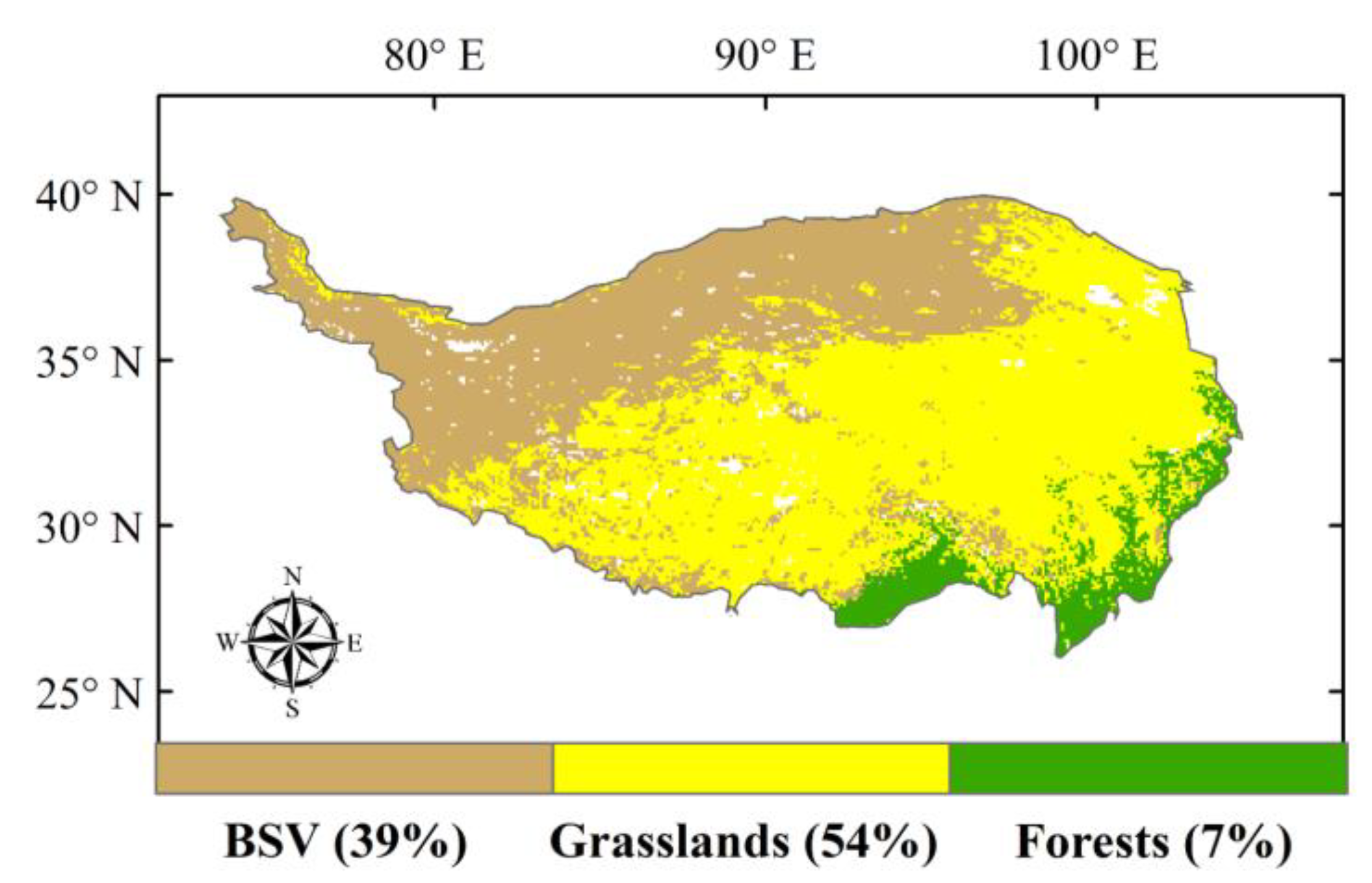
2.3. Land-Cover Data

We used the MODIS land-cover product (MCD12C1) to describe land-cover types of the QTP. This annual product describes the geographic distribution of 17 land-cover types defined by the International Geosphere–Biosphere Programme (IGBP) with a spatial resolution of 0.05° × 0.05° since 2000. To match it with the spatial grid of the ERA5 product presented in Section 2.1, this dataset was resampled by selecting the land-cover types located in the same ERA5 grid cell with the highest appearance frequencies. Given that land cover may change over a long period, the land-cover type with the highest appearance probability during 2000–2021 was assigned for each pixel to minimize the temporal shifts in land-cover types. To this end, appearance probability was estimated using the average of the percentage values affiliated with the MODIS IGBP land-cover product. We further simplified the land-cover classifications (Figure 1), and only three types, i.e., barren or sparsely vegetated areas (BSVs), grasslands, and forests, were used in the following analyses. Other land-cover types, such as croplands and shrublands, whose numbers of available pixels were < 3% were excluded and were not considered in the following analysis.

2.4. Vegetation Sensitivity in Response to Climate Change

Vegetation sensitivity here is defined as the mean state of vegetation per unit increase in climate drivers. To this end, coefficients derived from a multiple linear regression (MLR) model were used to quantify the vegetation sensitivity in response to temperature, solar radiation, and water availability. To disentangle the collinearity impact between the climate driving factors, principal component regression (PCR) [41] was used along with the MLR model, and only principal components with a significant coefficient (p < 0.1) in the PCR were kept in the subsequent analyses. The three climate-driving data were normalized via their Z-scores after they were seasonally detrended by subtracting corresponding climatology, which would increase the robustness of the MLR model used and make the resulting regression coefficients comparable to each other. The key formulation to estimate vegetation sensitivity in response to the three climate factors in each pixel is expressed as follows:
V P = α × T e m p + β × S o l a r + γ × W a t e r + ε
where VP denotes one of the vegetation proxies, including EVI, NDVI, LAI, and SIF; α, β, and γ are regression coefficients that are used as proxies for the vegetation sensitivity in response to temperature (Temp), solar radiation (Solar), and water availability (Water), respectively; and ε denotes residuals.
We advanced the use of the above time-invariant vegetation sensitivity by using a moving-window-based method in a robust way. The interannual vegetation sensitivity was obtained by applying MLR with PCR to anomaly Z-scores of vegetation and climatic datasets for a 5-year moving window advancing by yearly steps over the experimental periods. The investigation period in our work was restricted to the growing season of the QTP, and therefore the available samples included in the 5-year moving time window were generally limited, which may have led to unreliable estimates of regression coefficients. To address this issue, the Moving Block Bootstrap (MBB) approach [46] was considered here to draw blocks of data quadruplets, i.e., a vegetation datum and three climatic data, included in corresponding 5-year windows stochastically. The MBB method can preserve the temporal auto-correlation in time series data by keeping time series for the same year unchanged during the sample-construction process. To guarantee reliable regression coefficients, the resampling procedure was repeated 500 times for each window, and we took an average of the resulting coefficients to obtain a robust estimate of the regression coefficients. In addition, MLR only works when the number of available monthly samples included in a moving window is greater than 10.
The 5-year time window was used here to identify the temporal variability of vegetation sensitivity with relatively sufficient statistical power (the number of available samples was typically > 10), while keeping the kernel size of the window short enough to capture the interannual variability of the vegetation sensitivity. The timeframe of our analysis was from 1 January 2000 to 31 December 2021 for the experiments using LAI, EVI, and NDVI data and began at 1 January 2000 and ended at 31 July 2020 for the SIF data.

2.5. Trend Analysis with the Mann–Kendall Test

Theil–Sen median trend analysis [47] is a robust nonparametric statistical trend calculation method that describes the trend of a long-term data set. The calculation formula is as follows:
β = Median ( X j X i j i ) ,   2000 i   <   j 2021
where β is the slope and Xi and Xj are the target data at time steps i and j, respectively. A positive value for β illustrates an increasing trend, while a negative value indicates a decreasing trend for the target data set.
The Mann–Kendall test is typically combined with the Theil–Sen median estimator to determine the statistical significance of the obtained trend. The merit of the Mann–Kendall test is that it does not require that the target data follow a normal distribution. Readers are recommended to refer to Mann [48] and Kendall [49] for details. Here, these two methods were jointly used to determine the trends and their significance for the vegetation dynamics and the interannual vegetation sensitivity.

3. Results

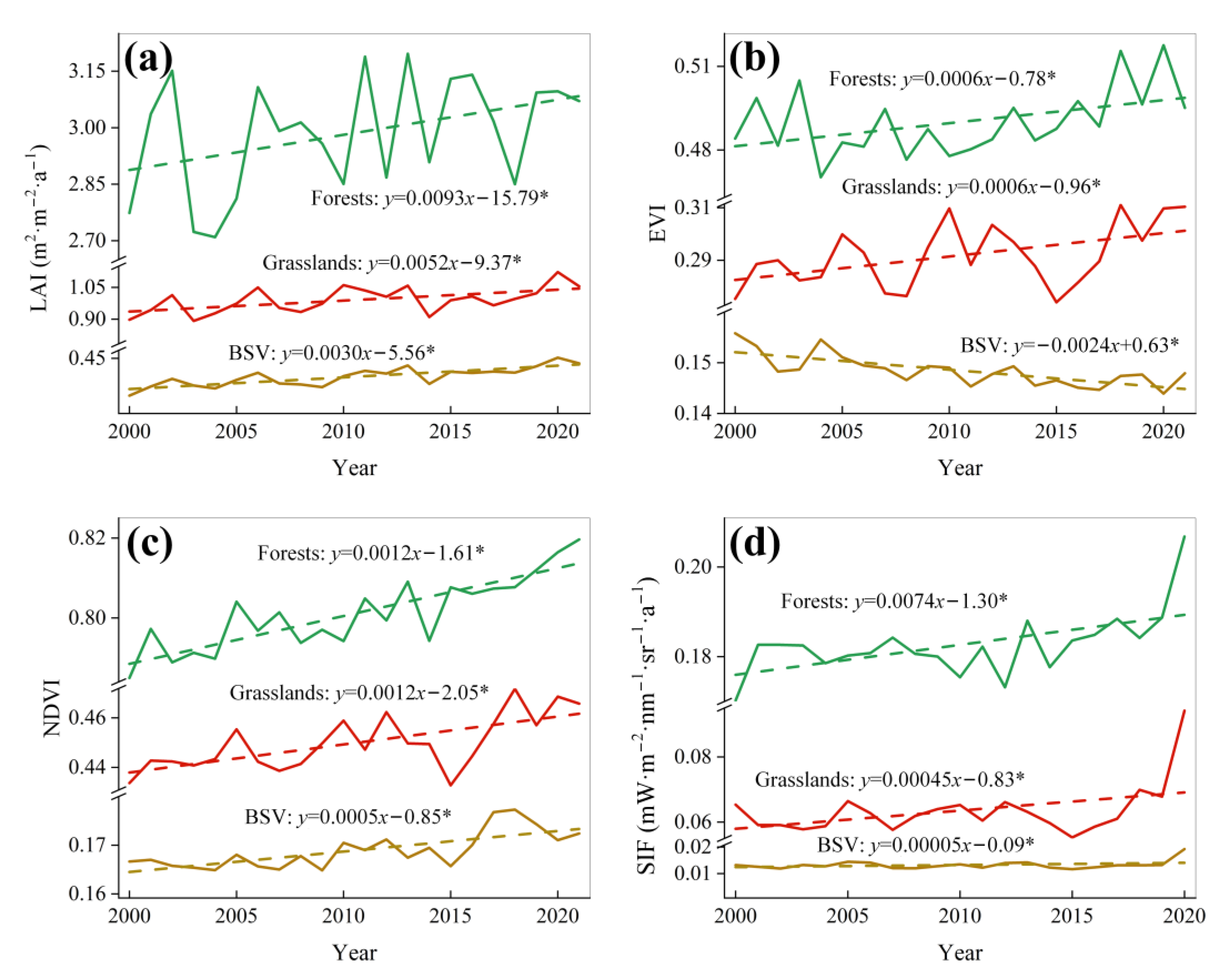
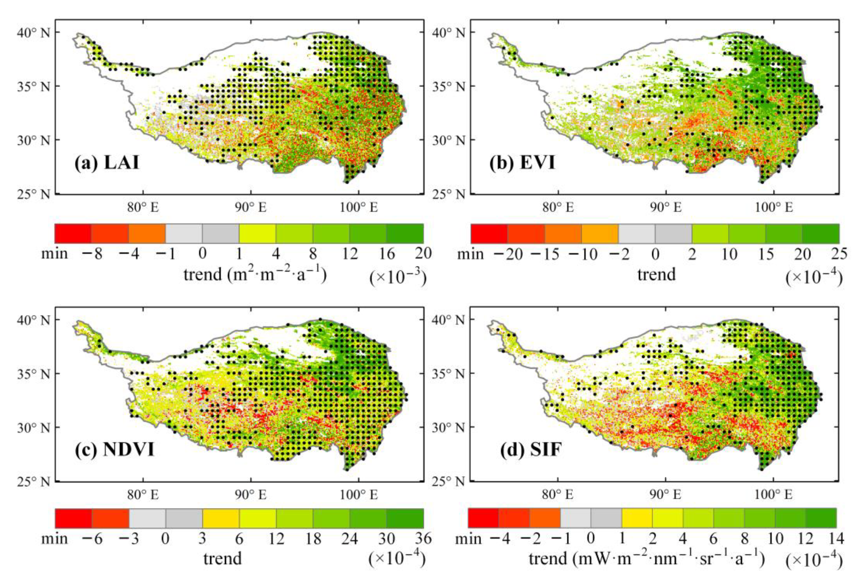
3.1. Interannual Vegetation Dynamics Based on LAI, EVI, NDVI, and SIF Products

This section explores interannual vegetation dynamics of the QTP using LAI, EVI, NDVI, and SIF products. Figure 2 gives an overall picture of the temporal variability of vegetation dynamics for three land-cover types, while Figure 3 presents associated spatial patterns of the vegetation dynamic trends.
Figure 2 demonstrates that the temporal variability of the vegetation dynamics indicated by the four vegetation proxies was similar for the three land-cover types. Overall, all three land-cover types exhibited an upward trend regarding the temporal variability of vegetation dynamics. Only one case exhibited a significant downward trend, i.e., the BSV case described by EVI data, shown in Figure 2b. The trends for all cases were statistically significant except for one case, i.e., the BSV case indicated by SIF data. In general, forests appeared to have the largest upward trend, followed by grasslands and BSVs. It is noticeable in Figure 2d that SIF data appeared to increase substantially in the year 2020. Keep in mind that the SIF data ended at 31 July 2020 and that, consequently, the temporal average was relatively higher than the SIF averages for other years.
Overall, the spatial patterns were similar for the temporal trends of vegetation dynamics indicated by the four vegetation products. Generally, upward trends were observed in 69%, 77%, 79%, and 81% of the total pixels for the EVI, SIF, LAI, and NDVI datasets, respectively. For EVI, NDVI, and SIF data, the upward trends gradually decreased from the eastern to western QTP, and pixels with negative trends were mostly distributed in the southern and southwestern areas of the QTP (Figure 3a–c). By contrast, pixels with negative trends were sparsely distributed in the central to southern areas of the QTP for LAI data (Figure 3d). It is worth mentioning that grasslands located in the southwestern QTP experienced more or less decreasing trends, especially for the results indicated by the SIF data in Figure 3d.
In general, the dotted lines in Figure 4 demonstrate that temperature exhibited an increasing trend, while solar radiation presented a decreasing trend over 2000–2021 on the QTP. The regression coefficients of the fit lines were significant for temperature (Figure 4d) and solar radiation (Figure 4f). By contrast, water availability displayed an insignificant decreasing trend, shown in Figure 4e. Spatially, pixels with significant increasing trend values were clustered in the central to southern QTP for temperature. For solar radiation, as shown in Figure 4c, an insignificant increasing trend was found in western areas, northern areas, and southeastern areas of the QTP. Compared with temperature and solar radiation, water availability exhibited a rather scattered spatial distribution, and no explicit spatial pattern was observed in Figure 4b.

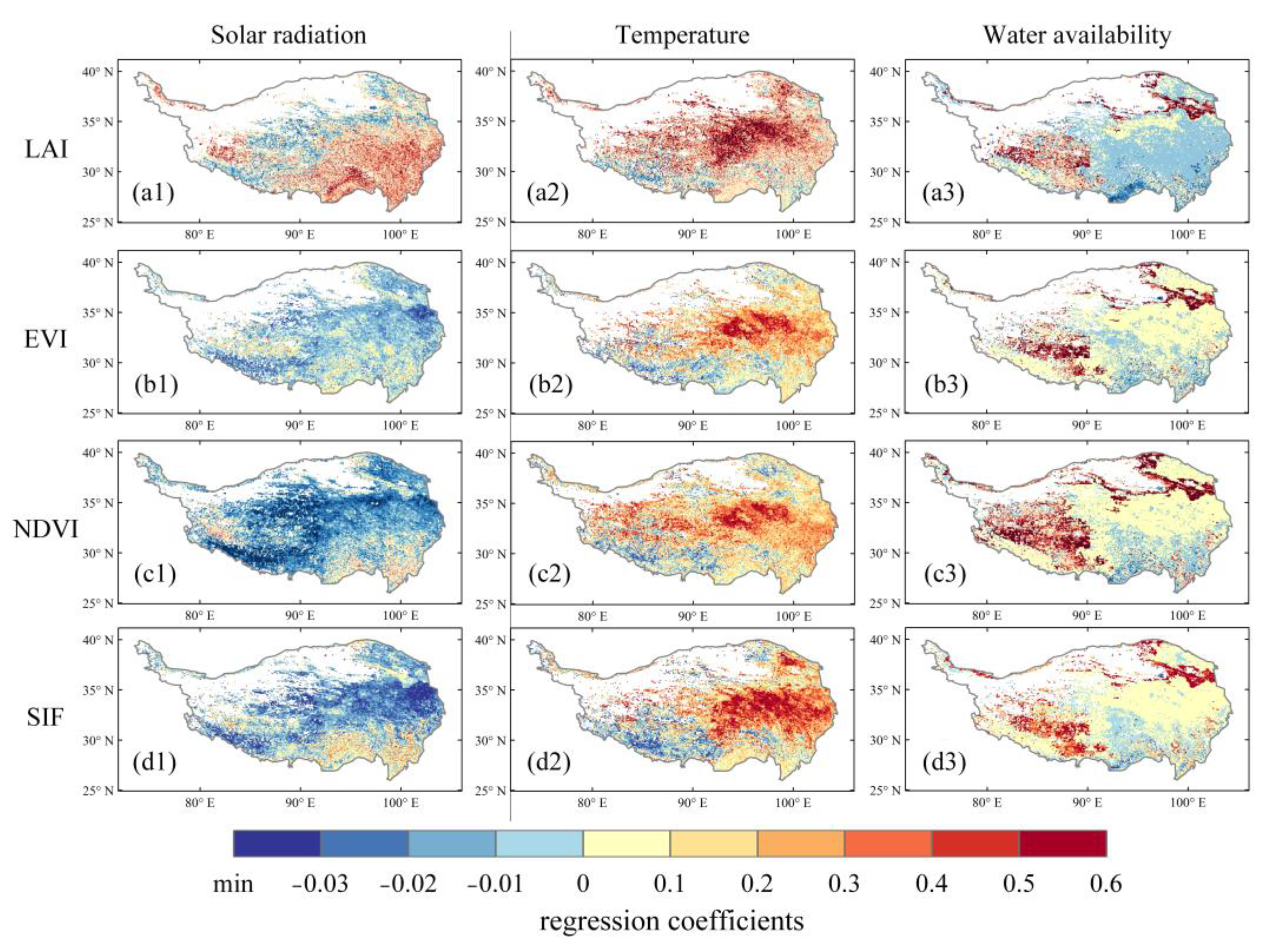
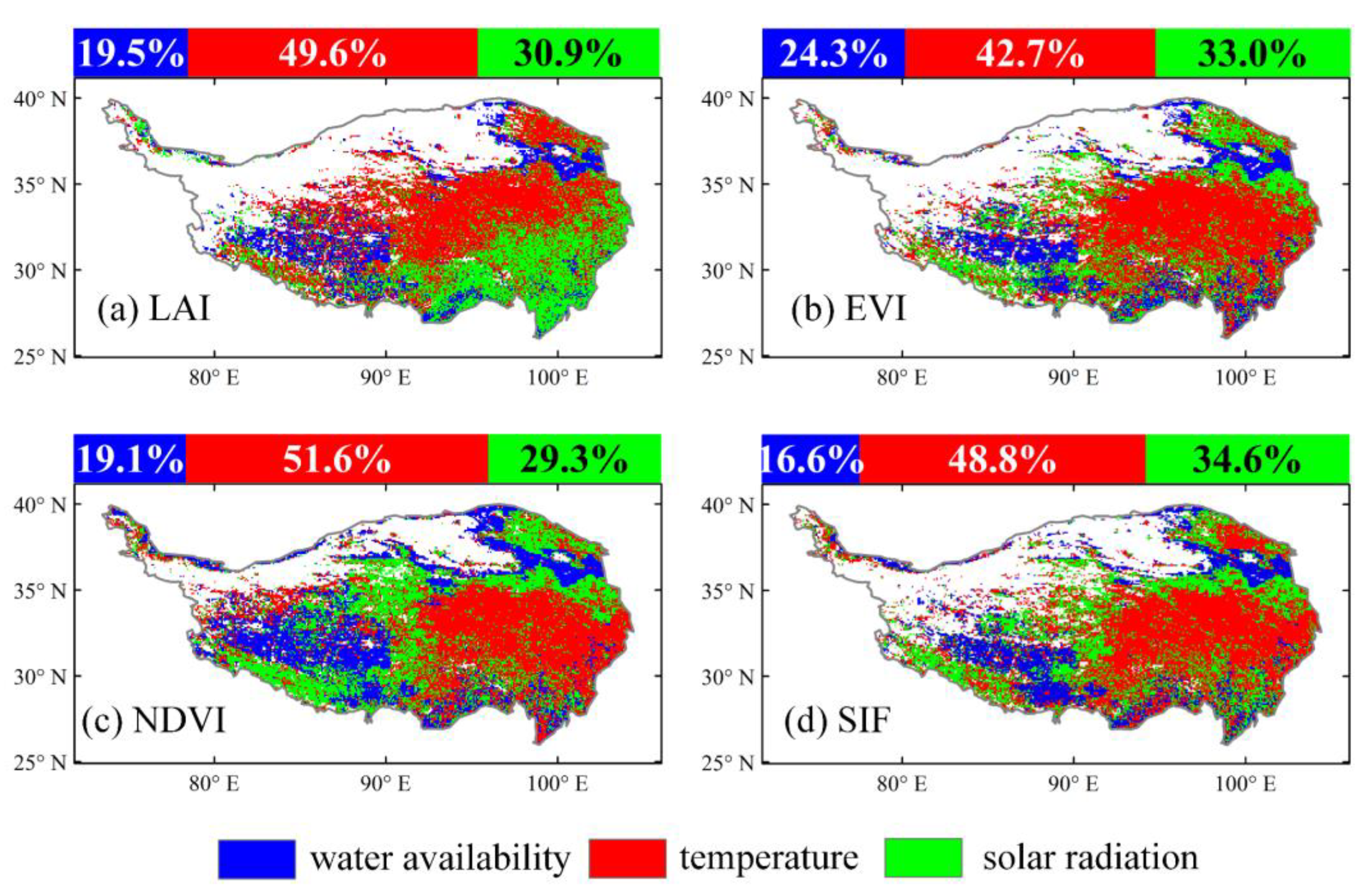
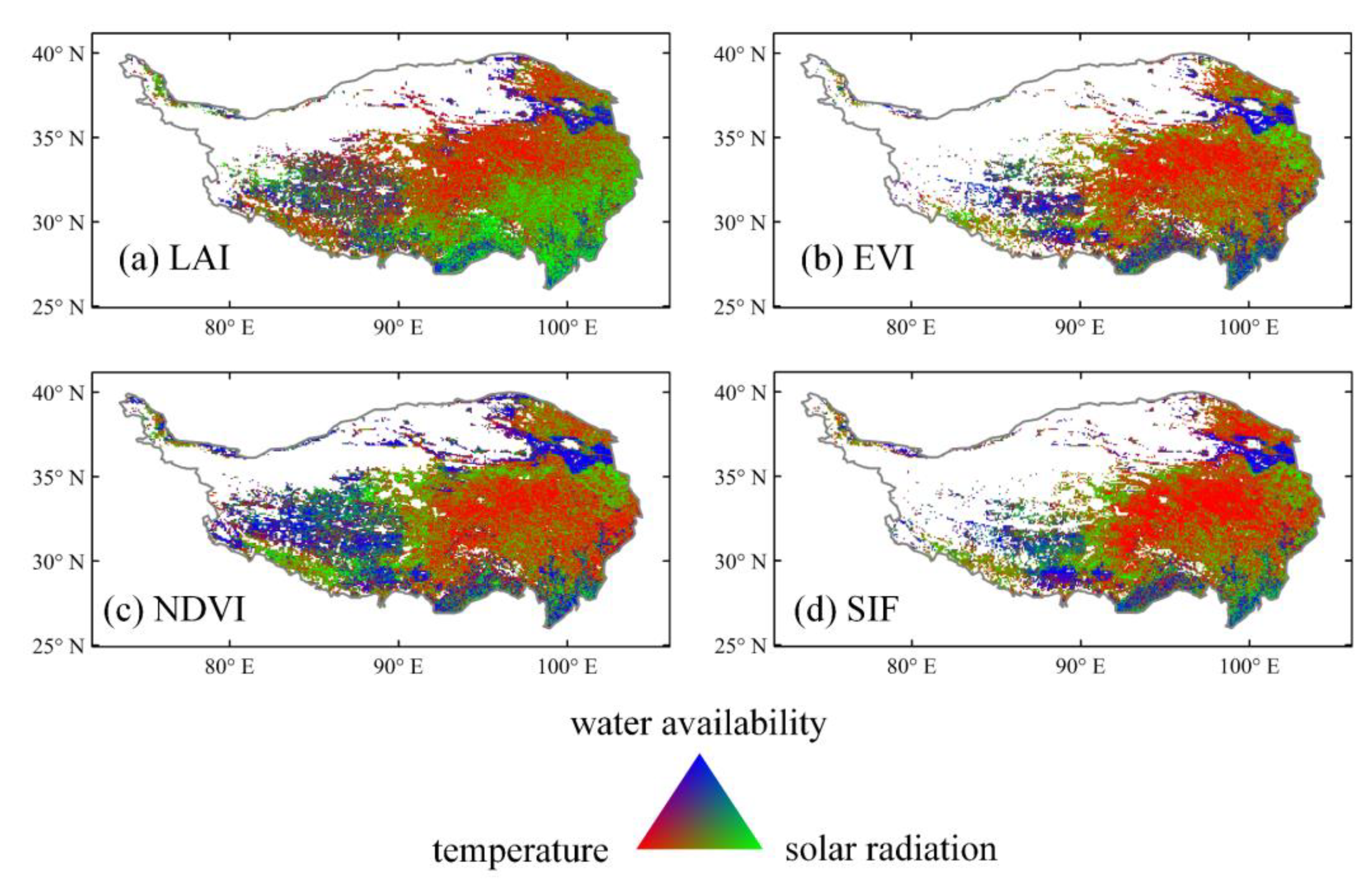
3.2. Time-Invariant Response of Vegetation Dynamics to Climate Changes

Before investigating time-variant vegetation sensitivity, it is necessary to explore time-invariant vegetation sensitivity, as previous related studies have done. In this section, the spatial patterns of time-invariant vegetation sensitivity in response to the three climate factors are investigated (Figure 5) using the obtained regression coefficients. The dominant climate factor with the largest regression coefficient for vegetation sensitivity is revealed in Figure 6.
Except for LAI, the spatial patterns were similar for EVI, NDVI, and SIF products regarding their sensitivity to the three climatic factors. In general, solar radiation had a negative impact on vegetation dynamics, as associated regression coefficients were mostly <0. Positive regression coefficients were found in the southeastern QTP, and associated coefficient values were relatively small (<0.2). Compared with EVI, NDVI, and SIF, LAI displayed a contrasting spatial pattern, as shown in Figure 5, as regression coefficients were relatively large in the southeastern QTP, while they were negative and relatively small in the western QTP. The vegetation sensitivity in response to temperature was similar for all four vegetation products (the second column in Figure 5). Positive regression coefficients were observed in the central to eastern QTP, and associated values were relatively large (>0.3). By contrast, negative regression values were found for parts of regions located in the southwestern QTP. As for water availability, shown in the third column in Figure 5, except for LAI, the other three proxies revealed that their sensitivity to water availability was small, as corresponding values were in a range from −0.1 to 0.1. Relatively large and positive regression coefficients were found in parts of areas distributed in the western and northeastern QTP. Nevertheless, LAI indicated that negative regression values (>−0.1) were observed for most pixels in southern and central-to-eastern areas of the QTP.
The four vegetation proxies in Figure 6 jointly reveal that temperature was the most important factor regulating vegetation sensitivity on the QTP, followed by solar radiation and water availability. Temperature was the dominant factor in 49.6%, 42.7%, 51.6%, and 48.8% of the total pixels for LAI, EVI, NDVI, and SIF data, respectively. Solar radiation and water availability were identified as the dominant factors in about 30% and 20% of total pixels, respectively. The spatial patterns of the dominant climatic factors were similar for EVI, NDVI, and SIF proxies, while a relatively different spatial pattern was observed for LAI data. EVI, NDVI, and SIF data jointly exhibited that temperature was the dominant factor for pixels located in the central to eastern QTP. Water availability was the dominant factor for pixels distributed in parts of areas of the southwestern and northeastern QTP. Pixels with solar radiation as the dominant factor were sparsely distributed on the QTP, and most of them were found in the northeastern and western QTP. Nevertheless, LAI suggested that solar radiation was the dominant factor for pixels located in the southeastern QTP.

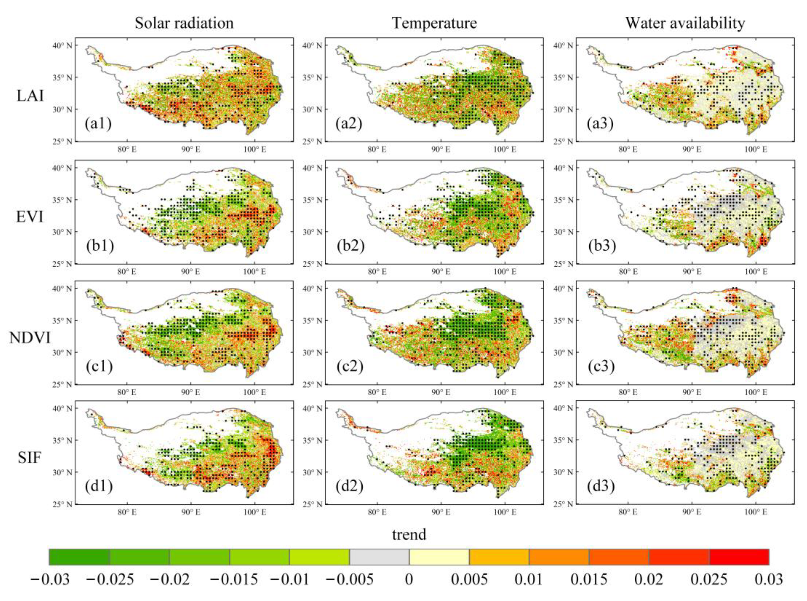
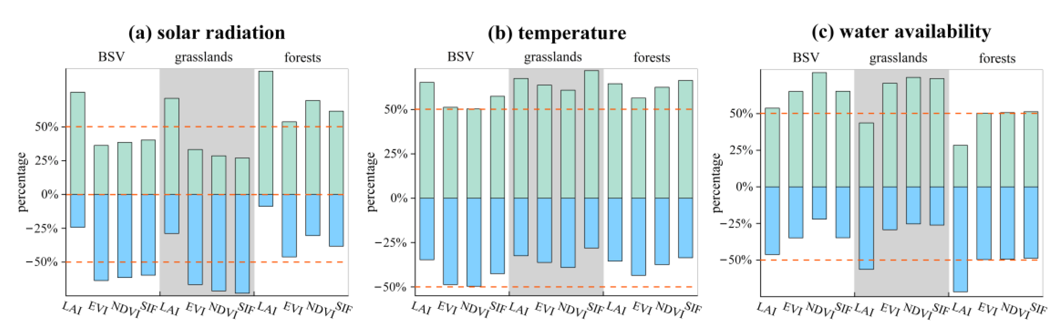
3.3. Time-Variant Response of Vegetation Dynamics to Climate Changes

Section 3.2 only explores the time-invariant vegetation sensitivity in response to the three climate factors; the temporal variability of the vegetation sensitivity could not be determined. This section focuses on the time-variant vegetation sensitivity with a view to investigating the spatial patterns of its temporal trends (Figure 7), the trend values classified by land-cover types (Figure 8), the impact directions indicated by the signs of regression coefficients (Figure 9), and associated dominant climate factors (Figure 10).
Overall, Figure 7 illustrates that the spatial patterns were similar for the trend values of vegetation sensitivity in response to the three climatic factors, as indicated by the LAI, EVI, NDVI, and SIF data. The vegetation sensitivity displayed a significant upward trend in response to solar radiation in eastern and parts of southern areas of the QTP, while a significant downward trend in central areas of the QTP was observed. Vegetation sensitivity in response to temperature exhibited a significant downward trend in the central to northeastern QTP. Conversely, pixels with an upward trend were sparsely distributed in other regions and did not yield explicit spatial patterns. Compared with temperature and solar radiation, vegetation exhibited a much lower trend regarding the sensitivity in response to water availability, as most of the associated trend values were in a range from −0.005 to 0.005. Nevertheless, trend values of water availability were noticeable in the southwestern QTP, as trend values of associated pixels were typically >0.05 or <−0.05.
The boxplots in Figure 8 demonstrate that the trend of vegetation sensitivity in response to the three climatic factors was generally consistent for the four vegetation proxies when considering different land-cover types. As indicated by all four vegetation proxies, vegetation sensitivity in response to temperature gradually decreased over the recent two decades in BSVs, grasslands, and forests, as the associated means and medians of the trend values were <0 (Figure 8b). Such decreasing trends were more pronounced in grasslands than in BSVs and forests. Except for the LAI case, shown in Figure 8a, vegetation sensitivity in response to solar radiation experienced a decreasing trend for BSVs and grasslands. By contrast, an increasing sensitivity was found for forests areas, except for the EVI case. For water availability, as shown in Figure 8c, only the forest cases indicated by SIF data yielded a contrasting trend, i.e., mean and median metrics indicated different trend directions, when compared with the other three proxies. BSVs and forests showed increasing trends, while no obvious trend could be determined for the grasslands, as corresponding mean and median values were typically small and indicated different directions.
Given that a climate factor may exert an opposite impact on the vegetation sensitivity over the investigation period, which could not be revealed in Figure 7 and Figure 8, we further investigated the signs of the regression coefficients classified by the three land-cover types, as represented in Figure 9.
In general, the boxplots in Figure 9a show that solar radiation exerted a negative impact on vegetation in BSVs and grasslands, while it exerted a positive impact on vegetation in forests. Figure 9b illustrates that temperature generally had a negative impact on all three land-cover types. By contrast, water availability displayed a positive impact on BSVs and grasslands (Figure 9c). Nevertheless, no obvious sign of the regression coefficients could be determined for forests. Taking all four vegetation proxies into consideration, we further summarized the trend of vegetation sensitivity illustrated in Figure 8 and corresponding signs of the regression coefficients displayed in Figure 9. The conclusions are shown in Table 1.
The dominant climate factor that exerted the largest impact on vegetation sensitivity was revealed by comparing the absolute values of the regression coefficients for the three climatic driving factors for each year. For a given pixel in a given year, the climate factor with the maximum regression coefficient was regarded as the dominant factor. The fraction values describing the appearance frequency for each climate factor over the whole investigation period were calculated and were RGB-composited, as shown in Figure 10.
A distinct spatial pattern was observed for the dominant climatic factor with respect to regulation of the time-variant vegetation sensitivity shown in Figure 10, which was strongly consistent with the spatial pattern of the time-invariant vegetation sensitivity shown in Figure 6. LAI exhibited a relatively different spatial pattern, as solar radiation was found to exert the maximum impact on vegetation sensitivity in the southeastern QTP. Conversely, EVI, NDVI, and SIF jointly revealed that temperature and water availability controlled the vegetation sensitivity in the southeastern QTP. In general, temperature was the dominant factor for pixels located in the central to eastern QTP. Water availability was the dominant factor for pixels located in the northeastern QTP and forest areas in the southern QTP, which findings were different in comparison with the time-invariant vegetation sensitivity shown in Figure 6. The spatial pattern of solar radiation was relatively scattered, and the corresponding pixels were mostly distributed around the spatial distribution of temperature factors.

4. Discussion

Overall, the trend values indicated by the four vegetation proxies appeared to show similar change patterns, indicating a strong consistency among different data sources in capturing the temporal variability of vegetation on the QTP. All the data demonstrate that vegetation on the QTP has been greening in the last two decades, as about 70–80% of the total pixels indicated an upward trend [6,24,38,50]. In the context of global warming and increasing emissions of carbon dioxide, vegetation activity on the QTP has enhanced substantially [51]. Carbon dioxide is known to stimulate vegetation growth through the combined effects of the direct physiological effect and the indirect effect of climate change induced by itself [52]. Consequently, these two factors contribute to favorable conditions for vegetation growth on the QTP and result in the greening phenomenon observed. It has to be stressed that EVI, NDVI, and LAI data more or less indicate that vegetation located in the southwestern QTP is browning [50,51,53]. Nevertheless, this phenomenon is more predominant, as indicated by the SIF data. Such phenomena arouse particular concern for associated vegetation, since SIF is reported to be more correlated with vegetation photosynthesis activity than vegetation index [8,54]. Moreover, the biodiversity of the QTP will decrease in future if global warming is not curbed [55]. This would make vegetation in the southwestern QTP more vulnerable in the near future and needs special attention.
Time-invariant and time-variant vegetation sensitivity derived from LAI data were relatively different when compared with those obtained from the other three vegetation proxies. Pixels with such discrepancies were mainly found in the southeastern QTP, where forests account for a large proportion of the land cover. Although EVI, NDVI, and SIF can well capture the seasonal variability of LAI, they are reported to provide premature estimates of the onset of the growing season in forests [56]. Moreover, the relationship between LAI and vegetation index is found to change with the leaf seasonality, leaf orientation, and growth stage of vegetation cover [57]. These factors may lead to the different performance of LAI in comparison with EVI, NDVI, and SIF.
As a vegetation proxy that is drawing more and more attention, SIF has an evaluation performance highly consistent with those of NDVI and EVI. Different from NDVI, EVI, and LAI, SIF is directly linked to photosynthetic activity and has an advantage over vegetation indices in describing plant physiological responses to water stress [54,58]. In addition, SIF is more sensitive to climate variables than vegetation indices [59] and shows a premature start of season relative to the vegetation index [60]. Consequently, SIF is expected to have a different performance to the other three vegetation proxies. However, keep in mind that a monthly time scale was considered here and that SIF values included in the same month were averaged in our analysis. Such processing conceals the characteristics of the high temporal resolution, e.g., 4 days, in SIF data, resulting in SIF having a similar performance to EVI and NDVI data here.
Vegetation sensitivity in response to climate change exhibited pronounced spatiotemporal heterogeneity on the QTP for the four vegetation proxies. For both time-invariant and time-variant sensitivity, temperature was the most important factor regulating vegetation sensitivity of the QTP over the last two decades, which is consistent with the findings of Piao et al. [1], Lin et al. [2], Zhang et al. [6], and Ma et al. [24]. Our results revealed that temperature generally exerted positive impacts on vegetation sensitivity for the high-cold grasslands located in the central to eastern QTP, which was also reported in the study by Fu and Sun [61]. However, our results also demonstrated that vegetation of the QTP experienced a downward trend in the sensitivity to temperature variability, indicating that the impact of temperature on vegetation is gradually decreasing. In particular, Zhu et al. [62] pointed out that such declining phenomena reflect a shift from water to energy limitations for vegetation of the QTP. Moreover, the declining trend may be attributed to the acclimation of plants and communities, such as plant biomass allocation and changes in community composition, so that vegetation on the QTP [63,64,65] can cope with the widespread global warming.
We found solar radiation to be an important climate factor that should not be ignored in vegetation sensitivity studies, which has also been emphasized recently by Zhang et al. [22], Ma et al. [24], and Jiang et al. [37]. The trend analysis showed that forests in the southeastern QTP displayed an increasing sensitivity to solar radiation. As temperature is continuously increasing in the southeastern QTP [6], solar radiation modifies forest sensitivity by stimulating photosynthesis and makes forests absorb more carbon dioxide. By contrast, grasslands and BSVs appeared to show declining sensitivity in response to solar radiation, and solar radiation exerted negative impacts on grasslands and BSVs. This may be explained by the fact that high levels of solar radiation on the QTP make plants reach their light saturation points easily by regulating leaf nitrogen and phosphorus stoichiometry, which leads to the photoinhibition of photosynthesis [66].
Compared with temperature and solar radiation, all four vegetation proxies revealed a small temporal trend for vegetation sensitivity in response to water availability on the QTP in the last two decades. Such phenomena were more pronounced in central to eastern areas of the QTP, where the trend values for grasslands were small, which may be explained by their elevations. By contrast, forests and BSVs exhibited upward trends regarding water availability, which is consistent with the findings of Wang et al. [65] and Li et al. [17] and may be related to the human–environment nexus [13] through grazing, farming, and urbanization [50]. Over the last two decades, water availability generally exerted positive impacts on vegetation sensitivity, except for the forests located in the southeastern QTP. Forested areas are more sensitive to water availability than temperature and solar radiation, and they displayed positive sensitivity trends. This may occur as a consequence of climate warming and persistent drought in these areas [67,68]. In addition, Shen et al. [4] pointed out that precipitation impacts on vegetation spring phenology on the QTP, especially in the drylands, which may alter the vegetation sensitivity on the QTP accordingly.
As the temperature of the QTP is expected to continuously increase in the future, the vegetation sensitivity of the grasslands located in the central QTP may experience an intensified increase in vegetation sensitivity, as our results revealed that temperature is the main climate factor dominating vegetation sensitivity in these areas. In the future, grasslands having a high vegetation sensitivity means that the grassland ecosystem of the QTP will become more vulnerable, and the situation may become even worse if humans relax protection efforts. In forests located in the southeastern QTP, more attention should be paid to the temporal variability in water availability and solar radiation, since these two factors are the dominant climate factors regulating the vegetation sensitivity of forests in these regions.
There are two limitations to our study. First, only the first-order moment, i.e., the mean state, indicated by regression coefficients derived from MLR was considered. The second-order moment indicated by variance metrics, such as the Vegetation Sensitivity Index (VSI) proposed by Seddon et al. [41], was ignored. Nevertheless, the first and second moments describe vegetation sensitivity in response to climate change from different perspectives, and our results, e.g., the dominant climate factors, may change when considering VSI metrics. Second, the window size was set as 5 years, which is significantly smaller than the 15-year window used in the studies of Chen et al. [69] and Jiang et al. [37]. However, studies such as Zeng et al.’s [36] and Wang et al.’s [38] also applied a moving time window with a kernel size of 5 years, and they reported that changing the window size would result in strongly consistent trend results for the regression coefficients, which needs further investigation.

5. Conclusions

We investigated time-invariant and time-variant (interannual) vegetation sensitivity in response to temperature, solar radiation, and water availability on the QTP over the last two decades by considering four vegetation proxies, including LAI, EVI, NDVI, and SIF products. Except for LAI, the other three vegetation proxies provided strongly consistent evaluations regarding the interannual vegetation dynamics and vegetation sensitivity in response to climate change. Overall, the vegetation dynamics indicated by the four vegetation products all showed increasing trends over the last two decades, as pixels with an upward trend value accounted for 69%, 77%, 79%, and 81% of the total pixels for the EVI, SIF, LAI, and NDVI data, respectively. The greening trend gradually decreased from the eastern to western QTP, and pixels with a negative trend were clustered in southern and southwestern areas of the QTP. Compared with those of the other three vegetation proxies, SIF data indicated a widespread decreasing trend for grasslands located in the southwestern QTP.
Trend analysis revealed that temperature exerted positive impacts on vegetation, but vegetation of the QTP displayed a decreasing sensitivity to temperature. Solar radiation was shown to have a positive impact on forests, while it had negative impacts on grasslands and BSVs. Grasslands and BSVs exhibited decreasing sensitivity, while forests showed increasing sensitivity to solar radiation. As for water availability, forests and BSVs exhibited increasing sensitivity, but no obvious trend was observed for grasslands. Water availability exerted positive impacts on grasslands and BSVs, and no obvious impact direction could be determined for forests. The spatial patterns of the dominant climate factors were similar for time-invariant and time-variant vegetation sensitivity. In general, temperature is the most important driving factor, followed by solar radiation and water availability. Temperature and solar radiation jointly dominated the vegetation sensitivity in central to eastern areas of the QTP. By contrast, water availability was the dominant factor regarding vegetation sensitivity in forests in the southeastern QTP and in grasslands in northeastern and southwestern areas of the QTP. Our findings have important implications for understanding response and feedback associated with climate change in the vegetation dynamics on the QTP, providing a baseline for vegetation preservation and management for policymakers.

Author Contributions

Conceptualization, K.W. and Z.H.; methodology, K.W.; software, K.W.; formal analysis, H.Y.; investigation, J.C.; resources, K.W.; data curation, Y.Y.; writing—original draft preparation, K.W. and J.C.; writing—review and editing, K.W. and H.Y.; visualization, Y.Y.; supervision, K.W. and Z.H.; project administration, K.W., Y.Y. and Z.H.; funding acquisition, K.W., Y.Y. and Z.H. All authors have read and agreed to the published version of the manuscript.

Funding

This research was funded by the Second Tibetan Plateau Scientific Expedition and Research Program (2019QZKK0405), the Hainan Provincial Natural Science Foundation of China (623RC447, 423QN208), and the Hainan University start-up fund (KYQD(ZR)-22084, KYQD(ZR)21096, RZ2200001144). Key RGD Program of Hainan (ZDYF2022SHFZ042).

Data Availability Statement

The data presented in this study are available on request from the corresponding author.

Conflicts of Interest

The authors declare no conflict of interest.

References

  1. Piao, S.; Cui, M.; Chen, A.; Wang, X.; Ciais, P.; Liu, J.; Tang, Y. Altitude and Temperature Dependence of Change in the Spring Vegetation Green-up Date from 1982 to 2006 in the Qinghai-Xizang Plateau. Agric. For. Meteorol. 2011, 151, 1599–1608. [Google Scholar] [CrossRef]
  2. Lin, X.; Zhang, Z.; Wang, S.; Hu, Y.; Xu, G.; Luo, C.; Chang, X.; Duan, J.; Lin, Q.; Xu, B.; et al. Response of Ecosystem Respiration to Warming and Grazing during the Growing Seasons in the Alpine Meadow on the Tibetan Plateau. Agric. For. Meteorol. 2011, 151, 792–802. [Google Scholar] [CrossRef]
  3. Yao, T.; Wu, F.; Ding, L.; Sun, J.; Zhu, L.; Piao, S.; Deng, T.; Ni, X.; Zheng, H.; Ouyang, H. Multispherical Interactions and Their Effects on the Tibetan Plateau’s Earth System: A Review of the Recent Researches. Natl. Sci. Rev. 2015, 2, 468–488. [Google Scholar] [CrossRef] [Green Version]
  4. Shen, M.; Piao, S.; Cong, N.; Zhang, G.; Jassens, I.A. Precipitation Impacts on Vegetation Spring Phenology on the Tibetan Plateau. Glob. Change Biol. 2015, 21, 3647–3656. [Google Scholar] [CrossRef] [Green Version]
  5. Xu, B.; Cao, J.; Hansen, J.; Yao, T.; Joswia, D.R.; Wang, N.; Wu, G.; Wang, M.; Zhao, H.; Yang, W.; et al. Black Soot and the Survival of Tibetan Glaciers. Proc. Natl. Acad. Sci. USA 2009, 106, 22114–22118. [Google Scholar] [CrossRef] [PubMed] [Green Version]
  6. Zhang, L.; Guo, H.D.; Wang, C.Z.; Ji, L.; Li, J.; Wang, K.; Dai, L. The Long-Term Trends (1982–2006) in Vegetation Greenness of the Alpine Ecosystem in the Qinghai-Tibetan Plateau. Environ. Earth Sci. 2014, 72, 1827–1841. [Google Scholar] [CrossRef]
  7. Peltier, D.M.P.; Ogle, K. Tree Growth Sensitivity to Climate Is Temporally Variable. Ecol. Lett. 2020, 23, 1561–1572. [Google Scholar] [CrossRef]
  8. Xie, X.; He, B.; Guo, L.; Huang, L.; Hao, X.; Zhang, Y.; Liu, X.; Tang, R.; Wang, S. Revisiting Dry Season Vegetation Dynamics in the Amazon Rainforest Using Different Satellite Vegetation Datasets. Agric. For. Meteorol. 2022, 312, 108704. [Google Scholar] [CrossRef]
  9. Jin, J.; Wang, Q. Assessing Ecological Vulnerability in Western China Based on Time-Integrated NDVI Data. J. Arid. Land 2016, 8, 533–545. [Google Scholar] [CrossRef] [Green Version]
  10. Gao, J.; Jiao, K.; Wu, S. Quantitative Assessment of Ecosystem Vulnerability to Climate Change: Methodology and Application in China. Environ. Res. Lett. 2018, 13, 094016. [Google Scholar] [CrossRef]
  11. Li, K.; Tong, Z.; Liu, X.; Zhang, J.; Tong, S. Quantitative Assessment and Driving Force Analysis of Vegetation Drought Risk to Climate Change:Methodology and Application in Northeast China. Agric. For. Meteorol. 2020, 282–283, 107865. [Google Scholar] [CrossRef]
  12. He, L.; Guo, J.; Yang, W.; Jiang, Q.; Chen, L.; Tang, K. Multifaceted Responses of Vegetation to Average and Extreme Climate Change over Global Drylands. Sci. Total Environ. 2023, 858, 159942. [Google Scholar] [CrossRef] [PubMed]
  13. Abel, C.; Horion, S.; Tagesson, T.; De Keersmaecker, W.; Seddon, A.W.R.; Abdi, A.M.; Fensholt, R. The Human–Environment Nexus and Vegetation–Rainfall Sensitivity in Tropical Drylands. Nat. Sustain. 2021, 4, 25–32. [Google Scholar] [CrossRef]
  14. Yuan, X.; Hamdi, R.; Ochege, F.U.; Kurban, A.; De Maeyer, P. The Sensitivity of Global Surface Air Temperature to Vegetation Greenness. Int. J. Climatol. 2020, 41, 483–496. [Google Scholar] [CrossRef]
  15. You, G.; Liu, B.; Zou, C.; Li, H.; McKenzie, S.; He, Y.; Gao, J.; Jia, X.; Altaf Arain, M.; Wang, S.; et al. Sensitivity of Vegetation Dynamics to Climate Variability in a Forest-Steppe Transition Ecozone, North-Eastern Inner Mongolia, China. Ecol. Indic. 2021, 120, 106833. [Google Scholar] [CrossRef]
  16. Zhang, Q.; Yuan, R.; Singh, V.P.; Xu, C.Y.; Fan, K.; Shen, Z.; Wang, G.; Zhao, J. Dynamic Vulnerability of Ecological Systems to Climate Changes across the Qinghai-Tibet Plateau, China. Ecol. Indic. 2022, 134, 108483. [Google Scholar] [CrossRef]
  17. Li, W.; Migliavacca, M.; Forkel, M.; Denissen, J.M.C.; Reichstein, M.; Yang, H.; Duveiller, G.; Weber, U.; Orth, R. Widespread Increasing Vegetation Sensitivity to Soil Moisture. Nat. Commun. 2022, 13, 3959. [Google Scholar] [CrossRef]
  18. Bao, Z.; Zhang, J.; Wang, G.; Guan, T.; Jin, J.; Liu, Y.; Li, M.; Ma, T. The Sensitivity of Vegetation Cover to Climate Change in Multiple Climatic Zones Using Machine Learning Algorithms. Ecol. Indic. 2021, 124, 107443. [Google Scholar] [CrossRef]
  19. Chen, Z.; Liu, H.; Xu, C.; Wu, X.; Liang, B.; Cao, J.; Chen, D. Modeling Vegetation Greenness and Its Climate Sensitivity with Deep-Learning Technology. Ecol. Evol. 2021, 11, 7335–7345. [Google Scholar] [CrossRef]
  20. Chen, B.; Chen, H.; Li, M.; Fiedler, S.; Mărgărint, M.C.; Nowak, A.; Wesche, K.; Tietjen, B.; Wu, J. Climate Sensitivity of the Arid Scrublands on the Tibetan Plateau Mediated by Plant Nutrient Traits and Soil Nutrient Availability. Remote Sens. 2022, 14, 4601. [Google Scholar] [CrossRef]
  21. Li, L.; Zhang, Y.; Wu, J.; Li, S.; Zhang, B.; Zu, J.; Zhang, H.; Ding, M.; Paudel, B. Increasing Sensitivity of Alpine Grasslands to Climate Variability along an Elevational Gradient on the Qinghai-Tibet Plateau. Sci. Total Environ. 2019, 678, 21–29. [Google Scholar] [CrossRef] [PubMed]
  22. Zhang, Q.; Kong, D.; Shi, P.; Singh, V.P.; Sun, P. Vegetation Phenology on the Qinghai-Tibetan Plateau and Its Response to Climate Change (1982–2013). Agric. For. Meteorol. 2018, 248, 408–417. [Google Scholar] [CrossRef]
  23. Wang, Y.; Lv, W.; Xue, K.; Wang, S.; Zhang, L.; Hu, R.; Zeng, H.; Xu, X.; Li, Y.; Jiang, L.; et al. Grassland Changes and Adaptive Management on the Qinghai–Tibetan Plateau. Nat. Rev. Earth Environ. 2022, 3, 668–683. [Google Scholar] [CrossRef]
  24. Ma, M.; Yuan, W.; Dong, J.; Zhang, F.; Cai, W.; Li, H. Large-Scale Estimates of Gross Primary Production on the Qinghai-Tibet Plateau Based on Remote Sensing Data. Int. J. Digit. Earth 2018, 11, 1166–1183. [Google Scholar] [CrossRef]
  25. Sun, B.; Jiang, M.; Han, G.; Zhang, L.; Zhou, J.; Bian, C.; Du, Y.; Yan, L.; Xia, J. Experimental Warming Reduces Ecosystem Resistance and Resilience to Severe Flooding in a Wetland. Sci. Adv. 2022, 8, eabl9526. [Google Scholar] [CrossRef]
  26. Berdugo, M.; Delgado-Baquerizo, M.; Soliveres, S.; Hernández-Clemente, R.; Zhao, Y.; Gaitán, J.J.; Gross, N.; Saiz, H.; Maire, V.; Lehman, A.; et al. Global Ecosystem Thresholds Driven by Aridity. Science 2020, 367, 787–790. [Google Scholar] [CrossRef] [Green Version]
  27. Wigneron, J.P.; Fan, L.; Ciais, P.; Bastos, A.; Brandt, M.; Chave, J.; Saatchi, S.; Baccini, A.; Fensholt, R. Tropical Forests Did Not Recover from the Strong 2015–2016 El Niño Event. Sci. Adv. 2020, 6, eaay4603. [Google Scholar] [CrossRef] [Green Version]
  28. Armenteras, D.; Dávalos, L.M.; Barreto, J.S.; Miranda, A.; Hernández-Moreno, A.; Zamorano-Elgueta, C.; González-Delgado, T.M.; Meza-Elizalde, M.C.; Retana, J. Fire-Induced Loss of the World’s Most Biodiverse Forests in Latin America. Sci. Adv. 2021, 7, eabd3357. [Google Scholar] [CrossRef]
  29. Oliveira, B.F.; Moore, F.C.; Dong, X. Biodiversity Mediates Ecosystem Sensitivity to Climate Variability. Commun. Biol. 2022, 5, 628. [Google Scholar] [CrossRef]
  30. Macdougall, A.S.; McCann, K.S.; Gellner, G.; Turkington, R. Diversity Loss with Persistent Human Disturbance Increases Vulnerability to Ecosystem Collapse. Nature 2013, 494, 86–89. [Google Scholar] [CrossRef]
  31. Yao, Y.; Liu, Y.; Wang, Y.; Fu, B. Greater Increases in China’s Dryland Ecosystem Vulnerability in Drier Conditions than in Wetter Conditions. J. Environ. Manag. 2021, 291, 112689. [Google Scholar] [CrossRef] [PubMed]
  32. Yuan, Y.; Bao, A.; Liu, T.; Zheng, G.; Jiang, L.; Guo, H.; Jiang, P.; Yu, T.; De Maeyer, P. Assessing Vegetation Stability to Climate Variability in Central Asia. J. Environ. Manag. 2021, 298, 113330. [Google Scholar] [CrossRef] [PubMed]
  33. Jiang, L.; Liu, B.; Yuan, Y. Quantifying Vegetation Vulnerability to Climate Variability in China. Remote Sens. 2022, 14, 3491. [Google Scholar] [CrossRef]
  34. Zhang, Y.; Gentine, P.; Luo, X.; Lian, X.; Liu, Y.; Zhou, S.; Michalak, A.M.; Sun, W.; Fisher, J.B.; Piao, S.; et al. Increasing Sensitivity of Dryland Vegetation Greenness to Precipitation Due to Rising Atmospheric CO2. Nat. Commun. 2022, 13, 4875. [Google Scholar] [CrossRef]
  35. Hua, T.; Zhao, W.; Cherubini, F.; Hu, X.; Pereira, P. Sensitivity and Future Exposure of Ecosystem Services to Climate Change on the Tibetan Plateau of China. Landsc. Ecol. 2021, 36, 3451–3471. [Google Scholar] [CrossRef]
  36. Zeng, X.; Hu, Z.; Chen, A.; Yuan, W.; Hou, G.; Han, D.; Liang, M.; Di, K.; Cao, R.; Luo, D. The Global Decline in the Sensitivity of Vegetation Productivity to Precipitation from 2001 to 2018. Glob. Change Biol. 2022, 28, 6823–6833. [Google Scholar] [CrossRef]
  37. Jiang, P.; Ding, W.; Yuan, Y.; Ye, W.; Mu, Y. Interannual Variability of Vegetation Sensitivity to Climate in China. J. Environ. Manag. 2022, 301, 113768. [Google Scholar] [CrossRef]
  38. Wang, S.; Zhang, Y.; Ju, W.; Chen, J.M.; Ciais, P.; Cescatti, A.; Sardans, J.; Janssens, I.A.; Wu, M.; Berry, J.A.; et al. Recent Global Decline of CO2 Fertilization Effects on Vegetation Photosynthesis. Science 2020, 370, 1295–1300. [Google Scholar] [CrossRef]
  39. Wang, Q.; Ju, Q.; Wang, Y.; Fu, X.; Zhao, W.; Du, Y.; Jiang, P.; Hao, Z. Regional Patterns of Vegetation Dynamics and Their Sensitivity to Climate Variability in the Yangtze River Basin. Remote Sens. 2022, 14, 5623. [Google Scholar] [CrossRef]
  40. Hersbach, H.; Bell, B.; Berrisford, P.; Hirahara, S.; Horányi, A.; Nicolas, J.; Peubey, C.; Radu, R.; Bonavita, M.; Dee, D.; et al. The ERA5 Global Reanalysis. Q. J. R. Meteorol. Soc. 2020, 146, 1999–2049. [Google Scholar] [CrossRef]
  41. Seddon, A.W.R.; Macias-Fauria, M.; Long, P.R.; Benz, D.; Willis, K.J. Sensitivity of Global Terrestrial Ecosystems to Climate Variability. Nature 2016, 531, 229–232. [Google Scholar] [CrossRef] [PubMed] [Green Version]
  42. Zhang, Y.; Joiner, J.; Hamed Alemohammad, S.; Zhou, S.; Gentine, P. A Global Spatially Contiguous Solar-Induced Fluorescence (CSIF) Dataset Using Neural Networks. Biogeosciences 2018, 15, 5779–5800. [Google Scholar] [CrossRef] [Green Version]
  43. Shekhar, A.; Buchmann, N.; Gharun, M. How Well Do Recently Reconstructed Solar-Induced Fluorescence Datasets Model Gross Primary Productivity? Remote Sens. Environ. 2022, 283, 113282. [Google Scholar] [CrossRef]
  44. Hu, J.; Liu, L.; Guo, J.; Du, S.; Liu, X. Upscaling Solar-Induced Chlorophyll Fluorescence from an Instantaneous to Daily Scale Gives an Improved Estimation of the Gross Primary Productivity. Remote Sens. 2018, 10, 1663. [Google Scholar] [CrossRef] [Green Version]
  45. Hu, Z.; Piao, S.; Knapp, A.K.; Wang, X.; Peng, S.; Yuan, W.; Running, S.; Mao, J.; Shi, X.; Ciais, P.; et al. Decoupling of Greenness and Gross Primary Productivity as Aridity Decreases. Remote Sens. Environ. 2022, 279, 113120. [Google Scholar] [CrossRef]
  46. Lahiri, S.N. On the Moving Block Bootstrap under Long Range Dependence. Stat. Probab. Lett. 1993, 18, 405–413. [Google Scholar] [CrossRef]
  47. Sen, P.K. Journal of the American Statistical Estimates of the Regression Coefficient Based on Kendall’s Tau. J. Am. Stat. Assoc. 1968, 63, 1379–1389. [Google Scholar] [CrossRef]
  48. Mann, H.B. Non-Parametric Test Against Trend. Econometrica 1945, 13, 245–259. [Google Scholar] [CrossRef]
  49. Kendall, M.G. Rank Correlation Methods. Biometrika 1957, 44, 298. [Google Scholar] [CrossRef]
  50. Chen, J.; Yan, F.; Lu, Q. Spatiotemporal Variation of Vegetation on the Qinghai-Tibet Plateau and the Influence of Climatic Factors and Human Activities on Vegetation Trend (2000–2019). Remote Sens. 2020, 12, 3150. [Google Scholar] [CrossRef]
  51. Liu, Y.; Li, Z.; Chen, Y.; Mindje Kayumba, P.; Wang, X.; Liu, C.; Long, Y.; Sun, F. Biophysical Impacts of Vegetation Dynamics Largely Contribute to Climate Mitigation in High Mountain Asia. Agric. For. Meteorol. 2022, 327, 109233. [Google Scholar] [CrossRef]
  52. Diffenbaugh, N.S.; Sloan, L.C.; Snyder, M.A.; Bell, J.L.; Kaplan, J.; Shafer, S.L.; Bartlein, P.J. Vegetation Sensitivity to Global Anthropogenic Carbon Dioxide Emissions in a Topographically Complex Region. Glob. Biogeochem. Cycles 2003, 17, 1067. [Google Scholar] [CrossRef] [Green Version]
  53. Zhou, Z.; Ding, Y.; Shi, H.; Cai, H.; Fu, Q.; Liu, S.; Li, T. Analysis and Prediction of Vegetation Dynamic Changes in China: Past, Present and Future. Ecol. Indic. 2020, 117, 106642. [Google Scholar] [CrossRef]
  54. Jiao, W.; Chang, Q.; Wang, L. The Sensitivity of Satellite Solar-Induced Chlorophyll Fluorescence to Meteorological Drought. Earth’s Future 2019, 7, 558–573. [Google Scholar] [CrossRef] [Green Version]
  55. Fan, Z.; Bai, X. Scenarios of Potential Vegetation Distribution in the Different Gradient Zones of Qinghai-Tibet Plateau under Future Climate Change. Sci. Total Environ. 2021, 796, 148918. [Google Scholar] [CrossRef]
  56. Potithep, S.; Nagai, S.; Nasahara, K.N.; Muraoka, H.; Suzuki, R. Two Separate Periods of the LAI-VIs Relationships Using in Situ Measurements in a Deciduous Broadleaf Forest. Agric. For. Meteorol. 2013, 169, 148–155. [Google Scholar] [CrossRef]
  57. Hatfield, J.L.; Asrar, G.; Kanemasu, E.T. Intercepted Photosynthetically Active Radiation Estimated by Spectral Reflectance. Remote Sens. Environ. 1984, 14, 65–75. [Google Scholar] [CrossRef]
  58. Liu, Q.; Zhang, F.; Zhao, X. The Superiority of Solar-Induced Chlorophyll Fluorescence Sensitivity over Other Vegetation Indices to Drought. J. Arid. Environ. 2022, 204, 104787. [Google Scholar] [CrossRef]
  59. Arjasakusuma, S.; Mutaqin, B.W.; Sekaranom, A.B.; Marfai, M.A. Sensitivity of Remote Sensing-Based Vegetation Proxies to Climate and Sea Surface Temperature Variabilities in Australia and Parts of Southeast Asia. Int. J. Remote Sens. 2020, 41, 8631–8653. [Google Scholar] [CrossRef]
  60. Walther, S.; Voigt, M.; Thum, T.; Gonsamo, A.; Zhang, Y.; Köhler, P.; Jung, M.; Varlagin, A.; Guanter, L. Satellite Chlorophyll Fluorescence Measurements Reveal Large-Scale Decoupling of Photosynthesis and Greenness Dynamics in Boreal Evergreen Forests. Glob. Change Biol. 2016, 22, 2979–2996. [Google Scholar] [CrossRef] [PubMed] [Green Version]
  61. Fu, G.; Sun, W. Temperature Sensitivities of Vegetation Indices and Aboveground Biomass Are Primarily Linked with Warming Magnitude in High-Cold Grasslands. Sci. Total Environ. 2022, 843, 157002. [Google Scholar] [CrossRef] [PubMed]
  62. Zhu, Z.; Wang, H.; Harrison, S.P.; Prentice, I.C.; Qiao, S.; Tan, S. Optimality Principles Explaining Divergent Responses of Alpine Vegetation to Environmental Change. Glob. Change Biol. 2022, 29, 126–142. [Google Scholar] [CrossRef] [PubMed]
  63. Liu, H.; Mi, Z.; Lin, L.; Wang, Y.; Zhang, Z.; Zhang, F.; Wang, H.; Liu, L.; Zhu, B.; Cao, G.; et al. Shifting Plant Species Composition in Response to Climate Change Stabilizes Grassland Primary Production. Proc. Natl. Acad. Sci. USA 2018, 115, 4051–4056. [Google Scholar] [CrossRef] [Green Version]
  64. Li, M.; Zhang, X.; Niu, B.; He, Y.; Wang, X.; Wu, J. Changes in Plant Species Richness Distribution in Tibetan Alpine Grasslands under Different Precipitation Scenarios. Glob. Ecol. Conserv. 2020, 21, e00848. [Google Scholar] [CrossRef]
  65. Wang, Z.; Zhang, X.; Niu, B.; Zheng, Y.; He, Y.; Cao, Y.; Feng, Y.; Wu, J. Divergent Climate Sensitivities of the Alpine Grasslands to Early Growing Season Precipitation on the Tibetan Plateau. Remote Sens. 2022, 14, 2484. [Google Scholar] [CrossRef]
  66. Sun, J.; Liu, B.; You, Y.; Li, W.; Liu, M.; Shang, H.; He, J.S. Solar Radiation Regulates the Leaf Nitrogen and Phosphorus Stoichiometry across Alpine Meadows of the Tibetan Plateau. Agric. For. Meteorol. 2019, 271, 92–101. [Google Scholar] [CrossRef]
  67. Fang, O.; Zhang, Q.B. Tree Resilience to Drought Increases in the Tibetan Plateau. Glob. Change Biol. 2019, 25, 245–253. [Google Scholar] [CrossRef]
  68. Wang, Z.; Wang, Z.; Xiong, J.; He, W.; Yong, Z.; Wang, X. Responses of the Remote Sensing Drought Index with Soil Information to Meteorological and Agricultural Droughts in Southeastern Tibet. Remote Sens. 2022, 14, 6125. [Google Scholar] [CrossRef]
  69. Chen, C.; He, B.; Yuan, W.; Guo, L.; Zhang, Y. Increasing Interannual Variability of Global Vegetation Greenness. Environ. Res. Lett. 2019, 14, 124005. [Google Scholar] [CrossRef]
Figure 1. Spatial distribution of the reclassified MODIS land-cover types of the Qinghai–Tibet Plateau. “BSV” denotes “barren or sparsely vegetated area”.
Remotesensing 15 02355 g001
Figure 2. Temporal averages of interannual (a) LAI, (b) EVI, (c) NDVI, and (d) SIF values classified by forests (the green lines), grasslands (the red lines), and barren or sparsely vegetated (BSV) areas (the brown lines). The linear fit line along with its regression equation are presented for each case. The symbol “*” denotes that the regression coefficient passed the significance test (α < 0.05).
Remotesensing 15 02355 g002
Figure 3. Spatial distribution of the trend values for (a) LAI, (b) EVI, (c) NDVI, and (d) SIF data on the QTP. The black dots denote trend values of corresponding areas that passed the significance test (α < 0.1).
Remotesensing 15 02355 g003
Figure 4. Spatial distribution of the trend values for (a) temperature, (b) water availability, and (c) solar radiation during 2000–2021 on the QTP. The black dots denote trend values for corresponding areas that passed the significance test (p < 0.1). (df) show the corresponding interannual variability of the three climate factors by considering the spatial average values for each year.
Remotesensing 15 02355 g004
Figure 5. Spatial distribution of regression coefficients derived from the PCR for vegetation sensitivity in response to solar radiation (the first column), temperature (the second column), and water availability (the third column), based on the (a1a3) LAI, (b1b3) EVI, (c1c3) NDVI, and (d1d3) SIF products. Regression coefficients are dimensionless, since all the vegetation products were seasonally detrended and normalized using their Z-scores before applying them to the PCR.
Remotesensing 15 02355 g005
Figure 6. Spatial distribution of the dominant climate factor with the largest regression coefficients. The regression coefficients were intercompared using their absolute values to identify the dominant climate factor. (ad) represent the evaluation results derived from the LAI, EVI, NDVI, and SIF products, respectively. The bar chart above each subfigure describes the fraction values of red, green, and blue pixels for the whole area.
Remotesensing 15 02355 g006
Figure 7. Spatial distribution of trend values for vegetation dynamics in response to solar radiation (the first column), temperature (the second column), and water availability (the third column) based on the (a1a3) LAI, (b1b3) EVI, (c1c3) NDVI, and (d1d3) SIF products.
Remotesensing 15 02355 g007
Figure 8. Boxplots of trend values for the vegetation proxies, i.e., SIF (blue), NDVI (orange), EVI (yellow), and LAI (green), in response to (a) solar radiation, (b) temperature, and (c) water availability. The trend values are further classified by BSVs, grasslands, and forests. Associated mean and median values are shown in the right-hand table next to each subfigure. Cases with an opposite performance, i.e., an opposite trend identified by the mean and median values, are highlighted with red coloring in the table.
Remotesensing 15 02355 g008
Figure 9. Percentage values of positive and negative regression coefficients derived from LAI, EVI, NDVI, and SIF data for the interannual vegetation sensitivity in response to (a) solar radiation, (b) temperature, and (c) water availability.
Remotesensing 15 02355 g009
Figure 10. RGB composites of the fraction values that describe the appearance frequency of the dominant climate factors over the investigation period (temperature, red; water availability, blue; and solar radiation, green). (ad) present the results derived from the LAI, EVI, NDVI, and SIF products, respectively. The dominant climate factor denotes the climate factor with the maximum impact on vegetation sensitivity.
Remotesensing 15 02355 g010
Table 1. A summary of the trends and corresponding impact directions for vegetation sensitivity in forests, grasslands, and BSVs. The overall trend for vegetation sensitivity was deduced from the averages and medians of the trend values shown in Figure 8. The overall impact direction indicated by the sign of regression coefficients was determined based on Figure 9. Since four vegetation proxies were used, we jointly considered the four results to obtain an overall assessment of the vegetation sensitivity trends and the corresponding impact directions indicated by the signs of regression coefficients.
TemperatureSolar RadiationWater Availability
TrendSignTrendSignTrendSign
ForestsDownwardPositiveUpwardPositiveUpwardNo sign
GrasslandsDownwardPositiveDownwardNegativeNo trendPositive
BSVsDownwardPositiveDownwardNegativeUpwardPositive
Note: “BSVs” denotes “barren or sparsely vegetated areas”.
Disclaimer/Publisher’s Note: The statements, opinions and data contained in all publications are solely those of the individual author(s) and contributor(s) and not of MDPI and/or the editor(s). MDPI and/or the editor(s) disclaim responsibility for any injury to people or property resulting from any ideas, methods, instructions or products referred to in the content.

