Article

Permafrost Stability Mapping on the Tibetan Plateau by Integrating Time-Series InSAR and the Random Forest Method

1
Faculty of Engineering, China University of Geosciences, Wuhan 430074, China
2
School of Automation, China University of Geosciences, Wuhan 430074, China
*
Author to whom correspondence should be addressed.
Remote Sens. 2023, 15(9), 2294; https://doi.org/10.3390/rs15092294
Submission received: 20 March 2023 / Revised: 19 April 2023 / Accepted: 24 April 2023 / Published: 27 April 2023
(This article belongs to the Topic Natural Hazards and Disaster Risks Reduction)

Abstract

:
The ground deformation rate is an important index for evaluating the stability and degradation of permafrost. Due to limited accessibility, in-situ measurement of the ground deformation of permafrost areas on the Tibetan Plateau is a challenge. Thus, the technique of time-series interferometric synthetic aperture radar (InSAR) is often adopted for measuring the ground deformation rate of the permafrost area, the effectiveness of which is, however, degraded in areas with geometric distortions in synthetic aperture radar (SAR) images. In this study, a method that integrates InSAR and the random forest method is proposed for an improved permafrost stability mapping on the Tibetan Plateau; to demonstrate the application of the proposed method, the permafrost stability mapping in a small area located in the central region of the Tibetan Plateau is studied. First, the ground deformation rate in the concerned area is studied with InSAR, in which 67 Sentinel-1 scenes taken in the period from 2014 to 2020 are collected and analyzed. Second, the relationship between the environmental factors (i.e., topography, land cover, land surface temperature, and distance to road) and the permafrost stability is mapped with the random forest method based on the high-quality data extracted from the initial InSAR analysis. Third, the permafrost stability in the whole study area is mapped with the trained random forest model, and the issue of data scarcity in areas where the terrain visibility of SAR images is poor or InSAR results are not available in permafrost stability mapping can be overcome. Comparative analyses demonstrate that the integration of the InSAR and the random forest method yields a more effective permafrost stability mapping compared with the sole application of InSAR analysis.

1. Introduction

Global mean surface temperature is increasing at the rate of 0.2 ± 0.1 °C per decade, reaching 1.0 °C above the pre-industrial period (reference period 1850–1900) in 2017. Generally, the burning of fossil fuels is the main source of climate warming [1,2,3]. Under the influences of global climate warming and human activities, mountain ecosystems and cryosphere systems have changed significantly, especially those at high altitudes and high latitudes [1,4,5,6,7]. As the third pole of the Earth, the Tibetan Plateau is sensitive to climate warming. The warming rate in this plateau is about twice as high as the global climate warming rate over the past 40 years [8]. As a result, the permafrost on the Tibetan Plateau has been degraded drastically, manifesting in shrinking of the permafrost extent, change in permafrost types, increase in the thickness of the active layer, emergence of thermokarst lakes, and even soil desertification [9,10,11,12]. The degradation of the permafrost will have negative impacts on engineering facilities, ecosystem functions, and hydrogeological processes on the Tibetan Plateau [13,14]. It is worthwhile noting that due to the permafrost warming and degradation, the organic carbon stored in the permafrost will be released into the atmosphere, which can further amplify regional and global climate warming [5]. In addition, the ice in the uppermost permafrost could melt due to climate warming, which causes ground deformations and related geohazards (e.g., failed slopes and retrogressive thaw slumps). These geohazards may affect the stability and operation safety of highways, railways, and other infrastructure in permafrost areas [6]. Hence, it is particularly important to monitor the deformation and stability of the permafrost on the Tibetan Plateau.
Permafrost stability is often evaluated based on the mean annual ground temperature [13], even though it can be influenced by various factors. Note that the permafrost degradation, manifested by the warming temperatures, could lead to an increase in the annual active-layer thickness and retreat of the permafrost extent [15,16]. The studies in Kovakov and Shvetsov [17] showed that permafrost stability could be assessed by the amount of annual increase in the thickness of the active layer. The thickness of the active layer can be measured directly with grid probing, thaw tubes, and ground penetrating radar [18,19]. Although these measurements are of high quality, they are sparse and the measurement accuracy is site specific [20]. Indeed, similar problems exist in the monitoring of ground temperature. With the aid of an analytical model that is based on the heat conduction equation and the environmental conditions [21], the thickness of the active layer monitored from the point measurement could be extended to that at a regional scale. A potential limitation of this interpolation is that too many environmental factors are involved, and the determination of these factors can be a challenge [22]. Further, permafrost-related disturbances (e.g., retrogressive thaw slumps) can also indicate permafrost stability. Some studies have used deep-learning-based models to map retrogressive thaw slumps [10,23,24]. Though the accuracy of the deep-learning-based models is high, the main limitation is that too many training datasets are needed.
Note that the variation in active-layer thickness can be monitored by the ground deformation [25]. In addition, under warming or local disturbance, the excess ice or ice-rich sediment in the uppermost permafrost can lead to additional long-term ground subsidence, which could be regarded as an indicator of permafrost degradation [14,26]. Thus, the permafrost stability can be assessed based on the ground deformations. For instance, larger ground subsidence indicates permafrost instability or degradation, whereas smaller subsidence indicates permafrost stability. During the past few decades, remote sensing techniques have become an indispensable tool for monitoring the ground deformation and evaluating the permafrost stability in permafrost areas owing to their wide coverage and independence from ground measurements [27,28,29,30,31]. Among the various remote sensing techniques, interferometric synthetic aperture radar (InSAR), the effectiveness of which is not affected by the weather conditions, is quite popular because of its high accuracy in monitoring small ground deformations [6,11]. However, the effectiveness of differential InSAR in monitoring the ground deformation and the permafrost stability is degraded by spatial decoherence and atmospheric distortion. Hence, the techniques of time-series InSAR such as persistent scatterer InSAR (PS-InSAR) and small baseline subset InSAR (SBAS-InSAR) have been developed recently and applied to monitoring the ground deformation and permafrost stability on the Tibetan Plateau [9,14,32]. However, side-view imaging is often adopted to generate SAR images and the terrain visibility of SAR images relies upon the acquisition direction of the adopted satellite radar with respect to the imaged terrain [33,34]. In mountainous areas, the geometric distortions caused by side-view imaging include foreshortening, layover, and shadow, which can degrade the effectiveness of the time-series InSAR [34]. Although a few image pixels with bright reflectivity in the foreshortening areas in the SAR image can be detected and monitored by the time-series InSAR, the monitored ground deformations in foreshortening areas might be inaccurate [34]. In addition, the ground deformation results in layover and shadow areas are also not accurate [34]. Thus, the geometric distortion areas are regarded as poor terrain visibility areas, and the rest are good visibility areas. Further, the ground deformation in areas with dense vegetation and water covering may not be monitored due to decoherence. In other words, the ground deformation points detected by time-series InSAR may not cover the entire study area. In this study, data scarcity can be defined as the area where the terrain visibility is poor or InSAR results are not available.
In the field of landslide susceptibility mapping, the historical landslide information of a region is often collected and adopted for training the relationship between environmental factors and landslide occurrence; the trained relationship is then applied to predict the probability of landslide occurrence in other regions with similar environmental conditions [35,36]. Inspired by the concept of landslide susceptibility mapping, a method that integrates the time-series InSAR and machine learning methods is proposed in this paper for improved permafrost stability mapping on the Tibetan Plateau. The integrated method could have the advantages of the effectiveness of time-series InSAR (in monitoring the ground deformation in areas with good visibility of input SAR images) and the machine learning method (in mapping the relationship between the environmental factors and the ground deformation). With the aid of the trained relationship between the environmental factors and permafrost stability, the permafrost stability in the entire study area can be readily mapped. Thus, the issue of data scarcity can be overcome. Indeed, the method integrating time-series InSAR and machine learning has shown effectiveness in landslide susceptibility mapping [37]. Note that the ground deformation in permafrost areas is correlated with environmental factors [14]; thus, such an integrated method can also be adopted to map permafrost stability.
To illustrate the application and effectiveness of the proposed method, the permafrost stability mapping in a small area located in the central region of the Tibetan Plateau is analyzed. The novelty of this study is the permafrost stability mapping integrating the time-series InSAR and machine learning methods, with which the issue of data scarcity could be overcome. The remainder of this article is organized as follows. First, the study area is briefly introduced in Section 2. Second, the principle of the proposed method and the data processing are provided in Section 3. Third, the ground deformation and permafrost stability mapping results are presented in Section 4. Fifth, the ground deformation and permafrost stability mapping results obtained are validated and discussed in Section 5. Finally, the concluding remarks are provided.

2. Information of the Study Area

The Tibetan Plateau has the largest permafrost area in the middle and low latitude regions of the Earth, with an area underlain by a permafrost of approximately 1.06 × 10⁶ km2 [38]. According to the permafrost continuity, the duration of frozen ground, and the maximum depth of seasonal frost penetration, the permafrost on the Tibetan Plateau is categorized into six types: predominantly continuous permafrost, predominantly continuous and island permafrost, mountain permafrost, middle-thick seasonally frozen ground, thin seasonally frozen ground, and short-time frozen ground (http://www.ncdc.ac.cn, accessed on 19 March 2023). Figure 1a shows that the distribution of different types of permafrost can be affected by latitude. For example, the predominantly continuous permafrost is mainly located in the central and northwest of the Tibetan Plateau, the predominately continuous and island permafrost is located in the south of the predominately continuous permafrost, the mountain permafrost is mainly located in the north, west, and south of the Tibetan Plateau, and the seasonally frozen ground is primarily scattered in the east of the Tibetan Plateau. Depending on the complex environmental conditions, the responses of these six types of permafrost to climate warming can be different.
To illustrate the application and effectiveness of the integrated method proposed, a small area located in the central region of the Tibetan Plateau, as shown in Figure 1a, is analyzed in this paper. The reasons for selecting this study area are summarized as follows: (1) The permafrost stability in the study area cannot be fully monitored by time-series InSAR due to the terrain visibility and decoherence; thus, the machine learning method is taken as an effective and necessary supplement to the InSAR analysis in the permafrost stability mapping. (2) The time-series InSAR and machine learning method are both effective in the study area; thus, the proposed method is applicable in the study area. (3) This area is predominately occupied by continuous permafrost and the permafrost stability has been studied by many studies [39,40,41], the results of which indicate that permafrost degradation occurs frequently in this area under climate warming; thus, this study is significant in assessing the permafrost stability of this area. (4) This area is covered by both ascending and descending SAR data (see Figure 1a), as such, the permafrost stability mapping results obtained can be cross-validated. (5) The Qinghai–Tibet Highway crosses this area; thus, permafrost stability mapping in this area will be significant for the operation of this highway.
As can be seen from Figure 1b, the dimensions of the study area are 80 km by 80 km and the topography mainly consists of mountainous terrain with ground elevations ranging from 4747 to 5227 m. Note that the variation in the ground elevation in the mountainous terrain is relatively small. The bedrock of the study area is red or gray sandstone and mudstone, and lacustrine deposits can also be identified in the study area. The vegetation cover mainly consists of alpine meadow and desert grassland. The climate is cold and dry with the mean annual air temperature of about 4.5 °C, and the annual precipitation ranges from 300 to 400 mm. Note that the precipitation is mainly concentrated in the rainy season (from June to August), and the heavy rainfall in the rainy season often brings about flooding and surface erosion in the study area [42]. Thus, the water content of the soil is fairly low and under the effects of freeze–thaw cycles and surface runoff processes; the study area is prone to suffer from permafrost degradation and desertification [32].

3. Methodology and Data Processing

3.1. Principle of the Integrated Method for Permafrost Stability Mapping

To overcome the data scarcity issue in the InSAR-based permafrost stability mapping, an integrated method that can take advantage of the effectiveness of InSAR analysis (in monitoring the ground deformation in areas with good terrain visibility of SAR images) and that of machine learning (in mapping the relationship between the environmental factors and the permafrost stability) is proposed in this study. The general principle and implementation procedures of this integrated method are illustrated in Figure 2.
Within the context of the integrated method, the ground deformation in the concerned region is first studied with the time-series InSAR analysis, through which an initial permafrost stability mapping is obtained. It is noted that the ground deformation in this initial permafrost stability mapping cannot be available in areas with dense vegetation and water covering, due to the temporal decoherence induced in the processing of input SAR images, whereas the permafrost stability obtained in areas with poor visibility (of SAR images) can be problematic. Thus, a screening analysis that is based on the analysis of geometric distortion (in input SAR images) and the coherence of InSAR analysis results is conducted to locate the area with high-quality ground deformation data. The screened area is termed as the high-quality area, whereas the rest of the area is termed as the low-quality area. Then, the high-quality samples (i.e., unstable and stable ground points) for the permafrost stability mapping are extracted from the high-quality area based on the ground deformation rate and Google Earth image characteristics, which are detailed in the results section.
The studies in [14,43] depict that ground deformation and permafrost stability can be closely correlated with environmental factors, including topography, land cover, land surface temperature, and distance to road. Note that although the effectiveness of the time-series InSAR in monitoring the ground deformation in the high-quality area and that in the low-quality area may be different, the mapping relationship between the environmental factors and the permafrost stability in the high-quality area can be applied to the low-quality area; indeed, a similar concept is often employed in landslide susceptibility mapping [35,36]. The machine learning method has been extensively adopted for mapping the relationship between environmental factors and landslide occurrence. Although permafrost stability and landslide susceptibility can follow different physical mechanisms, both are correlated with environmental factors and the relationship between permafrost stability and environmental factors and that between landslide susceptibility and environmental factors can be mapped with similar methods. As such, the relationship between environmental factors and permafrost stability in this study is mapped with the machine learning method. Here, the relationship between the environmental factors and permafrost stability is trained by the data (i.e., permafrost stability and environmental factors) extracted in the high-quality area using the machine learning method and the trained relationship is further adopted to map the permafrost stability in the whole study area. As an outcome, the data scarcity issue in the InSAR-based permafrost stability mapping can be overcome and an improved permafrost stability mapping can be achieved.

3.2. Data Processing with the Proposed Method

3.2.1. Time-Series InSAR Analysis

To analyze the ground deformations and permafrost stability in the study area, 67 scenes of SAR images, acquired by the descending Sentinel-1 from October 2014 to August 2020, were downloaded from the European Space Agency (https://earth.esa.int, accessed on 19 March 2023). Further, 69 scenes of SAR images, acquired by the ascending Sentinel-1 in the same observation period were downloaded to validate the accuracy of the permafrost stability mapping obtained from the integrated method. The boundaries of these SAR images are provided in Figure 1a. Note that although the combination of descending and ascending SAR images can improve the monitoring ability of ground deformation, the reasons for only using the descending SAR images as input to train the permafrost stability mapping model are summarized as follows: (1) the deformation results obtained from ascending SAR images are adopted for the validations of the ground deformations and the permafrost stability mapping, and if the deformation points obtained from descending and ascending SAR images are combined to extract the training samples, such validations would be not convincing and (2) the training samples are extracted from the high-quality area, which is not affected by the geometric distortions; thus, the deformation results of these training samples are reliable. Further, these samples are verified through visual interpretations of Google Earth images to guarantee the accuracy of the training samples and the permafrost stability mapping model. In this study, the SBAS-InSAR method is employed to reduce the temporal decorrelation caused by the large timespan of the input SAR images. The ground deformation is analyzed with the following steps: (1) The signal-to-noise ratio (SNR) in the interferometric SAR images is improved with the Goldstein radar interferogram filter [44]. (2) The flat-earth phase and the topographic phase in the interferometric SAR images are removed by the precise orbit determination (POD) data and the digital elevation model (DEM) data, respectively. In the InSAR processing, the atmospheric effect is mainly the topography-correlated tropospheric delay. Thus, the tropospheric delay can be estimated from the correlation between the interferometric phase and the topography. However, this method assumes a single relationship between phase and topography over the whole interferogram as it does not account for the spatial variation in the tropospheric properties [45]. In this study, the tropospheric errors are minimized through spatial–temporal filtering, which is based on the assumption of Gaussian distribution of time-series tropospheric delays. This method has been shown effective in reducing the effect of tropospheric delay on the Tibetan Plateau [25,46]. (3) Phase unwrapping (of interferometric SAR images obtained in the previous step) is conducted with the minimum cost flow algorithm (MCF) [47]. (4) The residual phase component and phase ramps (of interferometric SAR images obtained in the previous step) are removed using the ground control points (GCPs). (5) The time-series ground deformation along the line of sight (LOS) direction is retrieved with the inversion model [48]. Note that the GCPs are selected on the flat terrain with minimal ground deformation, and the GCPs are stable in InSAR images over the entire observation period.
The main ground deformation in permafrost areas is thaw subsidence or frost heave, which is manifested in vertical ground deformation. Thus, vertical ground deformation, rather than the LOS deformation, is adopted in this study for analyzing the permafrost stability. As shown in Figure 1b, the study area is relatively flat and homogeneous and no active fault is developed. Thus, the ground deformation in the study area is assumed to be concentrated in the vertical direction. Based on the incidence angle of the satellite LOS, the LOS deformation can be easily converted to vertical ground deformation. This kind of ground deformation transformation is reliable and has been widely adopted [11,19]. Note that the accuracy of the ground deformation obtained from InSAR analysis can be affected by the coherent pixels, the coherence values of which range from 0 to 1. In general, a smaller coherence value indicates that the ground deformation obtained is less reliable, whereas a larger coherence value indicates the ground deformation obtained is more accurate. Thus, the coherence threshold is often adopted in InSAR analyses and the threshold adopted to ranges from 0.4 to 0.9 depending on the topographic complexity [40,49]. In this study, the threshold value is set at 0.8 for screening the InSAR analysis results, which is mainly determined through a preliminary sensitivity analysis; this value can yield accurate and sufficient ground deformation points.
In reference to Daout et al. [9] and Lu et al. [32], the ground deformation of the permafrost on the Tibetan Plateau under climate warming can be decomposed into two elements: long-term deformation (mainly induced by the increase in active-layer thickness under climate warming) and seasonal deformation (mainly induced by the frost heave and thaw settlement within each freeze–thaw cycle). Thus, the ground deformation of the permafrost, denoted as S, can be approximated as follows.
S t = a × t + b × sin 2 π T × t + c × cos 2 π T × t + d
where t represents the time (unit: day); T represents the period of a freeze–thaw cycle, which is usually set at one year (i.e., T = 1 year); and a, b, c, and d represent the model coefficients.

3.2.2. Analysis of Geometric Distortion in Input SAR Images Using the R-Index Model

The quality of the InSAR analysis results (i.e., ground deformation) can be greatly affected by geometric distortions in input SAR images, which can be analyzed from the orientation parameters of the satellite LOS (i.e., incidence angle and azimuth angle) and the features of the local terrain (i.e., slope and aspect). For example, the effectiveness of the InSAR analysis results can be degraded in areas with poor terrain visibility. To locate the areas with poor visibility (in SAR images) in the study area, the R-index model [34,50,51], which has been widely adopted for analyzing geometric distortions, is employed in this paper. This R-index is calculated based on the cosine of the angle between the local terrain surface and the radar beam, as follows [44],
R-index = s i n { θ + arctan t a n α × cos φ β } × L a × S h
where α is the slope of the terrain; β is the aspect of the terrain; θ is the incidence angle of the satellite LOS; φ is the azimuth angle of the satellite LOS; La is the layover coefficient; and Sh is the shadow coefficient. The coefficients of La and Sh can be calculated using the hillshade model, with the satellite position representing the sun in GIS software [51]. The geometric distortion areas in the study area can be determined with the following criteria: (1) if the R-index is greater than or equal to sin(θ) (i.e., R-indexsin(θ)), the related area is categorized as an area with good visibility, and no geometric distortion exists; (2) if R-index is between 0 and sin(θ) (i.e., 0 < R-index < sin(θ)), the related area is categorized as a foreshortening region, and geometric distortion exists; and (3) if R-index is not positive (i.e., R-index ≤ 0), the related area is categorized as a layover or shadow region, and geometric distortion exists. In this study, the areas with geometric distortions (i.e., foreshortening, layover, and shadow) are considered as areas with poor visibility. From there, the high-quality areas, which are defined as the intersection of the areas with InSAR deformation points and good visibility, in the study area can be located, whereas the rest of the areas are categorized as low quality.

3.2.3. Random-Forest-Method-Based Permafrost Stability Mapping

As discussed above, the relationship mapping between the environmental factors and permafrost stability is fairly similar to that between the environmental factors and landslide occurrence. There are various models for mapping the relationship between environmental factors and landslide occurrences, such as neural-network-based deep learning [52,53], decision trees [54], frequency ratios [55], and fuzzy assessment [36]. These methods could be readily adopted for mapping the relationship between environmental factors and permafrost stability. Note that although the deep learning method can achieve high accuracy in landslide susceptibility mapping and permafrost stability mapping, the computational efficiency might be relatively low. In this study, the random forest model [56] is adopted for the relationship mapping between the environmental factors and the permafrost stability, mainly for the following reasons: (1) the random forest method is a non-linear, non-parametric algorithm that can deal with large datasets containing both categorical and numerical data and account for complex interactions and non-linearity between variables; (2) it can handle missing values and maintain accuracy for missing data; (3) compared with other machine learning methods, such as artificial neural network, the random forest method does not require much fine-tuning of hyperparameters; in many cases, using default parameter settings can achieve good performance [57,58]; and (4) compared with other tree-ensemble methods, the random forest method is computationally light. Therefore, the random forest method is commonly used in large-scale mapping and classification applications [58]. Although the random forest method is adopted in this study to map the relationship between permafrost stability and environmental factors, other machine learning methods, which have their specific advantages, can also be adopted for mapping such a relationship. Within the context of the random forest method, the technique of bootstrap resampling is used for extracting bootstrap samples from the original samples; each bootstrap sample is then modeled by a decision tree and the predictions obtained from multiple decision trees are finally combined. As such, the issues caused by the outliers in the prediction, overfitting, and data missing in the training samples can be overcome. In addition, the random forest method adopted has been shown effective in mapping the permafrost degradation-induced thaw settlement susceptibility on the Tibetan Plateau [59]. Note that the selection of the number of decision trees plays a vital role in the prediction accuracy of the trained random forest model. For example, an insufficient number of decision trees may lead to the reduced accuracy of the model prediction, whereas an excessive number of decision trees may cause data redundancy. In this study, the determination of the number of decision trees is based on trial-and-error analysis, and when the number of decision trees is larger than 400, the prediction accuracy does not increase. Thus, based on a tradeoff analysis between prediction accuracy and data redundancy, the number of decision trees in this study is set up as 400.
The analyses by Ran et al. [12] and Chen et al. [60] indicated that permafrost stability can be greatly affected by vegetation coverage (i.e., NDVI) and the topography factors of ground elevation and slope orientation. The report from Deluigi et al. [61] showed that permafrost stability can also be affected by other topographic factors such as slope and curvature, and the analysis in Qin et al. [62] depicted that the land surface temperature might influence the vegetation coverage and soil water content, which could be a good indicator for analyzing the permafrost stability. Further, the land cover plays a vital role in influencing permafrost stability [63]. Apart from the factors discussed above, the permafrost stability might also be degraded by engineering activities. For example, the construction and operation of the Qinghai–Tibet Highway has led to an obvious degradation of the permafrost along this highway [64]; thus, the Qinghai–Tibet Highway is also one of the important environmental factors in assessing permafrost stability.
Under these circumstances, eight environmental factors, including the ground elevation, aspect, slope, curvature, land cover, NDVI, land surface temperature, and distance to the Qinghai–Tibet Highway, are extracted in the study area for mapping the permafrost stability. Here, the topography factors (i.e., ground elevation, aspect, slope, and curvature) are calculated from the ALOS DEM, the land cover is generated from the GlobeLand30 product (http://www.globallandcover.com/, accessed on 19 March 2023), the NDVI and land surface temperature are the annual average NDVI and land surface temperature from 2014 to 2020, which are generated using Landsat 8 Level 2 images on the Google Earth Engine platform (http://earthengine.google.org/, accessed on 19 March 2023), and the distance to Qinghai–Tibet Highway is generated by the Euclidean distance function in GIS software. Plotted in Figure 3 are the environmental factors extracted in the study area, which are resampled into the 100 m by 100 m spatial grids.
A multicollinearity analysis indicates that the environmental factors shown in Figure 3 are independent of each other. For ease of screening stable and unstable ground points in the initial InSAR analysis results, threshold values for the ground deformation rate are prespecified, and the determination of these threshold values is detailed in the section containing the results. In order to train the relationship between the environmental factors and permafrost stability, 80% of the high-quality samples, which are extracted in the high-quality area and screened according to the threshold values of the ground deformation rate and Google Earth image characteristics, are taken as the training samples, whereas the rest (20%) of the high-quality samples, which are not involved in the model training, are taken as the validation samples to assess the accuracy of the model. In summary, the data adopted for training the random forest model are the high-quality samples extracted in the high-quality area; the inputs to the random forest model are the environmental factors including the ground elevation, aspect, slope, curvature, land cover, NDVI, land surface temperature, and distance to the Qinghai–Tibet Highway, whereas the output of the random forest model is the mapping result in the whole study area, in terms of a probability of permafrost stability ranging from 0 to 1 (where 0 represents permafrost instability and 1 represents permafrost stability).
In this study, except for the validation samples, the receiver operating characteristics (ROC) curve is also employed for evaluating the mapping accuracy of the trained random forest model [65]. The ROC curve plots the true positive rate on the Y-axis and the false positive rate on the X-axis. The area under the curve (AUC) measures the probability of correct classification, and an AUC value close to 1 indicates high mapping accuracy. In addition, the relative importance of each environmental factor to the permafrost stability is evaluated by the indexes of mean decrease accuracy (MDA) and mean decrease Gini (MDG), which can be calculated according to the reduction in the prediction accuracy when values of this environmental factor in a decision tree are permuted randomly [56].

4. Results

4.1. Results of the Ground Deformation with Time-Series InSAR Analysis

4.1.1. Ground Deformations Obtained in the Study Area

Figure 4a shows the vertical ground deformation rate in the study area obtained from October 2014 to August 2020. As can be seen, the ground deformation rate ranges from −58 mm/year to 29 mm/year, and the regions with permafrost instability, indicated by the area with large deformation rates, are mainly distributed in the valley areas with low altitudes where the water content is relatively high. However, there are areas with high deformation rates that are distributed in high-altitude mountainous areas. The reason may be that permafrost stability is affected by various environmental factors. For example, the land cover type in some high-altitude mountainous areas is bare lands with no vegetation coverage, which is susceptible to ice melting and thaw subsidence. In addition, the ground deformation mainly takes place on the west-facing slopes (see the comparison in Figure 4b,c), partially because the input SAR images are collected by the descending satellite. Note that the terrain visibility of the descending SAR images in east-facing slopes is mainly foreshortening, which means the ground deformation results obtained for east-facing slopes might be not reliable. Further, the visual interpretations of Google Earth images indicate that there may be unstable characteristics in east-facing slopes, as shown in Figure 4d,e. In fact, many studies have shown that the deformation results in foreshortening areas and other poor visibility areas are not accurate [34,66,67]. As such, although there are many deformation points located on east-facing slopes, the related deformation results are not reliable and could not be adopted to indicate permafrost degradation. More deformation points in Figure 4b, compared with Figure 4c, might be attributed to the higher coherence of the interferograms.
As described above, the ground deformation of permafrost areas can be decomposed into two elements: long-term deformation and seasonal deformation. Note that the long-term ground subsidence induced by the thawing permafrost could lead to permafrost instability or degradation. Here, the ground deformations at three points (in terms of points P1, P2, and P3 in Figure 4a) are adopted to analyze the ground deformations using the empirical model established in Equation (1). According to the ground deformations monitored from October 2014 to August 2020, the model coefficients are estimated with the least squares method. Although deviations exist in the estimated deformation trend, and the errors caused by such deviations may come from processing errors (e.g., phase unwrapping errors) and human disturbance that cause the low R-square of P1, the overall trend of the ground deformations is not much affected. For example, the R-squares of P2 and P3 are relatively high (i.e., 0.80 and 0.83), indicating that the ground deformations in the study area can be well captured by the empirical model shown in Equation (1), as shown in Figure 5a. Indeed, such an empirical model has been excessively adopted for the decomposition of ground deformations in permafrost areas [9,32]. Moreover, the decomposition of the ground deformation using the empirical model is mainly conducted to determine the periods of thawing and frozen seasons, and the inputs to the built random forest model are the unstable and stable ground points determined through the ground deformation rate estimated from time-series InSAR analyses and Google Earth images. Thus, the accuracy of the permafrost stability mapping in the study area would not be degraded by the deviations in the empirical models shown in Figure 5a. The plots in Figure 5a indicate that the ground surface exhibits heaves in the frozen season (from September to March, attributed to the freezing of the active layer) and exhibits subsidence in the thawing season (from April to August, attributed to the thaws of the active layer). Hence, the maximum ground settlement of the permafrost each year occurs around the month of August. Figure 5b depicts that the seasonal deformations (calculated as the total deformation minus the long-term deformation, expressed as S(t) − a × t) tend to be negatively correlated with the air temperature, which confirms that the seasonal deformation is mainly caused by the frost heave and thaw settlement within each freeze–thaw cycle, similar phenomena were also observed by Lu et al. [32] and Zhao et al. [43].
Figure 6 depicts that the maximum ground deformations of the study area occurred during the thawing periods in 2015, 2017, 2018, and 2019. It is found that the magnitude of the maximum seasonal thaw subsidence increases from 2015 to 2019, which is quite evident in the northern region of the study area, though there may be some exceptions due to the accuracy of the ground deformation results. To quantitively assess the subsidence trend, the study area is evenly divided into three regions (i.e., the northern, middle, and southern regions shown in Figure 6), then the average seasonal thaw subsidence of the whole study area and the three regions in 2015, 2017, 2018, and 2019 are estimated; the results are depicted in Figure 7. Note that the seasonal thaw subsidence consists of the ground deformations that occurred in the thawing season (i.e., from April to August) and the average seasonal thaw subsidence values shown in Figure 7 are estimated in the whole study area, the northern region, the middle region, and the southern region, respectively. It shows that the subsidence in the whole study area and the northern region increases from 2015 to 2019, whereas that in the middle and southern regions is not evident. Note that the ground elevation of this study area tends to decrease from south to north, except along the Qinghai–Tibet Highway, as shown in Figure 1b. Therefore, the regions with a lower altitude have a higher risk of permafrost instability or degradation; this inference is in general agreement with the observations by Huang et al. [10] and Lu et al. [32]. For example, more thermokarst lakes, retrogressive thaw slumps, and failed slopes are detected in regions with low altitudes [10,32].

4.1.2. Influences of Ground Elevation and NDVI on the Seasonal Thaw Subsidence

It is known that the watershed and river network in an area are mainly determined by the topography [60]; thus, the distribution of the water content in the ground can be strongly affected by the local topography. To analyze the influence of the topography on the seasonal thaw subsidence of the permafrost areas, the river network in the study area is generated from the DEM, which is then superimposed onto the average seasonal thaw subsidence that took place in the period from 2015 to 2019, as shown in Figure 8a. Note that the average seasonal thaw subsidence shown in Figure 8a is the average value of the seasonal thaw subsidence from 2015 to 2019. In addition, in the InSAR processing, the topography-correlated tropospheric delay has been minimized through spatial–temporal filtering; thus, the atmospheric condition could not affect this analysis. As can be seen, the regions with large thaw subsidence are mainly located in the river valleys where the soil is typically fully saturated and the ground ice is rich [60,68], whereas the regions with small thaw subsidence are mainly located in the hill ridges where the water content in the ground is relatively low. Further, the elevation could affect the distribution of water content; thus, the influence of elevation on the seasonal thaw subsidence is also analyzed. To illustrate this analysis more intuitively, a profile, AB, which is along the highway, is delineated (see Figure 8a), and the study results are shown in Figure 8b,c. Figure 8b depicts the relationship between the acquired average seasonal thaw subsidence and the ground elevation. Plotted in Figure 8c are the variations of the seasonal thaw subsidence and the ground elevation along profile AB. As can be seen, a larger ground elevation tends to yield smaller thaw subsidence; however, there are exceptions. For example, the thaw subsidence in Zone I matches the ground elevation well, whereas that in Zone II cannot match the ground elevation. A detailed survey of the topography suggests that Zone I is located in a river valley, whereas Zone II is located on a north-facing slope (see Figure 8d). Although the ground elevation in Zone II is lower than that in Zone I, the solar radiation in Zone II may be much weaker and thus the ice in the ground is more difficult to melt. This phenomenon could also explain the low Pearson’s coefficient between the elevation and the ground deformations shown in Figure 8b. Indeed, ground deformation can be affected by many environmental factors, and when other environmental factors are dominant, the impact of the ground elevation may be not significant. Although the Pearson’s coefficient is very low, it still indicates that the elevation could have an impact on the ground deformation.
The vegetation coverage is also taken as an important index of the soil water content [12]. The influence of the vegetation coverage on the seasonal thaw subsidence in the study area is herein investigated. In reference to Figure 9a, the vegetation coverage in the study area is dominated by grasslands and bare lands. The NDVI is employed in this study to represent vegetation coverage, and a larger NDVI value signals denser vegetation coverage. The influence of NDVI on the ground deformation (i.e., the average seasonal thaw subsidence that took place in the period from 2015 to 2019, see Figure 8a) is studied based on the data collected along the profile AB, and the results are illustrated in Figure 9b,c. Similar to that in Figure 8c, the change in the magnitude of the seasonal thaw subsidence is in good agreement with the change in NDVI: a larger NDVI value tends to result in smaller thaw subsidence, partially due to the protective effect of the vegetation coverage (on the ground) in terms of the ice melting (in the ground). The study by Jin et al. [69] confirmed that vegetation coverage has important impacts on the ground thermal regime by influencing the energy transfer between the atmosphere and ground surface and thus affects the seasonal thaw subsidence. Figure 9b,c depict that a smaller NDVI value tends to result in larger thaw subsidence, and the bare lands with smaller NDVI values tend to have larger thaw subsidence; however, the seasonal thaw subsidence can be affected by various factors (e.g., elevation, slope, and ice content), making the relationship between the seasonal thaw subsidence and the NDVI values not statistically significant. As such, the bare lands with smaller NDVI values do not always yield significant deformations.

4.2. Results of Screening and Permafrost Stability Mapping with the Proposed Method

4.2.1. Screening Results of the High-Quality and Low-Quality Areas

As mentioned previously, the coherence threshold is set at 0.8 in the processing of SAR images. As a result, only the high-quality InSAR deformation points could be kept in the initial InSAR analysis of the ground deformations, whereas the InSAR deformation points where the coherence is less than the threshold value of 0.8 are not displayed. Thus, the initial map of the obtained ground deformation cannot cover the entire study area, as shown in Figure 4a. Here, the areas that do not have ground deformation are categorized as the low-quality areas.
The geometric distortion analysis results are sketched in Figure 10a. As can be seen, most areas can be categorized as good visibility areas, and the east-facing slopes are mainly located in the regions with geometric distortions (see Figure 10b). The areas with geometric distortions are then categorized as the low-quality areas. From there, the high-quality areas, defined as the intersection of the areas with InSAR deformation points (see Figure 4a) and good visibility (see Figure 10a), can be located. Figure 10c depicts the zonation of the high-quality and low-quality areas in the study area. Here, the ground deformation monitored in the high-quality areas is reliable, whereas that monitored in the low-quality areas can be problematic.
According to the Google Earth images, the permafrost instability areas with obvious unstable characteristics (e.g., retrogressive thaw slumps and failed slopes) are usually located in areas with a ground deformation rate smaller than −40 mm/year. Thus, in this study, the ground points with a deformation rate smaller than −40 mm/year and obvious unstable characteristics are classified as unstable ground points. In reference to Zhang et al. [70], the maximum subsidence rate of the permafrost instability area that is located in the central Tibetan Plateau is about −30 mm/year. In other words, the threshold value of −40 mm/year adopted in this study is relatively conservative. The stable ground points are also determined according to the ground deformation rate and the image characteristics. In general, the areas with a ground deformation rate close to 0 mm/year could be classified as stable, thus the threshold value of the ground deformation rate for stable ground points should be set at a value close to 0 mm/year. Additionally, an equal number of stable ground points should be identified in the high-quality area to avoid potential bias in the selection of samples. Based on these two criteria, the threshold value of the ground deformation rate for the stable ground points is set at ±0.15 mm/year. Thus, the ground points with a deformation rate ranging from −0.15 mm/year to 0.15 mm/year and no obvious unstable characteristics are classified as stable ground points. Based on these criteria, a total number of 1172 high-quality samples (i.e., 586 unstable ground points and 586 stable ground points) (shown in Figure 10c) are included in the initial InSAR analysis results.

4.2.2. Permafrost Stability Mapping in the Study Area with the Random Forest Method

In order to train the relationship between the environmental factors and permafrost stability, 80% of the 1172 high-quality samples screened above (i.e., 80% of 586 unstable ground points and 80% of 586 stable ground points) are taken as the training samples and the other 20% of the 1172 high-quality samples are taken as the validation samples. The outcome of the permafrost stability mapping by the trained random forest model is a value ranging from 0 to 1, which indicates the probability of permafrost stability. For example, 0 represents permafrost instability whereas 1 represents permafrost stability. For ease of visual interpretation, this value is then categorized into five classes of permafrost stability (i.e., very low, low, medium, high, and very high) with the Jenks optimization method [71], and the resulting values of the five classes are [0, 0.36), [0.36, 0.56), [0.56, 0.72), [0.72, 0.86), and [0.86, 1], respectively.
Figure 11a depicts the results of the permafrost stability mapping in the study area with the trained random forest model. Figure 12 shows the validation of the trained random forest model using the ROC curve based on the descending dataset; the AUC value of the permafrost stability mapping results is 0.975, indicating the high mapping accuracy of the trained random forest model using the descending dataset. Meanwhile, among the 234 validation samples, 82.05% of the unstable ground points are located in areas with very low and low permafrost stability. Therefore, the mapping accuracy of the permafrost stability can be quantitatively validated.
To illustrate the effects of different classification schemes on permafrost stability classes, other classification schemes including equal intervals and standard deviations are also adopted to categorize permafrost stability; the results are shown in Figure 13. Compared with Figure 11a, although different classification schemes can generate different permafrost stability classes, the spatial distribution of the permafrost stability class is similar. For example, the very low and low permafrost stability is mainly distributed along the highway and the river valleys. In fact, the Jenks optimization method seeks to reduce the variance within classes and maximize the variance between classes, which can effectively categorize a continuous variable into different classes using natural breaks in the data values. This method has been widely adopted in classification tasks [59,72]. Figure 14 shows the relative importance of the environmental factors for permafrost stability. In general, larger values of these two indexes (i.e., MDA and MDG) could signal the greater importance of the related environmental factor. As can be seen, the permafrost stability is mostly affected by the slope and the aspect, whereas the least impact is from the curvature. The other environmental factors yield similar importance in the permafrost stability mapping. It is noted that although the curvature yields the least impact on permafrost stability, it cannot be ignored in permafrost stability mapping.

5. Verifications and Discussions

5.1. Verifications of the Ground Deformations Obtained with InSAR Analysis

As formulated above, the high-quality samples (i.e., the basic inputs to the proposed permafrost stability mapping) are derived from the time-series InSAR analysis. Thus, the verification is vital for the accuracy of the time-series InSAR analysis results. Note that the InSAR analysis results and the field measurements often cover different temporal and spatial scales. Hence, a direct verification by the field measurements might be impossible [60]. Further, ground-based deformation measurement is fairly limited within the study area. In this study, the time-series InSAR analysis results are mainly verified through comparing them with the leveling data and InSAR analysis results outlined by Wu et al. [39]. As only one leveling site is located in the study area, only one leveling datapoint is provided in this study. The location of the leveling observation site is labeled in Figure 4a. Figure 15 shows the InSAR analysis results obtained in this study together with the leveling data and InSAR analysis results obtained by Wu et al. [39]. As can be seen, the InSAR analysis results obtained in this study are in general agreement with the leveling data and InSAR analysis results obtained by Wu et al. [39], even though an inconsistency exists in the frozen season from 2015 to 2016. In our study, frost heave is observed in this frozen season, whereas thaw settlement was detected by Wu et al. [39]. The InSAR analysis results obtained in this study appear to be more consistent with the available knowledge of ground deformations in the study area than those outlined by Wu et al. [39]. In addition, limited by the resolution of the adopted SAR images, the deformation point obtained in this study is only the closest point near the leveling data, and they do not overlap. Further, the leveling site may be disturbed by human activity, which could also cause the inconsistency shown in Figure 15. In general, there are negative correlations between ground deformations and air temperature [43]; thus, the relationships between the ground deformations and the air temperature are analyzed to further verify the effectiveness of the time-series InSAR analysis results obtained in this study. Note that the air temperature is from the 2.0 m air temperature dataset from the European Centre for Medium-Range Weather Forecasting—Fifth-Generation Reanalysis (ECMWF ERA5); this reanalysis data combines model data with observations from across the world into a globally complete and consistent dataset. Here, three ground points (points P1, P2, and P3 in Figure 4a) are studied, and the resulting relationships between the ground surface deformations and the air temperature are plotted in Figure 16a. As expected, the ground deformations in the thawing seasons are large (caused by thaw settlement), whereas those in the frozen seasons are small (caused by frost heave), and the air temperature in the thawing seasons is high, whereas in the frozen season it is low. Figure 16b–d show that the Pearson’s coefficients between ground deformation and the air temperature of points P1, P2, and P3 reach −0.53, −0.50, and −0.51, respectively, which quantitatively confirms the negative correlations between the ground deformations and the air temperature and thus verifies the accuracy of the InSAR analysis results.
Note that the comparison of the ground deformations over flat areas obtained from both descending and ascending data can also be adopted for verifying the deformation signals. Thus, the ground deformations in the study area are further analyzed with the ascending Sentinel-1 SAR images, and the results are illustrated in Figure 17. It is noted that the same procedures are adopted for processing the ascending and descending SAR images. Figure 17a shows the ground deformation rate obtained from the ascending Sentinel-1 SAR images. As can be seen, the ground deformation rates in the study area obtained from the ascending SAR images are in general agreement with those obtained from the descending SAR images (see Figure 4a). To quantitatively compare the two ground deformation results, the vertical ground deformation rates obtained from the ascending and descending SAR images are both extracted from good visibility areas, then the two deformation results are resampled to a grid of 100 × 100 m to avoid spatial mismatch. Figure 18a depicts that Pearson’s coefficient reaches 0.84, which confirms the accuracy of the ground deformation results and time-series InSAR processing. Further, Figure 18b shows that the difference in ground deformation rates obtained from the ascending and descending SAR images obeys a normal distribution, with a mean of 0.02 mm/year and a standard deviation of 0.01 mm/year, and that this distribution quantitatively verifies the accuracy of the InSAR analysis results.

5.2. Verifications of Permafrost Stability Mapping with Ascending SAR Images

Figure 17b shows the geometric distortion analysis results of the ascending SAR images, which suggests that most regions in the study area can be categorized as having good visibility. To verify the permafrost stability mapping results shown in Figure 11a, the permafrost stability mapping results obtained with the proposed method and the ground deformations obtained from the ascending SAR images (see Figure 17a) are compared in Test Area 1, and the comparison results are illustrated in Figure 19. The permafrost stability in the bottom-right corner of this test area is low and very low (see Figure 19a). Note that this corner is mainly occupied by good visibility areas in the ascending SAR images (see Figure 17b), whereas it is occupied by geometric distortion areas in the descending SAR images (see Figure 10a); thus, the ground deformations in this corner obtained from the ascending SAR images are reliable, whereas those obtained from the descending SAR images might be problematic. Figure 19b shows the ground deformations in this corner obtained from the ascending SAR images, whereas Figure 19c shows those obtained from the descending SAR images. In Figure 19b, the bottom-right corner of Test Area 1 shows a trend of subsidence, which is in general agreement with the low or very low permafrost stability shown in Figure 19a, whereas only limited points with ground deformations could be obtained from the descending SAR images (see Figure 19c). From there, the accuracy of the permafrost stability mapping results obtained with the proposed method could be qualitatively validated based on this visual interpretation. Note that the quantitative comparison between the ground deformation results obtained from the ascending SAR images and the permafrost stability results is not carried out. The reason is that it is difficult to quantitatively measure the correspondence between the ground deformation results and the results of the permafrost stability. In addition, the comparisons in Figure 19 could also indicate that the combination of descending and ascending SAR images can improve the monitoring ability of ground deformation and thus provide an alternative for improving the permafrost stability mapping in some complex areas. However, in regions where the datasets are strongly degraded by terrain visibility, the ground deformation cannot be fully monitored by the combination of ascending and descending datasets. In such situations, the combination of InSAR and the machine learning method for permafrost stability mapping is still a topic worthy of investigation.

5.3. Superiority of the Proposed Method over the Sole Application of InSAR Analysis

To demonstrate the superiority of the proposed method over the sole adoption of InSAR analysis in permafrost stability mapping, a comparative analysis is carried out between the permafrost stability zonation obtained by the proposed method and the ground deformation rate obtained from InSAR analyses (with descending Sentinel-1 SAR images as inputs). For ease of comparison, the ground deformation rate in the areas where the InSAR analysis results are not available is interpolated here using the Kriging method [73], and the results of this interpolation are plotted in Figure 11b. Though the interpolated deformation results may have deviations from the real deformation results, this interpolation method has been widely adopted for handling missing data [74,75] and the deviations could not affect the comparative results. As can be seen, the permafrost stability zonation obtained by the proposed method is in general agreement with the ground deformation rate obtained by InSAR analysis (see Figure 11a,b). However, due to the interpolated accuracy of the ground deformations there are exceptions. For example, the permafrost stability zonation is not consistent with the ground deformation rates in Zones III, IV, V, and VI. Figure 20 shows a detailed comparison between the permafrost stability zonation obtained by the proposed method and the ground deformation rate obtained by InSAR analysis along the profiles AB and CD (note: these two profiles are depicted in Figure 11a,b).
It can be seen from Figure 20a,b that Zones III and VI are located in areas with medium and high permafrost stability according to the permafrost stability mapping obtained by the proposed method. The permafrost stability in Zones III and VI can be visually confirmed by the Google Earth images, as depicted in Figure 20c. However, the ground deformation rate (obtained by a combination of InSAR analysis and Kriging interpolation) in Zones III and VI could reach −10 mm/year, indicating instability of the permafrost. Similarly, according to the permafrost stability zonation obtained by the proposed method, Zones IV and V are located in areas with low permafrost stability. In reference to the Google Earth images shown in Figure 20c, the stability of the permafrost in Zones IV and V is fairly poor, as evidenced by retrogressive thaw slumps and failed slopes. However, the ground deformation rate (obtained by the combination of InSAR analysis and Kriging interpolation) in Zones IV and V is larger than −5 mm/year, indicating stability of the permafrost. Hence, the proposed method is shown to be more effective in permafrost stability mapping than the sole adoption of InSAR analysis and the data scarcity issue of InSAR analysis in the low-quality areas could be surmounted.

5.4. Discussion on the Influence of Environmental Factors on the Permafrost Stability

It is worthwhile mentioning that the transfers of water and heat in the frozen soil could be strongly affected by environmental factors and that the transfers of water and heat can lead to phase changes in the water in the active layer, which consequently affects the permafrost stability [43]. In addition, the seasonal thaw subsidence in permafrost areas is highly related to the distribution of ice or water content in the active layer [60]. However, the ice or water content of the soil in a large area is challenging to monitor. Thus, only the influences of topography and vegetation coverage, which have great impacts on the distribution of the ice or water content in the soil [12,60], on the seasonal thaw subsidence are studied to analyze the influences of the environmental factors on permafrost stability. In this study, the reasons for only analyzing the influence of elevation on the ground deformations among these topography factors are as follows: (1) the occurrence of permafrost on the Tibetan Plateau is mainly affected by the high altitude [76]; thus, the permafrost stability can be more affected by the ground elevation; (2) it is known that the soil water content and the river network could affect the permafrost stability [60] and the river network can be generated from DEM; thus, the ground elevation could be the key parameter to assess permafrost stability.
In addition, the plots in Figure 9c indicate that for the same NDVI value, the seasonal thaw subsidence may vary with the position along the profile AB, implying that the influence of the vegetation coverage on seasonal thaw subsidence can be rather complicated. In most cases, the relationship between permafrost stability and vegetation might be interdependent or symbiotic [30,67]. On one hand, the vegetation coverage could shade from direct sunshine in summer and intercept snowfall in winter, as such, the vegetation could help cool the ground and thus protect the underlying permafrost. On the other hand, the shallow thickness of the active layer and the low temperature of the ground can prevent the growth of vegetation.
It is worthwhile mentioning that the heat flux in permafrost areas is also an important factor affecting permafrost thaw and permafrost stability and that it can be varied over several years. The heat flow can affect the permafrost soil temperature and thus affect permafrost stability [77,78,79]. However, this study area is only a small area located in the central region of the Tibetan Plateau, and it can be expected that the long-range variation of heat flow is the same over this area. Thus, the physical interpretation of the permafrost stability by considering the effect of heat flux is not achieved in this study.
In summary, this study proposes an integrated permafrost stability mapping method. It can be further applied to other permafrost areas on the Tibetan Plateau. This study is significant in assessing permafrost stability and predicting the potential permafrost degradation-related geohazards on the Tibetan Plateau under climate warming. Further, with the increase in engineering activities on the Tibetan Plateau, the permafrost stability mapping results could provide scientific support for engineering construction.

6. Conclusions

This paper presents a method that integrates InSAR and the random forest method for an improved permafrost stability mapping on the Tibetan Plateau. This method could overcome the problem of the data scarcity of InSAR analysis in low-quality areas (i.e., where InSAR analysis results are not available due to the coherence of InSAR analysis results and geometric distortions in input SAR images). To demonstrate the application of this proposed method, the permafrost stability mapping is studied in a small area located in the central region of the Tibetan Plateau. The results obtained are validated through qualitative and quantitative verifications, and comparative analyses are conducted to illustrate the superiority of this integrated method over the sole adoption of InSAR analysis in permafrost stability mapping. Based upon the results presented, the following conclusions are reached.
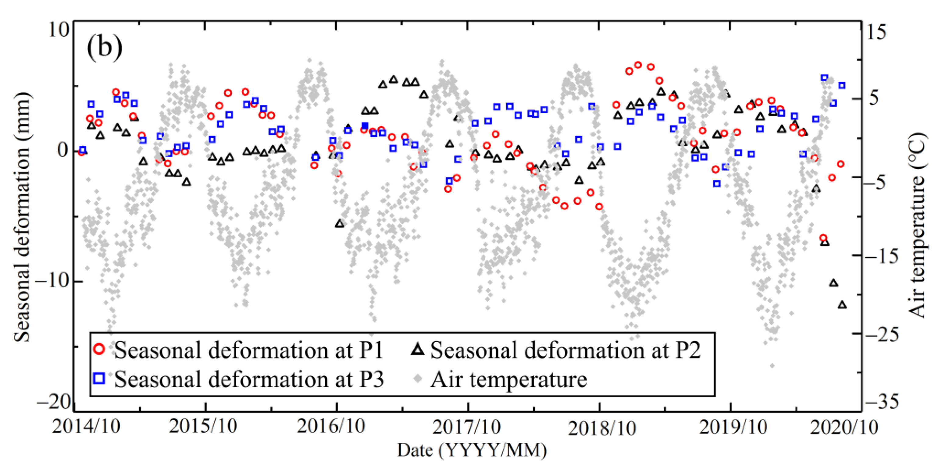
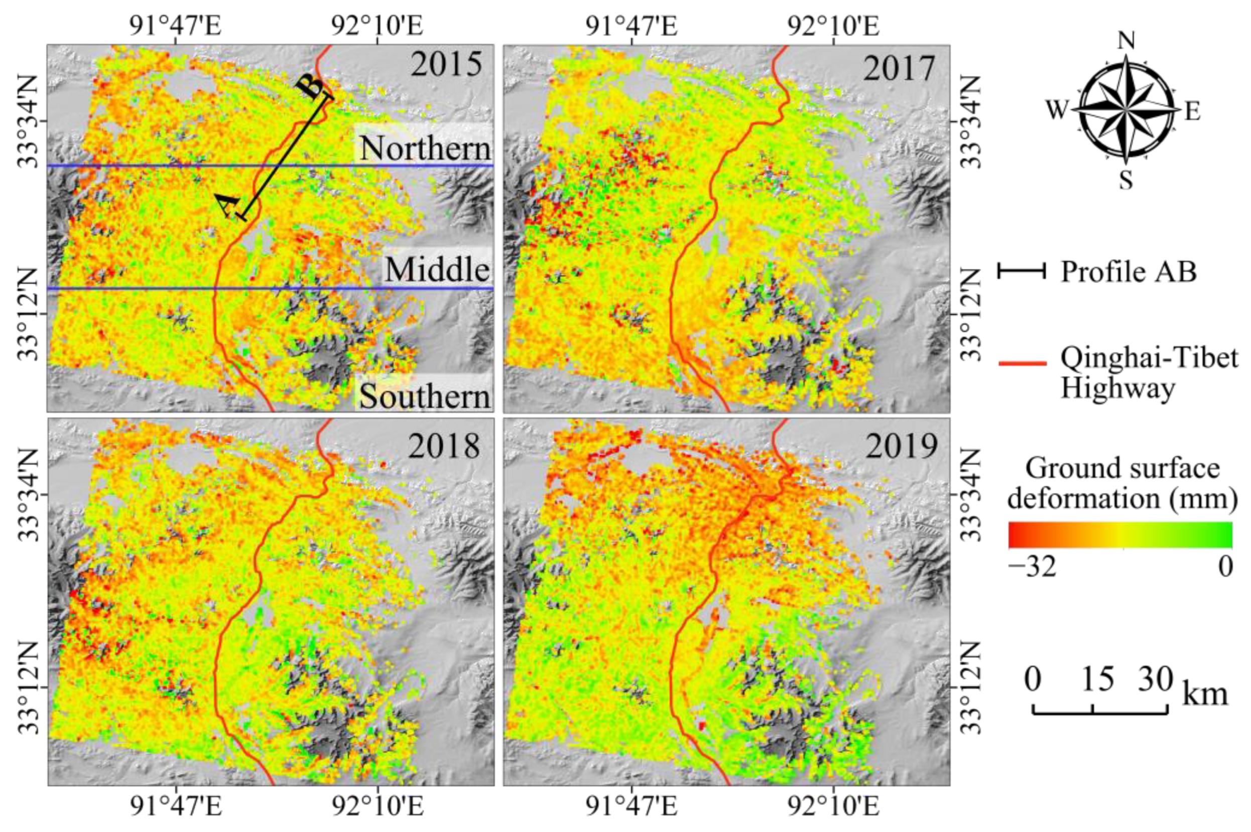
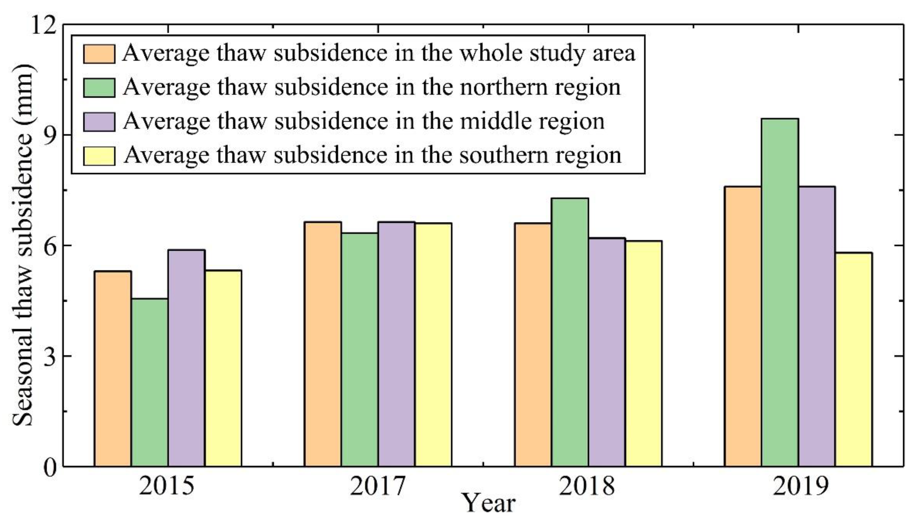
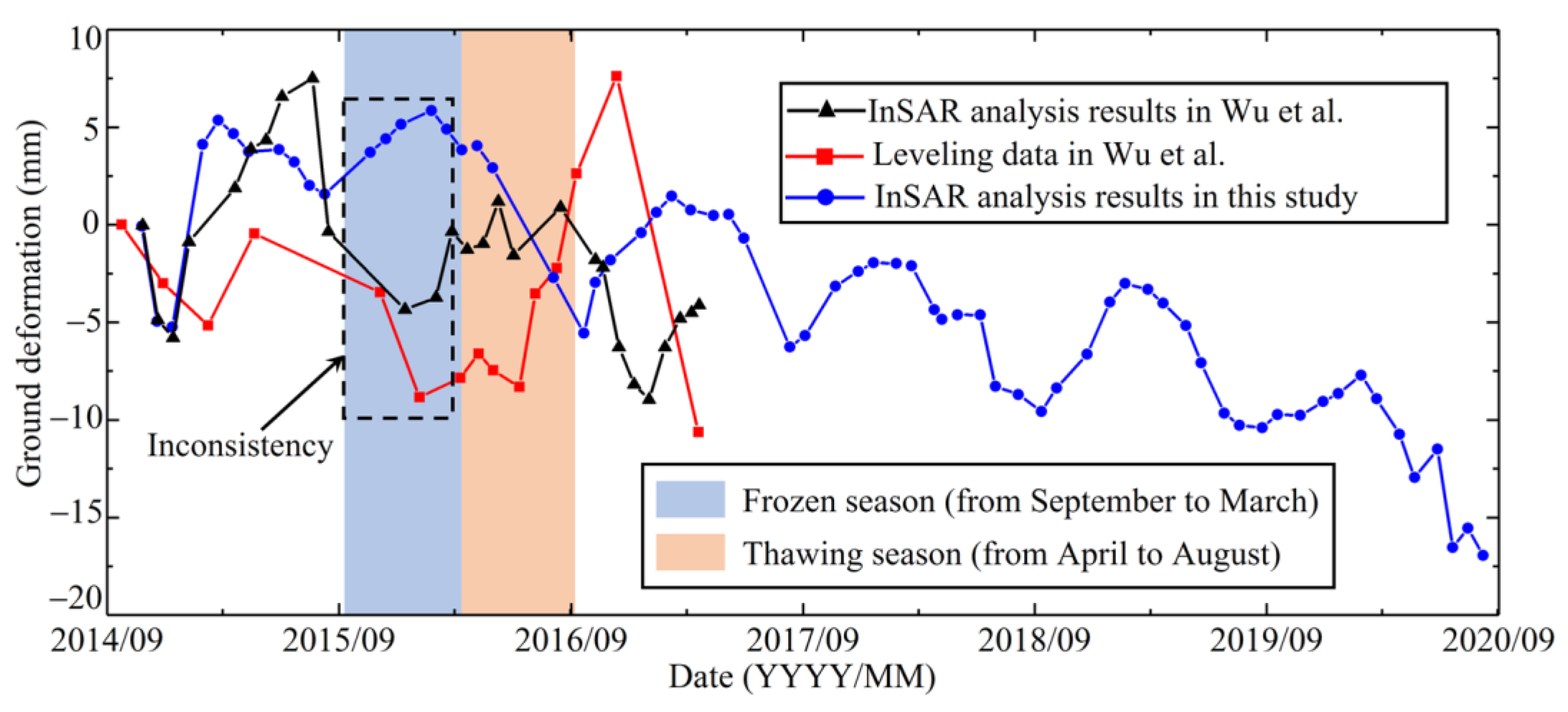
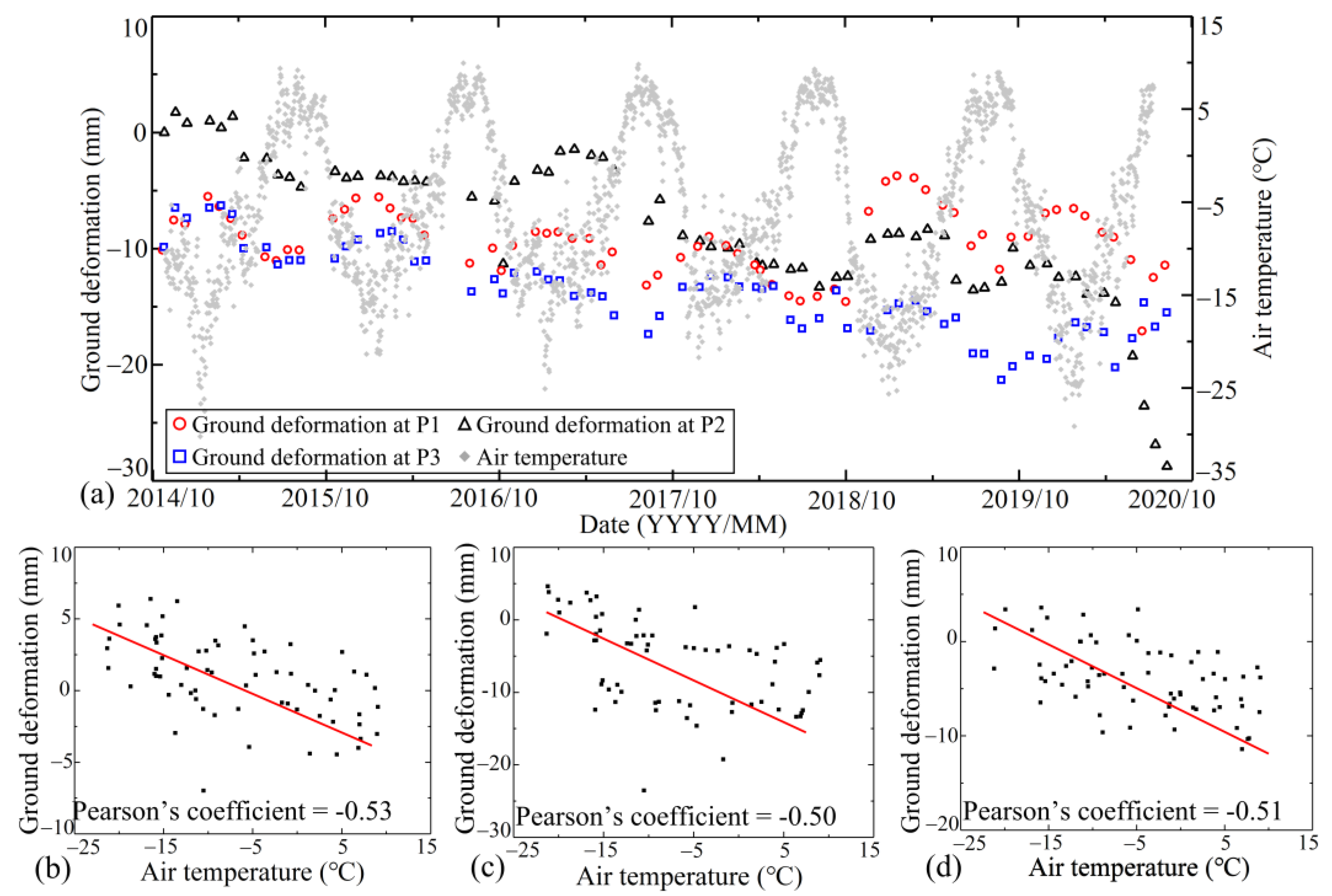
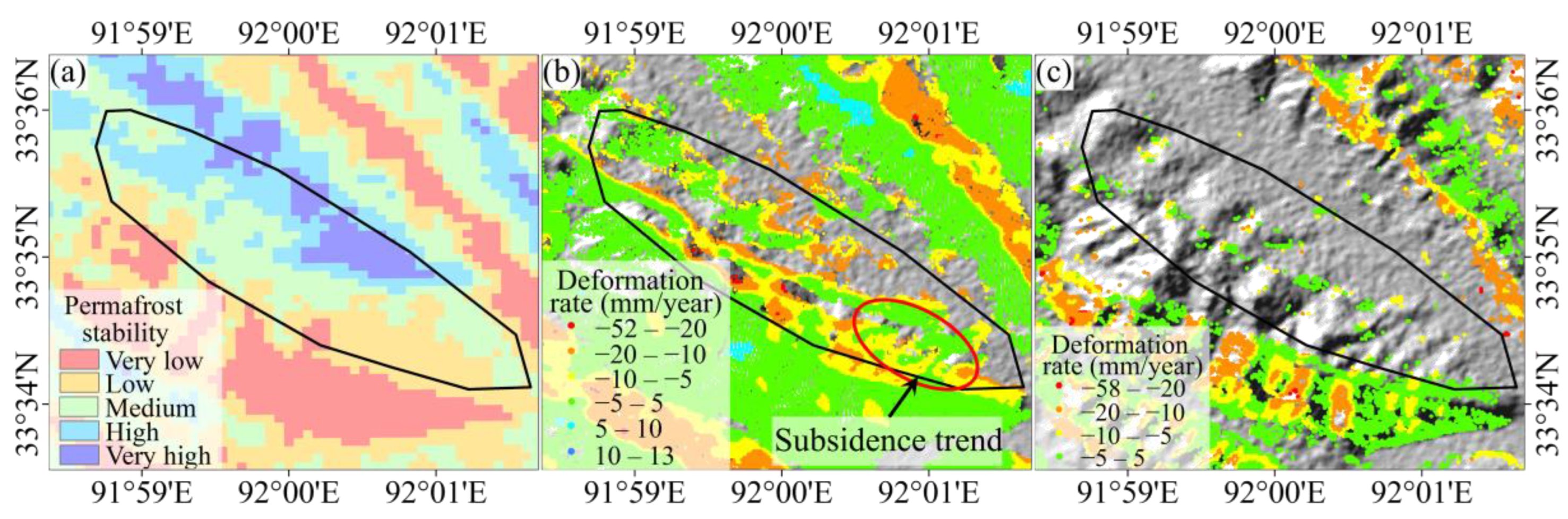
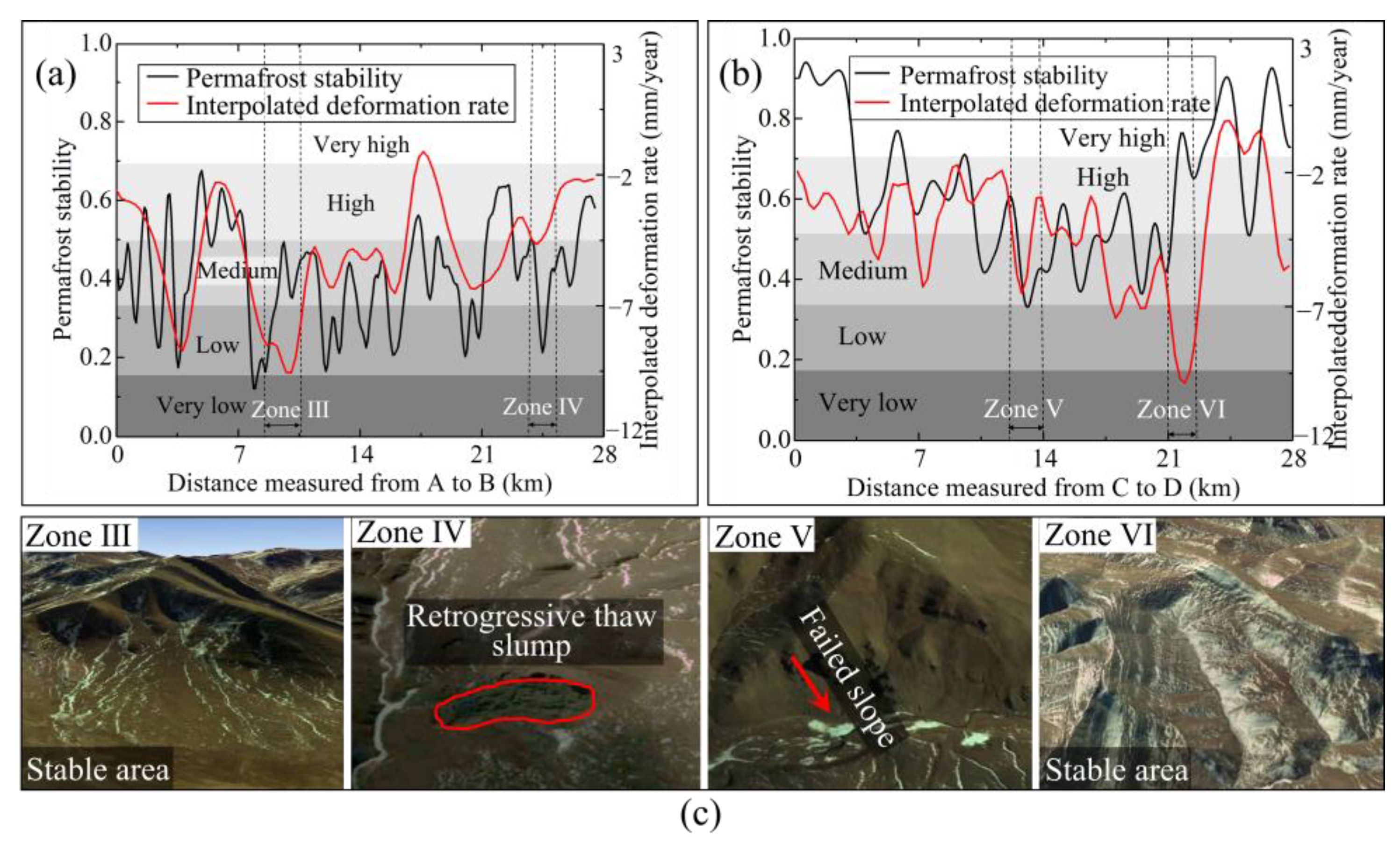
  • The initial InSAR analysis of the ground deformation shows that the maximum ground settlement of the permafrost occurs around the month of August each year, due to the frost heave of the active layer in the frozen season and subsidence in the thawing season, and the magnitude of the ground deformations tends to increase from 2015 to 2019, which might be taken as a sign of the degradation of the permafrost. The initial InSAR analysis also confirms that the seasonal thaw subsidence is strongly affected by the ground elevation topography and vegetation coverage.
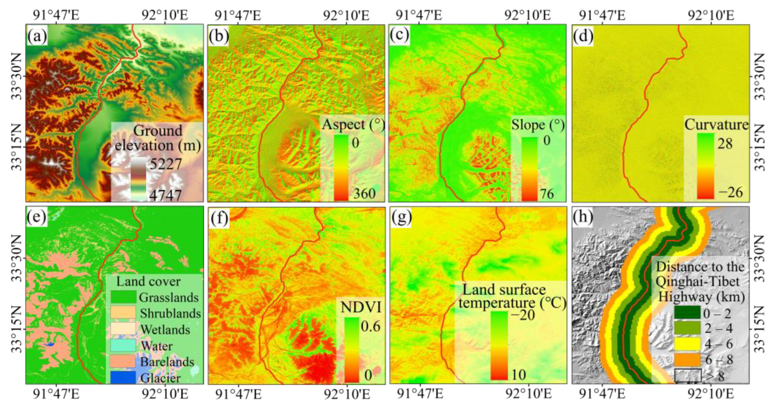
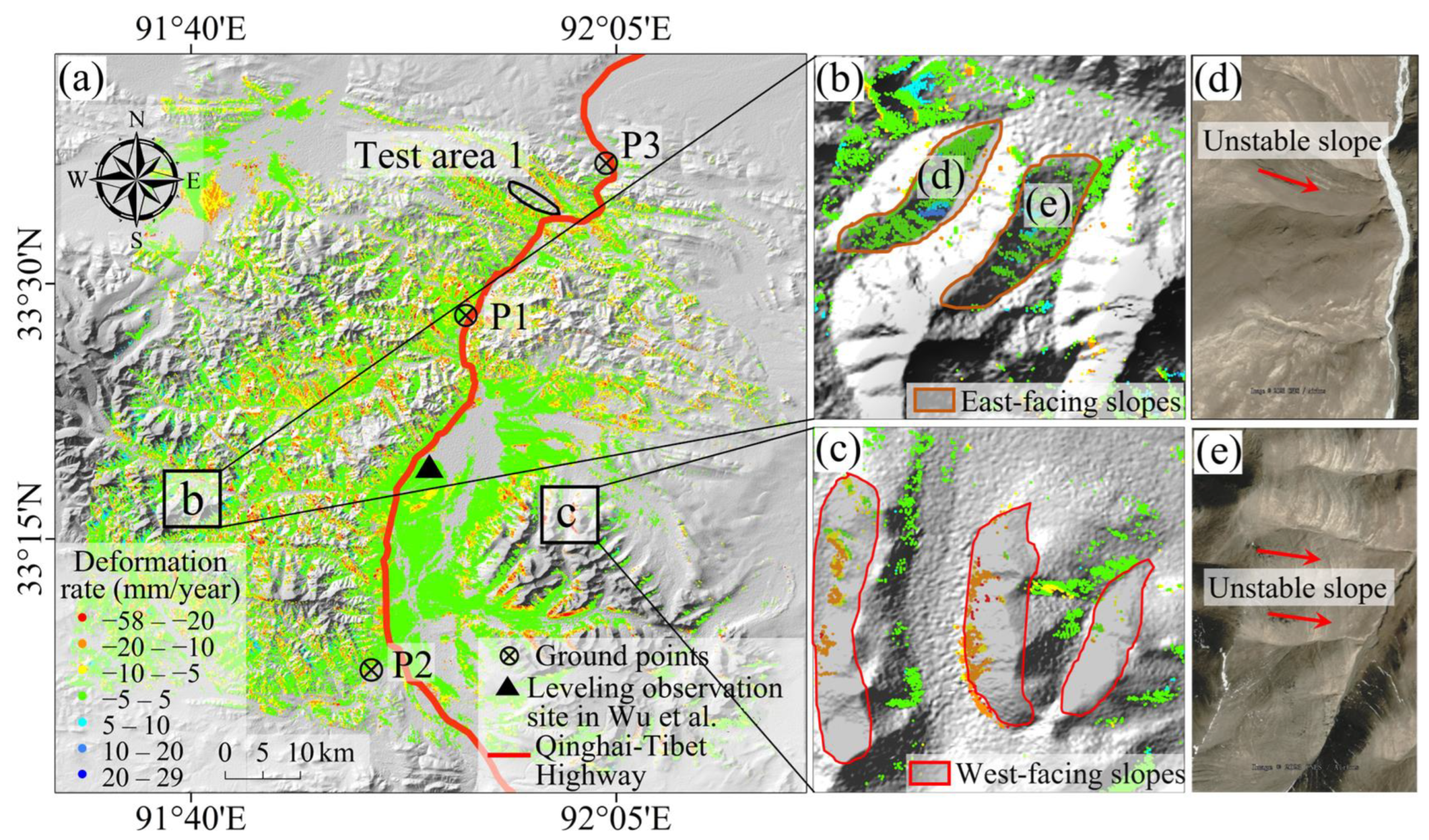
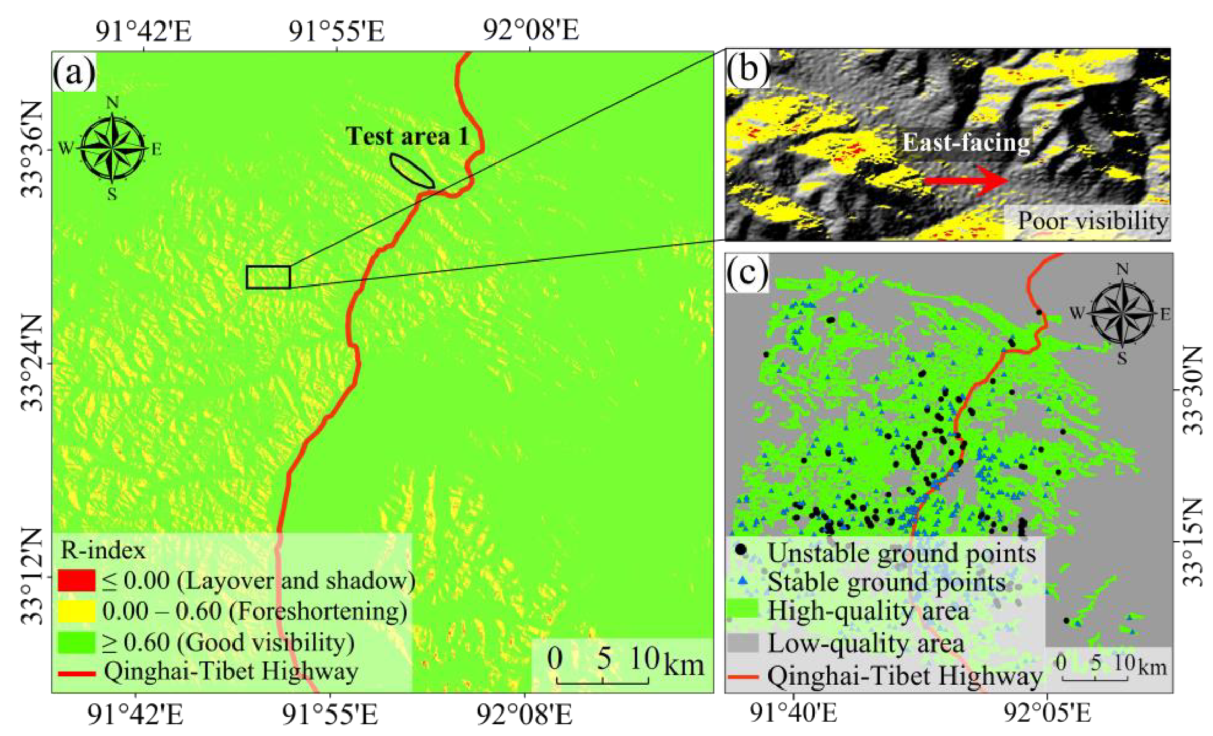
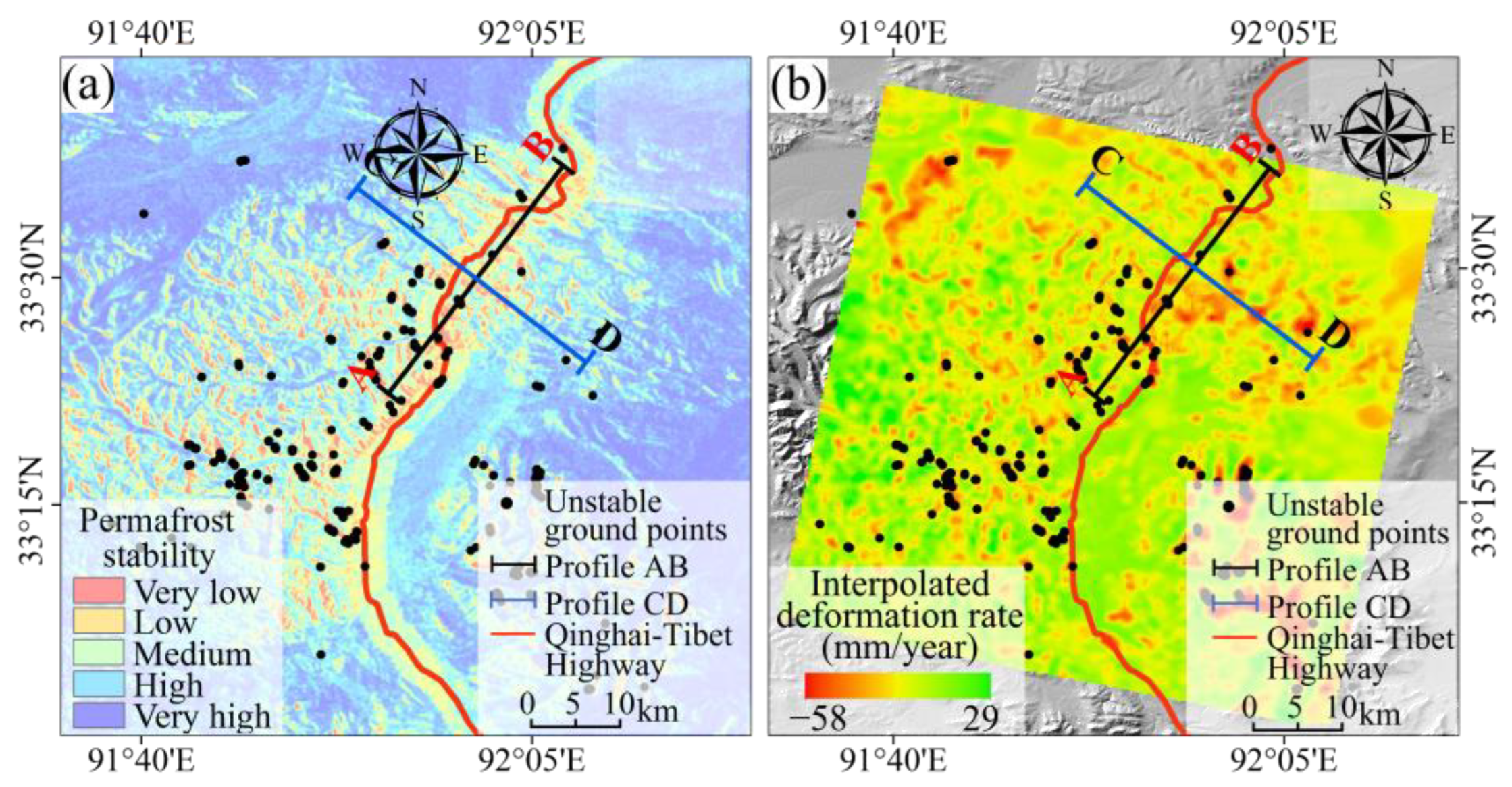
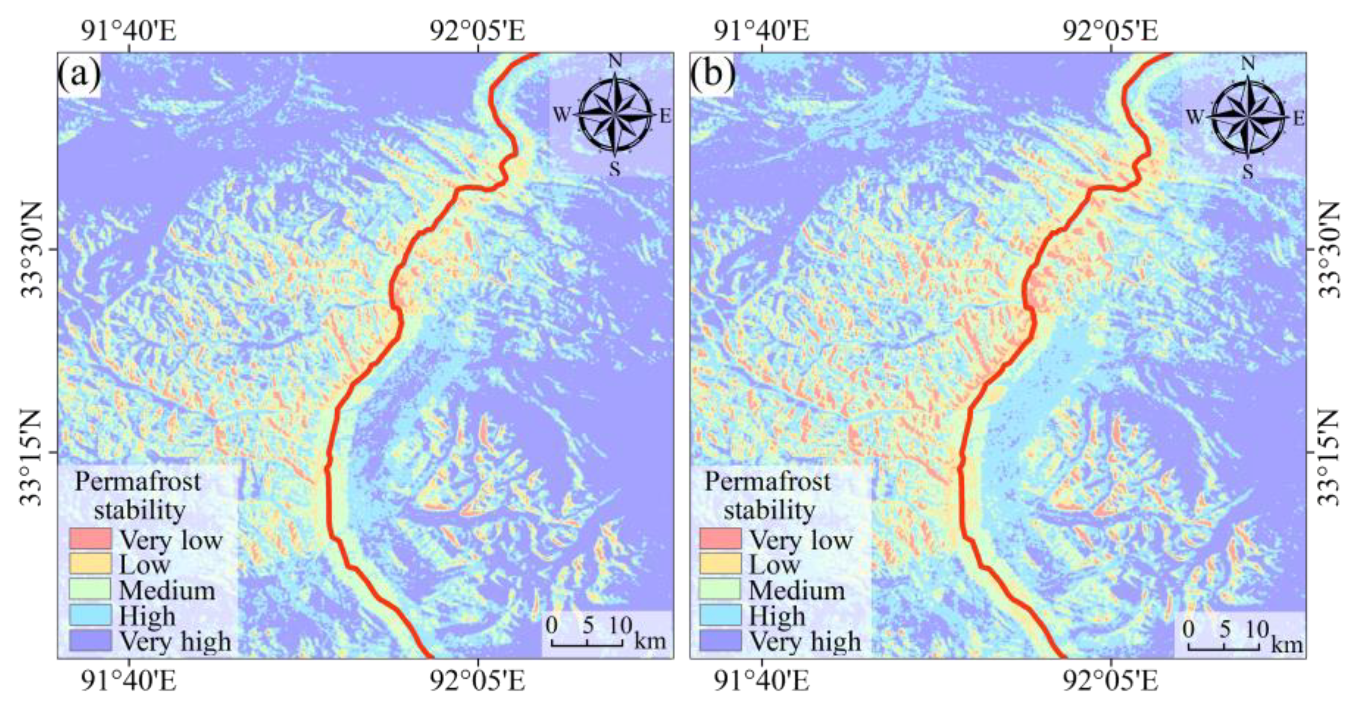
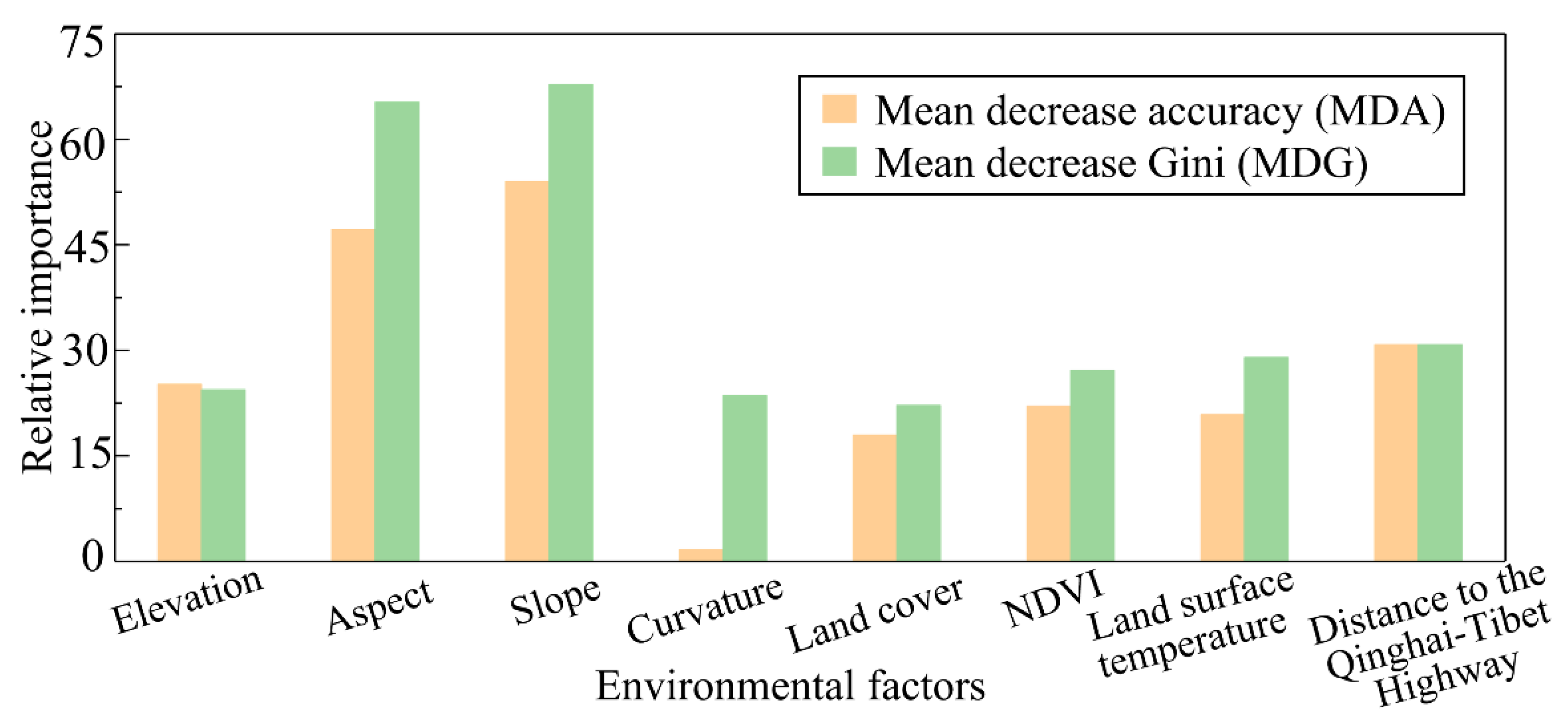
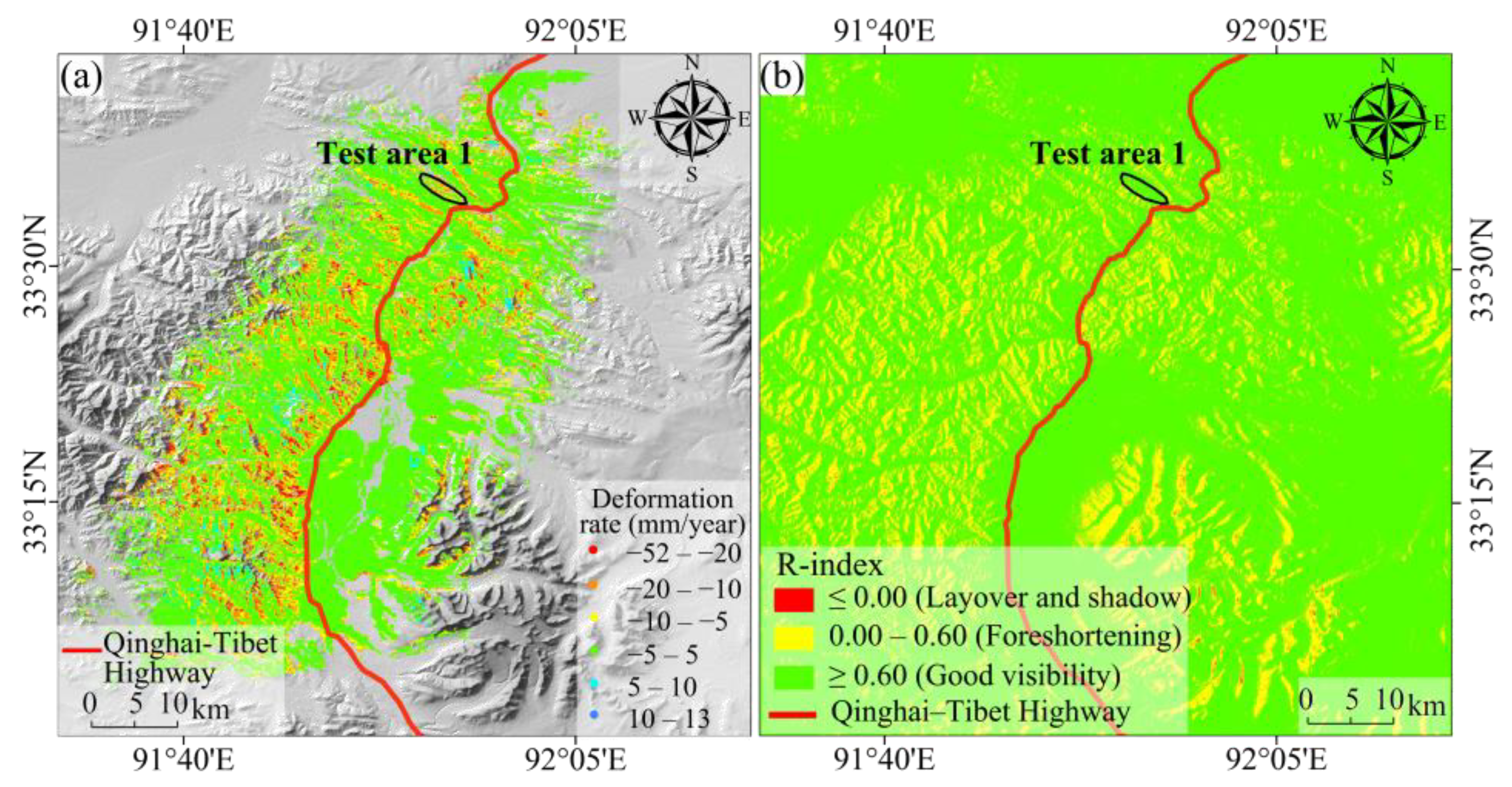
  • According to the analysis of geometric distortion and coherence of the InSAR results, the high-quality areas could be recognized, in which high-quality samples can be readily located based on the threshold values of the ground deformation rate and Google Earth image characteristics. The permafrost stability and associated environmental factors for these high-quality samples can then be extracted for the permafrost stability mapping of the entire study area. The random-forest-based mapping analysis suggests that the permafrost stability (in the study area) is mostly affected by the slope and aspect, whereas the least impact is from the curvature. The factors of ground elevation, land cover, NDVI, land surface temperature, and distance to the highway yield similar importance in the permafrost stability mapping analysis.
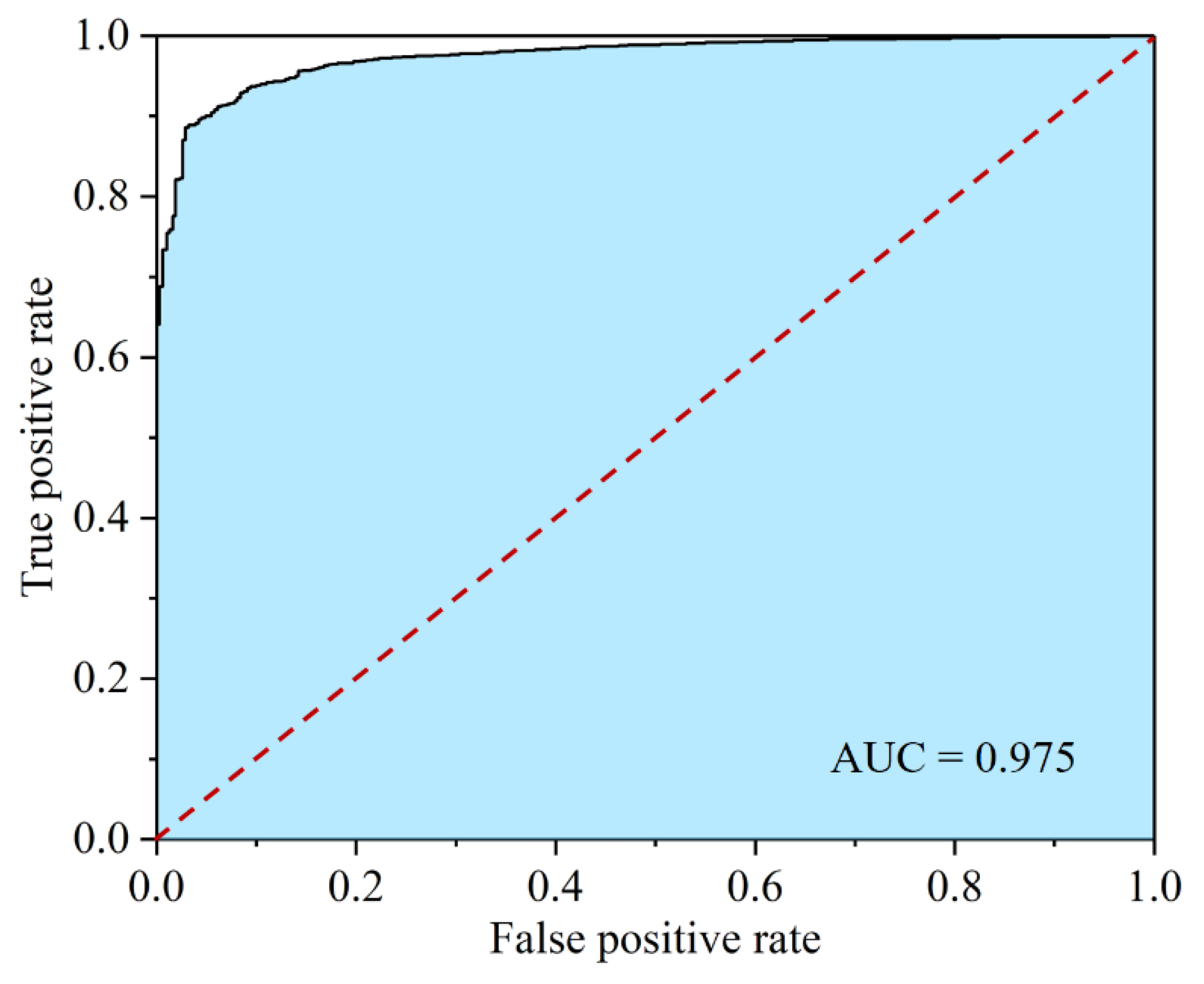
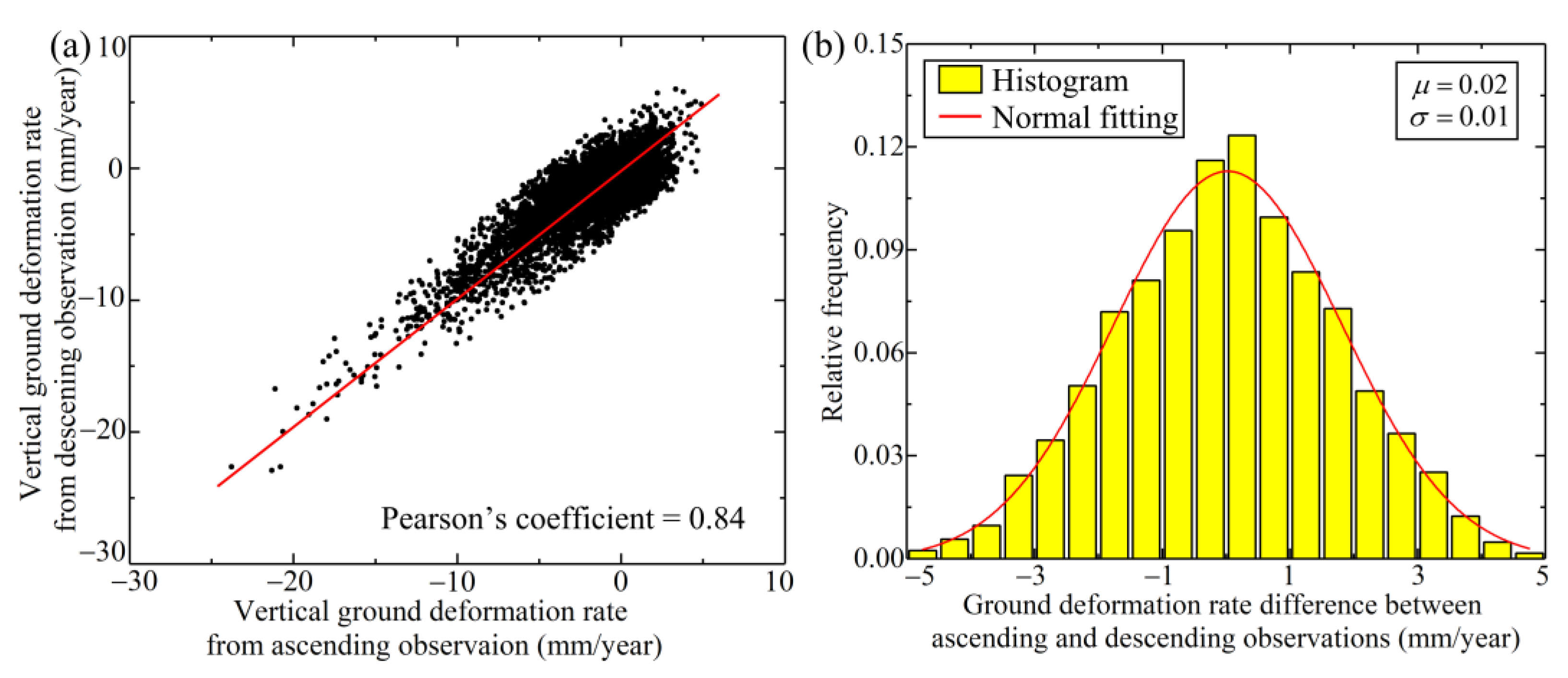
  • The validation analysis of the obtained permafrost stability zonation, which is based on the ROC curve and the unstable ground points in the validation samples, indicates that this integrated method could yield high mapping accuracy in the study area. Through qualitative and quantitative verifications, the ground deformations and the permafrost stability mapping results obtained with the time-series InSAR analysis and the proposed method, respectively, could be validated. Compared with the sole adoption of InSAR analysis, this integrated method is shown to be more effective in permafrost stability mapping of the study area; meanwhile, the issue of data scarcity of InSAR analysis in the low-quality areas could be overcome.
It should be mentioned that although the proposed method has shown to be promising in the permafrost stability mapping of the study area, there is room for improvement. For example, research to further validate the permafrost stability zonation with ground-based measurements is warranted. Moreover, the InSAR analysis in the study is based on the Sentinel-1 C-band SAR images with a 6-day revisiting time, the effectiveness of which is often degraded in mountainous and vegetated areas. Hence, research is also warranted on data fusion methods that could integrate different sources of SAR images.

Author Contributions

Conceptualization, F.Z. and W.G.; methodology, F.Z.; software, T.R.; validation, F.Z., T.R. and J.C.; formal analysis, F.Z. and W.G.; data curation, F.Z.; writing—original draft preparation, F.Z.; writing—review and editing, F.Z. and W.G.; supervision, T.L.; project administration, H.T.; funding acquisition, W.G. and H.T. All authors have read and agreed to the published version of the manuscript.

Funding

This research was funded by the Outstanding Youth Foundation of Hubei Province, China (No. 2022CFA102) and National Natural Science Foundation of China (Grant No. 41977242).

Data Availability Statement

The permafrost classification results are provided by the National Cryosphere Desert Data Center (http://www.ncdc.ac.cn/portal/metadata/16e16d96-482c-4a1a-9345-6f2fa350690e) (accessed on 18 March 2023). The SAR images acquired by Sentinel-1A were downloaded from the European Space Agency (https://scihub.copernicus.eu/dhus/#/home) (accessed on 18 March 2023). The Advanced Land Observing Satellite (ALOS) DEM with a resolution of 12.5 m was downloaded from NASA’s Alaska Satellite Facility Distributed Active Archive Center (https://asf.alaska.edu/) (accessed on 18 March 2023).

Acknowledgments

We appreciate the leveling data and InSAR analysis results provided by Wu et al. [39].

Conflicts of Interest

The authors declare no conflict of interest.

References

  1. Chapin, F.S.; Iii, F.S.C.; Sturm, M.; Serreze, M.C.; McFadden, J.P.; Key, J.R.; Lloyd, A.H.; McGuire, A.D.; Rupp, T.S.; Lynch, A.H.; et al. Role of Land-Surface Changes in Arctic Summer Warming. Science 2005, 310, 657–660. [Google Scholar] [CrossRef]
  2. Hoegh-Guldberg, O.; Jacob, D.; Taylor, M.; Bolaños, T.G.; Bindi, M.; Brown, S.; Camilloni, I.A.; Diedhiou, A.; Djalante, R.; Ebi, K.; et al. The human imperative of stabilizing global climate change at 1.5 °C. Science 2019, 365, eaaw6974. [Google Scholar] [CrossRef]
  3. Fatima, Z.; Ahmed, M.; Hussain, M.; Abbas, G.; Ul-Allah, S.; Ahmad, S.; Ahmed, N.; Ali, M.A.; Sarwar, G.; Haque, E.U.; et al. The fingerprints of climate warming on cereal crops phenology and adaptation options. Sci. Rep. 2020, 10, 1–21. [Google Scholar] [CrossRef]
  4. Nicholas, P.; Raymond, S.B.; Henry, F.D.; Michel, B. Elevation-dependent warming in mountain regions of the world. Nat. Clim. Chang. 2015, 5, 424–443. [Google Scholar]
  5. Biskaborn, B.K.; Smith, S.L.; Noetzli, J.; Matthes, H.; Vieira, G.; Streletskiy, D.A.; Schoeneich, P.; Romanovsky, V.E.; Lewkowicz, A.G.; Abramov, A.; et al. Permafrost is warming at a global scale. Nat. Commun. 2019, 10, 264. [Google Scholar] [CrossRef]
  6. Shan, W.; Zhang, C.; Guo, Y.; Shan, M.; Zeng, X.; Wang, C. Climate Change and surface deformation characteristics in degradation area of permafrost in Lesser Khingan Mountain, China. In Understanding and Reducing Landslide Disaster Risk: Volume 5 Catastrophic Landslides and Frontiers of Landslide Science 5th; Springer: Cham, Switzerland, 2021; pp. 209–219. [Google Scholar]
  7. Luo, J.; Yin, G.; Niu, F.; Lin, Z.; Liu, M. High Spatial Resolution Modeling of Climate Change Impacts on Permafrost Thermal Conditions for the Beiluhe Basin, Qinghai-Tibet Plateau. Remote Sens. 2019, 11, 1294. [Google Scholar] [CrossRef]
  8. Cheng, G.; Zhao, L.; Li, R.; Wu, X.; Sheng, Y. Characteristic changes and impacts of permafrost on Qinghai-Tibet Plateau. Chin. Sci. Bull. 2019, 64, 2783–2795. (In Chinese) [Google Scholar]
  9. Daout, S.; Doin, M.; Peltzer, G.; Socquet, A.; Lasserre, C. Large-scale InSAR monitoring of permafrost freeze-thaw cycles on the Tibetan Plateau. Geophys. Res. Lett. 2017, 44, 901–909. [Google Scholar] [CrossRef]
  10. Huang, L.; Luo, J.; Lin, Z.; Niu, F.; Liu, L. Using deep learning to map retrogressive thaw slumps in the Beiluhe region (Tibetan Plateau) from CubeSat images. Remote Sens. Environ. 2020, 237, 111534. [Google Scholar] [CrossRef]
  11. Lu, P.; Han, J.; Li, Z.; Xu, R.; Li, R.; Hao, T.; Qiao, G. Lake outburst accelerated permafrost degradation on Qinghai-Tibet Plateau. Remote Sens. Environ. 2020, 249, 112011. [Google Scholar] [CrossRef]
  12. Ran, Y.; Jorgenson, M.T.; Li, X.; Jin, H.; Wu, T.; Li, R.; Cheng, G. Biophysical permafrost map indicates ecosystem processes dominate permafrost stability in the Northern Hemisphere. Environ. Res. Lett. 2021, 16, 095010. [Google Scholar] [CrossRef]
  13. Ran, Y.; Li, X.; Cheng, G.; Nan, Z.; Che, J.; Sheng, Y.; Wu, Q.; Jin, H.; Luo, D.; Tang, Z.; et al. Mapping the permafrost stability on the Tibetan Plateau for 2005–2015. Sci. China Earth Sci. 2020, 64, 62–79. [Google Scholar] [CrossRef]
  14. Chen, J.; Wu, T.; Zou, D.; Liu, L.; Wu, X.; Gong, W.; Zhu, X.; Li, R.; Hao, J.; Hu, G.; et al. Magnitudes and patterns of large-scale permafrost ground deformation revealed by Sentinel-1 InSAR on the central Qinghai-Tibet Plateau. Remote Sens. Environ. 2021, 268, 112778. [Google Scholar] [CrossRef]
  15. Park, H.; Kim, Y.; Kimball, J.S. Widespread permafrost vulnerability and soil active layer increases over the high northern latitudes inferred from satellite remote sensing and process model assessments. Remote Sens. Environ. 2016, 175, 349–358. [Google Scholar] [CrossRef]
  16. Vasiliev, A.A.; Drozdov, D.S.; Gravis, A.G.; Malkova, G.V.; Nyland, K.E.; Streletskiy, D.A. Permafrost degradation in the Western Russian Arctic. Environ. Res. Lett. 2020, 15, 045001. [Google Scholar] [CrossRef]
  17. Kovakov, V.P.; Shvetsov, P.F. Problems of integral index stability of ground complex of permafrost. In Proceedings of the 5th International Conference on Permafrost, Trondheim, Norway, 2–5 August 1988; Volume 1, pp. 805–808. [Google Scholar]
  18. Smith, S.L.; Wolfe, S.A.; Riseborough, D.W.; Nixon, F.M. Active-layer characteristics and summer climatic indices, Mackenzie Valley, Northwest Territories, Canada. Permafr. Periglac. Process. 2009, 20, 201–220. [Google Scholar] [CrossRef]
  19. Liu, L.; Schaefer, K.; Gusmeroli, A.; Grosse, G.; Jones, B.M.; Zhang, T.; Parsekian, A.D.; Zebker, H.A. Seasonal thaw settlement at drained thermokarst lake basins, Arctic Alaska. Cryosphere 2014, 8, 815–826. [Google Scholar] [CrossRef]
  20. Wu, Q.; Zhang, T. Changes in active layer thickness over the Qinghai-Tibetan Plateau from 1995 to 2007. J. Geophys. Res. Atmos. 2010, 115, D09107. [Google Scholar] [CrossRef]
  21. Shiklomanov, N.I.; Nelson, F.E. Active-layer mapping at regional scales: A 13-year spatial time series for the Kuparuk region, north-central Alaska. Permafr. Periglac. Process. 2002, 13, 219–230. [Google Scholar] [CrossRef]
  22. Mishra, U.; Drewniak, B.; Jastrow, J.D.; Matamala, R.M.; Vitharana, U. Spatial representation of organic carbon and active-layer thickness of high latitude soils in CMIP5 earth system models. Geoderma 2017, 300, 55–63. [Google Scholar] [CrossRef]
  23. Nitze, I.; Heidler, K.; Barth, S.; Grosse, G. Developing and Testing a Deep Learning Approach for Mapping Retrogressive Thaw Slumps. Remote Sens. 2021, 13, 4294. [Google Scholar] [CrossRef]
  24. Yang, Y.; Rogers, B.M.; Fiske, G.; Watts, J.; Potter, S.; Windholz, T.; Mullen, A.; Nitze, I.; Natali, S.M. Mapping retrogressive thaw slumps using deep neural networks. Remote Sens. Environ. 2023, 288, 113495. [Google Scholar] [CrossRef]
  25. Li, R.; Li, Z.; Han, J.; Lu, P.; Qiao, G.; Meng, X.; Hao, T.; Zhou, F. Monitoring surface deformation of permafrost in Wudaoliang Region, Qinghai–Tibet Plateau with ENVISAT ASAR data. Int. J. Appl. Earth Obs. Geoinf. 2021, 104, 102527. [Google Scholar] [CrossRef]
  26. Wagner, A.M.; Lindsey, N.J.; Dou, S.; Gelvin, A.; Saari, S.; Williams, C.; Ekblaw, I.; Ulrich, C.; Borglin, S.; Morales, A.; et al. Permafrost Degradation and Subsidence Observations during a Controlled Warming Experiment. Sci. Rep. 2018, 8, 10908. [Google Scholar] [CrossRef] [PubMed]
  27. Short, N.; LeBlanc, A.M.; Sladen, W.; Oldenborger, G.; Mathon, V.; Brisco, B. RADARSAT-2 D-InSAR for ground displacement in permafrost terrain, validation from Iqaluit Airport, Baffin Island, Canada. Remote Sens. Environ. 2014, 141, 40–51. [Google Scholar] [CrossRef]
  28. Widhalm, B.; Bartsch, A.; Leibman, M.; Khomutov, A. Active-layer thickness estimation from X-band SAR backscatter intensity. Cryosphere 2017, 11, 483–496. [Google Scholar] [CrossRef]
  29. Wang, L.; Marzahn, P.; Bernier, M.; Ludwig, R. Mapping permafrost landscape features using object-based image classification of multi-temporal SAR images. ISPRS J. Photogramm. Remote Sens. 2018, 141, 10–29. [Google Scholar] [CrossRef]
  30. Anderson, J.E.; Douglas, T.A.; Barbato, R.A.; Saari, S.; Edwards, J.D.; Jones, R.M. Linking vegetation cover and seasonal thaw depths in interior Alaska permafrost terrains using remote sensing. Remote Sens. Environ. 2019, 233, 111363. [Google Scholar] [CrossRef]
  31. Gao, H.; Nie, N.; Zhang, W.; Chen, H. Monitoring the spatial distribution and changes in permafrost with passive microwave remote sensing. ISPRS J. Photogramm. Remote Sens. 2020, 170, 142–155. [Google Scholar] [CrossRef]
  32. Lu, P.; Han, J.; Hao, T.; Li, R.; Qiao, G. Seasonal deformation of permafrost in Wudaoliang basin in Qinghai-Tibet Plateau revealed by StaMPS-InSAR. Mar. Geod. 2019, 43, 248–268. [Google Scholar] [CrossRef]
  33. Colesanti, C.; Wasowski, J. Investigating landslides with space-borne Synthetic Aperture Radar (SAR) interferometry. Eng. Geol. 2006, 88, 173–199. [Google Scholar] [CrossRef]
  34. Ren, T.; Gong, W.; Bowa, V.M.; Tang, H.; Chen, J.; Zhao, F. An Improved R-Index Model for Terrain Visibility Analysis for Landslide Monitoring with InSAR. Remote Sens. 2021, 13, 1938. [Google Scholar] [CrossRef]
  35. Guzzetti, F.; Reichenbach, P.; Cardinali, M.; Galli, M.; Ardizzone, F. Probabilistic landslide hazard assessment at the basin scale. Geomorphology 2005, 72, 272–299. [Google Scholar] [CrossRef]
  36. Gemitzi, A.; Falalakis, G.; Eskioglou, P.; Petalas, C. Evaluating landslide susceptibility using environmental factors, fuzzy membership functions and GIS. Glob. Nest. J. 2011, 13, 28–40. [Google Scholar]
  37. Ciampalini, A.; Raspini, F.; Lagomarsino, D.; Catani, F.; Casagli, N. Landslide susceptibility map refinement using PSInSAR data. Remote Sens. Environ. 2016, 184, 302–315. [Google Scholar] [CrossRef]
  38. Mu, C.; Abbott, B.W.; Norris, A.J.; Mu, M.; Fan, C.; Chen, X.; Jia, L.; Yang, R.; Zhang, T.; Wang, K.; et al. The status and stability of permafrost carbon on the Tibetan Plateau. Earth-Sci. Rev. 2020, 211, 103433. [Google Scholar] [CrossRef]
  39. Wu, Z.; Zhao, L.; Liu, L.; Zhu, R.; Gao, Z.; Qiao, Y.; Xie, M. Surface-deformation monitoring in the permafrost regions over the Tibetan Plateau using Sentinel-1 data. Sci. Cold Arid Reg. 2018, 10, 114–125. [Google Scholar]
  40. Wang, Z.; Yue, G.; Wu, X.; Zhang, W.; Song, X.; Wang, P.; Wu, J. Surface Deformation over Permafrost Environment of the Tanggula Section in the Qinghai-Tibet Plateau Using Active Microwave Spectral Imagines. IOP Conf. Ser. Earth Environ. Sci. 2019, 384, 012211. [Google Scholar] [CrossRef]
  41. Zhao, L.; Zou, D.; Hu, G.; Wu, T.; Du, E.; Liu, G.; Xiao, Y.; Li, R.; Pang, Q.; Qiao, Y.; et al. A synthesis dataset of permafrost thermal state for the Qinghai–Tibet (Xizang) Plateau, China. Earth Syst. Sci. Data 2021, 13, 4207–4218. [Google Scholar] [CrossRef]
  42. Chen, F.; Lin, H.; Zhou, W.; Hong, T.; Wang, G. Surface deformation detected by ALOS PALSAR small baseline SAR interferometry over permafrost environment of Beiluhe section, Tibet Plateau, China. Remote Sens. Environ. 2013, 138, 10–18. [Google Scholar] [CrossRef]
  43. Zhao, R.; Li, Z.W.; Feng, G.C.; Wang, Q.J.; Hu, J. Monitoring surface deformation over permafrost with an improved SBAS-InSAR algorithm: With emphasis on climatic factors modeling. Remote Sens. Environ. 2016, 184, 276–287. [Google Scholar] [CrossRef]
  44. Goldstein, R.M.; Werner, C.L. Radar interferogram filtering for geophysical applications. Geophys. Res. Lett. 1998, 25, 4035–4038. [Google Scholar] [CrossRef]
  45. Bekaert, D.P.S.; Hooper, A.; Wright, T.J. A spatially variable power law tropospheric correction technique for InSAR data. J. Geophys. Res. Solid Earth 2015, 120, 1345–1356. [Google Scholar] [CrossRef]
  46. Garthwaite, M.C.; Wang, H.; Wright, T.J. Broadscale interseismic deformation and fault slip rates in the central Tibetan Plateau observed using InSAR. J. Geophys. Res. Solid Earth 2013, 118, 5071–5083. [Google Scholar] [CrossRef]
  47. Costantini, M. A novel phase unwrapping method based on network programming. IEEE Trans. Geosci. Remote Sens. 1998, 36, 813–821. [Google Scholar] [CrossRef]
  48. Lauknes, T.R.; Zebker, H.A.; Larsen, Y. InSAR Deformation Time Series Using an $L_{1}$-Norm Small-Baseline Approach. IEEE Trans. Geosci. Remote Sens. 2011, 49, 536–546. [Google Scholar] [CrossRef]
  49. Wang, C.; Zhang, Z.; Zhang, H.; Zhang, B.; Tang, Y.; Wu, Q. Active layer thickness retrieval of Qinghai-Tibet permafrost using the TerraSAR-X InSAR technique. IEEE J. Sel. Top. Appl. Earth Observ. Remote Sens. 2018, 11, 4403–4413. [Google Scholar] [CrossRef]
  50. Cigna, F.; Bateson, L.B.; Jordan, C.J.; Dashwood, C. Simulating SAR geometric distortions and predicting Persistent Scatterer densities for ERS-1/2 and ENVISAT C-band SAR and InSAR applications: Nationwide feasibility assessment to monitor the landmass of Great Britain with SAR imagery. Remote Sens. Environ. 2014, 152, 441–466. [Google Scholar] [CrossRef]
  51. Notti, D.; Herrera, G.; Bianchini, S.; Meisina, C.; López-Davalillo, J.C.G.; Zucca, F. A methodology for improving landslide PSI data analysis. Int. J. Remote Sens. 2014, 35, 2186–2214. [Google Scholar] [CrossRef]
  52. Huang, F.; Zhang, J.; Zhou, C.; Wang, Y.; Huang, J.; Zhu, L. A deep learning algorithm using a fully connected sparse autoencoder neural network for landslide susceptibility prediction. Landslides 2019, 17, 217–229. [Google Scholar] [CrossRef]
  53. Azarafza, M.; Azarafza, M.; Akgün, H.; Atkinson, P.M.; Derakhshani, R. Deep learning-based landslide susceptibility mapping. Sci. Rep. 2021, 11, 24112. [Google Scholar] [CrossRef] [PubMed]
  54. Park, S.J.; Lee, C.-W.; Lee, S.; Lee, M.-J. Landslide Susceptibility Mapping and Comparison Using Decision Tree Models: A Case Study of Jumunjin Area, Korea. Remote Sens. 2018, 10, 1545. [Google Scholar] [CrossRef]
  55. Shu, H.; Guo, Z.; Qi, S.; Song, D.; Pourghasemi, H.R.; Ma, J. Integrating Landslide Typology with Weighted Frequency Ratio Model for Landslide Susceptibility Mapping: A Case Study from Lanzhou City of Northwestern China. Remote Sens. 2021, 13, 3623. [Google Scholar] [CrossRef]
  56. Breiman, L. Random forests. Mach. Learn. 2001, 45, 5–32. [Google Scholar] [CrossRef]
  57. Han, Q.; Gui, C.; Xu, J.; Lacidogna, G. A generalized method to predict the compressive strength of high-performance concrete by improved random forest algorithm. Constr. Build. Mater. 2019, 226, 734–742. [Google Scholar] [CrossRef]
  58. Taalab, K.; Cheng, T.; Zhang, Y. Mapping landslide susceptibility and types using Random Forest. Big Earth Data 2018, 2, 159–178. [Google Scholar] [CrossRef]
  59. Li, R.; Zhang, M.; Konstantinov, P.; Pei, W.; Tregubov, O.; Li, G. Permafrost degradation induced thaw settlement susceptibility research and potential risk analysis in the Qinghai-Tibet Plateau. Catena 2022, 214, 106239. [Google Scholar] [CrossRef]
  60. Chen, J.; Wu, Y.; O’Connor, M.; Cardenas, M.B.; Schaefer, K.; Michaelides, R.; Kling, G. Active layer freeze-thaw and water storage dynamics in permafrost environments inferred from InSAR. Remote Sens. Environ. 2020, 248, 112007. [Google Scholar] [CrossRef]
  61. Deluigi, N.; Lambiel, C.; Kanevski, M. Data-driven mapping of the potential mountain permafrost distribution. Sci. Total Environ. 2017, 590, 370–380. [Google Scholar] [CrossRef]
  62. Qin, Y.; Zhang, P.; Liu, W.; Guo, Z.; Xue, S. The application of elevation corrected MERRA2 reanalysis ground surface temperature in a permafrost model on the Qinghai-Tibet Plateau. Cold Reg. Sci. Technol. 2020, 175, 103067. [Google Scholar] [CrossRef]
  63. Beck, I.; Ludwig, R.; Bernier, M.; Lévesque, E.; Boike, J. Assessing Permafrost Degradation and Land Cover Changes (1986-2009) using Remote Sensing Data over Umiujaq, Sub-Arctic Québec. Permafr. Periglac. Process. 2015, 26, 129–141. [Google Scholar] [CrossRef]
  64. Yu, F.; Qi, J.; Yao, X.; Liu, Y. Degradation process of permafrost underneath embankments along Qinghai-Tibet Highway: An engineering view. Cold Reg. Sci. Technol. 2013, 85, 150–156. [Google Scholar] [CrossRef]
  65. Mason, S.J.; Graham, N.E. Areas beneath the relative operating characteristics (ROC) and relative operating levels (ROL) curves: Statistical significance and interpretation. Q. J. R. Meteorol. Soc. 2002, 128, 2145–2166. [Google Scholar] [CrossRef]
  66. Liu, Y.; Yang, H.; Wang, S.; Xu, L.; Peng, J. Monitoring and Stability Analysis of the Deformation in the Woda Landslide Area in Tibet, China by the DS-InSAR Method. Remote Sens. 2022, 14, 532. [Google Scholar] [CrossRef]
  67. Guo, R.; Li, S.; Chen, Y.; Li, X.; Yuan, L. Identification and monitoring landslides in Longitudinal Range-Gorge Region with InSAR fusion integrated visibility analysis. Landslides 2020, 18, 551–568. [Google Scholar] [CrossRef]
  68. Zhang, Z.; Wu, Q. Thermal hazards zonation and permafrost change over the Qinghai–Tibet Plateau. Nat. Hazards 2011, 61, 403–423. [Google Scholar] [CrossRef]
  69. Jin, X.-Y.; Jin, H.-J.; Iwahana, G.; Marchenko, S.S.; Luo, D.-L.; Li, X.-Y.; Liang, S.-H. Impacts of climate-induced permafrost degradation on vegetation: A review. Adv. Clim. Chang. Res. 2020, 12, 29–47. [Google Scholar] [CrossRef]
  70. Zhang, X.; Zhang, H.; Wang, C.; Tang, Y.; Zhang, B.; Wu, F.; Wang, J.; Zhang, Z. Active Layer Thickness Retrieval Over the Qinghai-Tibet Plateau Using Sentinel-1 Multitemporal InSAR Monitored Permafrost Subsidence and Temporal-Spatial Multilayer Soil Moisture Data. IEEE Access 2020, 8, 84336–84351. [Google Scholar] [CrossRef]
  71. Jenks, G.F. The data model concept in statistical mapping. Int. Yearb. Cartogr. 1967, 7, 186–190. [Google Scholar]
  72. Zhao, F.; Gong, W.; Tang, H.; Pudasaini, S.P.; Ren, T.; Cheng, Z. An integrated approach for risk assessment of land subsidence in Xi’an, China using optical and radar satellite images. Eng. Geol. 2023, 314, 106983. [Google Scholar] [CrossRef]
  73. Matheron, G. A Simple Substitute for Conditional Expectation: The Disjunctive Kriging. Adv. Geostat. Min. Ind. 1976, 24, 221–236. [Google Scholar] [CrossRef]
  74. Chen, D.; Chen, H.; Zhang, W.; Cao, C.; Zhu, K.; Yuan, X.; Du, Y. Characteristics of the residual surface deformation of multiple abandoned mined-out areas based on a field investigation and SBAS-InSAR: A case study in Jilin, China. Remote Sens. 2020, 12, 3752. [Google Scholar] [CrossRef]
  75. Yazici, B.V.; Gormus, E.T. Investigating persistent scatterer InSAR (PSInSAR) technique efficiency for landslides mapping: A case study in Artvin dam area, in Turkey. Geocarto Int. 2020, 37, 2293–2311. [Google Scholar] [CrossRef]
  76. Yang, M.; Nelson, F.E.; Shiklomanov, N.I.; Guo, D.; Wan, G. Permafrost degradation and its environmental effects on the Tibetan Plateau: A review of recent research. Earth-Sci. Rev. 2010, 103, 31–44. [Google Scholar] [CrossRef]
  77. Tang, M.; Sun, S.; Zhong, Q.; Wu, S. Energy storage and release of underlying surface and weather change. Plateau Meteorol. 1982, 1, 24–34. [Google Scholar]
  78. Hinzman, L.D.; Goering, D.J.; Kane, D.L. A distributed thermal model for calculating soil temperature profiles and depth of thaw in permafrost regions. J. Geophys. Res. Atmos. 1998, 103, 28975–28991. [Google Scholar] [CrossRef]
  79. Zhang, M.; Wen, Z.; Li, D.; Chou, Y.; Zhou, Z.; Zhou, F.; Lei, B. Impact process and mechanism of summertime rainfall on thermal–moisture regime of active layer in permafrost regions of central Qinghai–Tibet Plateau. Sci. Total Environ. 2021, 796, 148970. [Google Scholar] [CrossRef]
Figure 1. General information of the study area: (a) Permafrost types on the Tibetan plateau; (b) Ground elevation map of the study area.
Remotesensing 15 02294 g001
Figure 2. Principle and implementation procedures of the integrated method for permafrost stability mapping.
Remotesensing 15 02294 g002
Figure 3. Environmental factors extracted in the study area: (a) Ground elevation; (b) Aspect; (c) Slope; (d) Curvature; (e) Land cover; (f) NDVI; (g) Land surface temperature; (h) Distance to the Qinghai–Tibet Highway.
Remotesensing 15 02294 g003
Figure 4. InSAR analysis results of the ground deformation in the study area: (a) Vertical ground deformation rate from October 2014 to August 2020 [39]; (b) Ground deformation rate in east-facing slopes; (c) Ground deformation rate in west-facing slopes; (d,e) Google Earth images for east-facing slopes (Image from © Google Earth 2020).
Remotesensing 15 02294 g004
Figure 5. Fitting analysis of the ground deformation in the period from 2014 to 2020: (a) Fitting analysis between the ground deformation and the time; (b) Correlation analysis between the seasonal deformation and the air temperature (note: the air temperature is from the 2.0 m air temperature dataset from the European Centre for Medium-Range Weather Forecasting—Fifth-Generation Reanalysis (ECMWF ERA5)).
Remotesensing 15 02294 g005aRemotesensing 15 02294 g005b
Figure 6. The maximum ground deformations of the study area occurred during the thawing periods in 2015, 2017, 2018, and 2019.
Remotesensing 15 02294 g006
Figure 7. The average seasonal thaw subsidence of the whole study area and the three regions in 2015, 2017, 2018, and 2019.
Remotesensing 15 02294 g007
Figure 8. The influence of the topography on the seasonal thaw subsidence of the permafrost: (a) Average seasonal thaw subsidence of the study area took place in the period from 2015 to 2019; (b) Relationship between the seasonal thaw subsidence and the ground elevation along profile AB; (c) Variations in the seasonal thaw subsidence and the ground elevation with the distance measured from A to B along profile AB; (d) A detailed survey of the topography (Zone I is located in a river valley; Zone II is located on a north-facing slope).
Remotesensing 15 02294 g008
Figure 9. The influence of the vegetation coverage on the seasonal thaw subsidence of the permafrost: (a) Vegetation coverage in the study area; (b) Relationship between the seasonal thaw subsidence and the NDVI along profile AB; (c) Variations in the seasonal thaw subsidence and the NDVI with the distance measured from A to B along profile AB.
Remotesensing 15 02294 g009
Figure 10. Screening analysis of the InSAR analysis results of ground deformation in the study area: (a) Geometric distortion analysis results; (b) A detailed survey of the geometric distortions on an east-facing slope; (c) Zonation of the high-quality and low-quality areas.
Remotesensing 15 02294 g010
Figure 11. Permafrost stability mapping in the study area: (a) Results of the permafrost stability mapping with the trained random forest model; (b) Ground deformation rate obtained by the Kriging interpolation of initial InSAR analysis (Note: Profiles AB and CD are delineated to compare the two permafrost stability results).
Remotesensing 15 02294 g011
Figure 12. Validation of the trained random forest model using the ROC curve.
Remotesensing 15 02294 g012
Figure 13. Permafrost stability mapping using different classification schemes: (a) Equal intervals; (b) Standard deviations.
Remotesensing 15 02294 g013
Figure 14. The relative importance of the environmental factors to the permafrost stability.
Remotesensing 15 02294 g014
Figure 15. Verifications of the time-series InSAR analysis results with the leveling data and InSAR analysis results obtained by Wu et al. [39] (Reprinted with permission from ref. [39]. Copyright 2018 Copyright Sciences in Cold and Arid Regions).
Remotesensing 15 02294 g015
Figure 16. Relationships between the ground deformation and the air temperature: (a) Relationships between the ground deformation and the air temperature at points P1, P2, and P3; (bd) Correlations between the ground deformation and the air temperature at points P1, P2, and P3.
Remotesensing 15 02294 g016
Figure 17. InSAR analysis results in the study area obtained from the ascending Sentinel-1 SAR images: (a) Vertical ground deformation rate from October 2014 to August 2020; (b) Geometric distortion analysis results.
Remotesensing 15 02294 g017
Figure 18. Comparison of the ground deformation rate obtained from ascending and descending SAR images: (a) Correlation analysis of the vertical ground deformation rates obtained from ascending and descending SAR images; (b) Distribution of the ground deformation rate differences between ascending and descending SAR images.
Remotesensing 15 02294 g018
Figure 19. Comparisons between the permafrost stability mapping results in Test Area 1 obtained with the proposed method and the ground deformations obtained from the ascending SAR images: (a) Permafrost stability mapping results obtained with the proposed method; (b) Vertical ground deformation rates obtained from the ascending SAR images; (c) Vertical ground deformation rates obtained from the descending SAR images.
Remotesensing 15 02294 g019
Figure 20. Comparisons between the proposed method and the sole application of InSAR analysis: (a) Permafrost stability zonation obtained by the proposed method versus the ground deformation rate obtained by the Kriging interpolation of initial InSAR analysis along profile AB; (b) Permafrost stability zonation obtained by the integrated method versus the ground deformation rate obtained by the Kriging interpolation of initial InSAR analysis along profile CD; (c) A detailed survey of the permafrost stability in Zones III, IV, V, and VI with the Google Earth images (note: Zones III and VI are located in areas with medium and high permafrost stability and Zones IV and V are located in areas with low permafrost stability. Image from © Google Earth 2019).
Remotesensing 15 02294 g020
Disclaimer/Publisher’s Note: The statements, opinions and data contained in all publications are solely those of the individual author(s) and contributor(s) and not of MDPI and/or the editor(s). MDPI and/or the editor(s) disclaim responsibility for any injury to people or property resulting from any ideas, methods, instructions or products referred to in the content.

