

A Twenty-Year Assessment of Spatiotemporal Variation of Surface Temperature in the Yangtze River Delta, China

Abstract
:1. Introduction
2. Date and Methods
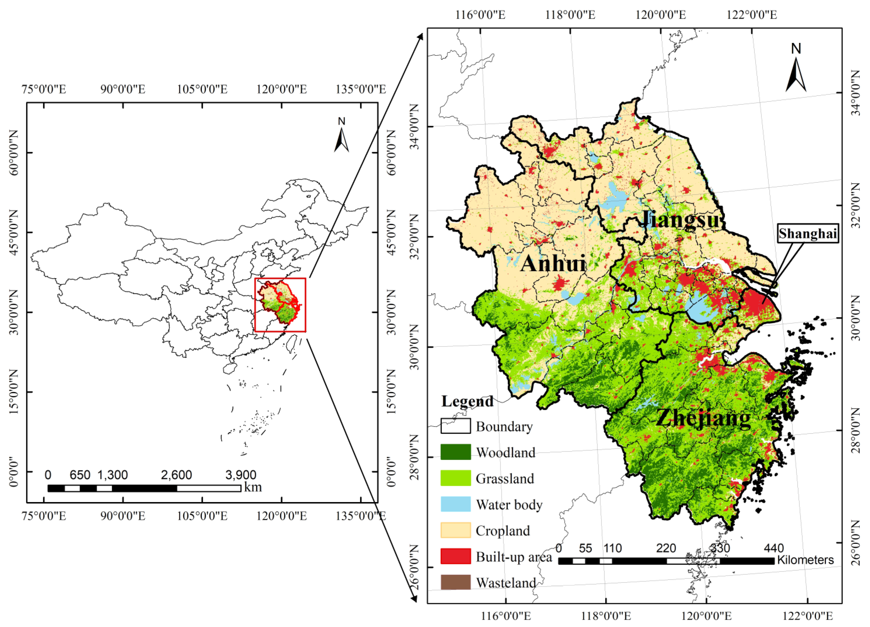
2.1. Study Area
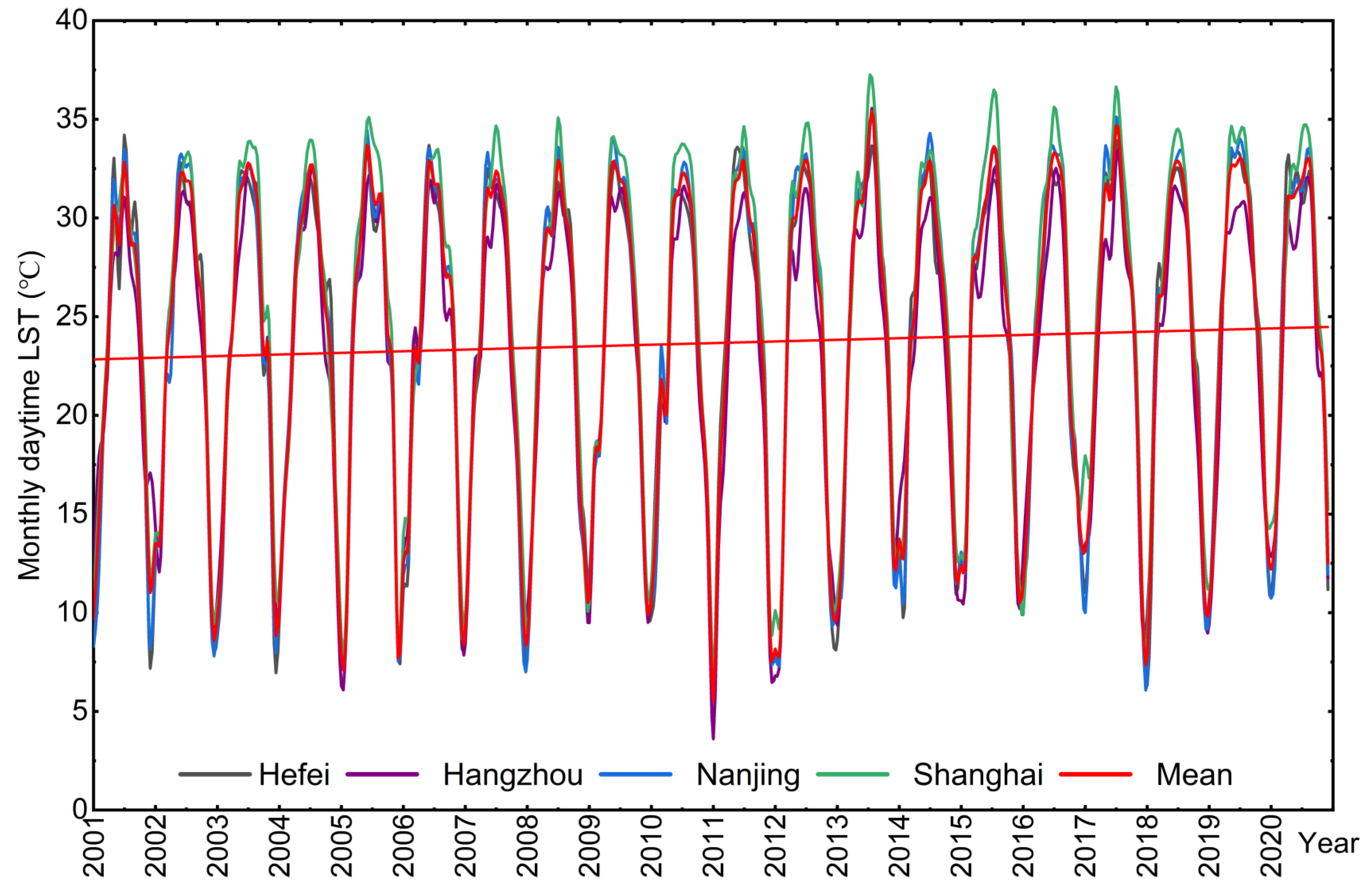
2.2. LST, NDVI and LCT Data
2.3. Theil–Sen Median Trend Analysis and Mann–Kendall Test
2.4. BFAST Algorithm
- (1)
- An additive model is used to decompose the original time series into a trend component, a seasonal component, and a residual component. The algorithm is formulated as follows:where is the observed value at time , is the trend component, is the seasonal component, and is the residual component.
- (2)
- A segmented linear fit is used to fit the trend component . For each trend segment after defining , the linear model algorithm is as follows:
- (3)
- For the seasonal component , the harmonic model is fitted due to the obvious periodic variation of LST. For each trend segment , after defining , the harmonic model can be expressed as:
2.5. Landscape Pattern Analysis
3. Results and Discussion
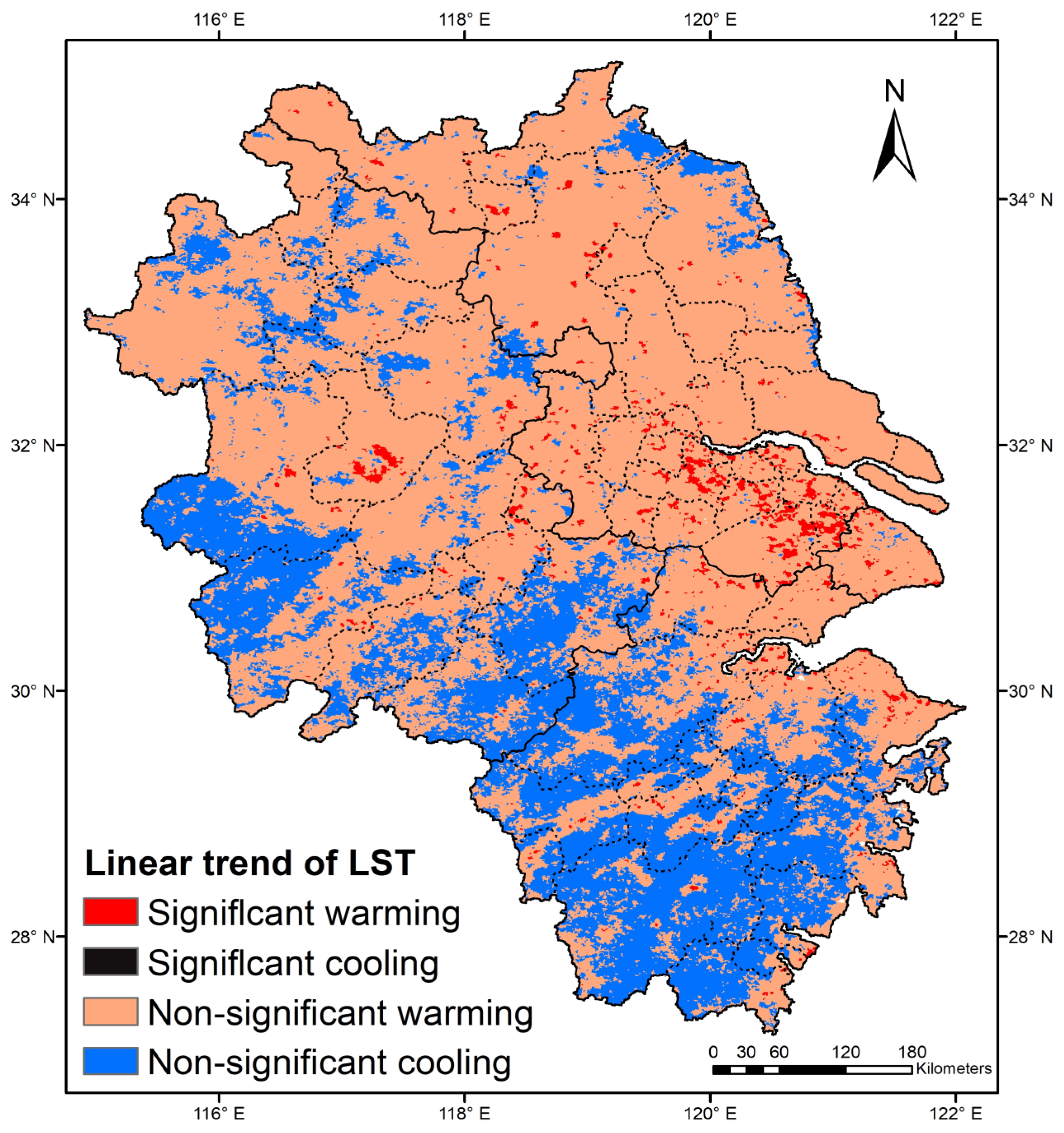
3.1. Linear LST Trends Based on Theil–Sen Median Trend Analysis and the Mann–Kendall
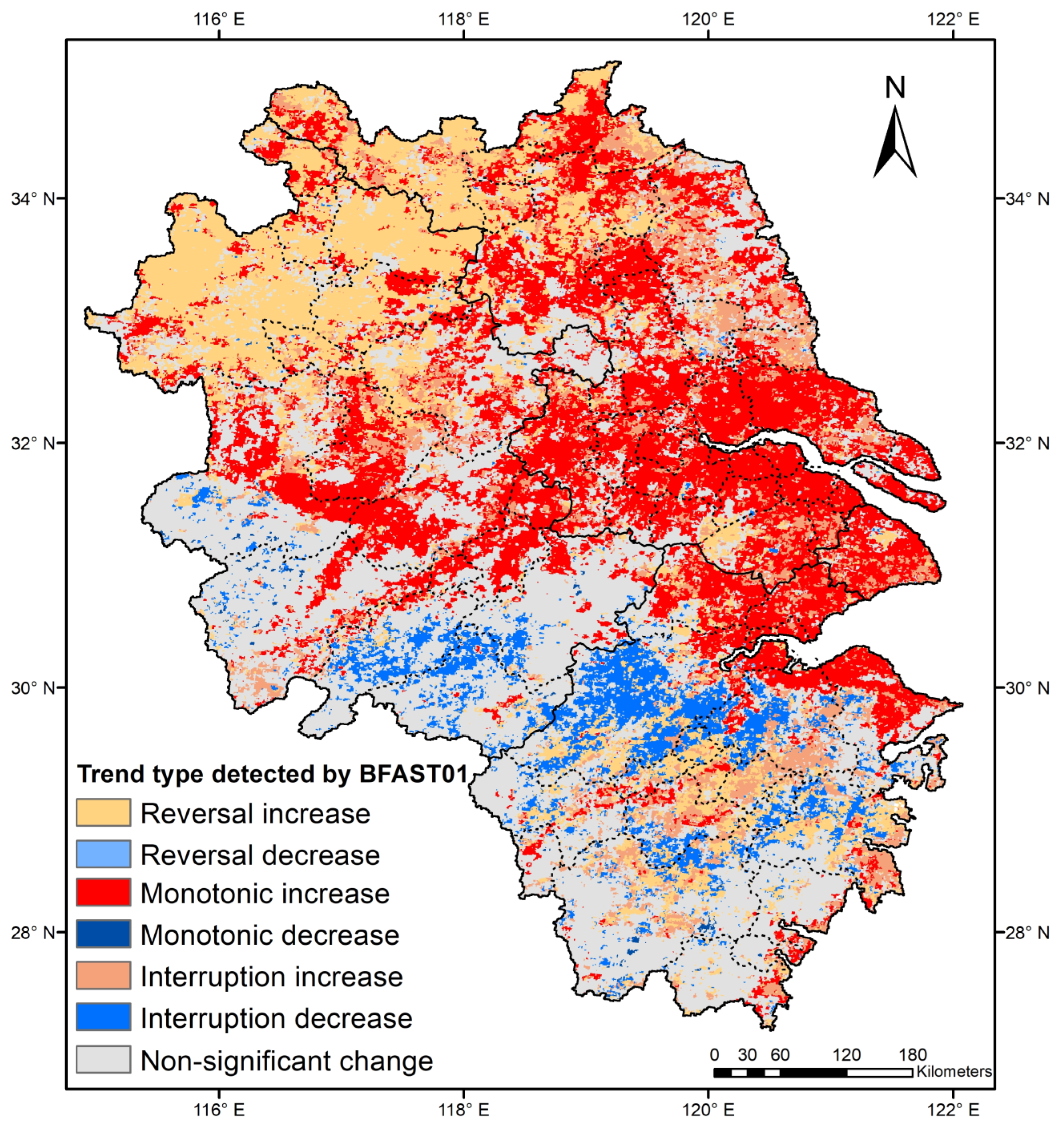
3.2. LST Variations Based on BFAST01 Decomposition
3.2.1. LST Trends Based on BFAST01 Decomposition
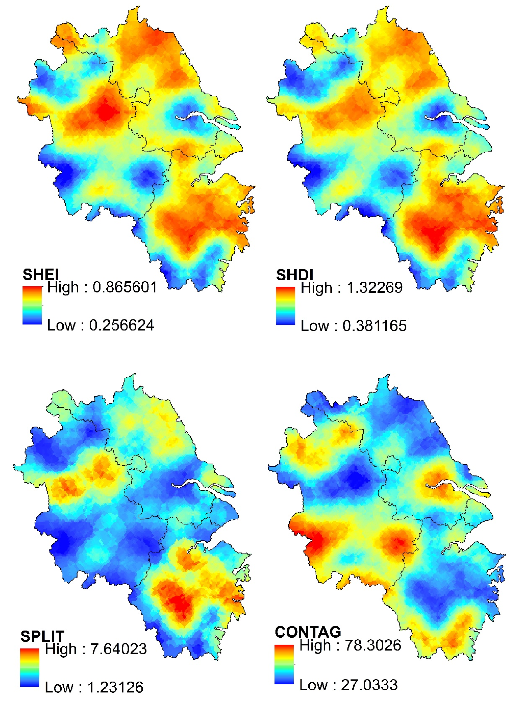
3.2.2. Landscape Pattern Analysis
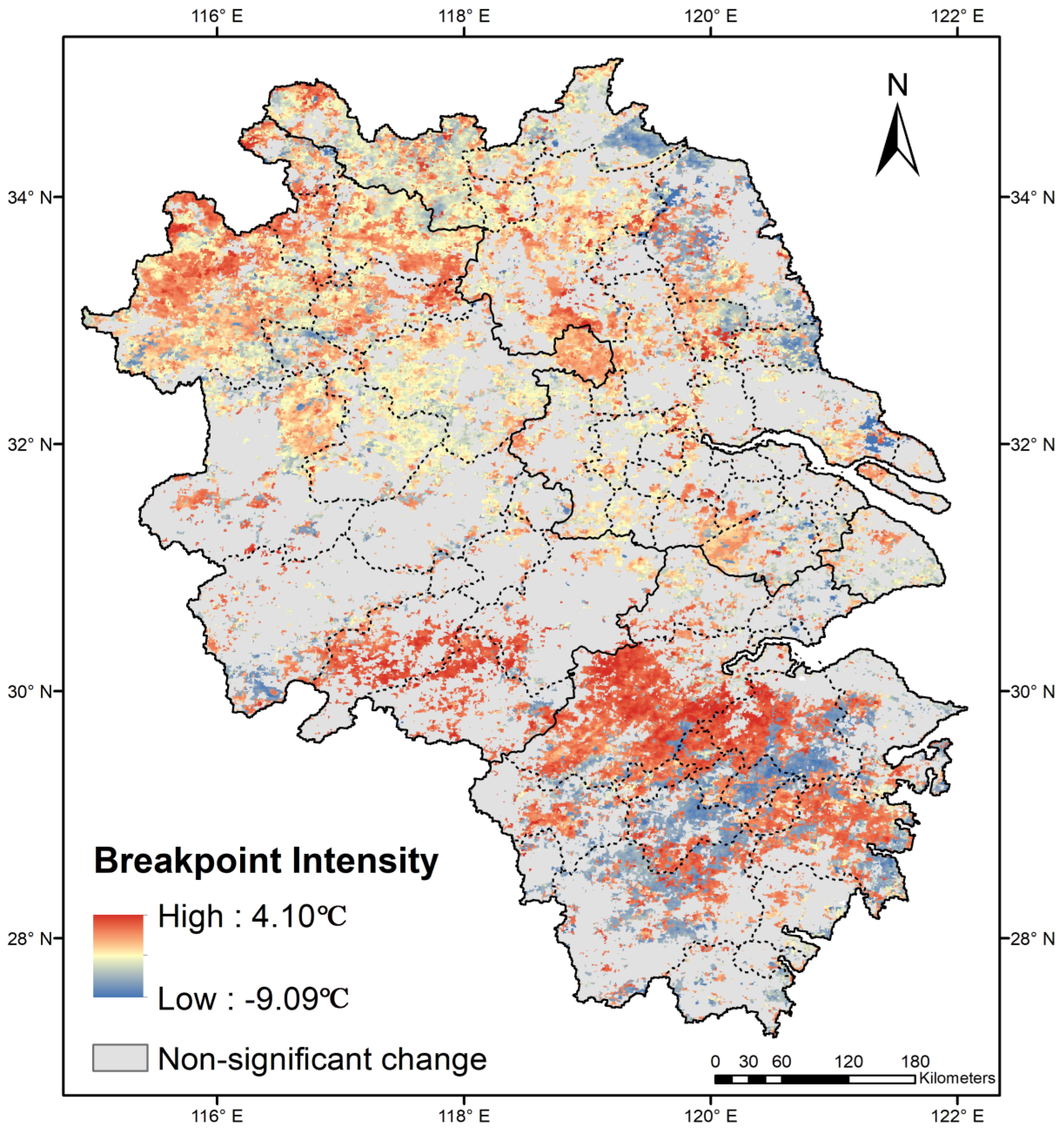
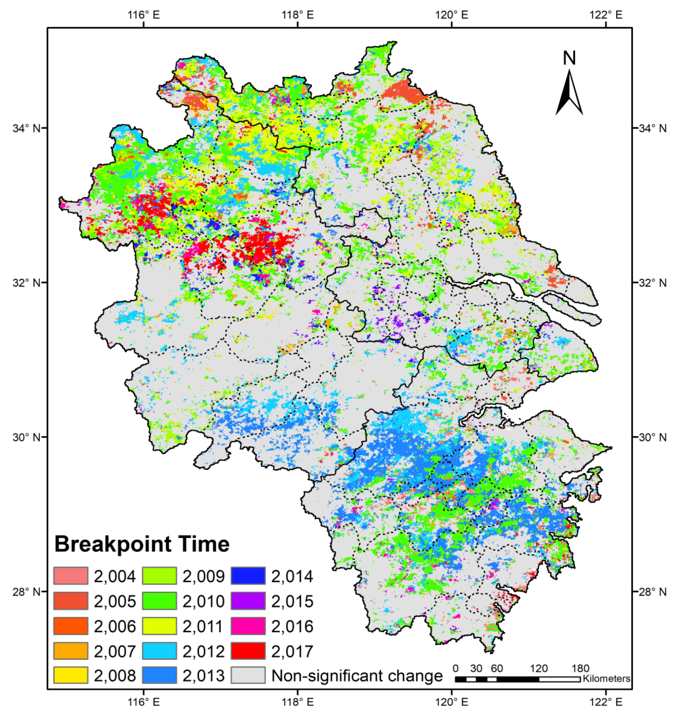
3.2.3. Breakpoint Strength, Occurrence Times and Spatial Distribution
3.3. Attributions of LST Trends
3.3.1. NDVI, LCT and the LST Breakpoints
3.3.2. NDVI, LCT and the Type Derived by BFAST01 Trend Decomposition
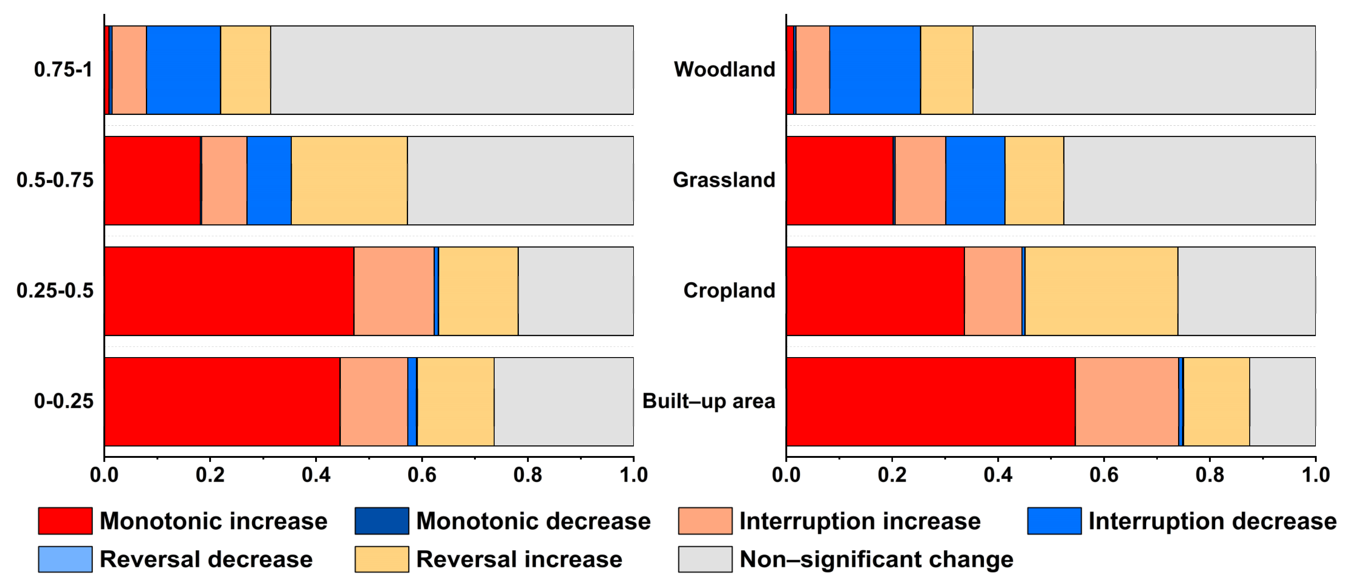
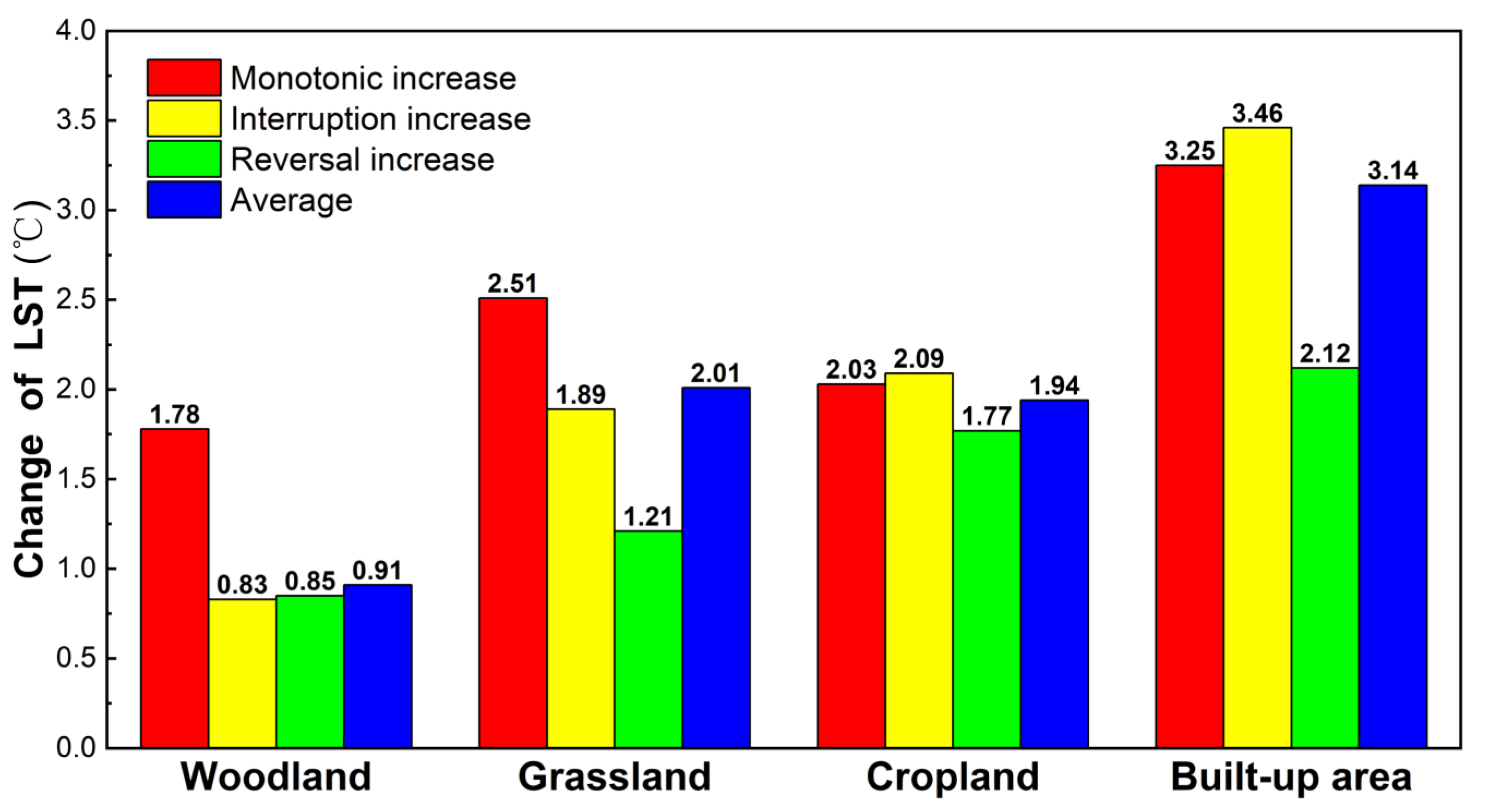
3.4. The Inconsistent Warming of Different LCTs
4. Conclusions
- (1)
- The linear rate of change of LST in the YRD ranged from −0.019 °C/month to 0.046 °C/month, with a more pronounced warming trend in the north and near urban agglomerations. However, within the warming trend, it is mainly composed of monotonic increases (27.3%), reversal increases (19.3%) and interruption increases (10.64%). The landscape index shows a strong aggregation of the type derived by BFAST01 trend decomposition, but low connectivity and high spatial heterogeneity. Monotonic increases and non-significant trends are more dominant.
- (2)
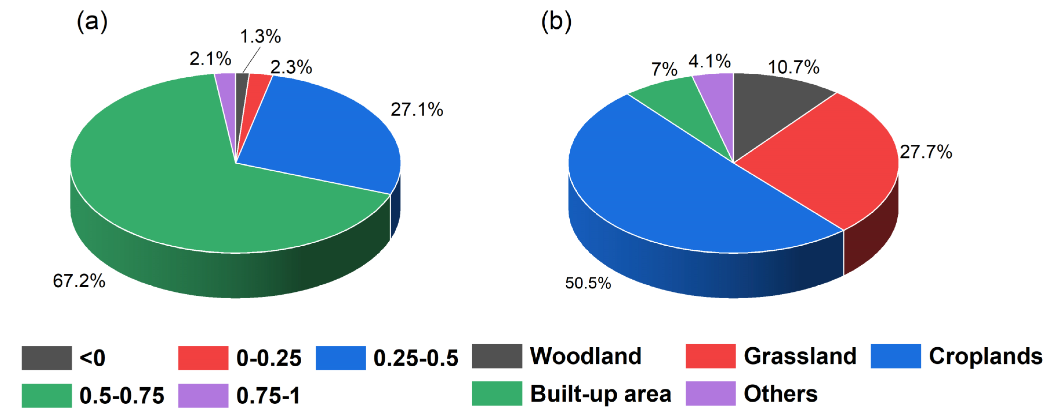
- The breakpoints are widely distributed in the YRD but are more concentrated in the southern and northern regions. The intensity of the breakpoints is mostly within 2 °C, with reference to the linear trend rate of change, which typically takes 3.62–8.77 years to offset an abrupt change. The breakpoints are highly concentrated in the period 2010–2013, suggesting stronger external disturbances in this period. Breakpoints occurred more frequently over cropland and the NDVI range of 0.5–0.7, indicating more disturbances over these areas.
- (3)
- The types of LST trends varied considerably for different NDVI levels and LCTs. In general, the proportion of non-significant trends generally increases gradually as the NDVI level increases. Within a global warming background, this suggests a suppressive effect of vegetation on LST warming. The warming in the built-up area is significantly higher than in the other LCTS, with monotonic warming and interrupted warming contributing more to warming.
Author Contributions
Funding
Data Availability Statement
Conflicts of Interest
References
- Diffenbaugh, N.S.; Burke, M. Global warming has increased global economic inequality. Proc. Natl. Acad. Sci. USA 2019, 116, 9808–9813. [Google Scholar] [CrossRef] [PubMed]
- King, A.D.; Karoly, D.J.; Henley, B.J. Australian climate extremes at 1.5 degrees C and 2 degrees C of global warming. Nat. Clim. Chang. 2017, 12, 114031. [Google Scholar] [CrossRef]
- Hansen, J.; Ruedy, R.; Sato, M.; Lo, K. Global Surface Temperature Change. Rev. Geophys. 2010, 48. [Google Scholar] [CrossRef]
- Li, Z.L.; Tang, B.H.; Wu, H.; Ren, H.Z.; Yan, G.J.; Wan, Z.M.; Trigo, I.F.; Sobrino, J.A. Satellite-derived land surface temperature: Current status and perspectives. Remote Sens. Environ. 2013, 131, 14–37. [Google Scholar] [CrossRef]
- Liu, Z.; Zhan, W.; Bechtel, B.; Voogt, J.; Lai, J.; Chakraborty, T.; Wang, Z.-H.; Li, M.; Huang, F.; Lee, X. Surface warming in global cities is substantially more rapid than in rural background areas. Commun. Earth Environ. 2022, 3, 219. [Google Scholar] [CrossRef]
- Zhan, W.; Chen, Y.; Zhou, J.; Wang, J.; Liu, W.; Voogt, J.; Zhu, X.; Quan, J.; Li, J. Disaggregation of remotely sensed land surface temperature: Literature survey, taxonomy, issues, and caveats. Remote Sens. Environ. 2013, 131, 119–139. [Google Scholar] [CrossRef]
- Aguilar-Lome, J.; Espinoza-Villar, R.; Espinoza, J.-C.; Rojas-Acuña, J.; Willems, B.L.; Leyva-Molina, W.-M. Elevation-dependent warming of land surface temperatures in the Andes assessed using MODIS LST time series (2000–2017). Int. J. Appl. Earth Obs. Geoinf. 2019, 77, 119–128. [Google Scholar] [CrossRef]
- Zhou, D.; Xiao, J.; Frolking, S.; Liu, S.; Zhang, L.; Cui, Y.; Zhou, G. Croplands intensify regional and global warming according to satellite observations. Remote Sens. Environ. 2021, 264, 112585. [Google Scholar] [CrossRef]
- Camuffo, D.; Bertolin, C. The earliest temperature observations in the world: The Medici Network (1654–1670). Clim. Chang. 2012, 111, 335–363. [Google Scholar] [CrossRef]
- Stahl, K.; Moore, R.D.; Floyer, J.A.; Asplin, M.G.; McKendry, I.G. Comparison of approaches for spatial interpolation of daily air temperature in a large region with complex topography and highly variable station density. Agric. For. Meteorol. 2006, 139, 224–236. [Google Scholar] [CrossRef]
- Eleftheriou, D.; Kiachidis, K.; Kalmintzis, G.; Kalea, A.; Bantasis, C.; Koumadoraki, P.; Spathara, M.E.; Tsolaki, A.; Tzampazidou, M.I.; Gemitzi, A. Determination of annual and seasonal daytime and nighttime trends of MODIS LST over Greece—Climate change implications. Sci. Total Environ. 2018, 616, 937–947. [Google Scholar] [CrossRef]
- Laraby, K.G.; Schott, J.R. Uncertainty estimation method and Landsat 7 global validation for the Landsat surface temperature product. Remote Sens. Environ. 2018, 216, 472–481. [Google Scholar] [CrossRef]
- Malakar, N.K.; Hulley, G.C.; Hook, S.J.; Laraby, K.; Cook, M.; Schott, J.R. An Operational Land Surface Temperature Product for Landsat Thermal Data: Methodology and Validation. IEEE Trans. Geosci. Remote Sens. 2018, 56, 5717–5735. [Google Scholar] [CrossRef]
- Ding, Y.; Zhang, S.; Zhao, L.; Li, Z.; Kang, S. Global warming weakening the inherent stability of glaciers and permafrost. Sci. Bull. 2019, 64, 245–253. [Google Scholar] [CrossRef]
- Du, Q.; Zhang, M.; Wang, S.; Che, C.; Ma, R.; Ma, Z. Changes in air temperature over China in response to the recent global warming hiatus. J. Geogr. Sci. 2019, 29, 496–516. [Google Scholar] [CrossRef]
- Ji, F.; Wu, Z.; Huang, J.; Chassignet, E.P. Evolution of land surface air temperature trend. Nat. Clim. Chang. 2014, 4, 462–466. [Google Scholar] [CrossRef]
- Croitoru, A.-E.; Holobaca, I.-H.; Lazar, C.; Moldovan, F.; Imbroane, A. Air temperature trend and the impact on winter wheat phenology in Romania. Clim. Chang. 2012, 111, 393–410. [Google Scholar] [CrossRef]
- Sonali, P.; Nagesh Kumar, D. Review of trend detection methods and their application to detect temperature changes in India. J. Hydrol. 2013, 476, 212–227. [Google Scholar] [CrossRef]
- Li, Y.; Yao, N.; Chau, H.W. Influences of removing linear and nonlinear trends from climatic variables on temporal variations of annual reference crop evapotranspiration in Xinjiang, China. Sci. Total Environ. 2017, 592, 680–692. [Google Scholar] [CrossRef]
- Wu, Z.; Huang, N.E.; Long, S.R.; Peng, C.-K. On the trend, detrending, and variability of nonlinear and nonstationary time series. Proc. Natl. Acad. Sci. USA 2007, 104, 14889–14894. [Google Scholar] [CrossRef]
- Panwar, M.; Agarwal, A.; Devadas, V. Analyzing land surface temperature trends using non-parametric approach: A case of Delhi, India. Urban Clim. 2018, 24, 19–25. [Google Scholar] [CrossRef]
- Yu, Y.; Duan, S.-B.; Li, Z.-L.; Chang, S.; Xing, Z.; Leng, P.; Gao, M. Interannual Spatiotemporal Variations of Land Surface Temperature in China From 2003 to 2018. IEEE J. Sel. Top. Appl. Earth Obs. Remote Sens. 2021, 14, 1783–1795. [Google Scholar] [CrossRef]
- Fang, S.; Mao, K.; Xia, X.; Wang, P.; Shi, J.; Bateni, S.M.; Xu, T.; Cao, M.; Heggy, E.; Qin, Z. Dataset of daily near-surface air temperature in China from 1979 to 2018. Earth Syst. Sci. Data 2022, 14, 1413–1432. [Google Scholar] [CrossRef]
- Zhao, P.; Jones, P.; Cao, L.; Yan, Z.; Zha, S.; Zhu, Y.; Yu, Y.; Tang, G. Trend of Surface Air Temperature in Eastern China and Associated Large-Scale Climate Variability over the Last 100 Years. J. Clim. 2014, 27, 4693–4703. [Google Scholar] [CrossRef]
- El Kenawy, A.; López-Moreno, J.I.; Vicente-Serrano, S.M. Trend and variability of surface air temperature in northeastern Spain (1920–2006): Linkage to atmospheric circulation. Atmos. Res. 2012, 106, 159–180. [Google Scholar] [CrossRef]
- Kennedy, R.E.; Yang, Z.; Cohen, W.B. Detecting trends in forest disturbance and recovery using yearly Landsat time series: 1. LandTrendr—Temporal segmentation algorithms. Remote Sens. Environ. 2010, 114, 2897–2910. [Google Scholar] [CrossRef]
- Jamali, S.; Jönsson, P.; Eklundh, L.; Ardö, J.; Seaquist, J. Detecting changes in vegetation trends using time series segmentation. Remote Sens. Environ. 2015, 156, 182–195. [Google Scholar] [CrossRef]
- Verbesselt, J.; Hyndman, R.; Newnham, G.; Culvenor, D. Detecting trend and seasonal changes in satellite image time series. Remote Sens. Environ. 2010, 114, 106–115. [Google Scholar] [CrossRef]
- Jacquin, A.; Sheeren, D.; Lacombe, J.-P. Vegetation cover degradation assessment in Madagascar savanna based on trend analysis of MODIS NDVI time series. Int. J. Appl. Earth Obs. Geoinf. 2010, 12, S3–S10. [Google Scholar] [CrossRef]
- Bassingthwaighte, J.B.; Raymond, G.M. Evaluating rescaled range analysis for time series. Ann. Biomed. Eng. 1994, 22, 432–444. [Google Scholar] [CrossRef]
- Iida, T.; Saitoh, S.-I. Temporal and spatial variability of chlorophyll concentrations in the Bering Sea using empirical orthogonal function (EOF) analysis of remote sensing data. Deep. Sea Res. Part II Top. Stud. Oceanogr. 2007, 54, 2657–2671. [Google Scholar] [CrossRef]
- Hawinkel, P.; Swinnen, E.; Lhermitte, S.; Verbist, B.; Van Orshoven, J.; Muys, B. A time series processing tool to extract climate-driven interannual vegetation dynamics using Ensemble Empirical Mode Decomposition (EEMD). Remote Sens. Environ. 2015, 169, 375–389. [Google Scholar] [CrossRef]
- Fang, X.; Zhu, Q.; Ren, L.; Chen, H.; Wang, K.; Peng, C. Large-scale detection of vegetation dynamics and their potential drivers using MODIS images and BFAST: A case study in Quebec, Canada. Remote Sens. Environ. 2018, 206, 391–402. [Google Scholar] [CrossRef]
- Shen, X.; An, R.; Feng, L.; Ye, N.; Zhu, L.; Li, M. Vegetation changes in the Three-River Headwaters Region of the Tibetan Plateau of China. Ecol. Indic. 2018, 93, 804–812. [Google Scholar] [CrossRef]
- Xie, M.; Liao, J.B.; Wang, T.J.; Zhu, K.G.; Zhuang, B.L.; Han, Y.; Li, M.M.; Li, S. Modeling of the anthropogenic heat flux and its effect on regional meteorology and air quality over the Yangtze River Delta region, China. Atmos. Chem. Phys. 2016, 16, 6071–6089. [Google Scholar] [CrossRef]
- Yang, X.C.; Leung, L.R.; Zhao, N.Z.; Zhao, C.; Qian, Y.; Hu, K.J.; Liu, X.P.; Chen, B.D. Contribution of urbanization to the increase of extreme heat events in an urban agglomeration in east China. Geophys. Res. Lett. 2017, 44, 6940–6950. [Google Scholar] [CrossRef]
- Yao, R.; Hu, Y.Q.; Sun, P.; Bian, Y.J.; Liu, R.L.; Zhang, S.L. Effects of urbanization on heat waves based on the wet-bulb temperature in the Yangtze River Delta urban agglomeration, China. Urban Clim. 2022, 41, 101067. [Google Scholar] [CrossRef]
- Qian, L.X.; Cui, H.S.; Jie, C. Impacts of land use and cover change on land surface temperature in the Zhujiang Delta. Pedosphere 2006, 16, 681–689. [Google Scholar] [CrossRef]
- Song, Z.J.; Li, R.H.; Qiu, R.Y.; Liu, S.Y.; Tan, C.; Li, Q.P.; Ge, W.; Han, X.J.; Tang, X.G.; Shi, W.Y.; et al. Global Land Surface Temperature Influenced by Vegetation Cover and PM2.5 from 2001 to 2016. Remote Sens. 2018, 10, 2034. [Google Scholar] [CrossRef]
- Yang, B.; Yang, X.C.; Leung, L.R.; Zhong, S.Y.; Qian, Y.; Zhao, C.; Chen, F.; Zhang, Y.C.; Qi, J.G. Modeling the Impacts of Urbanization on Summer Thermal Comfort: The Role of Urban Land Use and Anthropogenic Heat. J. Geophys. Res. Atmos. 2019, 124, 6681–6697. [Google Scholar] [CrossRef]
- Lin, S.; Feng, J.; Wang, J.; Hu, Y. Modeling the contribution of long-term urbanization to temperature increase in three extensive urban agglomerations in China. J. Geophys. Res. Atmos. 2016, 121, 1683–1697. [Google Scholar] [CrossRef]
- Luo, M.; Lau, N.-C. Increasing Heat Stress in Urban Areas of Eastern China: Acceleration by Urbanization. Geophys. Res. Lett. 2018, 45, 13060–13069. [Google Scholar] [CrossRef]
- Peng, X.; She, Q.; Long, L.; Liu, M.; Xu, Q.; Zhang, J.; Xiang, W. Long-term trend in ground-based air temperature and its responses to atmospheric circulation and anthropogenic activity in the Yangtze River Delta, China. Atmos. Res. 2017, 195, 20–30. [Google Scholar] [CrossRef]
- Sang, Y.-F. Spatial and temporal variability of daily temperature in the Yangtze River Delta, China. Atmos. Res. 2012, 112, 12–24. [Google Scholar] [CrossRef]
- Vincent, L.A.; Wang, X.L.; Milewska, E.J.; Wan, H.; Yang, F.; Swail, V. A second generation of homogenized Canadian monthly surface air temperature for climate trend analysis. J. Geophys. Res. Atmos. 2012, 117. [Google Scholar] [CrossRef]
- Yan, Z.; Ding, Y.; Zhai, P.; Song, L.; Cao, L.; Li, Z. Re-Assessing Climatic Warming in China since 1900. J. Meteorol. Res. 2020, 34, 243–251. [Google Scholar] [CrossRef]
- Zhao, B.; Mao, K.; Cai, Y.; Shi, J.; Li, Z.; Qin, Z.; Meng, X.; Shen, X.; Guo, Z. A combined Terra and Aqua MODIS land surface temperature and meteorological station data product for China from 2003 to 2017. Earth Syst. Sci. Data 2020, 12, 2555–2577. [Google Scholar] [CrossRef]
- Li, L.; Zhang, Y.; Liu, Q.; Ding, M.; Mondal, P.P. Regional differences in shifts of temperature trends across China between 1980 and 2017. Int. J. Climatol. 2019, 39, 1157–1165. [Google Scholar] [CrossRef]
- Bai, X.; Zhang, L.; He, C.; Zhu, Y. Estimating Regional Soil Moisture Distribution Based on NDVI and Land Surface Temperature Time Series Data in the Upstream of the Heihe River Watershed, Northwest China. Remote Sens. 2020, 12, 2414. [Google Scholar] [CrossRef]
- Han, G.; Xu, J. Land Surface Phenology and Land Surface Temperature Changes Along an Urban–Rural Gradient in Yangtze River Delta, China. Environ. Manag. 2013, 52, 234–249. [Google Scholar] [CrossRef]
- Peng, J.; Ma, J.; Liu, Q.; Liu, Y.; Hu, Y.; Li, Y.; Yue, Y. Spatial-temporal change of land surface temperature across 285 cities in China: An urban-rural contrast perspective. Sci. Total Environ. 2018, 635, 487–497. [Google Scholar] [CrossRef]
- Deng, Y.; Wang, M.; Yousefpour, R.; Hanewinkel, M. Abiotic disturbances affect forest short-term vegetation cover and phenology in Southwest China. Ecol. Indic. 2021, 124, 107393. [Google Scholar] [CrossRef]
- Higginbottom, T.P.; Symeonakis, E. Identifying Ecosystem Function Shifts in Africa Using Breakpoint Analysis of Long-Term NDVI and RUE Data. Remote Sens. 2020, 12, 1894. [Google Scholar] [CrossRef]
- De Jong, R.; Verbesselt, J.; Zeileis, A.; Schaepman, M.E. Shifts in Global Vegetation Activity Trends. Remote Sens. 2013, 5, 1117–1133. [Google Scholar] [CrossRef]
- Bernardino, P.N.; De Keersmaecker, W.; Fensholt, R.; Verbesselt, J.; Somers, B.; Horion, S.; Silva, T. Global-scale characterization of turning points in arid and semi-arid ecosystem functioning. Glob. Ecol. Biogeogr. 2020, 29, 1230–1245. [Google Scholar] [CrossRef]
- Zeileis, A. A Unified Approach to Structural Change Tests Based on ML Scores, F Statistics, and OLS Residuals. Econom. Rev. 2005, 24, 445–466. [Google Scholar] [CrossRef]
- Riitters, K.H.; O’Neill, R.V.; Hunsaker, C.T.; Wickham, J.D.; Yankee, D.H.; Timmins, S.P.; Jones, K.B.; Jackson, B.L. A factor analysis of landscape pattern and structure metrics. Landsc. Ecol. 1995, 10, 23–39. [Google Scholar] [CrossRef]
- McGarigal, K.; Cushman, S.A.; Ene, E. FRAGSTATS v4: Spatial Pattern Analysis Program for Categorical and Continuous Maps. Computer Software Program Produced by the Authors at the University of Massachusetts, Amherst, MA, USA. 2012. Available online: http://www.umass.edu/landeco/research/fragstats/fragstats.html (accessed on 12 November 2022).
- Jiang, W.; Yuan, L.; Wang, W.; Cao, R.; Zhang, Y.; Shen, W. Spatio-temporal analysis of vegetation variation in the Yellow River Basin. Ecol. Indic. 2015, 51, 117–126. [Google Scholar] [CrossRef]
- Bokaie, M.; Zarkesh, M.K.; Arasteh, P.D.; Hosseini, A. Assessment of Urban Heat Island based on the relationship between land surface temperature and Land Use/Land Cover in Tehran. Sustain. Cities Soc. 2016, 23, 94–104. [Google Scholar] [CrossRef]
- Dewan, A.; Kiselev, G.; Botje, D.; Mahmud, G.I.; Bhuian, M.H.; Hassan, Q.K. Surface urban heat island intensity in five major cities of Bangladesh: Patterns, drivers and trends. Sustain. Cities Soc. 2021, 71, 102926. [Google Scholar] [CrossRef]
- Peng, S.S.; Piao, S.L.; Zeng, Z.Z.; Ciais, P.; Zhou, L.M.; Li, L.Z.X.; Myneni, R.B.; Yin, Y.; Zeng, H. Afforestation in China cools local land surface temperature. Proc. Natl. Acad. Sci. USA 2014, 111, 2915–2919. [Google Scholar] [CrossRef] [PubMed]
- Tran, D.X.; Pla, F.; Latorre-Carmona, P.; Myint, S.W.; Gaetano, M.; Kieu, H.V. Characterizing the relationship between land use land cover change and land surface temperature. ISPRS J. Photogramm. Remote Sens. 2017, 124, 119–132. [Google Scholar] [CrossRef]
- Wang, J.; Yan, Z.; Quan, X.-W.; Feng, J. Urban warming in the 2013 summer heat wave in eastern China. Clim. Dyn. 2016, 48, 3015–3033. [Google Scholar] [CrossRef]
- Ghorbanian, A.; Mohammadzadeh, A.; Jamali, S. Linear and Non-Linear Vegetation Trend Analysis throughout Iran Using Two Decades of MODIS NDVI Imagery. Remote Sens. 2022, 14, 3683. [Google Scholar] [CrossRef]
- Holtvoeth, J.; Vogel, H.; Valsecchi, V.; Lindhorst, K.; Schouten, S.; Wagner, B.; Wolff, G.A. Linear and non-linear responses of vegetation and soils to glacial-interglacial climate change in a Mediterranean refuge. Sci. Rep. 2017, 7, 8121. [Google Scholar] [CrossRef]
- Jenkins, L.K.; Barry, T.; Bosse, K.R.; Currie, W.S.; Christensen, T.; Longan, S.; Shuchman, R.A.; Tanzer, D.; Taylor, J.J. Satellite-based decadal change assessments of pan-Arctic environments. Ambio 2020, 49, 820–832. [Google Scholar] [CrossRef]
- Weng, Y.-C. Spatiotemporal changes of landscape pattern in response to urbanization. Landsc. Urban Plan. 2007, 81, 341–353. [Google Scholar] [CrossRef]
- Marzban, F.; Sodoudi, S.; Preusker, R. The influence of land-cover type on the relationship between NDVI–LST and LST-Tair. Int. J. Remote Sens. 2018, 39, 1377–1398. [Google Scholar] [CrossRef]
- Du, H.; Wang, D.; Wang, Y.; Zhao, X.; Qin, F.; Jiang, H.; Cai, Y. Influences of land cover types, meteorological conditions, anthropogenic heat and urban area on surface urban heat island in the Yangtze River Delta Urban Agglomeration. Sci. Total Environ. 2016, 571, 461–470. [Google Scholar] [CrossRef]
- Sun, D.; Kafatos, M. Note on the NDVI-LST relationship and the use of temperature-related drought indices over North America. Geophys. Res. Lett. 2007, 34. [Google Scholar] [CrossRef]
- Smith, V.; Portillo-Quintero, C.; Sanchez-Azofeifa, A.; Hernandez-Stefanoni, J.L. Assessing the accuracy of detected breaks in Landsat time series as predictors of small scale deforestation in tropical dry forests of Mexico and Costa Rica. Remote Sens. Environ. 2019, 221, 707–721. [Google Scholar] [CrossRef]
- Yan, J.; He, H.; Wang, L.; Zhang, H.; Liang, D.; Zhang, J. Inter-Comparison of Four Models for Detecting Forest Fire Disturbance from MOD13A2 Time Series. Remote Sens. 2022, 14, 1446. [Google Scholar] [CrossRef]
- Yao, R.; Wang, L.; Huang, X.; Chen, X.; Liu, Z. Increased spatial heterogeneity in vegetation greenness due to vegetation greening in mainland China. Ecol. Indic. 2019, 99, 240–250. [Google Scholar] [CrossRef]
- Ning, J.; Liu, J.; Kuang, W.; Xu, X.; Zhang, S.; Yan, C.; Li, R.; Wu, S.; Hu, Y.; Du, G.; et al. Spatiotemporal patterns and characteristics of land-use change in China during 2010–2015. J. Geogr. Sci. 2018, 28, 547–562. [Google Scholar] [CrossRef]
- Wang, X.; Xin, L.; Tan, M.; Li, X.; Wang, J. Impact of spatiotemporal change of cultivated land on food-water relations in China during 1990-2015. Sci. Total Environ. 2020, 716, 137119. [Google Scholar] [CrossRef]
- He, C.; Liu, Z.; Xu, M.; Ma, Q.; Dou, Y. Urban expansion brought stress to food security in China: Evidence from decreased cropland net primary productivity. Sci. Total Environ. 2017, 576, 660–670. [Google Scholar] [CrossRef]
- Li, J.; Wang, Z.; Lai, C.; Wu, X.; Zeng, Z.; Chen, X.; Lian, Y. Response of net primary production to land use and land cover change in mainland China since the late 1980s. Sci. Total Environ. 2018, 639, 237–247. [Google Scholar] [CrossRef]
- Sun, Y.; Zhang, X.; Ren, G.; Zwiers, F.W.; Hu, T. Contribution of urbanization to warming in China. Nat. Clim. Chang. 2016, 6, 706–709. [Google Scholar] [CrossRef]


| Reclassification | MCD12Q1 IGBP Classification |
|---|---|
| Woodland | Evergreen Needleleaf Forests, Evergreen Broadleaf Forests, Deciduous Needleleaf Forests, Deciduous Broadleaf Forests, Mixed Forests |
| Grassland | Closed Shrublands, Open Shrublands, Woody Savannas, Savannas, Grasslands |
| Cropland | Croplands, Cropland/Natural Vegetation Mosaics |
| Built-up area | Urban and Built-up Lands |
| Others | Barren, Permanent Wetlands, Permanent Snow and Ice, Water Bodies |
| Type of Change | Example | Description |
|---|---|---|
| Monotonic increase |  | A significant increase with one significant break or none |
| Monotonic decrease |  | A significant decrease with one significant break or none |
| Interruption increase |  | An increasing trend with a negative breakpoint |
| Interruption decrease |  | A decreasing trend with a positive breakpoint |
| Reversal decrease |  | An increasing trend disturbed by a breakpoint and followed by a decrease trend |
| Reversal increase |  | A decreasing trend disturbed by a breakpoint and followed by an increasing trend |
| Landscape Indices | Value | Meaning | |
|---|---|---|---|
| Class metrics | NP | ≥1 | The number of patches in the landscape |
| AREA_MN | ≥0 | Average area of patches | |
| LPI | 0 ≤ LPI ≤ 100 | The percentage of the landscape comprised by The largest patch | |
| PD | ≥0 | Patch density | |
| LSI | ≥0 | Complexity of patch shape | |
| AI | 0 ≤ AI ≤ 100 | Degree of aggregation of patches | |
| Landscape metrics | NP | ≥1 | The number of patches in the landscape |
| SPLIT | 0 ≤ SPLIT ≤ NP2 | Higher values indicate greater landscape fragmentation | |
| CONTAG | 0 ≤ CONTAG ≤ 100 | Higher values indicate greater landscape connectivity | |
| SHDI | ≥0 | Higher values indicate more landscape types | |
| SHEI | 0 ≤ SHEI ≤ 1 | Higher values indicate lower landscape dominance |
| Z | LST Trend | Area Percentage (%) | |
|---|---|---|---|
| −0.019–0 | ≥1.96 | Significant warming | 1.83% |
| −0.019–0 | −1.96–1.96 | Non-significant warming | 71.46% |
| 0–0.046 | ≥1.96 | Significant cooling | 0.01% |
| 0–0.046 | −1.96–1.96 | Non-significant cooling | 26.70% |
| Non-Linear Trends | ||||||||
|---|---|---|---|---|---|---|---|---|
| Monotonic Increases | Monotonic Decreases | Interruption Increase | Interruption Decrease | Reversal Increase | Reversal Decrease | Non-Significant Change | ||
| Linear trends | Significant cooling | / | 34.29 | 2.86 | / | 22.86 | / | 40 |
| Non-significant cooling | 1.52 | 0.75 | 6.97 | 13.54 | 17.10 | 0.01 | 60.10 | |
| Significant warming | 60.73 | / | 28.01 | 0.12 | 4.37 | 0.24 | 6.53 | |
| Non-significant warming | 36.09 | 0.01 | 11.54 | 3.23 | 20.49 | 0.06 | 28.58 | |
| Class Metrics | Monotonic Increases | Monotonic Decreases | Interruption Increase | Interruption Decrease | Reversal Increase | Reversal Decrease | Non-Significant |
|---|---|---|---|---|---|---|---|
| NP | 2357 | 170 | 3969 | 1523 | 3445 | 95 | 3886 |
| AREA_MN | 3993.7537 | 419.1853 | 924.5099 | 1335.1613 | 1932.0885 | 182.5037 | 3247.9073 |
| LPI | 16.7232 | 0.0209 | 0.5316 | 1.0246 | 10.7034 | 0.0045 | 23.9916 |
| PD | 0.0068 | 0.0005 | 0.0115 | 0.0044 | 0.01 | 0.0003 | 0.0113 |
| LSI | 62.8771 | 14.9683 | 77.0671 | 45.4685 | 63.9435 | 10.3548 | 71.7793 |
| AI | 82.6631 | 53.1167 | 65.8089 | 73.0886 | 79.0188 | 34.2404 | 82.8819 |
Disclaimer/Publisher’s Note: The statements, opinions and data contained in all publications are solely those of the individual author(s) and contributor(s) and not of MDPI and/or the editor(s). MDPI and/or the editor(s) disclaim responsibility for any injury to people or property resulting from any ideas, methods, instructions or products referred to in the content. |
© 2023 by the authors. Licensee MDPI, Basel, Switzerland. This article is an open access article distributed under the terms and conditions of the Creative Commons Attribution (CC BY) license (https://creativecommons.org/licenses/by/4.0/).
Share and Cite
Zhang, Q.; Feng, T.; Wang, M.; Yang, G.; Lu, H.; Sun, W. A Twenty-Year Assessment of Spatiotemporal Variation of Surface Temperature in the Yangtze River Delta, China. Remote Sens. 2023, 15, 2274. https://doi.org/10.3390/rs15092274
Zhang Q, Feng T, Wang M, Yang G, Lu H, Sun W. A Twenty-Year Assessment of Spatiotemporal Variation of Surface Temperature in the Yangtze River Delta, China. Remote Sensing. 2023; 15(9):2274. https://doi.org/10.3390/rs15092274
Chicago/Turabian StyleZhang, Quan, Tian Feng, Mengen Wang, Gang Yang, Huimin Lu, and Weiwei Sun. 2023. "A Twenty-Year Assessment of Spatiotemporal Variation of Surface Temperature in the Yangtze River Delta, China" Remote Sensing 15, no. 9: 2274. https://doi.org/10.3390/rs15092274