Article

First Results from the WindRAD Scatterometer on Board FY-3E: Data Analysis, Calibration and Wind Retrieval Evaluation

1
Royal Netherlands Meteorological Institute, 3731 GA De Bilt, The Netherlands
2
Key Laboratory of Radiometric Calibration and Validation for Environmental Satellites, National Satellite Meteorological Center (National Center for Space Weather), China Meteorological Administration, Innovation Center for FengYun Meteorological Satellite (FYSIC), Beijing 100081, China
*
Author to whom correspondence should be addressed.
Remote Sens. 2023, 15(8), 2087; https://doi.org/10.3390/rs15082087
Submission received: 21 March 2023 / Revised: 12 April 2023 / Accepted: 13 April 2023 / Published: 15 April 2023
(This article belongs to the Special Issue Feature Paper Special Issue on Ocean Remote Sensing - Part 2)

Abstract

:
FY-3E WindRAD (Fengyun-3E Wind Radar) is a dual-frequency rotating fan-beam scatterometer. Its data characteristics, NOC (NWP Ocean Calibration), and wind retrieval performance are investigated in this paper. The diversity of the radar view geometry varies across the swaths, with maximum diversity in the sweet swaths and limited diversity in the outer and nadir swaths. When NOC backscatter calibration coefficients are computed as a function of incidence angle only (NOCint), a smooth correction is found. However, when relative antenna azimuth angle is included (NOCant), it appears that the corrections as a function of relative azimuth angle vary harmonically and substantially for a specific incidence angle. NOCant corrections yield a better fit of the measurements to the GMF (Geophysical Model Function). Hence, NOCant is applied for the analysis of wind retrieval from the Ku-band and C-band. An extra engineering correction of 0.15 dB and 0.20 dB is applied on Ku-band and C-band backscatter values, respectively, to reduce the wind speed bias without increasing the standard deviation. Overall, NOCant is the best option for both channels. In addition, the instrument backscatter data stability over time is good, and the retrieved winds can fulfill operational requirements.

1. Introduction

FY-3E (Fengyun-3E) was launched on 5 July 2021 and is part of the Chinese FY-3 meteorological satellite series. It is in a near-polar, sun-synchronous orbit, and it is equipped with 11 remote sensing instruments. Being in an early morning orbit, it contributes to the temporal coverage of polar satellites. Together with FY-3C, FY-3D, and other international meteorological satellites, FY-3E helps to provide coverage of the daily cycle, which is beneficial for numerical weather prediction (NWP), climate studies, and environmental science [1]. Our focus in this paper is on the wind scatterometer instrument called WindRAD (Wind Radar) on board FY-3E. Currently, there are three types of scatterometers in orbit: fixed fan-beam (e.g., ASCAT-B/C (Advanced Scatterometer) on Metop) [2], rotating pencil-beam (e.g., HY-2 B/C/D (HaiYang-2), EOS-06/Oceansat-3 from ISRO) [3,4], and rotating fan-beam (CSCAT (CFOSAT Scatterometer)) [5,6] scatterometers. WindRAD belongs to the rotating fan-beam category with horizontal HH and vertical VV polarization; the difference between WindRAD and CSCAT is that WindRAD is the first dual-frequency (C-band at 5.40 GHz and Ku-band at 13.256 GHz) rotating fan-beam scatterometer, whereas CSCAT is Ku-band only. The incidence angle range for C-band is between 33.0  and 47.0 , and for Ku-band it is between 36.5  and 44.0 . The rotating fan-beam design of WindRAD leads to a very diverse geometry of view azimuth and incidence angles across the swath, and because of the dual frequency feature, the number of views in each WVC (Wind Vector Cell) increases significantly in comparison with CSCAT. These interesting data characteristics have a significant impact on the methods for calibration and on the quality of the wind retrievals.
The aim of this paper is to introduce the instrument’s Normalized Radar Cross Section (NRCS or  σ °) data characteristics and the adapted NOC (Numerical Weather Prediction (NWP) Ocean Calibration), with an evaluation of the wind retrieval performance. It should be noted that the upstream data processing is still in development. We analyze the latest available data in this paper (Ku-band: the latest test version, referred to as v2022testKu; C-band: the current operational version, referred to as v2022operC), moreover, a relatively long-term stability test is performed with the current operational data version. Section 2 describes the WindRAD data characteristics and gives a brief summary of the wind inversion method. Section 3 gives an in-depth description and discussion of the adapted NOC method. Section 4 shows and discusses the wind retrieval results with adapted NOC in different frequency channels, as well as the data stability test result. The conclusion is given in Section 5.

2. Characteristics of Level-1 Data and Wind Inversion Method

2.1. Characteristics of Level-1 Data

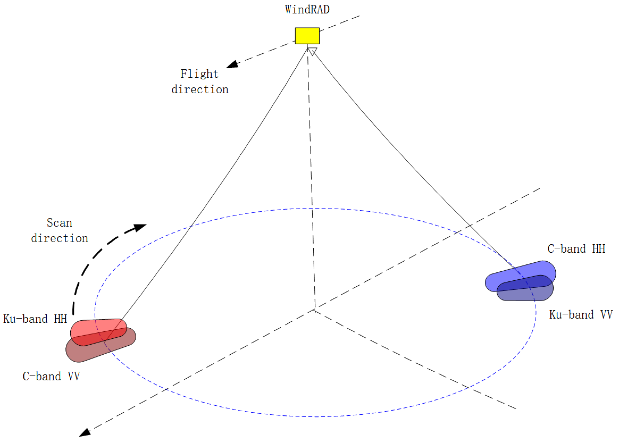
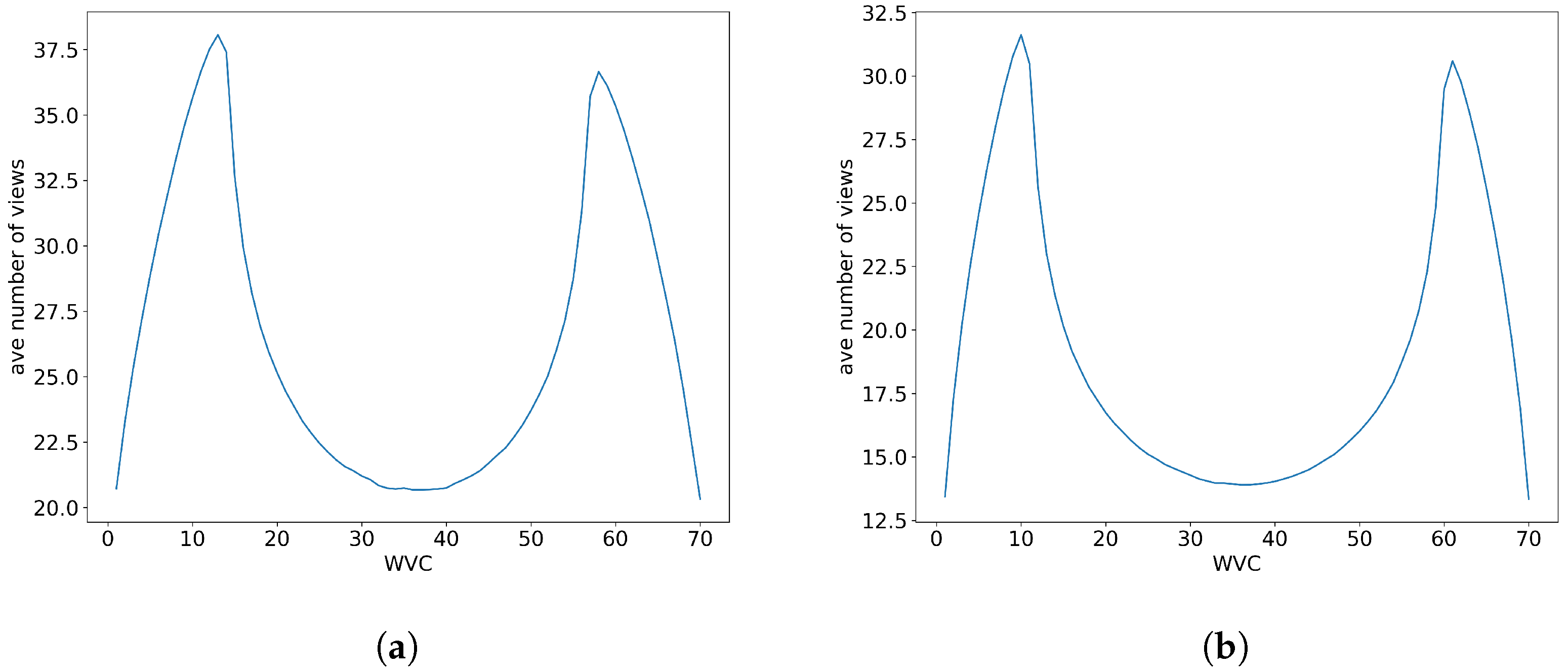
2.1.1. Geometry Distribution
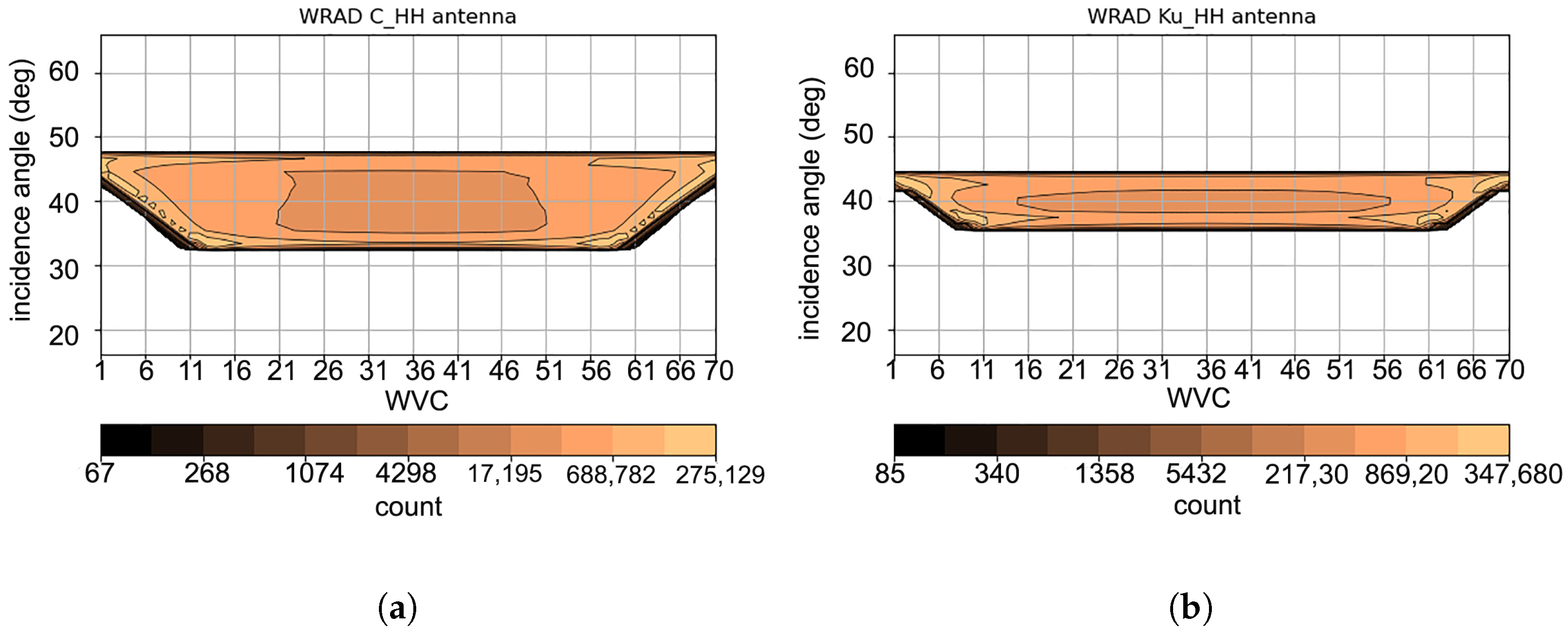
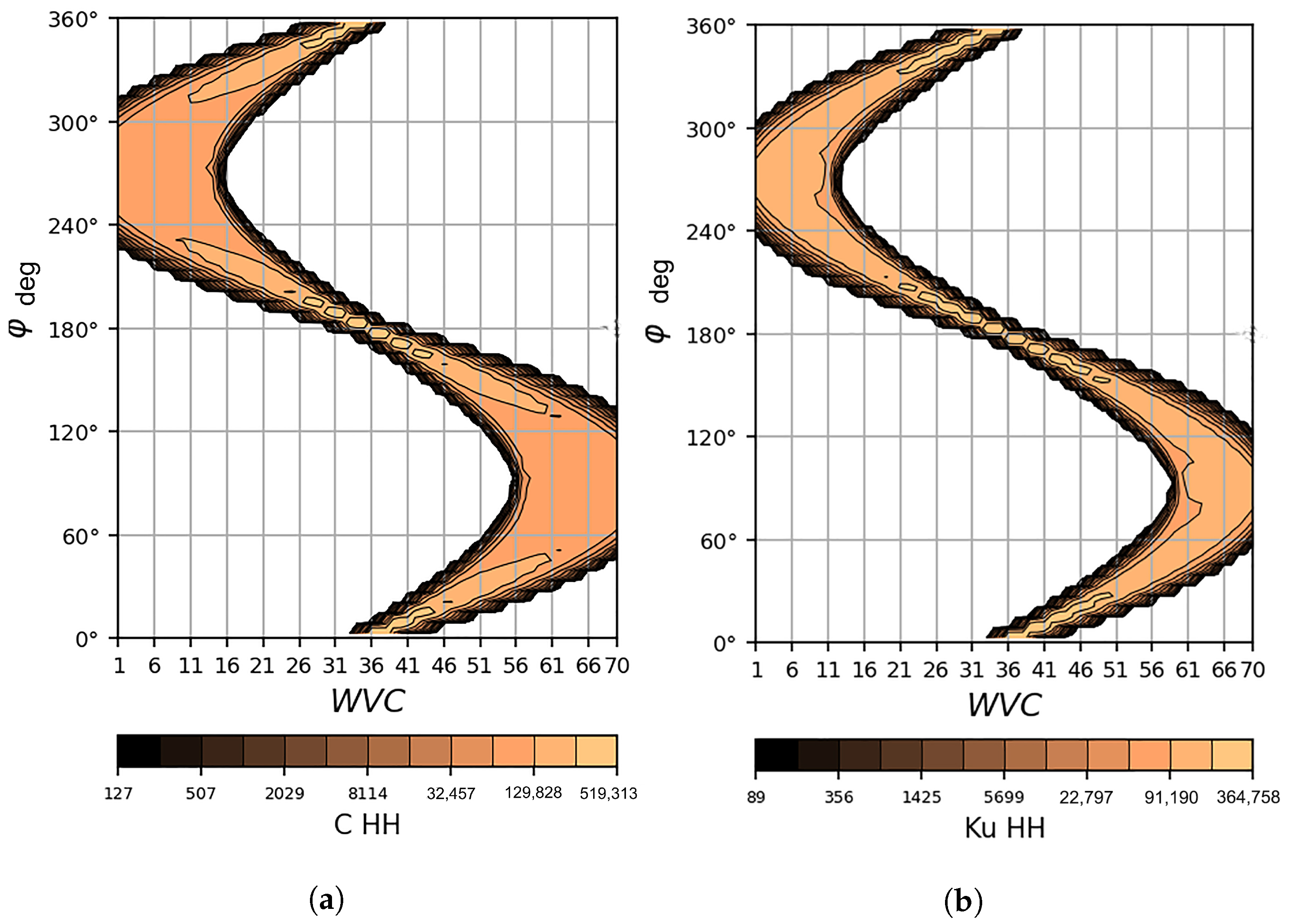
The WindRAD Level-1 data are organized in WVCs, i.e., a sub-track coordinate system is set up with axes oriented along and across the swath. The data files contain WVCs in two sizes: 20 km × 20 km, with 70 WVCs across the swath (we focus on this size in this paper), and 10 km × 10 km, with 140 WVCs across the swath. As mentioned in Section 1, WindRAD has four antennas for C-band and Ku-band frequencies; both horizontal (HH) and vertical (VV) polarizations are available, see Figure 1. The antenna beams sweep over the swath in a conical pattern, and the slices of a footprint fall in the WVCs, which leads to multiple views overlapping in each WVC at a variety of incidence angles, polarizations, and frequencies. This causes geometry to vary across the swath. The WVCs are classified into three groups: outer swath (WVC numbers 1–5 and 66–70), sweet swath (numbers 6–15 and 56–65), and nadir swath (numbers 16–55). The number of views per radar beam and WVC is shown in Figure 2. Both frequencies can have more than 30 views in the sweet swath. Although there are fewer views in the outer and nadir swaths, the number of views still exceeds 20 (C-band) and 12 (Ku-band), which is much more than with fixed fan-beam (three views) [2] and rotating pencil-beam instruments (four views) [3], though WindRAD views are much noisier and with varying spatial footprints. The number of views is also higher than that of CSCAT (9 to 10 views) [7]. Figure 3 shows the incidence angle distribution as a function of WVC number for the C-band and Ku-band beams. The C-band beam is wider than the Ku-band beam, and hence its incidence angle range is larger. Figure 4 shows the antenna azimuth angle distribution (relative to the satellite propagation direction) as a function of WVC number for C-band HH and Ku-band HH. The VV polarization distributions are very similar and not shown. From Figure 3 and Figure 4, it is clear that the outer swath contains only high incidence angles with limited azimuth angle range (around 270° and 90°), and the nadir swath contains a large range of incidence angles but only forward- or backward-looking azimuth angles, while the sweet swath contains the most diverse incidence and azimuth angle combinations. This feature makes the sweet swath the geometrically best sampled region for wind retrieval, whereas the outer and nadir swaths are more challenging.

2.1.2. σ  ° Distributions

Each WVC contains a set of  σ °s with corresponding geometry information (incidence angle, azimuth angle, polarization), called views. The distribution of  σ ° values is dependent on incidence angle. The contoured histogram plots of measured  σ ° versus simulated  σ ° per individual incidence angle are shown in Figure 5 for the Ku-band and in Figure 6 for the C-band. The simulated  σ °s are calculated using collocated ECMWF NWP stress-equivalent winds [8], view geometries (incidence and azimuth angle) and VV and HH GMF (Geophysical Model Function, NSCAT4-DS for Ku-band [9], CMOD7 for C-band VV [10], CMOD_HH for C-band HH (newly developed by Wang, private communication, 2023). Note again that the Ku-band data (v2022testKu) are from a test dataset for the period of 1 to 3 November 2022, and the C-band data (v2022operC) are the operational version for the period of 1 to 9 March 2022. Descending orbits do not show different results from ascending orbits; hence, only ascending orbits are shown here. It is clear that the  σ ° distribution at medium incidence angles has the best fit for both Ku- and C-band. The distributions at low incidence angles (Figure 5 and Figure 6a,e) for high  σ ° values are broader than those for the medium incidence angles (Figure 5 and Figure 6b,c,f,g). The deviation from the diagonal at the low incidence angles is more obvious for Ku- and C-band HH polarization, whereas the largest deviation from the diagonal is at the high incidence angles for both the Ku- and C-bands. At high incidence angles the distributions show the widest contours. The reason for these large changes in the distributions is probably that the antenna gain is strongly incidence-angle-dependent, hence  σ ° values are generally noisier at low and high incidence angles. In addition, specific quality control was applied to the upstream NRCS data provided at low and high incidence angles to exclude the  σ s with low SNR (Signal to Noise Ratio), and these quality-controlled data are excluded from the figures here, truncating and hence distorting the natural ocean NRCS distribution. Differences between HH and VV data appear to originate mainly from the different dynamic range of the  σ s. From these results, it is clear that NOC is needed to calibrate the  σ °s, and that certain restrictions should be applied on the incidence angle range to exclude undesired  σ  data in the wind inversion procedure.

2.2. Wind Inversion Algorithm

The most widely used wind inversion algorithm is based on a Bayesian approach, which is reduced to the so-called MLE (Maxima Likelihood Estimation) method [11,12,13,14,15]. We applied this approach to WindRAD, where the MLE function is defined for each WVC as:
M L E = 1 N i = 1 N ( σ m i σ s i K p ( σ x i ) ) 2 ,
Equation (1) is applied to either the C-band or Ku-band for wind retrieval; thus, the following explanation of each item in the equation represents the C-band and Ku-band, respectively. N is the number of views in the WVC,  σ m i  is the measured  σ σ s i  is the simulated  σ K p ( σ x i )  is the expected Gaussian observation noise with the form of  K p × σ x i , and  σ x i  is usually taken to be either  σ m i  or  σ s i K p  is the measurement error variance determined by instrument noise. It is included in the L1 data provided by CMA. With known incidence and azimuth angle,  σ s i  is related to wind speed and wind direction and derived through a GMF. The goal is to minimize the cost function from Equation (1) using different wind speed and direction trial values. The trial value that yields the lowest MLE is the retrieved wind vector. The details of the inversion method and wind retrieval can be found in [16,17].

3. Adapted NWP Ocean Calibration

For all scatterometers, there are general differences between the measured  σ s and simulated  σ s. These discrepancies come from instrument calibration and low-level processing, systematic, and random errors in NWP winds, as well as GMF errors. To minimize these differences, the measured  σ s need to be calibrated. A well-elaborated calibration method is NWP Ocean Calibration (NOC); it is a technique to assess the difference between the measured  σ s on one hand and simulated  σ s from collocated NWP winds with the corresponding GMF on the other hand [16,18]. NOC aligns the measurement data with the GMF by adopting a corrected instrument gain value for each incidence angle (beam pattern) and yields accurate wind retrievals, even if the original scatterometer gain value calibration is inaccurate [19]. The NOC method has been implemented successfully, not only in fixed fan-beam instruments such as ASCAT [20], but also in other types of scatterometers such as rotating pencil-beam [21] and rotating fan-beam [7] instruments. For rotating fan-beam scatterometers, NOC has been investigated with CSCAT [7]. WindRAD is also a rotating fan-beam instrument, but it has dual frequency antennas and different data characteristics compared with CSCAT. Thus, NOC needs to be thoroughly analyzed for this new configuration. In this section, both NOC as a function of incidence angle (NOCinc) and NOC as a function of incidence angle and relative antenna azimuth angle (NOCant, the relative antenna azimuth angle being the angle between the satellite direction of motion and the antenna azimuth angle) are described, assessed, and compared.
The simulated backscatter  σ  can be modelled as [22]:
σ ( θ , v , φ ) = A 0 ( v , θ ) [ 1 + A 1 ( v , θ ) c o s φ + A 2 ( v , θ ) c o s ( 2 φ ) ] ,
where  φ  is the angle between the wind direction and the antenna azimuth angle,  θ  is the incidence angle, and v is the wind speed. Thus, Equation (2) shows that the average  σ  can be determined by  A 0  with contributions from  A 1  and  A 2 . Integrating uniformly over the azimuth angle, this yields:
1 2 π 0 2 π σ ( θ , v , φ ) d φ = A 0 ( v , θ ) ,
As shown in Equation (3), when the azimuth distribution is sampled uniformly for all wind speeds and incidence angles, the mean of  A 0  is identical to the mean of  σ , which also indicates that the uncertainties  A 1  and  A 2  have no contribution to the  σ  (mean  σ ). However, in reality, the azimuth angle distribution is not uniform; in order to derive a uniform azimuth angle distribution for each speed, the collocated NWP data are split into wind speed bins (size 1 m/s) and azimuth bins (size 12 ). The  σ  is first averaged over all azimuth bins, implying a uniform azimuth distribution, and then it is weighted over all wind speed bins according to the wind speed distribution. The difference between measured  σ  and simulated  σ  is the NOC correction [7,20]. Section 3.1 and Section 3.2 describe NOCinc and NOCant respectively.
The natural variability of  σ  distributions is very large and depends on climate zone, weather variability, etc. These aspects are well predicted by NWP and, hence, can be removed by subtracting the simulated from the measured  σ . In addition, the  σ  used in NOC calculation is averaged over the corresponding bins, which further reduces the possibility of NOC corrections biased towards a specific azimuth. In order to confirm the validity of NOC calculated from only 3 days of data, tests using 3 days, 10 days, and 30 days of data were performed using an older data version. The NOC calibration coefficients differ by less than 0.03 dB between those different time periods, which indicates that 3 days of data are sufficient, and increasing the amount of data does not substantially change the NOC outcome. As mentioned in Section 2.1.2, the Ku-band data (v2022testKu) used here are available from 1–3 November 2022, and the amount of data is enough for both NOCinc and NOCant calculations. For the C-band (v2022operC), data from 1–10 March 2022 are applied for NOC calculation.

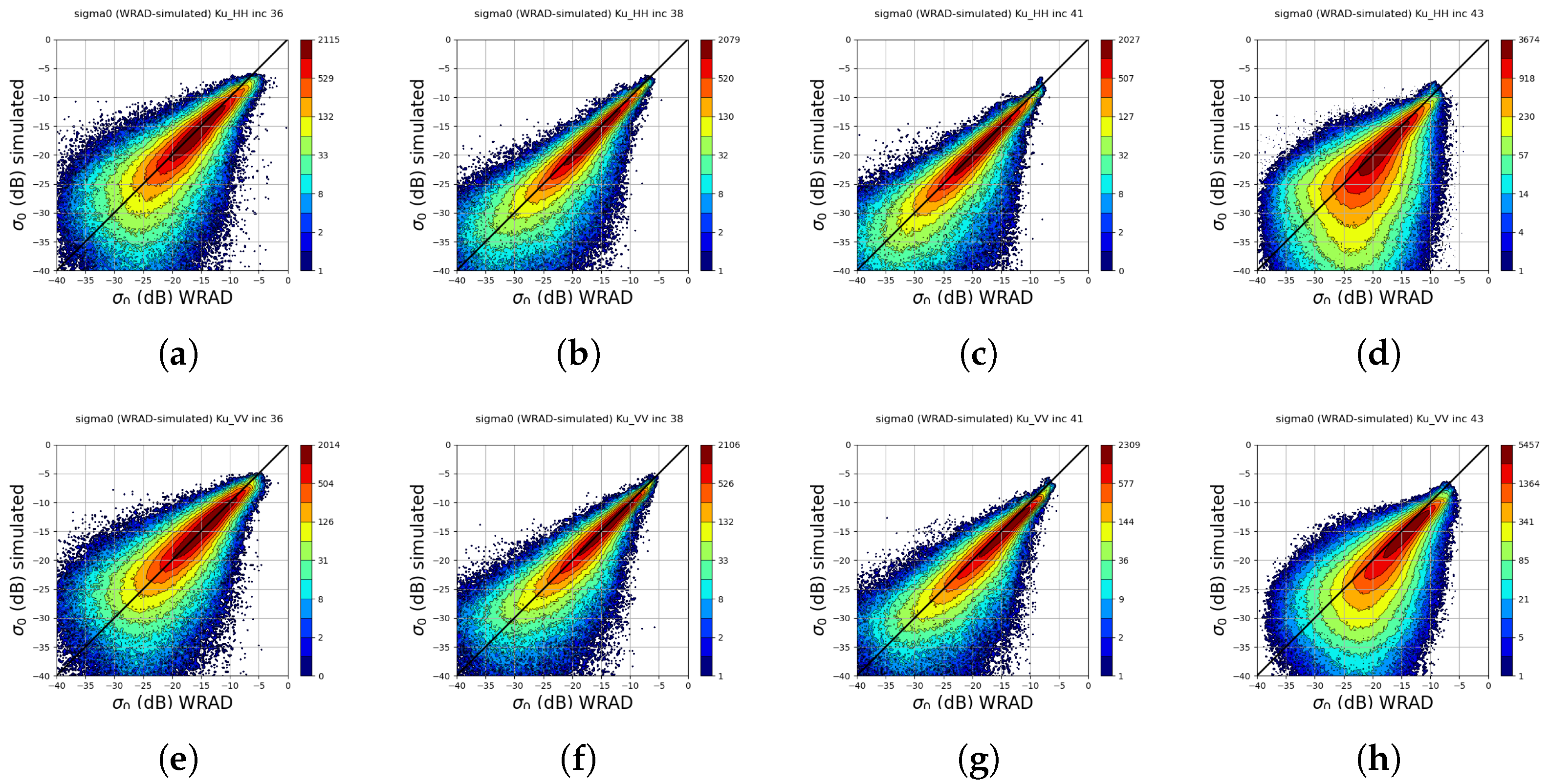
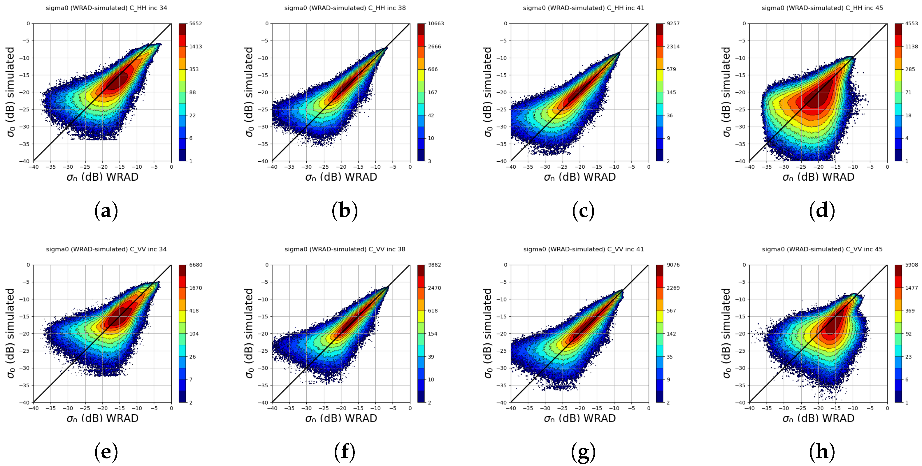
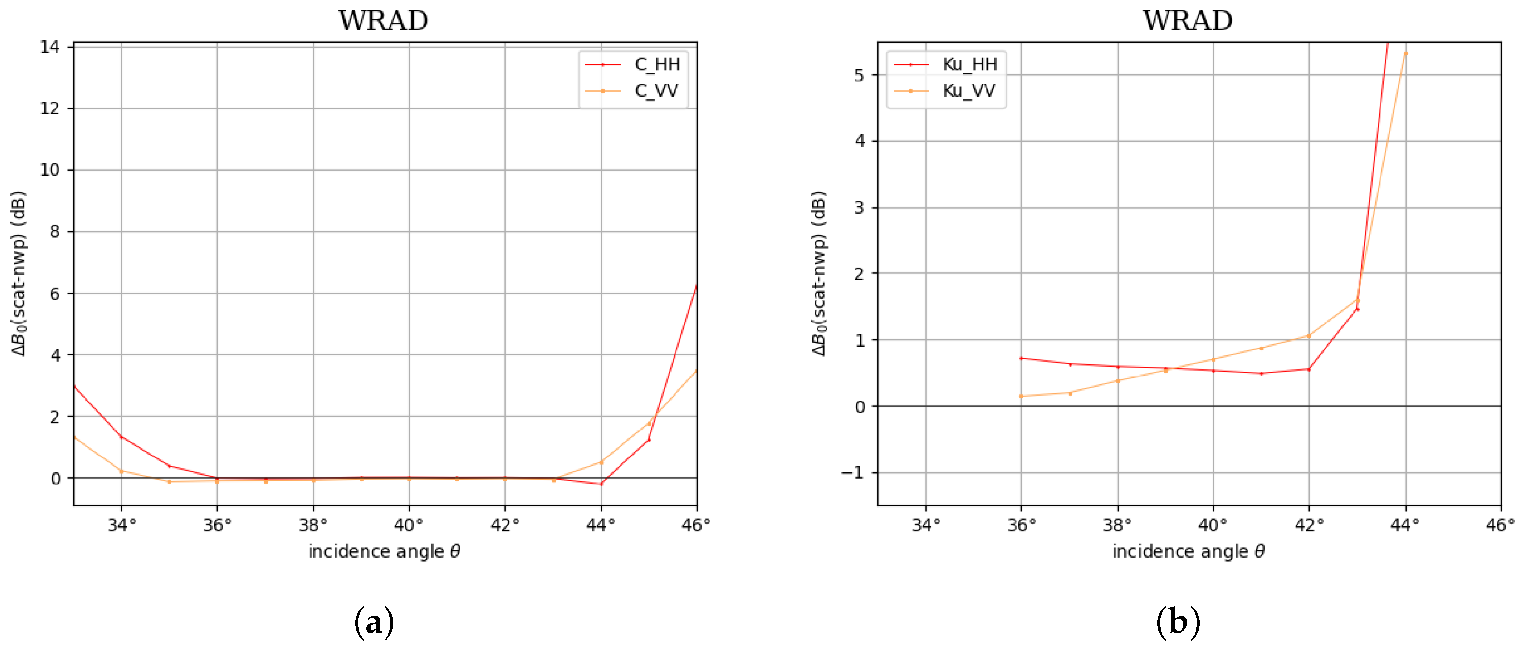
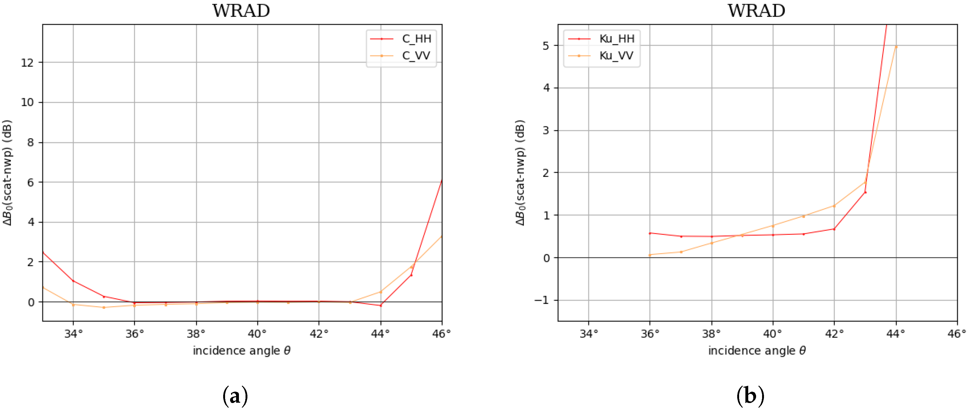
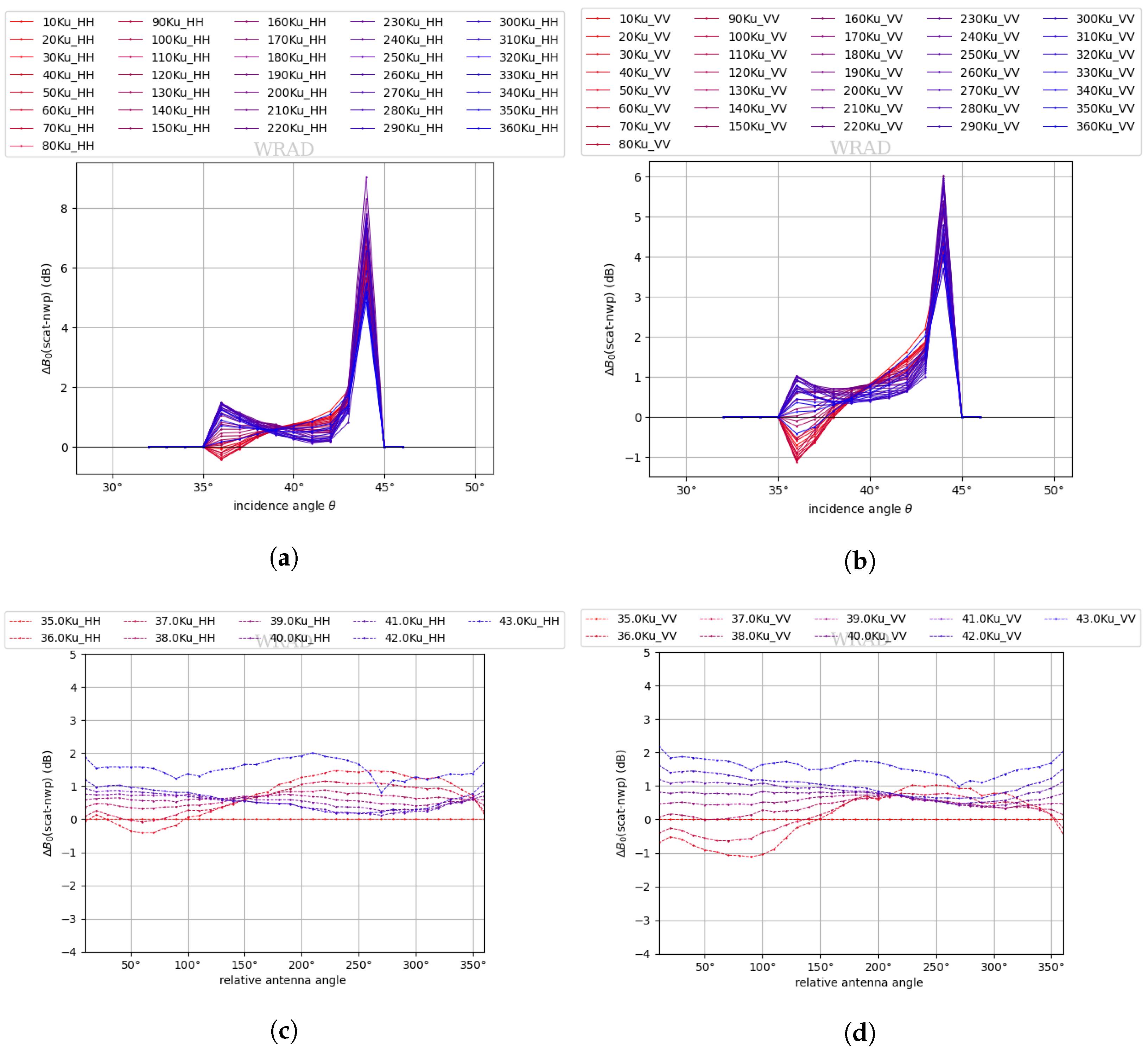
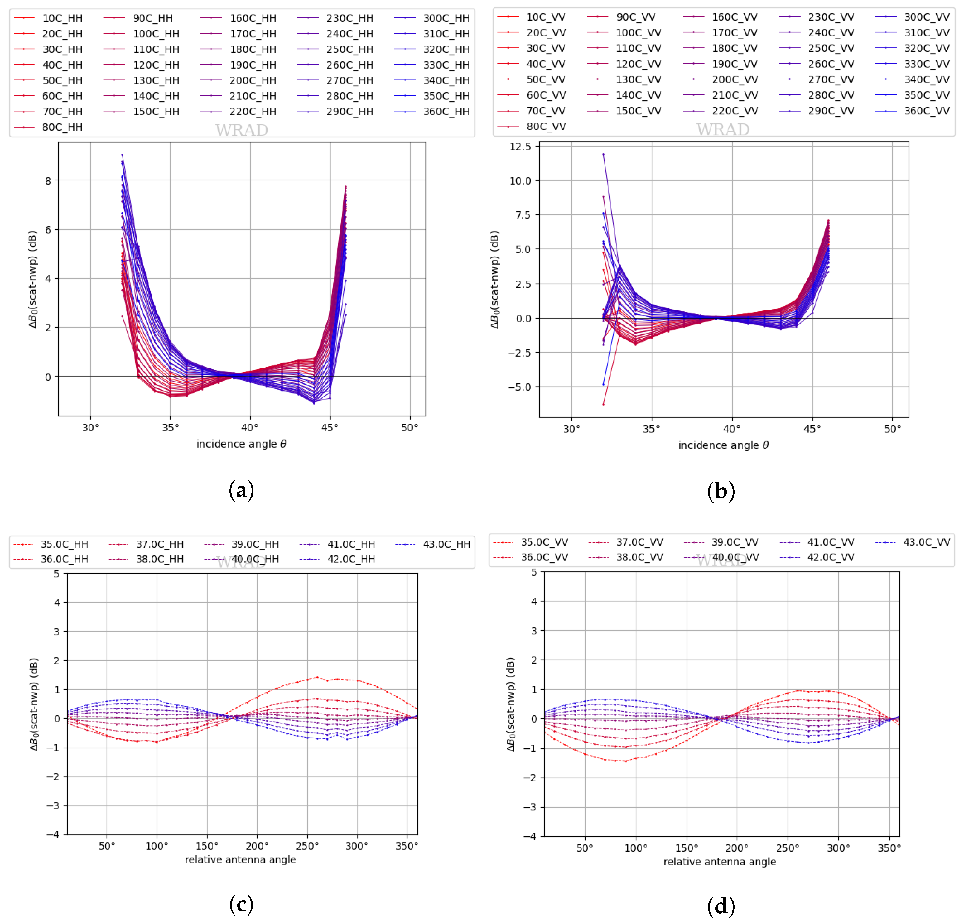
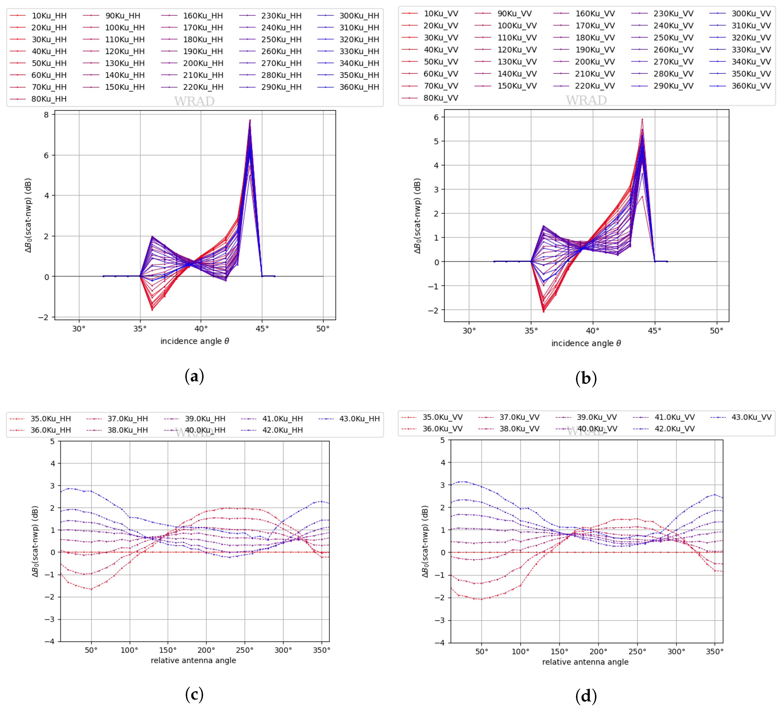
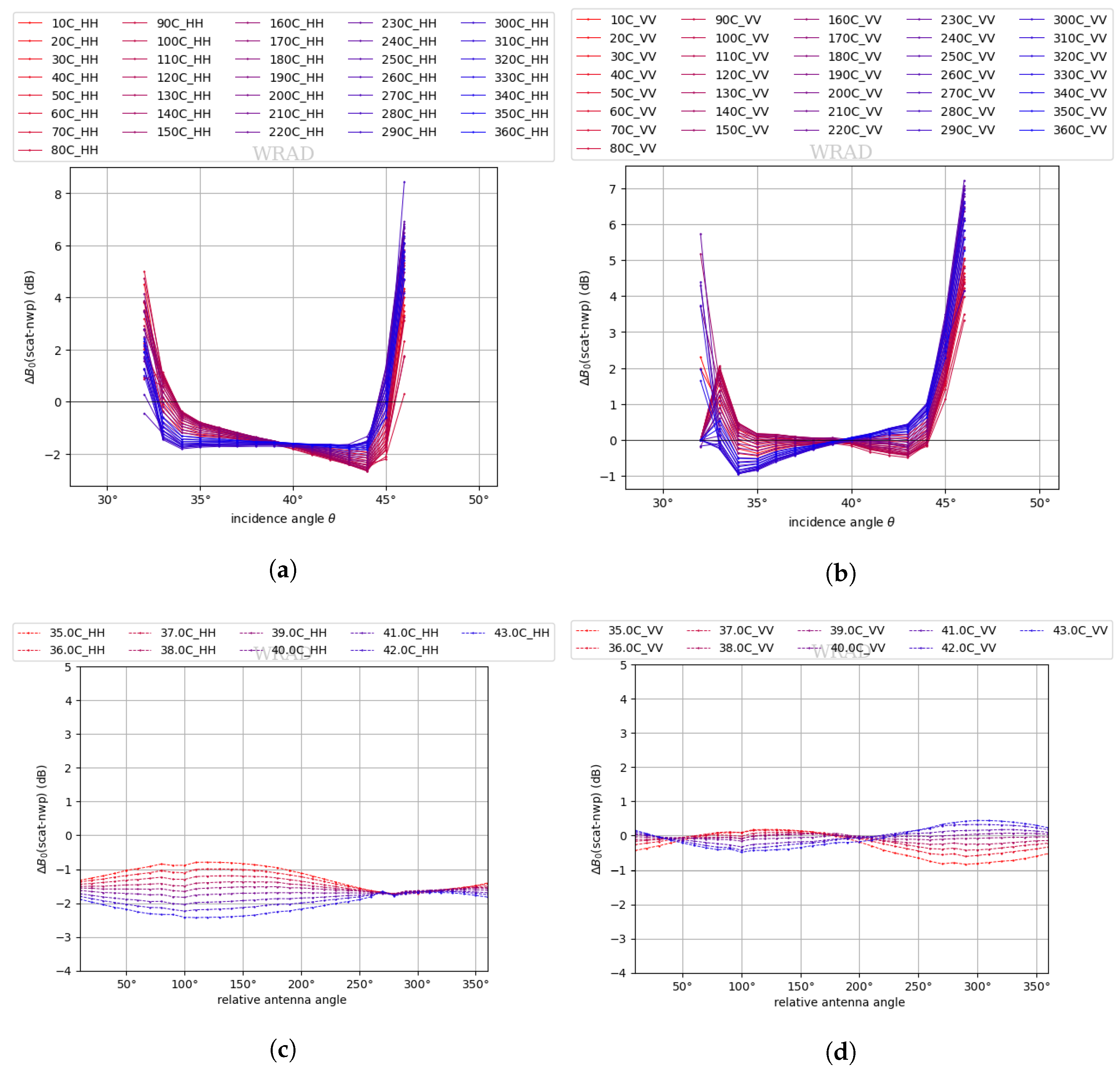
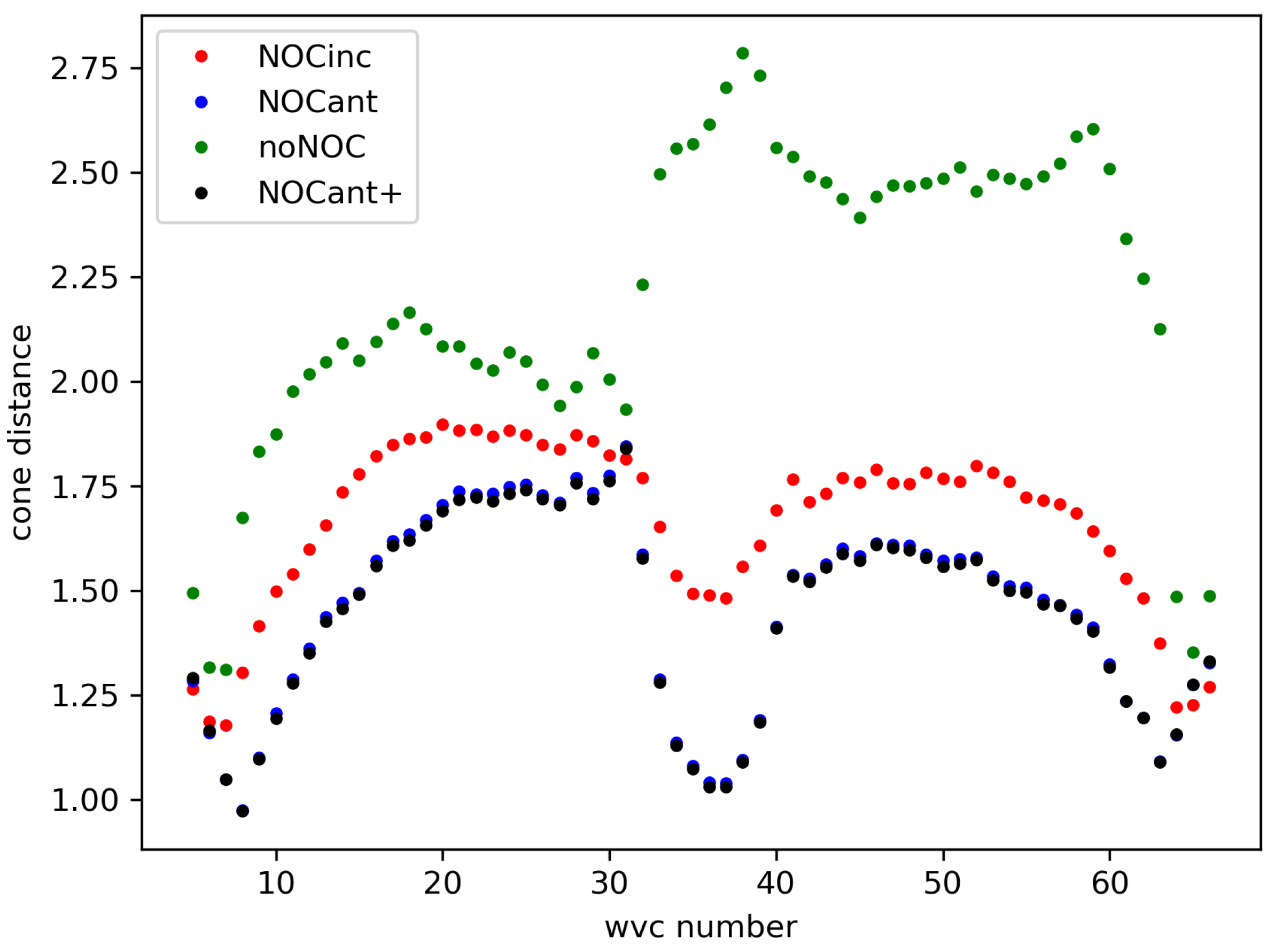
3.1. Noc as a Function of Incidence Angle: Nocinc

The NOCinc correction is the difference between measured and simulated  σ  as a function of the incidence angle for each antenna. Data are binned by incidence angle (bin size 1 ) and used as input to derive measured and simulated  σ . Figure 7 shows the NOCinc per antenna for ascending orbits: the NOCinc for the C-band is quite flat and nearly zero at the intermediate incidence angles between 36  and 43 , and it increases substantially at low and, particularly, at high incidence angles. For the Ku-band, the NOCinc varies by about 0.2 dB for the HH polarization for incidence angles below 42 , whereas it varies within a range of 1 dB for VV polarization for incidence angles below 42 . At incidence angles larger than 43 , the NOCinc increases drastically. Note that biases of 0.1 dB typically correspond to wind speed biases of about 0.1 m/s, which are typically targeted as the upper bound in global wind retrieval. As shown in Figure 5 and Figure 6, the higher the incidence angle, the more distorted the  σ  distribution is, which implies that the larger the amplitude, the higher-order corrections needed. The noise at high incidence angles is also much higher, and the amount of data at high incidence angles is much smaller, due to the quality control and hence distribution distortion; this implies that the much larger correction will not be effective in correcting the backscatter distribution at these incidence angles. The NOCinc for descending orbits shows almost the same features (Figure 8).

3.2. NOCant

NOCant is the difference between measured and simulated  σ  as a function of incidence angle and relative antenna azimuth angle (the angle between the antenna azimuth and satellite motion direction) for each antenna. The same dataset that was used for NOCinc is used again here. The data were binned by incidence angle (bin size 1 ) and relative antenna azimuth angle (bin size 10 ) to derive corresponding measured and simulated  σ .
Figure 9 and Figure 10 illustrate NOCant for the Ku- and C-band for ascending orbits. Figure 11 and Figure 12 illustrate the same for descending orbits. These figures show two perspectives: 1. NOCant as a function of incidence angle (x-axis) per relative antenna azimuth angle (upper panel); 2. NOCant as a function of relative antenna azimuth angle (x-axis) per incidence angle (lower panel).
The Ku-band in perspective 1 (Figure 9a,b) shows that the NOCant at high incidence angles (larger than 43 ) increases drastically for all relative antenna angles due to the higher noise and the smaller amount of data, whereas at incidence angles smaller than 43 , the NOCant either increases or decreases with decreasing incidence angle, depending on the relative antenna azimuth angle. By summing up the NOCant of all the relative antenna azimuth angles for a specific incidence angle (not shown), which can be roughly considered as NOCinc at that incidence angle, the values cancel out, and this leads to a rather small slope as described in Section 3.1. This suggests that the NOCinc correction is probably insufficient to correct the NRCS distributions. As shown in the Ku-band perspective 2 (Figure 9c,d), the NOCant as a function of relative antenna azimuth angle has an oscillating pattern, where ideally it should be flat to within a few tenths of a dB [7]. Wind retrieval artifacts may be anticipated if NOCinc is applied, but not NOCant. NOCant for descending orbits (Figure 11) is similar in shape to NOCant for ascending orbits (Figure 9) but with a slightly larger oscillation amplitude; this difference is canceled out in NOCinc.
The C-band NOCant (Figure 10 and Figure 12) also has an oscillating pattern similar to that of the Ku-band, but NOCant as a function of incidence angle shows opposite trends for descending orbits (Figure 12) compared with ascending orbits (Figure 10). This can be seen more clearly from the red and blue lines in the upper panels of Figure 10 and Figure 12. This feature is probably related to data reprocessing at upstream, and testing is being carried out, with the target of rectifying this in the next data version. Due to the significant NRCS differences, it is necessary to apply NOCant separately for ascending and descending orbits.
NOCant is more suitable than NOCinc for WindRAD, because NOCant unveils hidden features compared with NOCinc, and it shows that NOC for ascending and descending orbits is different, which is also not clear from NOCinc. The NOC method helps to identify and visualize basic processing problems and to correct them; this will lead to upstream data updates. The methods developed in this work will still be valid for future updated data. Section 4.1 quantifies the suitability of NOCant and NOCinc through GMF fitting.

4. Wind Retrieval Performance Evaluation and Discussion

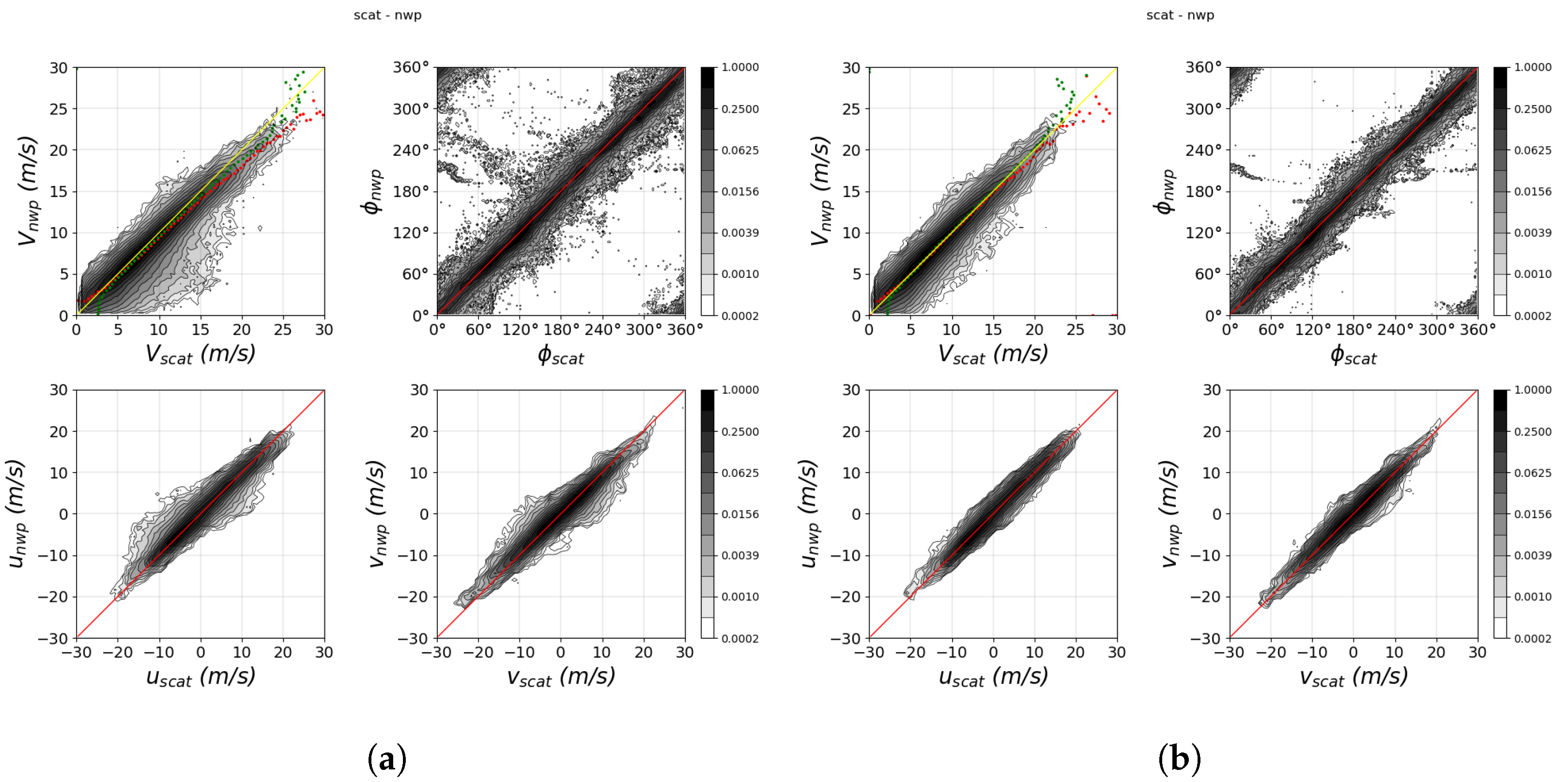
4.1. Ku-Band and C-Band GMF Fit in Measurement Space

As described in Section 3.1 and Section 3.2, NOCant is computed as a function of relative antenna azimuth angle; hence, it provides a more detailed view of the calibration corrections. NOCinc ignores the substantial effect of azimuth variation. In order to quantify the difference in wind retrieval quality between NOCinc and NOCant, the MLE (also called cone distance) from Equation (1) is used here. Equation (1) reveals how well the measurements fit the GMF. Hence, the smaller the MLE, the better the measurements fit the GMF, and better wind retrieval can be expected. The MLE is normalized by a WVC-dependent factor to obtain an expectation value of 1. This makes monitoring and quality control easier; a WVC will be flagged for quality control when its MLE is larger than a specific threshold value [13]. Different MLE normalizations and threshold values lead to different outcomes; therefore, the same normalization and threshold are applied for both NOCinc and NOCant.
The Ku-band MLE as a function of WVC is shown in Figure 13 for different cases: no NOC, NOCinc, NOCant, and NOCant+ (NOCant+ is NOCant plus a small correction value; it is discussed in Section 4.2.1). Incidence angles are limited between 36  and 42 ; backscatter data outside this range were not used in the wind retrieval. The lowest MLEs are obtained with NOCant/NOCant+; the highest MLEs are obtained when no NOC is applied. The NOCant/NOCant+ MLEs are lower than the NOCinc MLEs for almost all WVCs, except for one or two WVCs in the outer swath. This might be due to the very limited geometry diversity in the outer swath, which makes it difficult to retrieve good winds for both NOC methods. The average MLE value across the swath is 1.45 for NOCant and NOCant+, 1.67 for NOCinc, and 2.2 for no NOC. This confirms that NOCant generally results in a better fit of the measurements to the GMF than NOCinc.
The C-band MLE as a function of WVC is shown in Figure 14; for the C-band the incidence angles are limited between 36  and 43 . Similar to the Ku-band, the lowest MLEs are obtained with NOCant+/NOCant (average value 1.32/1.34), and NOCant significantly improves all WVCs except for a few nadir WVCs. The MLEs for NOCinc (average value 1.86) are only slightly lower than those for noNOC (average value 1.88). As shown in Figure 7, the NOCinc corrections between 36  and 43  are very close to zero and quite flat. This leads to a non-effective calibration, resulting in only a very small MLE difference between NOCinc and noNOC.
In summary, NOC enhances the fit of the measurements to the GMF. Additionally, NOCant further improves the fit, both for the Ku-band and C-band.

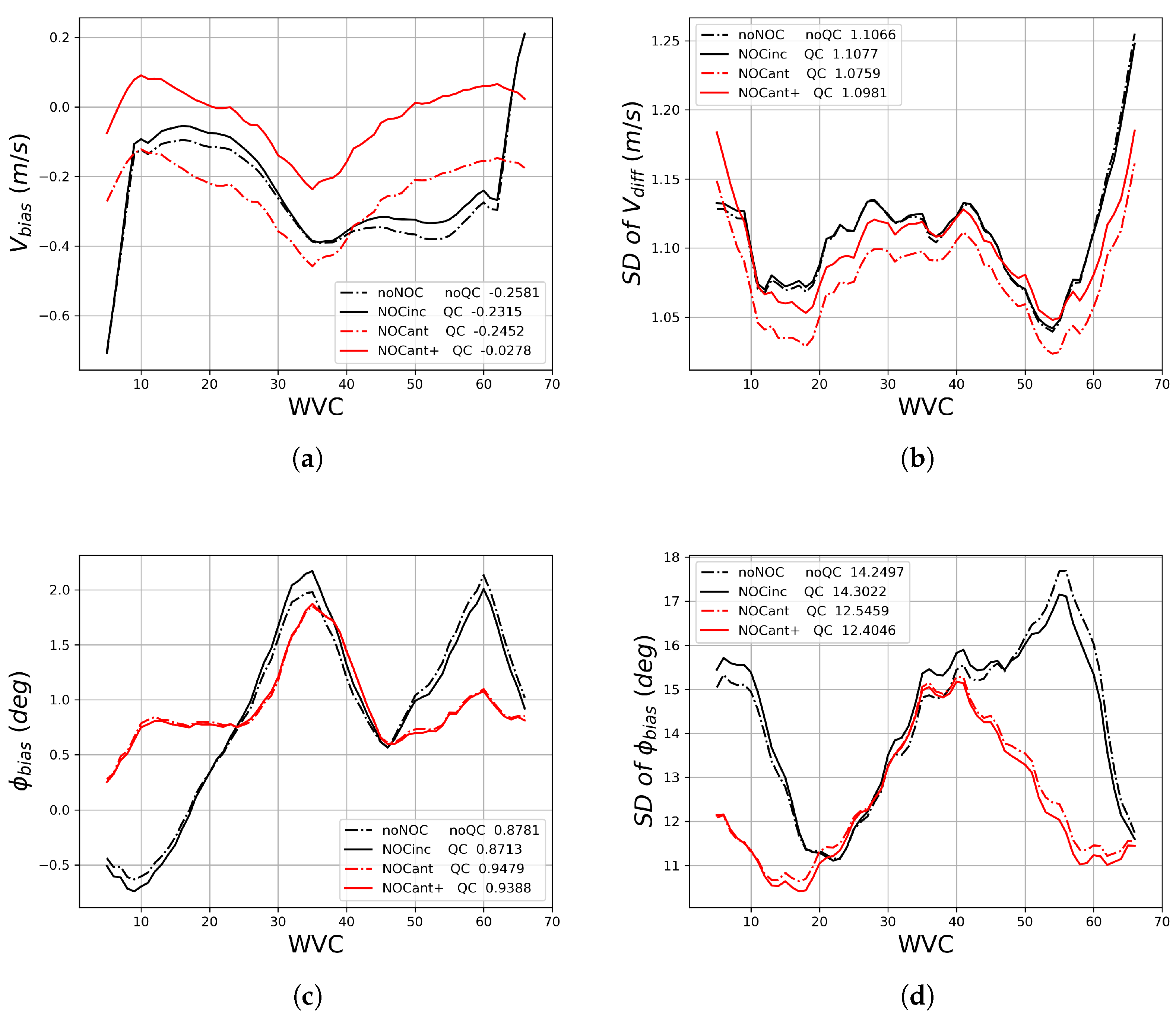
4.2. Wind Retrieval Statistics Analysis

4.2.1. Ku-Band Wind Retrieval

As described in Section 2 and Section 3 σ s at high and low incidence angles are not as accurate as those at intermediate incidence angles; hence, only incidence angles between 36  and 42  are used for Ku-band wind retrieval. MSS (Multiple Solution Scheme) [23], SST correction [9], QC (Quality Control) [24] (for removing rain contamination for the Ku-band) and 2DVAR (Two-Dimensional Variational Removal) ambiguity removal [25] have been applied in the wind inversion.
The wind retrieval result is compared against ECMWF stress-equivalent forecast winds from the operational model. Model winds are appropriate due to their spatial representativeness and high quality, which was investigated in detail in [26] for a rigorous error assessment of in-situ winds, scatterometer winds, and ECMWF model winds. Figure 15 shows the wind retrieval statistics for the Ku-band only. With NOC correction, either NOCinc or NOCant, the wind retrieval quality improves significantly compared with the noNOC case. The wind speed bias (Figure 15a) for NOCinc (black solid line) is slightly smaller than for NOCant (red dashed line), but NOCant corrects the wind speed bias better at the outermost WVCs. The wind speed SDD (Standard Deviation Difference) (Figure 15b) for NOCant is smaller than for NOCinc in the sweet and outer swaths; it is larger in the nadir swath, but only by less than 0.05 m/s. The wind direction bias (Figure 15c) has been corrected from asymmetric across the swath for NOCinc, to more symmetric for NOCant. The average wind direction SDD (Figure 15d) for NOCant is slightly reduced compared with NOCinc.
There is about −0.11 m/s residual wind speed bias for NOCant, so an engineering correction of 0.15 dB is added to the NOCant backscatter corrections (called NOCant+). The results are shown as the solid red line in Figure 15a. This extra correction reduces the average wind speed bias to −0.04 m/s and also reduces the wind speed and wind direction SDD. From Figure 15, we can conclude that NOCant+ is the best option for Ku-band wind retrieval, i.e., according to the wind validation, the highest consistency is achieved with pre-launch GMFs with NOCant+.
Figure 16 shows the retrieved winds compared with collocated ECMWF stress-equivalent winds in contoured plots for NOCant+ (including QC) and no NOC (no QC applied). The use of NOCant+ shifts the off-diagonal wind speed (Figure 16a, upper left) back to the diagonal. The use of QC reduces the rain contamination, which appears mostly as a lobe in the wind speed contour around a speed of 5–15 m/s. The wind direction ambiguity which is visible in the wind direction plots is also effectively reduced by NOCant+, resulting in more symmetric wind component scatter plots.

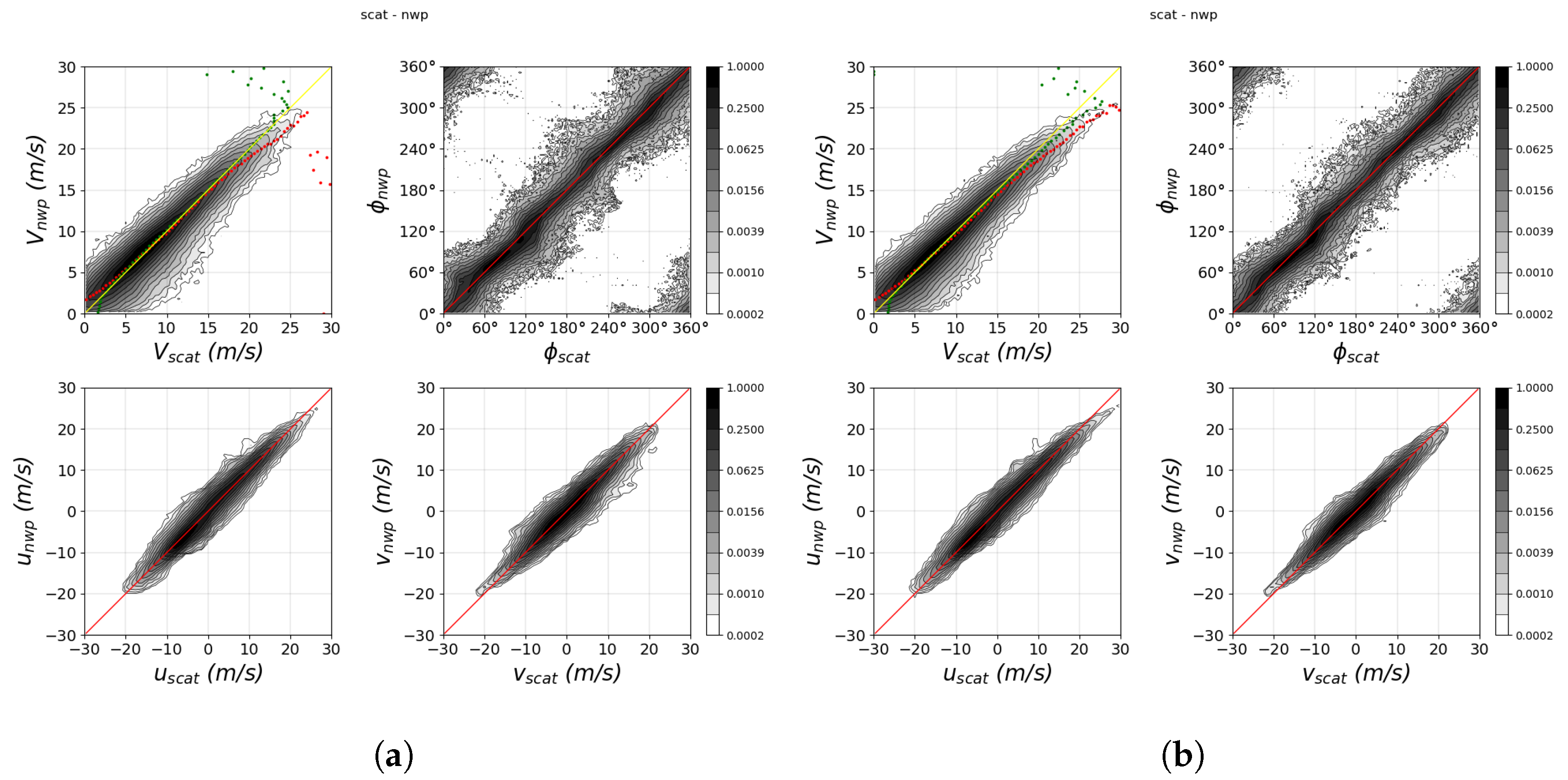
4.2.2. C-Band Wind Retrieval

Only the incidence angles between 36  and 43  are used for C-band wind retrieval. Because the C-band is not SST dependent, no SST correction is applied, while the other wind retrieval settings are the same as for the Ku-band, and wind retrieval result is also compared with ECMWF stress-equivalent winds, as described in Section 4.2.1. Figure 17 shows the wind retrieval statistics for C-band. As discussed in Section 3.1, NOCinc is probably not effective, and this is confirmed in Figure 17. The wind speed bias, wind speed SDD, wind direction bias, and the wind direction SDD of NOCinc (solid black lines) are all quite close to those of noNOC (dashed black lines); there is no significant improvement. NOCant (red dashed line) reduces the wind speed bias significantly in the outer swath, makes the wind direction bias across the swath more symmetric, and reduces the wind direction SDD by about 2 .
There is a wind speed residual of roughly −0.25 m/s for NOCant; hence, an engineering correction of 0.20 dB is added to the NOCant backscatter corrections (called NOCant+). This yields a wind speed bias of −0.03 m/s (Figure 17, red solid line). The wind speed SDD increases slightly with this extra correction, due to the implicit amplification of the retrieved speeds, but the wind direction bias and SDD do not change significantly. Hence, we choose NOCant+ as the best option for C-band wind retrieval.
Figure 18 shows the retrieved winds with collocated ECMWF model winds in contoured plots from NOCant+ and noNOC. The NOCant wind speed correlation shows narrower distributions than noNOC, and the wind direction ambiguity is reduced.

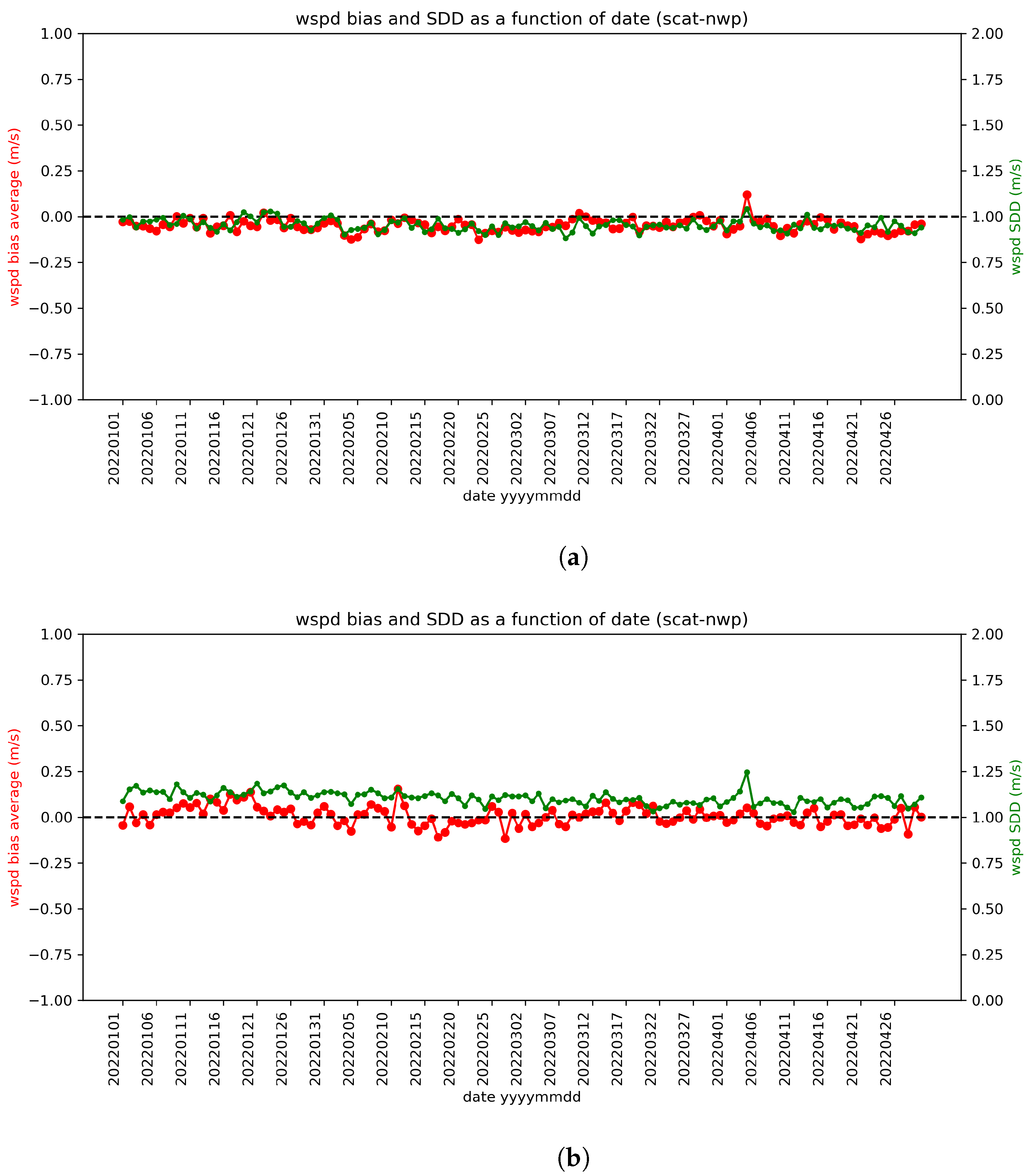
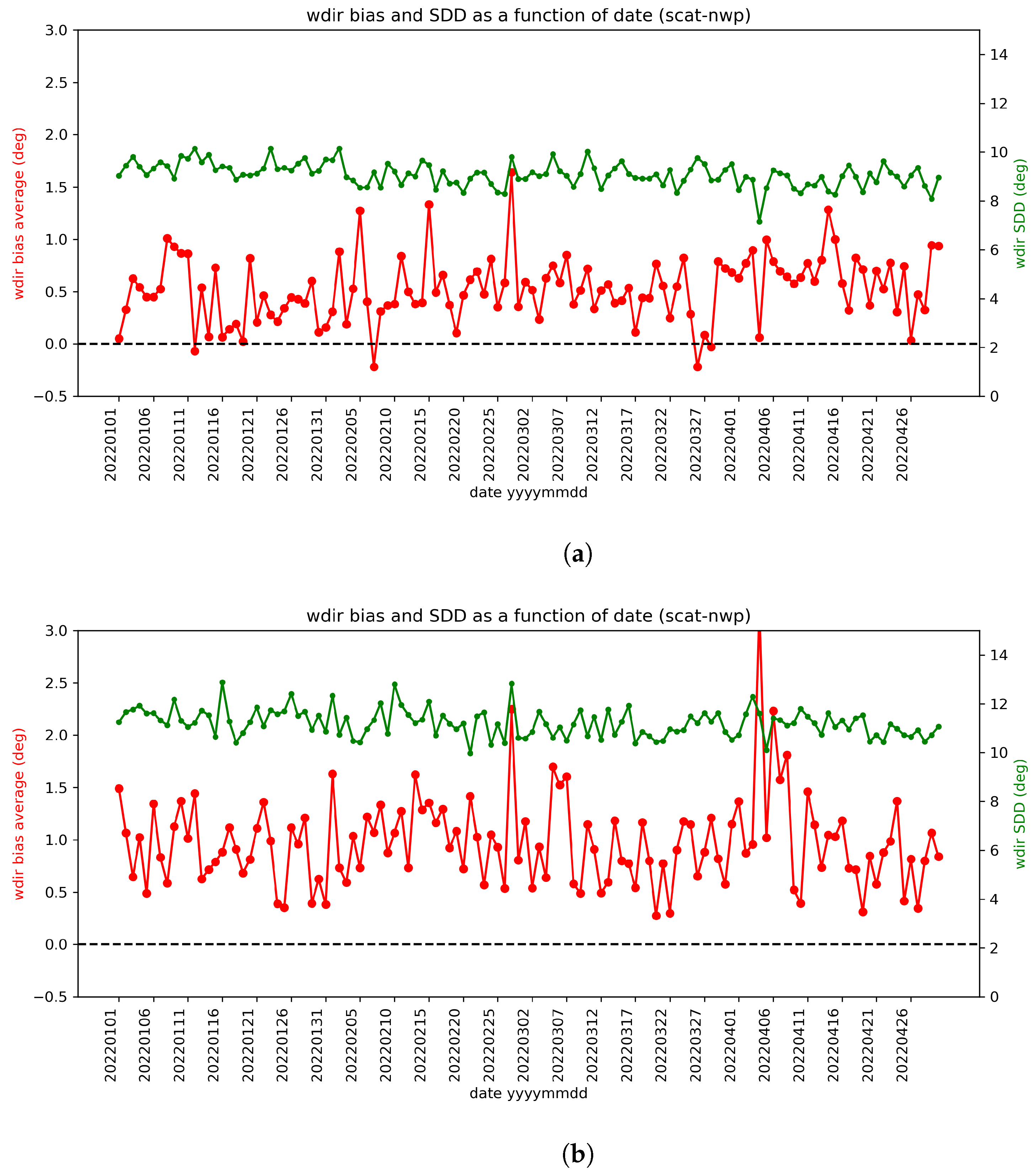
4.3. Data Stability Analysis

The backscatter data need to be stable over time in order to be useful for operational use. Figure 19 and Figure 20 show the daily average wind speed/direction biases and their SDD with respect to ECMWF stress-equivalent winds as a function of date from 1 January to 30 April 2022, for the Ku-band and C-band respectively (Note: there is no long-term data available for Ku-band version v2022testKu, thus the current operational data are applied to illustrate the instrument stability). The wind speed bias of both channels is within 0.1 m/s and the wind direction bias is in general within 1.5  over the four-month time period of the analysis, without noticeable drifts or jumps, and their corresponding SDD also indicates that the instrument is stable over time. Note that the wind speed bias and wind direction bias, as well as their corresponding SDD, are different between the Ku-band and the C-band; thus, further investigation is needed for the wind retrieval with combined channels on refined intercalibration of the  σ  and GMFs, and on noise propagation in wind retrieval.

5. Conclusions

WindRAD is the first dual-frequency rotating fan-beam scatterometer in orbit. In this paper, its data characteristics, different NOC calibration methods, and wind retrieval performance are explored. Similarly to CSCAT, the radar view geometries vary across the swaths, leading to very diverse sweet swath views and more limited view diversity in the outer and nadir swaths. The number of views for C-band is up to 37, and for Ku-band up to 31, in sweet swath WVCs. The measured  σ  distribution against simulated  σ  is distorted at high incidence angles. At low incidence angles, the  σ  distribution contour deviates from the diagonal more obviously for Ku- and C-band HH polarization. At high incidence angles, it deviates for both Ku- and C-band HH/VV polarization. The higher the incidence angle, the noisier the  σ s. Additionally, a quality control procedure was applied to the upstream data at high and low incidence angles, which distorts the  σ  distribution, preconditioned on actual noise and (low) signal characteristics. Thus, only the  σ s with incidence angles between 36  and 42  for the Ku-band, and between 36  and 43  for the C-band, are used for wind retrieval.
NOC is an essential step before wind retrieval. NOCinc corrections are rather flat and small in the selected incidence angle range, but are ineffective. NOCant takes the relative antenna azimuth angle into account. It shows that, for a specific incidence angle, the correction oscillates substantially as a function of the relative antenna azimuth angle. The sum of the NOCant corrections for all relative antenna azimuth angles (which can be roughly considered as NOCinc) is close to zero, and this explains why NOCinc values are rather small. NOCant corrections are different for ascending and descending orbits, whereas NOCinc corrections are very similar. Thus, NOCant unveils some hidden features compared with NOCinc, depending on the instrument rotation angle. The MLE furthermore shows that NOCant fits the GMF better than NOCinc does. C-band NOCant corrections show mirrored trends when comparing ascending and descending orbits, which is not the case for the Ku-band. This is because the Ku-band data used here is version v2022testKu, where the issue has been fixed in the upstream data processing. For the C-band, the version v2022operC is used, and a fix is expected in the next upstream processor update.
NOCant gives the best results for both the Ku-band and the C-band. In order to further reduce the wind speed biases, an extra engineering correction of 0.15 dB and 0.20 dB is added to Ku-band and C-band backscatter values, respectively. These calibrations are called NOCant+. NOCant+ reduces the absolute wind speed bias to less than 0.05 m/s for both individual channels, without increasing the wind speed SDD and wind direction SDD. Further investigation on combining the C-band and Ku-band data becomes relevant after the next upstream data update. Data stability over time is important for the operational use of the wind data and is confirmed using four months of the operational Ku-band and C-band data. The average daily wind speed bias of both channels is within 0.1 m/s over this period, with no data drifting or unexpected behavior.
WindRAD was launched more than a year ago, and processing improvements are in development. Further investigation is needed with the upcoming data versions; this paper gives an analysis of today’s promising status and can be considered as a reference for further research. Research topics for the future are: 1. combined C- and Ku-band retrieval; 2. the Ku-band backscatter is influenced by rain, but C-band is not, so the study of rain contamination with combined Ku-band and C-band is of interest; 3. combining the differing spatial footprints in a WVC for the nadir and outer swaths, including differing noise properties, cf. [27], to investigate resolution enhancement; 4. the optimization of the MLE cost function to take account of the local wind vector sensitivity in a WVC view geometry, cf. [15]; 5. the development of sea ice screening and a sea ice product; and 6. extension of retrieved wind fields closer to the coast, cf. [28].

Author Contributions

Conceptualization, Z.L., A.V. and A.S.; methodology, Z.L.; software, Z.L. and A.V.; validation, Z.L.; formal analysis, Z.L.; investigation, Z.L.; resources, Z.L., A.V., J.S. and F.D.; data curation, Z.L. and A.V.; writing—original draft preparation, Z.L.; writing—review and editing, A.V., A.S., J.S. and F.D.; visualization, Z.L.; supervision, A.V. and A.S.; project administration, Z.L., A.V. and A.S.; funding acquisition, A.S., Z.L., J.S. and F.D. All authors have read and agreed to the published version of the manuscript.

Funding

This research was supported by EUMETSAT OSI SAF CDOP4 (Darmstadt, Germany) and Fengyun Satellite Application Pilot Plan (FY-APP-2021.0510 China).

Data Availability Statement

Data can be acquired through the data distribution center of CMA: http://data.cma.cn/en, accessed on 12 April 2023.

Acknowledgments

We acknowledge the support of CMA in providing the data, status, and mission information. The support from the EUMETSAT Ocean and Sea Ice Satellite Application Facility is also much appreciated. We also thank Zhixiong Wang from Nanjing University of Information Science & Technology for his contribution to C-HH GMF.

Conflicts of Interest

The authors declare no conflict of interest. The funders had no role in the design of the study; in the collection, analyses, or interpretation of data; in the writing of the manuscript; or in the decision to publish the results.

Abbreviations

The following abbreviations are used in this manuscript:
ASCATAdvanced Scatterometer
CSCATCFOSAT (Chinese-French Oceanography Satellite) Scatterometer
FYFeng Yun
GMFGeophysical Model Function
HYHai Yang
MSSMultiple Solution Scheme
NOCNWP Ocean Calibration
NWPNumerical Weather Prediction
QCQuality Control
SDStandard Deviation
SDDStandard Deviation Difference
SNRSignal and Noise Ratio
SSTSea Surface Temperature
WindRADWind Radar
WVCWind Vector Cell
2DVAR2-Dimensional Variational Removal

References

  1. Zhang, P.; Hu, X.; Lu, Q.; Zhu, A.; Lin, M.; Sun, L.; Chen, L.; Xu, N. FY-3E: The First Operational Meteorological Satellite Mission in an Early Morning Orbit. Adv. Atmos. Sci. 2022, 39, 1–8. [Google Scholar] [CrossRef]
  2. Gelsthorpe, R.V.; Schied, E.; Wilson, J.J.W. ASCAT - Metop’s advanced scatterometer. Esa-Bull.-Eur. Space Agency 2000, 102, 19–27. [Google Scholar]
  3. Jiang, X.; Lin, M.; Liu, J.; Zhang, Y.; Xie, X.; Peng, H.; Zhou, W. The HY-2 satellite and its preliminary assessment. Int. J. Digit. Earth 2012, 5, 266–281. [Google Scholar] [CrossRef]
  4. Chakraborty, P.; Jyoti, R.; Gupta, P. An Advanced Ku-band Fine-Resolution and High-Sensitivity Wind Scatterometer. IEEE Trans. Geosci. Remote. Sens. 2023, 1. [Google Scholar] [CrossRef]
  5. Li, Z.; Stoffelen, A.; Verhoef, A. A Generalized Simulation Capability for Rotating Beam Scatterometers. Atmos. Meas. Tech. 2019, 12, 3573–3594. [Google Scholar] [CrossRef] [Green Version]
  6. Liu, J.; Lin, W.; Dong, X.; Lang, S.; Yun, R.; Zhu, D.; Zhang, K.; Sun, C.; Mu, B.; Ma, J.; et al. First Results from the Rotating Fan Beam Scatterometer Onboard CFOSAT. IEEE Trans. Geosci. Remote Sens. 2020, 58, 8793–8806. [Google Scholar] [CrossRef]
  7. Li, Z.; Stoffelen, A.; Verhoef, A.; Verspeek, J. Numerical Weather Prediction Ocean Calibration for the Chinese-French Oceanography Satellite Wind Scatterometer and Wind Retrieval Evaluation. Earth Space Sci. 2021, 8, e2020EA001606. [Google Scholar] [CrossRef]
  8. De Kloe, J.; Stoffelen, A.; Verhoef, A. Improved Use of Scatterometer Measurements by Using Stress-Equivalent Reference Winds. IEEE J. Sel. Top. Appl. Earth Obs. Remote Sens. 2017, 10, 2340–2347. [Google Scholar] [CrossRef]
  9. Wang, Z.; Stoffelen, A.; Zhao, C.; Vogelzang, J.; Verhoef, A.; Verspeek, J.; Lin, M.; Chen, G. An SST-dependent Ku-band geophysical model function for RapidScat. J. Geophys. Res. Ocean. 2017, 122, 3461–3480. [Google Scholar] [CrossRef]
  10. Stoffelen, A.; Verspeek, J.A.; Vogelzang, J.; Verhoef, A. The CMOD7 Geophysical Model Function for ASCAT and ERS Wind Retrievals. IEEE J. Sel. Top. Appl. Earth Obs. Remote Sens. 2017, 10, 2123–2134. [Google Scholar] [CrossRef]
  11. Chi, C.Y.; Li, F.K. A comparative study of several wind estimation algorithms for spaceborne scatterometers. IEEE Trans. Geosci. Remote Sens. 1988, 26, 115–121. [Google Scholar] [CrossRef]
  12. Pierson, W.J. Probabilities and statistics for backscatter estimates obtained by a scatterometer. J. Geophys. Res. 1989, 94, 9743–9759. [Google Scholar] [CrossRef]
  13. Portabella, M.; Stoffelen, A. Characterization of Residual Information for SeaWinds Quality Control. IEEE Trans. Geosci. Rem. Sens. 2002, 40, 2747–2759. [Google Scholar] [CrossRef]
  14. Cornford, D.; Csató, L.; Evans, D.J.; Opper, M. Bayesian Analysis of the Scatterometer Wind Retrieval Inverse Problem: Some New Approaches. J. R. Stat. Soc. Ser. B Stat. Methodol. 2004, 66, 609–652. [Google Scholar] [CrossRef]
  15. Stoffelen, A.; Portabella, M. On Bayesian Scatterometer Wind Inversion. IEEE Trans. Geosci. Remote Sens. 2006, 44, 1523–1533. [Google Scholar] [CrossRef]
  16. Stoffelen, A.; Anderson, D. Scatterometer data interpretation: Measurement space and inversion. J. Atmos. Ocean. Technol. 1997, 14, 1298–1313. [Google Scholar] [CrossRef]
  17. Vogelzang, J.; Stoffelen, A. Improvements in Ku-band scatterometer wind ambiguity removal using ASCAT-based empirical background error correlations. Q. J. R. Meteorol. Soc. 2018, 144, 2245–2259. [Google Scholar] [CrossRef]
  18. Freilich, M.H.; Qi, H.; Dunbar, R.S. Scatterometer Beam Balancing Using Open-Ocean Backscatter Measurements. J. Atmos. Ocean. Technol. 1999, 16, 283–297. [Google Scholar] [CrossRef]
  19. Stofflen, A. A Simple Method for Calibration of a Scatterometer over the Ocean. J. Atmos. Ocean. Technol. 1999, 16, 275–282. [Google Scholar] [CrossRef]
  20. Verspeek, J.; Stoffelen, A.; Verhoef, A.; Portabella, M. Improved ASCAT wind retrieval using NWP ocean calibration. IEEE Trans. Geosci. Remote Sens. 2012, 50, 2488–2494. [Google Scholar] [CrossRef] [Green Version]
  21. Yun, R.; Stofflen, A.; Verspeek, J.; Verhoef, A. NWP ocean calibration of Ku-band scatterometers. In Proceedings of the IEEE International Geoscience and Remote Sensing Symposium, Munich, Germany, 22–27 July 2012. [Google Scholar] [CrossRef]
  22. Wentz, F.J.; Smith, D.K. A model function for the ocean-nornalized radar cross section at 14 GHz derived from NSCAT observatioen. J. Geophys. Res. 1999, 104, 11499–11514. [Google Scholar] [CrossRef]
  23. Portabella, M. Wind Field Retrieval from Satellite Radar Systems. Ph.D. Thesis, University of Barcelona, Barcelona, Spain, 2002. [Google Scholar]
  24. Portabella, M.; Stoffelen, A. Rain Detection and Quality Control of SeaWinds. J. Atmos. Ocean. Technol. 2001, 18, 1171–1183. [Google Scholar] [CrossRef]
  25. Vogelzang, J.; Verhoef, A.; De Vries, J.; Bonekamp, H. Validation of Two-Dimensional Variational Ambiguity Removal on SeaWinds Scatterometer Data. J. Atmos. Ocean. Technol. 2009, 26, 1229–1245. [Google Scholar] [CrossRef]
  26. Vogelzang, J.; Stoffelen, A. On the Accuracy and Consistency of Quintuple Collocation Analysis of In Situ, Scatterometer, and NWP Winds. Remote Sens. 2022, 14, 4552. [Google Scholar] [CrossRef]
  27. Vogelzang, J.; Stoffelen, A. ASCAT Ultrahigh-Resolution Wind Products on Optimized Grids. IEEE J. Sel. Top. Appl. Earth Obs. Remote Sens. 2017, 10, 2332–2339. [Google Scholar] [CrossRef]
  28. Grieco, G.; Portabella, M.; Vogelzang, J.; Verhoef, A.; Stoffelen, A. Initial Development of Pencil-Beam Scatterometer Coastal Processing; Technical Report; Royal Netherlands Meteorological Institute: De Bilt, The Netherlands, 2020. [Google Scholar]
Figure 1. WindRAD rotating fan-beam illustration.
Remotesensing 15 02087 g001
Figure 2. Average number of views as a function of WVC: (a) C-band HH and VV beams. (b) Ku-band HH and VV beams.
Remotesensing 15 02087 g002
Figure 3. Incidence angle distribution as a function of WVC: (a) C-band HH. (b) Ku-band HH.
Remotesensing 15 02087 g003
Figure 4. Azimuth angle distribution as a function of WVC: (a) C-band HH. (b) Ku-band HH.
Remotesensing 15 02087 g004
Figure 5. Joint distribution of Ku-band measured  σ ° and simulated  σ °, ascending orbits, date 1 November 2022–3 November 2022, HH (upper panel), VV (lower panel): (a,e) incidence angle 36°; (b,f) incidence angle 38°; (c,g) incidence angle 41°; (d,h) incidence angle 43°.
Remotesensing 15 02087 g005
Figure 6. Joint distribution of C-band measured  σ ° and simulated  σ °, ascending orbits, date 1 March 2022–9 March 2022, HH (upper panel), VV (lower panel): (a,e) incidence angle 34°; (b,f) incidence angle 38°; (c,g) incidence angle 41°; (d,h) incidence angle 45°.
Remotesensing 15 02087 g006
Figure 7. NOC as a function of incidence angle for ascending orbits: (a) C-band HH and VV polarization; (b) Ku-band HH and VV polarization.
Remotesensing 15 02087 g007
Figure 8. NOC as a function of incidence angle for descending orbits: (a) C-band HH and VV polarization; (b) Ku-band HH and VV polarization.
Remotesensing 15 02087 g008
Figure 9. Ku-band NOCant (NOC as a function of incidence angle and relative antenna angle) for ascending orbits. The upper panel is as a function of incidence angle (x-axis) per relative antenna angle (red to blue lines), the lower panel is as a function of relative antenna angle (x-axis) per incidence angle (red to blue lines): (a,c) HH polarization; (b,d) VV polarization.
Remotesensing 15 02087 g009
Figure 10. C-band NOCant (NOC as a function of incidence angle and relative antenna angle) for ascending orbits. The upper panel is as a function of incidence angle (x-axis) per relative antenna angle (red to blue lines), the lower panel is as a function of relative antenna angle (x-axis) per incidence angle (red to blue lines): (a,c) HH polarization; (b,d) VV polarization.
Remotesensing 15 02087 g010
Figure 11. Ku-band NOCant (NOC as a function of incidence angle and relative antenna angle) for descending orbits. The upper panel is as a function of incidence angle (x-axis) per relative antenna angle (red to blue lines), the lower panel is as a function of relative antenna angle (x-axis) per incidence angle (red to blue lines): (a) and (c) HH polarization; (b) and (d) VV polarization.
Remotesensing 15 02087 g011
Figure 12. C-band NOCant (NOC as a function of incidence angle and relative antenna angle) for descending orbits. The upper panel is as a function of incidence angle (x-axis) per relative antenna angle (red to blue lines), the lower panel is as a function of relative antenna angle (x-axis) per incidence angle (red to blue lines): (a,c) HH polarization; (b,d) VV polarization.
Remotesensing 15 02087 g012
Figure 13. Average MLE (cone distance) as a function of WVC for Ku-band ascending orbits with respect to NSCAT4-DS [9] (noNOC is green, NOCinc is red, NOCant is blue, NOCant+ is black).
Remotesensing 15 02087 g013
Figure 14. Average MLE (cone distance) as a function of WVC for C-band ascending orbits (noNOC is green, NOCinc is red, NOCant is blue, NOCant+ is black).
Remotesensing 15 02087 g014
Figure 15. Ku-band ascending orbits wind retrieval statistics as a function of WVC with noNOC, NOCinc, NOCant, NOCant+. SST correction and QC are applied, and the mean numbers of each condition are stated beside each legend, data from 1 November 2022–3 November 2022: (a) wind speed bias, (b) wind speed SDD, (c) wind direction bias, (d) wind direction SDD.
Remotesensing 15 02087 g015
Figure 16. Ku-band ascending orbits: contoured wind speed, wind direction (wind speed > 4 m/s), u/v components histograms of retrieved winds vs. ECMWF winds, data from 1 November 2022–3 November 2022: (a) no NOC, (b) NOCant+0.15dB with QC. In the wind speed contour, the red dotted line is the average ECMWF wind speed, the green dotted line is the average WindRAD wind, and the yellow straight line is the diagonal.
Remotesensing 15 02087 g016
Figure 17. C-band ascending orbits wind retrieval statistics as a function of WVC with noNOC, NOCinc, NOCant, NOCant+. The mean numbers of each condition are stated beside each legend, data from 1–9 March 2022: (a) wind speed bias, (b) wind speed SDD, (c) wind direction bias, (d) wind direction SDD.
Remotesensing 15 02087 g017
Figure 18. C-band ascending orbits: contoured wind speed, wind direction (wind speed > 4 m/s), u/v components histograms of retrieved winds vs. ECMWF winds, data from 1–9 March 2022: (a) noNOC, (b) NOCant+. In the wind speed contour, the red dotted line is the average ECMWF wind speed, the green dotted line is the average WindRAD wind, and the yellow straight line is the diagonal.
Remotesensing 15 02087 g018
Figure 19. Wind speed bias and its SDD as a function of date (with NOCant+), from 1 January to 30 April 2022: (a) Ku-band, (b) C-band.
Remotesensing 15 02087 g019
Figure 20. Wind direction bias and its SDD as a function of date (with NOCant+), from 1 January to 30 April 2022: (a) Ku-band, (b) C-band.
Remotesensing 15 02087 g020
Disclaimer/Publisher’s Note: The statements, opinions and data contained in all publications are solely those of the individual author(s) and contributor(s) and not of MDPI and/or the editor(s). MDPI and/or the editor(s) disclaim responsibility for any injury to people or property resulting from any ideas, methods, instructions or products referred to in the content.

