

Driving Mechanism of Differentiation in Urban Thermal Environment during Rapid Urbanization
by
 , , ,
, , ,
Yifeng Ji
1,
You Peng
2,
Zhitao Li
3,
Jiang Li
1,
Shaobo Liu
1,*,
Xiaoxi Cai
4,
Yicheng Yin
5 and
Tao Feng
6 1
Department of Environmental Design, School of Architecture and Art, Central South University, Changsha 410083, China
2
Urban Planning and Transportation Research Group, Department of the Built Environment, Eindhoven University of Technology, P.O. Box 513, 5600 MB Eindhoven, The Netherlands
3
Smart Transport Key Laboratory of Hunan Province, School of Traffic and Transportation Engineering, Central South University, Changsha 410075, China
4
Department of Environmental Design, College of Art and Design, Hunan First Normal University, Changsha 410205, China
5
Department of Urban and Rural Planning, School of Architecture and Planning, Hunan University, Changsha 410082, China
6
Urban and Data Science Lab, Graduate School of Advanced Science and Engineering, Hiroshima University, Higashi Hiroshima 739-8529, Japan
*
Author to whom correspondence should be addressed.
Remote Sens. 2023, 15(8), 2075; https://doi.org/10.3390/rs15082075
Submission received: 7 March 2023
/
Revised: 11 April 2023
/
Accepted: 12 April 2023
/
Published: 14 April 2023
(This article belongs to the Topic Climate Change and Environmental Sustainability, 2nd Volume)
Abstract
:To achieve sustainable urban development, it is essential to gain insight into the spatial and temporal differentiation characteristics and the driving mechanisms of the urban thermal environment (UTE). As urbanization continues to accelerate, human activity and landscape configuration and composition interact to complicate the UTE. However, the differences in UTE-driven mechanisms at different stages of urbanization remain unclear. In this study, the UTE of Shenyang was measured quantitatively by using the land surface temperature (LST). The spatial and temporal differentiation characteristics were chronologically studied using the standard deviation ellipse (SDE) and hotspot analysis (Getis–Ord Gi*). Then, the relationship between human activities, landscape composition and landscape configuration and LST was explored in a hierarchical manner by applying the geographical detector. The results show that the UTE in Shenyang continues to deteriorate with rapid urbanization, with significant spatial and temporal differentiation characteristics. The class-level landscape configuration is more important than that at the landscape level when studying UTE-driven mechanisms. At the class level, the increased area and abundance of cropland can effectively reduce LST, while those of impervious surfaces can increase LST. At the landscape level, LST is mainly influenced by landscape composition and human activities. Due to rapid urbanization, the nonlinear relationship between most drivers and LST shifts to near-linear. In the later stage of urbanization, more attention needs to be paid to the effect of the interaction of drivers on LST. At the class level, the interaction between landscape configuration indices for impervious surfaces, cropland and water significantly influenced LST. At the landscape level, the interactions among the normalized difference building index (NDBI) and other selected factors are significant. The findings of this study can contribute to the development of urban planning strategies to optimize the UTE for different stages of urbanization.
1. Introduction
The physical environment associated with heat in urban areas is known as the urban thermal environment (UTE) and can affect human thermal comfort and physical conditions [1,2]. During the rapid urbanization process, the changing urban form, population migration and uncontrolled land exploitation cause alterations in the surface energy balance, which in turn leads to the continuous deterioration of the UTE [3,4]. Statistics show that the human-induced global land surface temperature has increased by 1.07 °C from 1850–1900 to 2010–2019 [5]. As a result, many ecological and social problems have arisen, such as ecosystem destruction, increased energy consumption and threats to human health [6,7,8]. The UTE should therefore be an important research object for sustainable urban development [9].
Studies increasingly recognize that investigating the spatial and temporal characteristics of the UTE and its driving mechanisms is a prerequisite for mitigating its deterioration [10,11]. Although station observations, model simulations and mobile measurements are the main methods to obtain the local thermal environment, these methods hardly reflect the spatial and temporal characteristics of the UTE on a macroscale [12]. Studying urban scales, however, helps to understand the unique surface structure of a city [13]. Recently, the popularity of satellite remote sensing has facilitated access to the acquisition of geospatial information related to land cover, especially in large-scale and long-term monitoring [14]. It has become common to quantify the spatial and temporal characteristics of the UTE and the mechanisms driving it using land surface temperature (LST) obtained from satellite thermal infrared remote sensing [11].
LST is a complex defined by multiple factors [12,15], such as human activities and landscape composition and configuration. Researchers often describe the biophysical characteristics of the land using landscape composition [16]. Land covered by buildings usually increases LST, while the opposite is true for land covered by vegetation and water bodies [17]. Studies have demonstrated that the role of landscape composition in LST can be quantified using the normalized difference building index (NDBI), fractional vegetation cover (FVC) and modified normalized difference water index (MNDWI) [18,19].
Human beings tend to release large amounts of anthropogenic heat through intensive and continuous activities on the ground, resulting in a rise in LST [20]. Population density and nighttime light data are considered suitable for analyzing the contribution of human activities to LST [21,22]. Moreover, the combination of landscape composition and human activities can jointly facilitate the spatial arrangement of the entire landscape, i.e., landscape configuration [23]. The efficiency of energy exchange and surface energy fluxes between landscape patches can be influenced by their spatial configuration, which in turn leads to differences in the distribution of LST [15].
Most studies have used landscape pattern indices to examine the role of the spatial configuration of landscape patches, including area factors, shape factors, aggregation factors and diversity factors [15,24]. It is important to note that the landscape pattern indices are multidimensional and usually include landscape-level indices and class-level indices in studies [25]. Landscape-level indices are applied to reflect the spatial configuration of multi-class mosaics of landscape patches, but it is difficult to show the morphological characteristics of each landscape patch [26].
Class-level indices can provide more detailed information on the spatial pattern of each type of landscape patch than landscape-level indices [26]. The stratified nature of ecological processes in the landscape may influence LST [15]. As a result, a growing number of researchers have investigated the impact of landscape pattern indices that combine both the landscape level and the class level on LST. For example, by studying the relationship between the spatial configuration of heat source and heat sink landscapes and LST in Zhengzhou over an 18-year period, Zhao et al. [27] found that both landscape-level and class-level landscape pattern indices have a significant impact on LST and can inform urban planning based on the results of the different levels. Furthermore, there is a consensus among researchers that it is more important to optimize the landscape composition than to optimize the landscape configuration at different levels when reducing LST [15,27]. However, the difference in the importance of landscape pattern indices at the landscape level and class level in reducing LST has not received much attention. They represent different spatial hierarchies of landscape configuration and may contribute differently to LST [28]. By comparing the differences in the contributions of landscape-level and class-level landscape pattern indices to LST, it is possible to clarify whether the importance of landscape configuration in reducing LST varies from level to level and thus to inform the adjustment of urban planning strategies [28,29].
In fact, quantifying the contribution of drivers is challenging because their effects on LST may be the result of a nonlinear interaction process [30]. For instance, by studying the effect of urban landscape structure on LST, Zhou et al. [31] found interactions among some landscape indices; i.e., changes in some landscape indices will indirectly enhance or diminish the effects of other indices on LST. Hu et al. [32] highlighted the existence of thresholds for the effects of the Normalized Difference Vegetation Index (NDVI) and NDBI on LST through empirical studies. Common analytical methods for exploring the effects of drivers mainly include correlation analysis and regression analysis [33,34,35]. However, these methods are only applicable to explore linear relationships between variables, and most of them have difficulty detecting interactions between independent variables, making it difficult to capture the marginal effects of variables on LST. Meanwhile, the highly complex variability and spatial heterogeneity of the UTE require deeper insight to accurately characterize the relationship between LST and its drivers [30]. As a statistical method that has emerged in recent years, a geographical detector can quantify the impacts of drivers and their interactions on spatial heterogeneity [36]. The detector does not follow the linearity assumptions of traditional statistical methods, and it can avoid the effects of collinearity between variables [37]. This approach has become common in attribution analysis in a number of fields, such as social sciences, environmental sciences and public health [38,39,40]. Therefore, this study conducted a multi-level attribution analysis for LST using the geographical detector.
In addition to the lack of quantification of the interactions and nonlinear effects of drivers on LST, there are limitations in research on the driving mechanisms of LST at the time scale. Much of the research on the driving mechanisms of LST focuses on a single stage of urbanization [20,41] while ignoring the differences in the driving mechanisms of LST across different urbanization stages. Driving mechanisms may show variable results across different stages of urbanization, so the neglect of such variability may not support the development of urban planning strategies to reduce LST in differentiated UTE contexts [42].
The rapid urbanization of major Chinese cities over the last twenty years has led to the transformation of land cover, which in turn has resulted in the continuing deterioration of the UTE [43]. As one of China’s fifteen sub-provincial cities, Shenyang’s urbanization rate was over 20% higher than China’s average urbanization rate in 2020. Meanwhile, Shenyang’s status as an important industrial base in China has allowed it to undergo a phase of rapid urbanization and led to increased UTE deterioration [44]. Like many cities, Shenyang has faced the threat of extreme weather conditions in recent years [45]. In the summer of 2018, the highest temperature in Shenyang reached 38.4 °C, surpassing previous statistically extreme values. Therefore, Shenyang can be used as a representative for the study of UTE deterioration during rapid urbanization, and the findings can be a reference for other cities with similar development backgrounds.
Based on the 2000, 2010 and 2020 LSTs of Shenyang, this study analyzed the spatial and temporal differentiation characteristics and driving mechanisms of the UTE. The main objectives of our study were (1) to detect the spatial and temporal differentiation characteristics of LST and (2) to construct an analytical framework to quantify the relationship between landscape composition, landscape configuration, human activities and LST heterogeneity in a hierarchical manner and to reveal the changing characteristics of the driving mechanisms at different stages of rapid urbanization. This study can enhance the understanding of the mechanisms driving the UTE during rapid urbanization and provide marginal contributions to the formulation of strategies for land use and urban planning.
2. Materials and Methods
2.1. Study Area
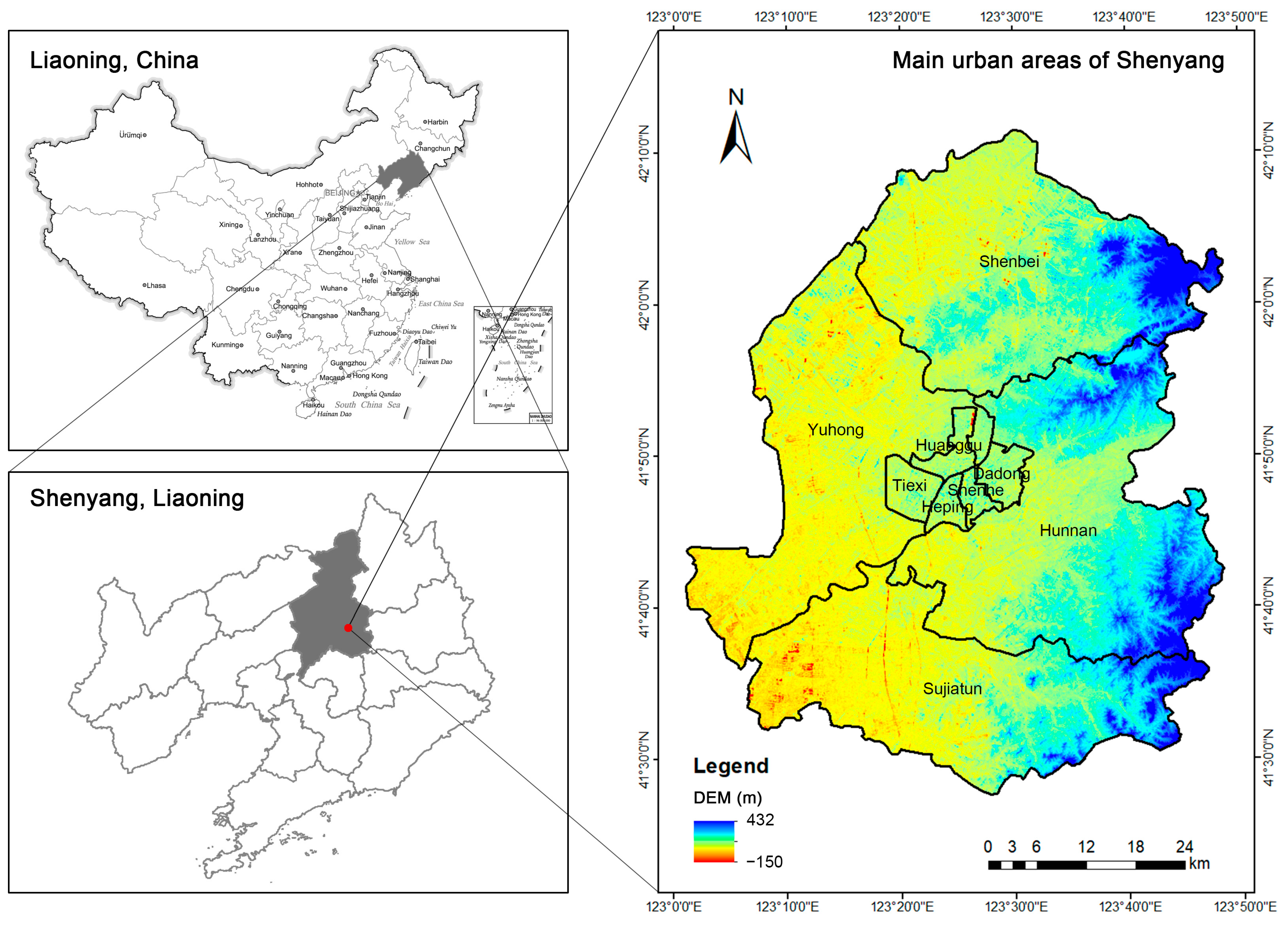
Shenyang is located at 41.20°~43.04°N and 122.42°~123.81°E, with a total area of about 12,860 square kilometers. Shenyang is the capital of Liaoning Province, China, and a typical city in cold regions. The terrain of Shenyang inclines from northeast to southwest, forming mountains, hills and alluvial plains. There are 27 rivers flowing through Shenyang, all belonging to the two major water systems, the Liao River and the Hun River. The Köppen climate classification classifies Shenyang as Dwa, i.e., cold and dry winters and hot and rainy summers. As the central city of Northeast China, Shenyang has developed rapidly in the last forty years. In 2020, the city had a resident population of 9.07 million and an urbanization rate of 84.52%, having reached an advanced stage of urbanization. As shown in Figure 1, the current study focuses on nine major municipal districts in Shenyang, namely, Heping District, Shenhe District, Dandong District, Huanggu District, Tiexi District, Sujiatun District, Hunnan District, Shenbei New District and Yuhong District, with a total study area of about 3766.76 square kilometers.
2.2. Data Sources and Preprocessing
This study acquired Landsat 5 TM images with a strip number of 119 and a shape number of 31 for 31 July 2000 and 12 August 2010 and Landsat 8 OLI images with a strip number of 119 and a shape number of 31 for 22 July 2020 from the Geospatial Data Cloud (http://www.gscloud.cn/search, accessed on 14 April 2022). All images with no or few clouds (less than 5%) in Shenyang were obtained in the summer, because the vegetation usually reaches its maximum growth in this season. The images were preprocessed using ENVI 5.3, with preprocessing including radiometric calibration, atmospheric correction and image cutting, to facilitate the calculation of LST and landscape composition indices.
Land cover data were obtained from Globeland30 (http://globeland30.org/, accessed on 14 April 2022). Compared to Globcover data with 300 m resolution and MODIS data with 500 m resolution, Globeland30 has a finer scale and is considered suitable for studies in developing countries [46]. Using Globeland30, the land cover categories in Shenyang were extracted and classified into six types: cropland, forest, grassland, wetland, water and impervious surface.
Worldpop (https://www.worldpop.org/, accessed on 14 April 2022) provided population density data for the years 2000 to 2020 at a spatial resolution of 1 km. Nighttime light data for 2000, 2010 and 2020 can be retrieved from the National Tibetan Plateau Data Center (http://data.tpdc.ac.cn, accessed on 14 April 2022) with a spatial resolution of 1 km. This dataset is the result of a nighttime light convolutional long short-term memory (NTLSTM) network. By applying the network, the researchers produced the world’s first 1984–2020 Chinese prolonged artificial nighttime light dataset [47]. Model evaluation against the original images showed a root-mean-square error (RMSE) of 0.73, a coefficient of determination (R2) of 0.95 and a linear slope of 0.99 at the pixel level, indicating the high quality of data for the generated product. The correlation between nighttime light data and socioeconomic indicators such as the built-up area, GDP and population at different stages is better than all existing products, validating the temporal consistency of this data product [47].
2.3. Methodology
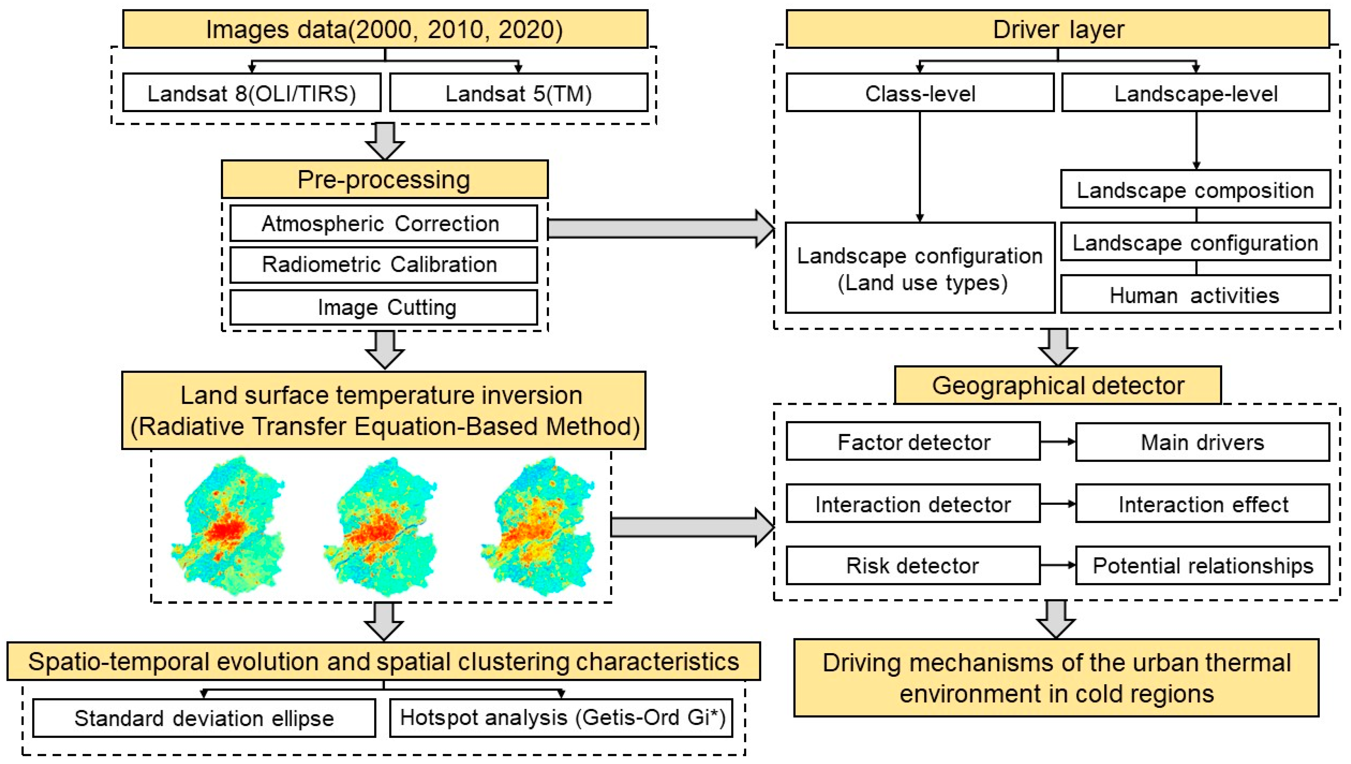
Our research consisted of four main steps: (1) the radiative transfer equation-based method (RTE) was used to obtain LSTs from 2000 to 2020; (2) spatial and temporal differentiation characteristics based on the multi-year LST dataset were analyzed; (3) the role of landscape configuration in LST for different land types in 2000, 2010 and 2020 was quantified using the geographical detector; (4) at the landscape level, the role of landscape composition, landscape configuration and human activities in LST in 2000, 2010 and 2020 was quantified using the geographical detector. The study flow chart is shown in Figure 2.
2.3.1. Land Surface Temperature Inversion
Based on band 6 of Landsat 5 TM in 2000 and 2010 and band 10 of Landsat 8 OLI in 2020, this study used the RTE for the inversion of LST. The RTE has been considered to have high accuracy in previous studies and has been widely used for the inversion of LST [48,49]. A simplified radiative transfer equation can express the brightness value of thermal infrared radiation:
where is the surface-specific emissivity, is the blackbody thermal radiation luminance, is the atmospheric transmittance in the thermal infrared band, is the atmospheric downward radiance, and is the atmospheric upward radiance. can be obtained as a function of Planck’s equation:
For band 6 of Landsat 5 TM, = 607.76 W/(m2∗µm∗sr) and = 1260.56 K. For band 10 of Landsat 8 OLI, = 774.89 W/(m2∗µm∗sr) and = 1321.08 K.
2.3.2. Acquisition of Independent Variables
As shown in Table 1, the findings of the researchers and the basic information about the study area led to the selection of three types of independent variables to examine the driving mechanism of the UTE.
Landscape composition indices mainly consist of biophysical components such as vegetation, water and built-up land. Based on previous studies, we quantified the landscape composition indices using FVC, NDBI and MNDWI.
The proportion of pixels containing the vertical projection of vegetation is called FVC. Previous studies have mostly used it to quantify the ecological status of the research area. Firstly, we obtained the using the following equation:
where is the near-infrared band, and is the red band.
Based on the results of , a dimidiate pixel model was used to obtain FVC, and 5–95% was selected as the confidence interval for the NDVI value. The formula is as follows:
where is the value of the fully vegetated area, and is the value of the non-vegetated area.
The NDBI is widely used to extract the construction sites in areas of interest. The calculation formula is as follows:
where is the mid-infrared band, and is the near-infrared band.
Compared to the NDWI, the MNDWI proposed by Xu [50] can effectively eliminate construction noise and consequently provide more accurate information on water body changes. The MNDWI is therefore often used to obtain water information from water areas where the background is dominated by built-up land. The is calculated as follows:
where is the green band.
Human activity indices were represented by preprocessed population density data and nighttime light data. Landscape configuration indices were quantified through landscape pattern indices, which were calculated based on land use data. Based on previous studies [16,38], seven landscape pattern indices were considered appropriate to quantify the landscape configuration at the class level and landscape level (Table 2). Five class-level indices were chosen to explore the landscape configuration of land cover; they represent the area factor, shape factor and aggregation factor. Additionally, six landscape-level indices were used to assess the structure and morphology of the entire landscape. In addition to the area factor, shape factor and aggregation factor, a diversity factor was added to the landscape-level indices. The landscape pattern indices were all calculated using Fragstats 4.0.
2.3.3. Standard Deviation Ellipse
The SDE introduced by Lefever [51] was used to spatially quantify the distribution characteristics of and spatio-temporal variation in the study object. The basic characteristics of the SDE include the long axis, short axis, shape and range. The long and short axes indicate the direction and extent of the spatial distribution of the study object, respectively. The higher their ratio, the more concentrated and directional the study object is. Conversely, the lower the ratio, the more discrete and less directional the study object is. In addition, the gravity center can be used to assess the trend of a geographical object over time [52]. By comparing changes in the gravity centers of the ellipses at different times, the development trend and trajectory changes in the study object can be estimated spatially. This study used the SDE to determine the migration trajectory of the hotspot regions of LST.
2.3.4. Hotspot Analysis (Getis–Ord Gi*)
The hotspot analysis method proposed by Ord and Getis [53] is an effective method for studying the spatial clustering characteristics of research objects. By calculating the z-scores and p-values of elements, the method can effectively explore where the clustering of high- or low-value elements occurs in space. Elements with high values and surrounded by other elements having high values are usually statistically significant hotspots. We performed the hotspot analysis of LST using the hotspot analysis tool of Arc GIS 10.4.1. The results obtained with this tool can show the spatial clustering of cold and hotspots in LST.
2.3.5. Geographical Detector
As a statistical tool for measuring spatial heterogeneity, the geographical detector has been widely used in recent years [37]. This tool can effectively measure the relationship between variables and identify the explanatory variables that contribute primarily to the spatial heterogeneity of the dependent variable, without assuming the linearity of the association between them [36]. The geographical detector consists of four parts: a factor detector, risk detector, ecological detector and interaction detector. In this study, the direct effect of selected drivers on the spatial heterogeneity of LST was analyzed using the factor detector. The results can be expressed as q-statistics:
where L is the number of strata of explanatory variables (h = 1, 2, …, L), N is the number of samples, and stratum h consists of units. is the variance of the dependent variable, and represents the variance in the dependent variable in stratum h.
The value of q ranges within [0, 1]. The closer the value of q is to 1, the stronger the explanatory power of the explanatory variable, and the closer it is to 0, the weaker the explanatory power.
The risk detector was used to identify significant differences between the means of the dependent variable and the explanatory variable in the two sub-regions, which in turn determined the potential risk region of the dependent variable. The interaction detector determined whether the explanatory power of two explanatory variables superimposed on each other was enhanced, diminished or mutually independent.
Since the explanatory variables of the geographical detector need to be discretized, the Jenks natural breaks classification method was used to classify the means of independent variables into nine classes and incorporate them into 967 2 km × 2 km grids for calculation. Major urban blocks in China are rectangles of approximately 800 m to 1200 m in length, so grid cells of 1 km to 5 km are suitable for urban-scale studies [54]. In previous studies, a grid scale of 2 km × 2 km has been considered the best scale for exploring the driving mechanisms of LST [55]. Therefore, a 2 km × 2 km analysis unit was chosen to explore the driving mechanism of LST in this study.
3. Results
3.1. Validation of LST Results
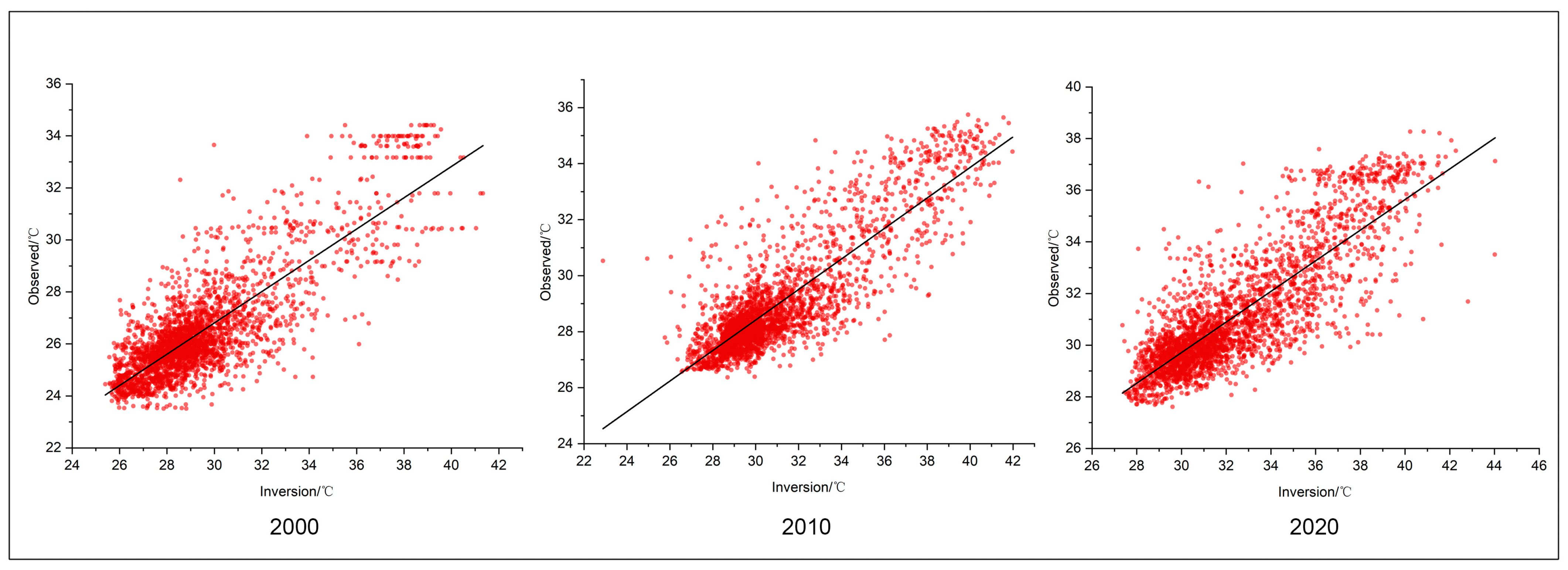
We validated the LST results for 2000, 2010 and 2020 using the MOD11A1 Version 6.1 product (MODIS/Terra Land Surface Temperature/Emissivity Daily L3 Global 1 km SIN Grid) obtained from LAADS DAAC (https://ladsweb.modaps.eosdis.nasa.gov/, accessed on 24 March 2023). The product provides daily per-pixel LST and emissivity with a spatial resolution of 1 km [56]. Previous studies have demonstrated that this product can be used to validate LST results [57].
MOD11A1 1 km LST data on the same date as the selected Landsat remote-sensing images for this study were extracted as validation data. Afterward, linear fits were made using these data and inverse Shenyang LST data to verify the accuracy of LST in this study. Figure 3 shows the results of linear fitting. The Pearson correlation coefficients were 0.825, 0.852 and 0.829, with a root-mean-square error (RMSE) of 1.173, 2.728 and 2.247 in 2000, 2010 and 2020, respectively. This indicates that the inverse LST and validation data in this study are well correlated and suitable for use in subsequent studies.
3.2. Spatial and Temporal Differences in LST
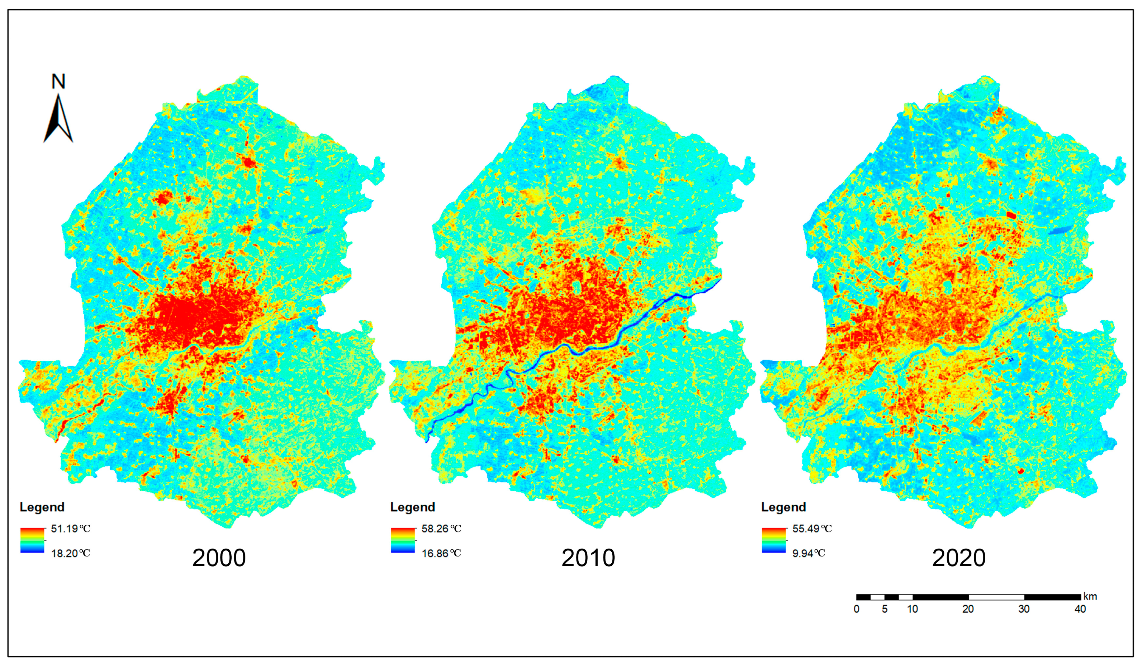
Figure 4 shows the spatial distribution of and temporal changes in LST in Shenyang from 2000 to 2020. Over 20 years, the area of Shenyang’s high-temperature region continued to expand. The average LSTs of Shenyang were 29.49 °C, 31.08 °C and 32.47 °C in 2000, 2010 and 2020, respectively, exhibiting an increasing trend, according to Table 3. The temperature difference was growing in 2000, 2010 and 2020, with values of 32.99 °C, 41.40 °C and 45.55 °C. In addition, the standard deviation (SD) of the mean LST also widened, with 3.37, 3.69 and 3.85 in the three periods, respectively. These results indicate that LST in Shenyang tends to deteriorate, which is accompanied by a significant increase in heterogeneity.
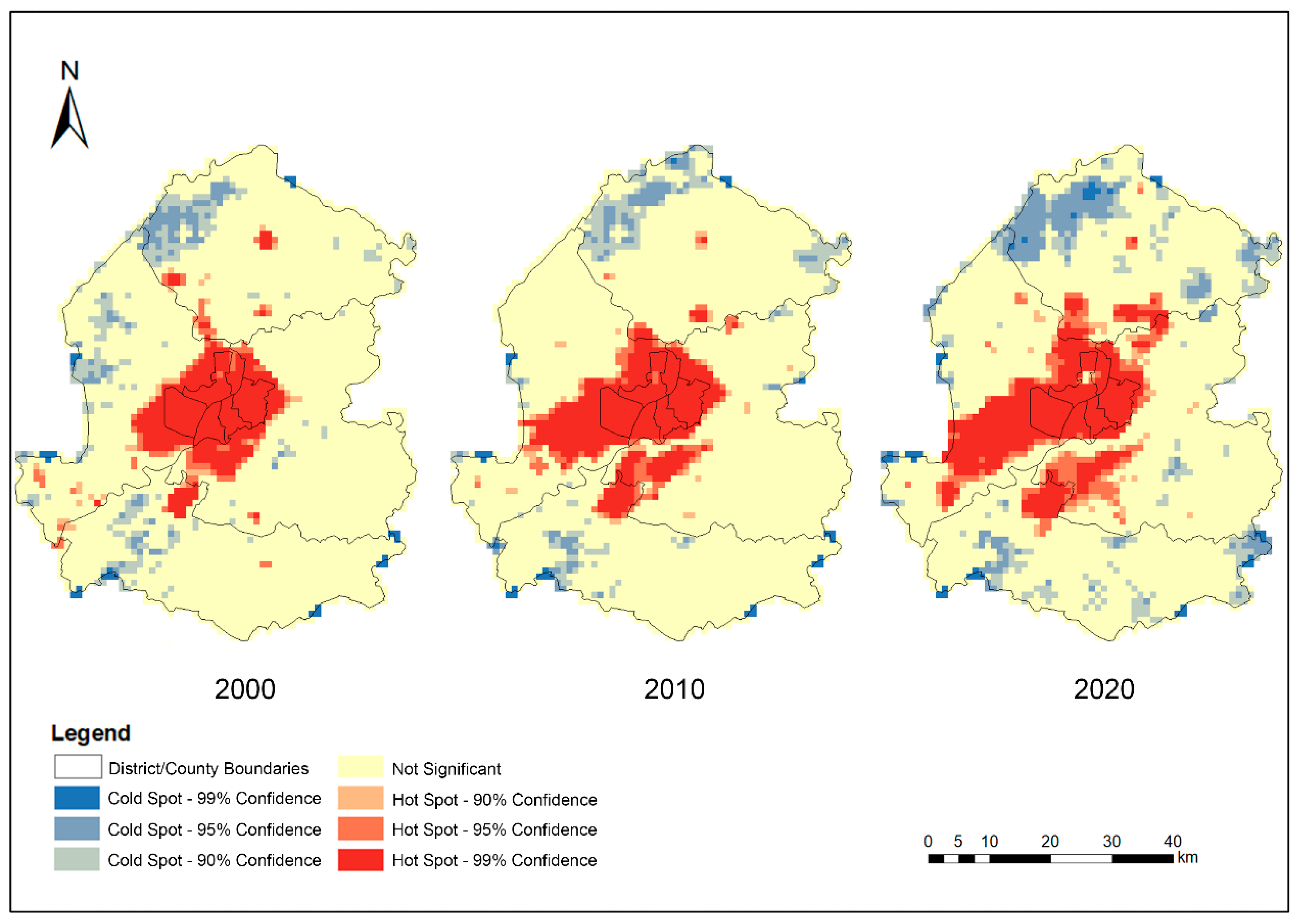
The results of the hotspot analysis (Getis–Ord Gi*) show the spatial clustering characteristics of LST in 2000, 2010 and 2020 (see Figure 5). Overall, the central urban area always contained hotspots, while the suburban area near water and vegetation contained most of the cold spots. Over a period of 20 years, the clustering areas of hot and cold spots tended to expand. In 2000, the regions described as hot and cold spots accounted for 12.67% and 9%, respectively; in 2010, they were 15.4% and 7.85%, respectively; and in 2020, they were 19.22% and 13.57%, respectively (see Figure 6). In addition, the hotspots formed by the Hun River and its surrounding areas in the central urban area have gradually disappeared, resulting in the gradual separation of hotspots in the central urban area along the Hun River over a period of 20 years and the formation of two separate heat islands across the north and south banks of the Hun River.
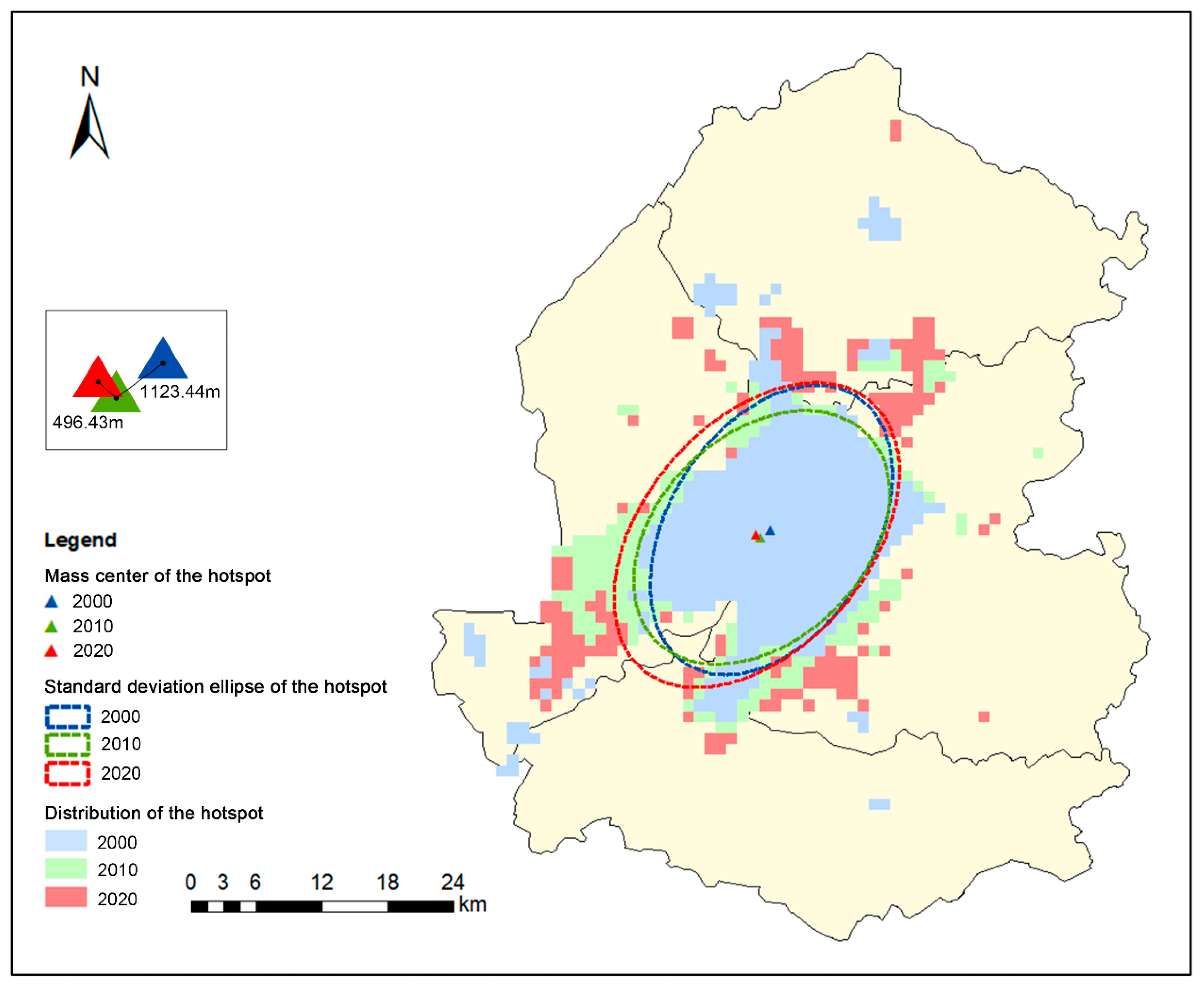
Figure 7 shows the expansion patterns of the hotspot areas acquired using the SDE. The gravity center of the ellipse was always in the center of Shenyang, near the border of Tiexi and Heping Districts. From 2000 to 2010, the gravity center shifted 1123.44 m to the southwest, while in the following decade, it shifted 496.43 m to the northwest. The rotation angle of the ellipse can reflect the development direction of the hotspot regions, as shown in Table 4. From 2000 to 2010, the rotation angle of the ellipse increased clockwise from 32.38 degrees to 45.96 degrees. Then, from 2010 to 2020, the rotation angle decreased counterclockwise from 45.96 degrees to 40.58 degrees. These rotations indicate that the direction of the hotspot was altered over the 20-year period and elongated in the northeast–southwest direction. The ratio of the long axis to the short axis expresses the spatial dispersion of the hotspot regions. From 2000 to 2020, the ratio first decreased and then increased, showing the development trend of hotspot regions from dispersion to concentration.
LSTs for different land types also show significant variations (Table 5). Over the 20-year period, the mean values of LST increased significantly for all land use types. The impervious surface was consistently the hottest land use type, with mean LST values of 33.69 °C, 35.75 °C and 36.80 °C in the three periods, respectively. The mean LST for forests in 2000 was 28.06 °C, making it the coldest land use type. However, in 2010 and 2020, it was replaced by water, with mean LSTs of 26.49 °C and 29.74 °C, respectively. This confirms that natural surfaces covered by water and forests can effectively reduce the ambient temperature.
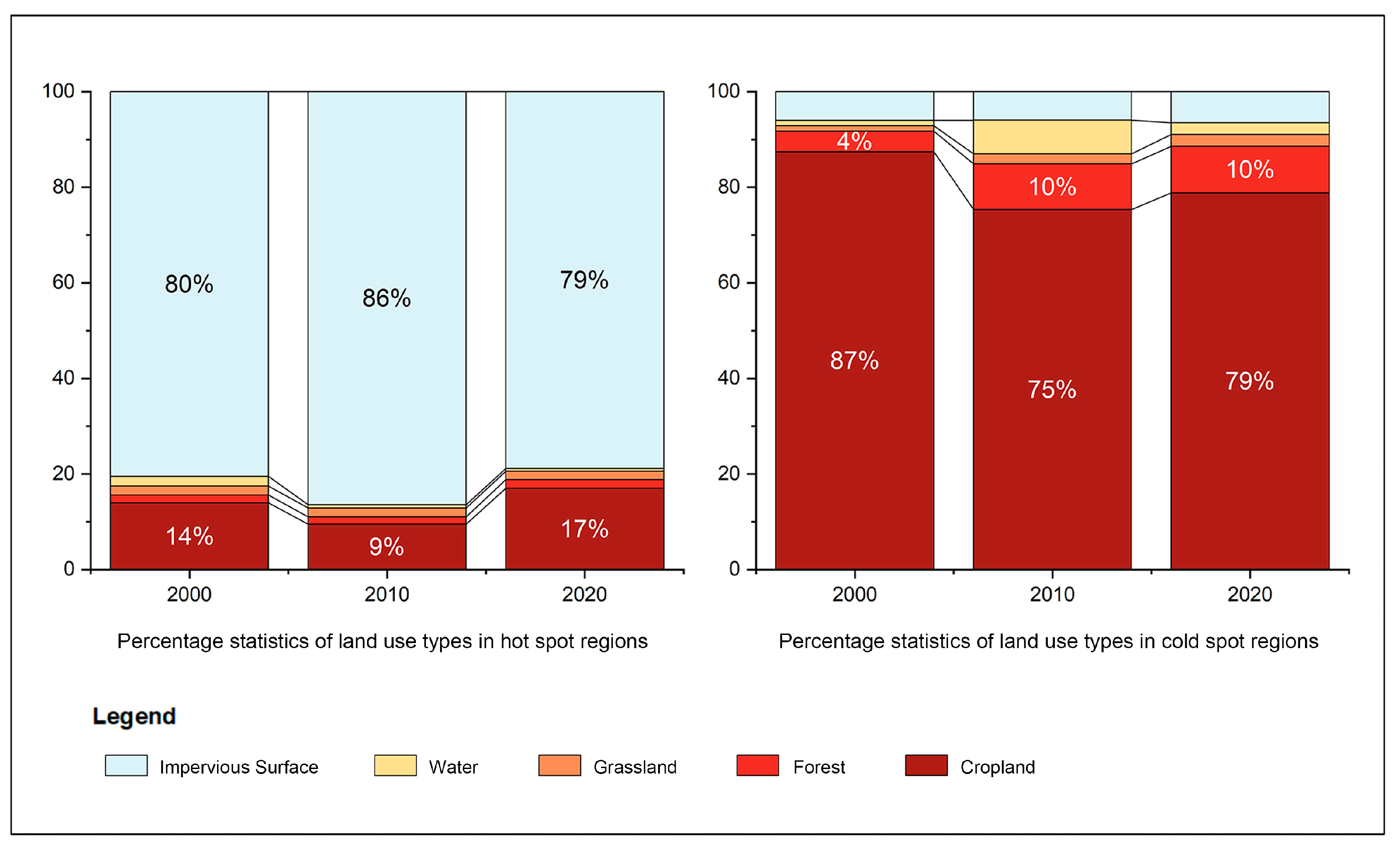
Figure 8 shows the results of superimposed hotspot analysis and land use types. Over 75% of the cold spot regions were concentrated in croplands near water bodies over the 20-year period. In addition, more than 79% of the hotspot regions were covered by impervious surfaces. It can be inferred that the construction land in the urban core of Shenyang leads to the aggregation of hotspots of LST. Conversely, large areas of cropland on the outskirts of the city lead to the clustering of cold spots.
3.3. The Driving Mechanism of LST
3.3.1. Factor Detection Analysis
Since only one delineated grid contained wetland, it was difficult to quantify the effect on the heterogeneity of LST. In the subsequent analysis, wetland was excluded. The analysis results of class-level factor detection are shown in Table 6. Over the 20 years, some landscape configuration indices of cropland, water and impervious surface significantly influenced the spatial differentiation of LST (p < 0.1). The explanatory power of PLAND and LPI for the LST of impervious surfaces was consistently above 51%, while that for the LST of cropland was consistently above 27%. This means that the area factor of cropland and impervious surface is critical to LST heterogeneity. The explanatory power of FRAC_AM for the LST of impervious surfaces was 18% in 2000 and 20% in 2010, respectively. However, by 2020, it had dropped to 11% and was no longer significant. This may imply that the shape factor of the impervious surface has a reduced driving force on LST. Moreover, in 2010, the explanatory power of LPI and FRAC_AM for the LST of water was 37% and 16%, respectively, indicating that the area factor and shape factor of water may also affect LST.
Table 7 shows the results of factor detection at the landscape level. Under the premise that significance was always satisfied, the average factor explanatory power at the landscape level was as follows: NDBI > FVC > nighttime light > population density > MNDWI > FRAC_AM. Among all the landscape configuration indices, only FRAC_AM had an explanatory power that was always greater than 10% and was always significant. In contrast, other factors had weaker explanatory power (less than 10% or not significant) for the heterogeneity of LST. Overall, the landscape composition indices and the human activity indices are more important for LST heterogeneity, with an average explanatory power greater than 40%, while the landscape configuration indices are secondary drivers.
3.3.2. Risk Detection Analysis
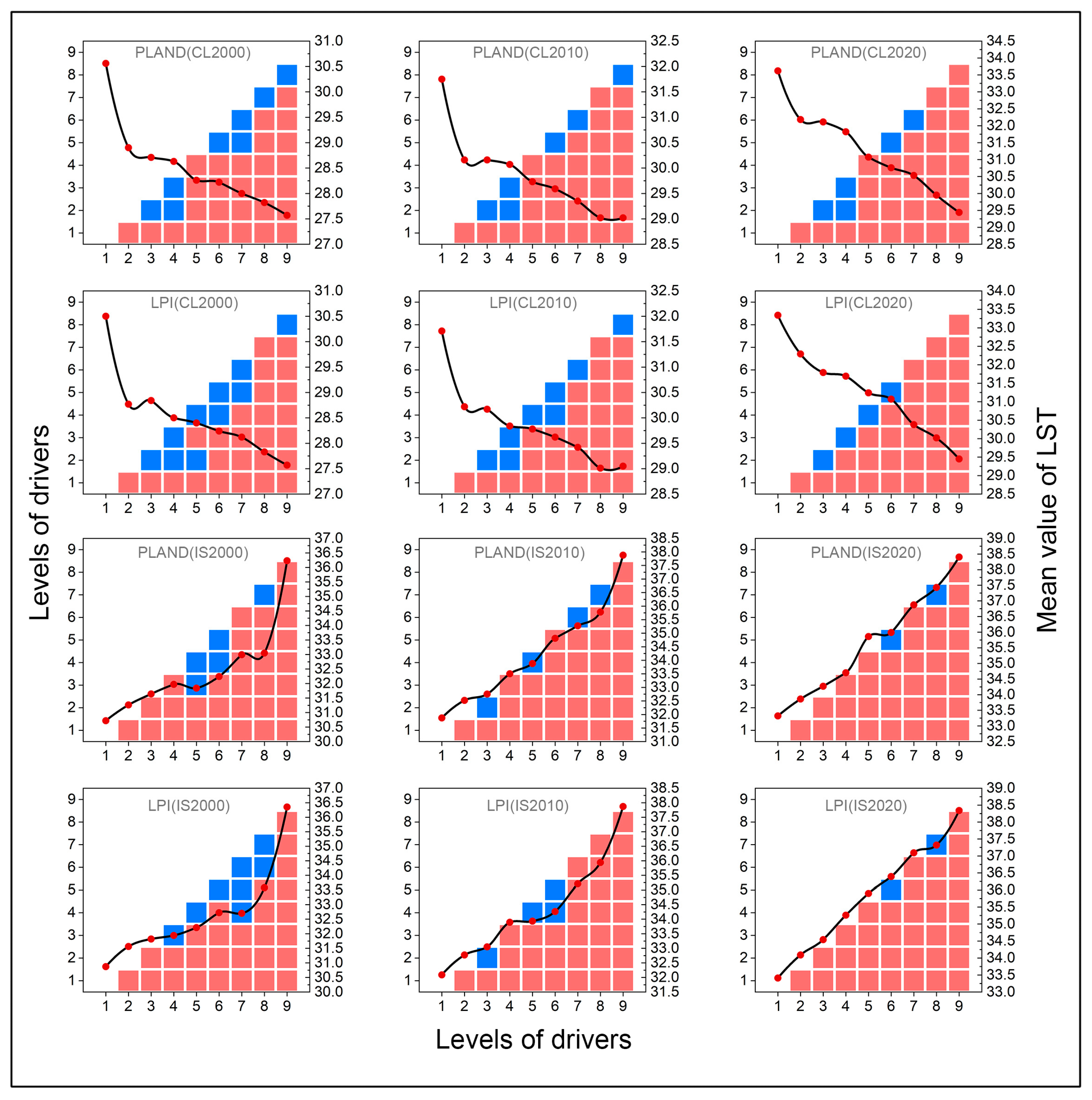
The drivers that were significant contributors to LST heterogeneity over 20 years were selected for risk detection analysis. Figure 9 presents the results of class-level risk detection. The LST of cropland decreased with increasing PLAND and LPI, while the opposite was true for that of impervious surfaces. In addition, the LST of cropland varied considerably in the first two classes of PLAND and LPI. The LST of impervious surfaces, in contrast, increased rapidly in the latter two classes of PLAND and LPI. However, these differences diminished over time for cropland and impervious surfaces.
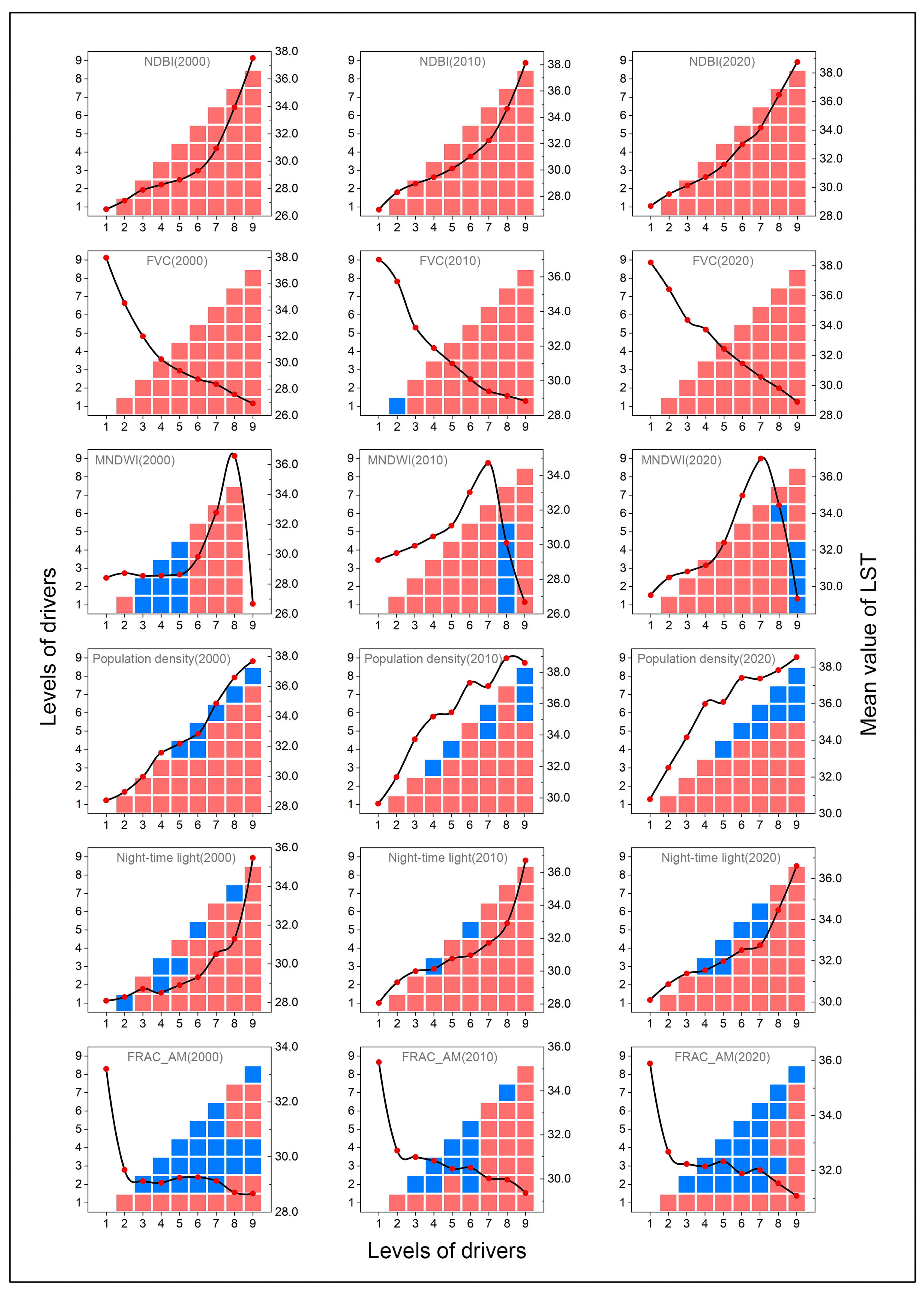
In the landscape-level risk detection analysis, the relationship between different drivers and LST differs significantly (Figure 10). The NDBI, population density and nighttime light were positively correlated with LST, which means that the development of construction land, the growth of the population and the increase in the socioeconomic level will increase LST. Compared to the NDBI, population density and nighttime light, FVC had a near-linear negative association with LST. For FRAC_AM, LST always decreased rapidly in the first two levels and showed a constant negative correlation in the subsequent levels. In addition, the MNDWI was found to show a significant nonlinear association with LST. LST increased rapidly with increasing levels of MNDWI, peaking between levels 7 and 8. At subsequent levels, LST decreased rapidly.
3.3.3. Interaction Detection Analysis
Figure 11 and Figure 12 show the results of interaction detection at the class level and the landscape level, respectively. The q-values of the interactions between different drivers all showed bidirectional enhancement or nonlinear enhancement (dark underline). Bidirectional enhancement means that the effect of the interaction between drivers is stronger than their individual effects, while nonlinear enhancement means that the interaction between drivers exceeds the sum of their individual effects. That is, in the present study, the superposition of any two drivers enhances their effects on the heterogeneity of LST.
At the class level, LPI∩ED (61%), PLAND∩ED (65%) and PLAND∩FRAC_AM (58%) for impervious surfaces had the strongest interactions in 2000, 2010 and 2020, respectively. LPI∩ED (37%), PLAND∩ED (41%) and PLAND∩ED (43%) for cropland also showed strong interactions in 2000, 2010 and 2020, respectively. It was also found that LPI∩FRAC_AM for water had 52% and 33% of the interaction in 2010 and 2020, respectively. PD, ED and FRAC_AM had weaker explanatory power in single-factor detection, but their explanatory power for LST heterogeneity could be significantly enhanced when combined with other factors.
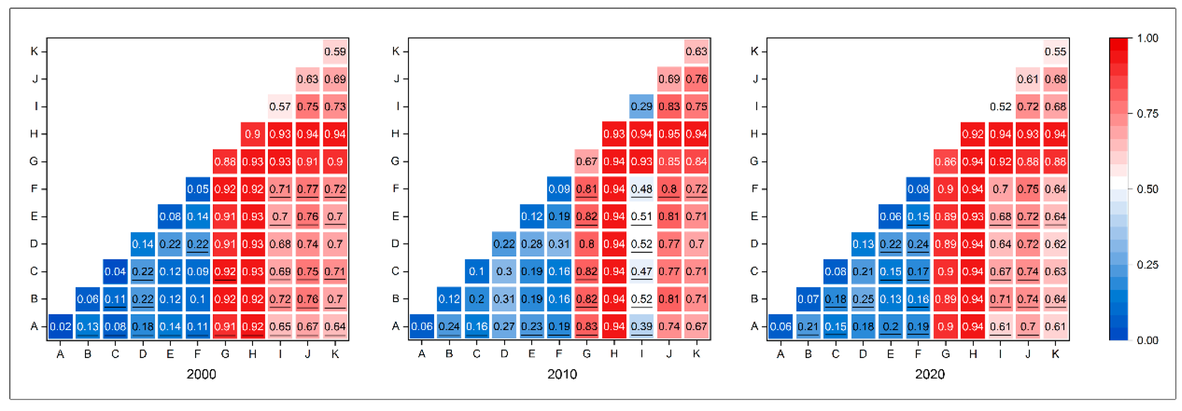
Among the landscape-level interactions, the NDBI was the main contributor to LST heterogeneity at different times. In 2000, NDBI ∩nighttime light and NDBI ∩population density had the strongest interactions on LST heterogeneity. In 2010, NDBI ∩nighttime light and NDBI ∩FVC had the highest contribution to LST heterogeneity. Finally, NDBI ∩FVC and NDBI ∩SHDI had the strongest interaction effects on LST heterogeneity in 2020. The explanatory variables that possess the strongest interactions at the landscape level involve all three categories, implying that the interactions among landscape composition indices, landscape configuration indices and human activity indices have a significant effect on the spatial differentiation of LST.
4. Discussion
4.1. Spatial and Temporal Differences
Researchers in urban ecology believe that the UTE reflects the result of the surface and atmospheric energy balance [11]. The study of the spatial and temporal differentiation of the UTE is fundamental to understanding ecological change and urban development [12,31]. From 2000 to 2020, LST in Shenyang continued to rise. The hotspots consistently extended in the northeast–southwest direction, and the hot/cold spots in the city center and its suburbs kept expanding. These findings indicate that rapid urbanization has indeed resulted in the deterioration and spatial heterogeneity of the UTE [58].
Among all land use types, we found that the hotspot regions were always concentrated on impervious surfaces. Impervious surfaces, including impervious landscapes and exposed surfaces in cities, are thought to always increase urban temperatures by holding heat and reducing evaporative cooling [59]. It is noteworthy that, although water and forest were always the land types with the lowest mean values of LST, the cold spots in Shenyang were always clustered in croplands near water during the 20 years. This may be influenced by the area of land cover [60]. As shown in Table 8, cropland was always the dominant land type in the study area, with a consistent percentage of over 58%, although it continued to decrease. In contrast, forest and water continued to expand, but the sum of the areas never exceeded 9%. For the whole study area, the smaller area proportions make it difficult to form spatial clusters with significant cold spots in forest and water. However, the growth of large areas of crops in summer, such as corn and rice, can lead to an increase in surface soil moisture and evapotranspiration and thus can promote the clustering of cold spots [61,62].
An interesting phenomenon is that the LST hotspots in the Hun River and its surrounding areas in the central city of Shenyang have been disappearing over the past 20 years, creating two heat islands to the north and south along the Hun River. This may be due to the pollution control and ecological protection of the Hun River. As an important industrial city in China, Shenyang has well-developed food and chemical industries, but the uncontrolled discharge of pollutants led to extremely serious pollution of the river until 2002 [63]. The Shenyang municipal government then embarked on river management and gradually established the landscape corridor to optimize the quality of the river and its surrounding ecology [63]. Through these measures, the LST in the area has also been reduced, gradually creating a corridor separating LST hotspots.
4.2. Driving Mechanism at the Class Level
The relationship between the landscape configuration and LST varies considerably across land types at the class level. On longer time scales, the PLAND and LPI of cropland and impervious surfaces were always the main landscape configuration indices that affected LST. The intensity of LST decreases as the area and patches of cropland increase, while the opposite is true for impervious surfaces. As part of the urban green space, the positive impact of the increased size and abundance of cropland on LST is associated with increased irrigation and an increased scale of transpiration during crop growth peaks [64,65]. Furthermore, the aggregation and large-scale expansion of built-up land can lead to a reduction in surface infiltration and surface moisture, which in turn leads to the deterioration of LST [66].
It is noteworthy that the LST of cropland always decreased rapidly in the first two levels of LPI and PLAND, and the LST of impervious surfaces always increased rapidly in the last two levels of LPI and PLAND. This implies that the transpiration cooling effect of cropland on LST occurs rapidly with increasing area and abundance [67]. Moreover, when the impervious surface increases to a certain extent, unrestricted urban expansion leads to difficulties in finding a balance between urban development and urban ecology, resulting in a rapid rise in LST [68]. However, over the 20-year period, the difference in LST increased for each level of PLAND and LPI, and the relationship between PLAND, LPI and LST gradually changed from nonlinear to near-linear. This can be attributed to rapid urbanization [69]. Rapid urbanization has led to massive urban expansion, rapid land cover changes and ever-increasing LST. In this case, while the PLAND and LPI of cropland and impervious surfaces still have effects on LST, their marginal effects are more difficult to specify, and further attention needs to be paid to the interaction of landscape configuration to maximize LST reduction.
For other landscape configuration indices, even if the individual explanatory power was not strong, the interactions between them tended to enhance their impact on LST. This implies that the complex synergy of factors is more important than the role of a single factor [38]. The strongest explanatory power of the interactions appeared in the area and shape indices of the impervious surface, including LPI, PLAND, ED and FRAC_AM. This suggests that the combination of area, abundance, shape and connectivity patterns of different patches of impervious surface needs to be focused on when optimizing the UTE [70]. The PLAND, LPI and ED of cropland also showed strong interactions, suggesting that the combined configuration of the area, abundance and patch connectivity patterns of cropland also needs to be taken into account. Attention also needs to be paid to the interacting configurations of the LPI and FRAC_AM of water, as they also showed stronger interactions in 2010 and 2020.
4.3. Driving Mechanism at the Landscape Level
Landscape composition and human activities are key drivers that influence LST at the landscape level. The NDBI, population density, and nighttime light were significantly and positively correlated with LST from 2000 to 2020. During the rapid expansion phase of cities, population migration and economic activity can increase anthropogenic heat release and LST [71,72]. In contrast, FVC showed a significantly negative correlation with LST. Urban green areas can promote air ventilation by improving the thermodynamic properties of the land surface, which can help reduce LST in urban areas [71,73]. Unlike previous studies, the MNDWI and LST were not always significantly negatively correlated, but rather, there was a threshold effect. The positive effect of the MNDWI on LST could be attributed to the fact that the remote-sensing images were acquired at night and in late summer. Gunawardena et al. [74] showed that urban heat island intensity is greatest at night and in late summer, which may lead to warming effects on water bodies. In addition, we speculate that LST will rapidly decrease when the surface water content reaches a certain threshold.
The landscape configuration indices had less explanatory power for LST at the landscape level than at the class level. This finding might further indicate that the configuration of land cover is more valuable than that of the entire landscape when studying the driving forces of LST [75,76]. However, we still found strong explanatory power for FRAC_AM for LST at the landscape level. Complex landscape patches can lead to a reduction in LST, especially in the first two levels of FRAC_AM. Zhao et al. [27] argued that the shape complexity of urban landscapes should receive more attention when aiming to reduce the LST of cities, which is consistent with our findings.
With the exception of the MNDWI and FRAC_AM, all drivers showed a near-linear correlation trend with LST over 20 years, similar to the results at the class level. This suggests that more attention also needs to be paid to the interaction of drivers at the landscape level during the rapid urbanization phase.
The two variables with the strongest interaction effects on LST were constantly changing over 20 years. However, one of the interacting variables always included the NDBI. The single explanatory power of the NDBI for LST is very strong, but the explanatory power can still be enhanced by its interaction with other factors, such as nighttime lighting, population density, FVC and SHDI. These findings emphasize the importance of built-up areas in LST at the landscape level. At the same time, urban planners need to pay attention to the combination of buildings and vegetation, population, economic activity and the diversity of the landscape when optimizing the UTE.
4.4. Impact on Urban Planning
This study explored the spatial and temporal differentiation characteristics and driving mechanisms of the UTE. In addition, the differences in driving mechanisms across different stages of urbanization were investigated. The results of this study may therefore have important implications for UTE-based urban planning. At the landscape level, due to the high correlation between the NDBI, population density and nighttime light and LST, the high density of buildings, concentrated population and frequent economic activities can have a significant impact on UTE deterioration. Therefore, urban sprawl and human activities should first be strictly controlled during rapid urbanization. FVC and FRAC_AM are significantly negatively correlated with LST, so during rapid urbanization, increasing vegetation cover and landscape diversity can help to rapidly optimize the UTE, for example, by creating pocket parks and landscape corridors in high-density urban cores and increasing the protection of ecological reserves in the outskirts of cities. The marginal contribution of the MNDWI to LST suggests that the stock of water bodies should be maintained, their quality should be improved, and large lakes should be built on the outskirts of the city. At the class level, the relationship between PLAND and LPI and LST for cropland and impervious surfaces indicates that an ecological red line for cropland should be drawn, and continuous cropland should be built on the outskirts of the city to avoid the encroachment on cropland caused by concentrated urban development during rapid urbanization. The integration of the main drivers at the landscape level and class level allows for the efficient optimization of the UTE during rapid urbanization.
In the later stage of rapid urbanization, the development of large urban areas is constrained, and the marginal contribution of a single driver to UTE is reduced. At this stage, therefore, urban planners need to focus on the interactions between drivers to maximize the reduction in LST. Firstly, according to our study, the combination of the area, abundance, shape and patchy connectivity patterns of impervious surfaces needs to be focused on. This means that when controlling urban sprawl, attention should also be paid to the diversity of morphology and the complexity of the boundaries of urban built-up areas. Secondly, the area, abundance and patch connectivity patterns of cropland have strong effects on LST. This suggests that when conserving cropland, attention needs to be paid to the size of the cropland, the type of crop and the complexity of the cropland boundaries. Thirdly, the abundance and morphology of water can also significantly interact with LST, and it is therefore recommended that when increasing water area, it should be combined with a diversity of morphological features. Finally, the combination of buildings and vegetation, population, economic activity and landscape diversity has a significant impact on LST, suggesting that, in the later stage of rapid urbanization, urban development should be intensified, and the ecological benefits of the landscape should be achieved by allocating diverse vegetation and landscape functions to high-density built-up areas.
5. Conclusions
Based on three Landsat images of Shenyang city in 2000, 2010 and 2020, we investigated the spatial and temporal differentiation characteristics of the UTE and its driving mechanisms during rapid urbanization using the SDE, hotspot analysis and the geographical detector. We identified the driving mechanisms by which landscape composition, landscape configuration and human activities affect the UTE at multiple levels. The key findings of this study are as follows.
Firstly, the average LST in Shenyang continued to rise and had significant spatial and temporal differentiation characteristics during the twenty-year period. The hotspot regions extended in the northeast–southwest direction. Hotspot and cold spot areas continued to expand in urban and suburban areas, respectively. The hotspots were always concentrated on impervious surfaces, while the cold spots were scattered in croplands near water. Over a period of 20 years, the hotspot in the central city has gradually been divided into two parts along the north and south banks of the Hun River.
Secondly, the spatial configuration indices at the class level are more important than those at the landscape level when studying the UTE. PLAND and LPI for class-level cropland and impervious surfaces were strong drivers of LST over the 20-year period, whereas only FRAC_AM at the landscape level had a consistently significant effect on LST.
Thirdly, as urbanization progresses, the marginal effects of some drivers on LST decrease, showing a near-linear correlation. At the class level, increases in the PLAND and LPI of cropland could rapidly reduce LST, while increases in the PLAND and LPI of impervious surfaces could rapidly increase LST. At the landscape level, the NDBI, population density and nighttime light were positively correlated with LST, FVC and FRAC_AM could effectively reduce LST, and there was a threshold for the response of the MNDWI to LST. However, over a period of 20 years, the nonlinear relationship between all factors and LST, except the MNDWI and FRAC_AM, gradually shifted to a near-linear relationship.
Finally, the interaction between the drivers should receive more attention when optimizing the UTE in the later stage of rapid urbanization. All class-level and landscape-level factors had enhanced effects on LST through their interactions. At the class level, the focus needs to be on the combination of the area, abundance, shape and patch connectivity patterns of impervious surfaces. The combined configuration of the area, abundance and patch connectivity patterns of cropland and the patch abundance and shape of water also need to be considered. At the landscape level, attention needs to be paid to the integration of buildings and vegetation, population, economic activity and landscape diversity. These results will provide the basis for a more comprehensive understanding of the UTE and the implementation of urban planning strategies during rapid urbanization.
Our study also has some limitations. First, our study was conducted only in Shenyang, a typical city in cold regions. The spatial pattern of LST may vary greatly among different cities due to differences in urban development patterns. Recent studies have concluded that conducting studies on LST in different cities or urban clusters can avoid bias in the results [13,77]. Second, in this study, only three remote-sensing images were selected for the time-scale research. Although the meteorological conditions of the selected remote-sensing images are similar and good, it is difficult to reflect the results of the study on a time scale of 20 years with data from only three remote-sensing images. Follow-up studies could increase the number of remote-sensing images to draw more precise conclusions. Third, we studied only one analysis unit at 2 km*2 km. Although this unit is recognized, the modifiable areal unit problem (MAUP) may exist, and different analysis scales may lead to differences in the results [54]. Therefore, in future UTE studies, the inclusion of different statistical scales should be considered to increase the accuracy of the results. Finally, the drivers affecting changes in the UTE may not be limited to two-dimensional composition and configuration. Three-dimensional landscape indicators, such as the floor area ratio and shadow patterns, have been found to influence the UTE [78,79]. However, this was not discussed in this study. The relationship between three-dimensional urban landscape metrics and the UTE should be emphasized and combined with two-dimensional metrics for a comprehensive analysis.
Author Contributions
Y.J.: Conceptualization, Methodology, Formal Analysis, Investigation, Writing—Original Draft and Writing—Review and Editing. Y.P.: Conceptualization, Supervision and Writing—Review and Editing. Z.L.: Software, Validation, Investigation and Visualization. J.L.: Data Curation and Investigation. S.L.: Conceptualization, Methodology, Project Administration, Funding Acquisition and Writing—Review and Editing. X.C.: Investigation and Funding Acquisition. Y.Y.: Investigation and Visualization. T.F.: Writing—Review and Editing. All authors have read and agreed to the published version of the manuscript.
Funding
This research was supported by the National Natural Science Foundation of China (grant numbers 42177072 and 52108049) and the Fundamental Research Funds for the Central Universities of Central South University (grant number 1053320212429). This research was also made possible by the Natural Science Foundation of Hunan Province, China (grant number 2020JJ4711), and the Humanities and Social Science Fund of Ministry of Education of China (grant number 20YJCZH003).
Data Availability Statement
The land cover data in 2000, 2010 and 2020 were obtained from Globeland 30 (http://globeland30.org/, accessed on 14 April 2022). The Landsat 5 TM images with a strip number of 119 and a shape number of 31 for 31 July 2000 and 12 August 2010 and Landsat 8 OLI images with a strip number of 119 and a shape number of 31 for 22 July 2020 were obtained from the Geospatial Data Cloud (http://www.gscloud.cn/search, accessed on 14 April 2022). The population density data in 2000, 2010 and 2020 were obtained from WorldPop (https://www.worldpop.org/, accessed on 14 April 2022). The nighttime light data in 2000, 2010 and 2020 were obtained from the National Tibetan Plateau Data Center (http://data.tpdc.ac.cn, accessed on 14 April 2022). The MOD11A1 Version 6.1 product (MODIS/Terra Land Surface Temperature/Emissivity Daily L3 Global 1km SIN Grid) was obtained from LAADS DAAC (https://ladsweb.modaps.eosdis.nasa.gov/, accessed on 24 March 2023).
Conflicts of Interest
The authors declare that they have no known competing financial interest or personal relationships that could have appeared to influence the work reported in this paper.
References
- Mirzaei, M.; Verrelst, J.; Arbabi, M.; Shaklabadi, Z.; Lotfizadeh, M. Urban Heat Island Monitoring and Impacts on Citizen’s General Health Status in Isfahan Metropolis: A Remote Sensing and Field Survey Approach. Remote Sens. 2020, 12, 1350. [Google Scholar] [CrossRef]
- Peng, Y.; Feng, T.; Timmermans, H.J. Heterogeneity in outdoor comfort assessment in urban public spaces. Sci. Total Environ. 2021, 790, 147941. [Google Scholar] [CrossRef] [PubMed]
- Yue, W.; Qiu, S.; Xu, H.; Xu, L.; Zhang, L. Polycentric urban development and urban thermal environment: A case of Hangzhou, China. Landsc. Urban Plan. 2019, 189, 58–70. [Google Scholar] [CrossRef]
- Chen, Y.; Yang, J.; Yang, R.; Xiao, X.; Xia, J. Contribution of urban functional zones to the spatial distribution of urban thermal environment. Build. Environ. 2022, 216, 109000. [Google Scholar] [CrossRef]
- IPCC. Climate Change 2021: The Physical Science Basis; IPCC: Geneva, Switzerland, 2021. [Google Scholar]
- Yu, Z.; Yao, Y.; Yang, G.; Wang, X.; Vejre, H. Strong contribution of rapid urbanization and urban agglomeration development to regional thermal environment dynamics and evolution. For. Ecol. Manag. 2019, 446, 214–225. [Google Scholar] [CrossRef]
- Aboelata, A.; Sodoudi, S. Evaluating urban vegetation scenarios to mitigate urban heat island and reduce buildings’ energy in dense built-up areas in Cairo. Build. Environ. 2019, 166, 106407. [Google Scholar] [CrossRef]
- Akande, O. Urbanization, Housing Quality and Health: Towards a Redirection for Housing Provision in Nigeria. J. Contemp. Urban Aff. 2020, 5, 35–46. [Google Scholar] [CrossRef]
- Caprotti, F.; Romanowicz, J. Thermal Eco-cities: Green Building and Urban Thermal Metabolism. Int. J. Urban Reg. Res. 2013, 37, 1949–1967. [Google Scholar] [CrossRef]
- Xie, Q.; Sun, Q. Monitoring thermal environment deterioration and its dynamic response to urban expansion in Wuhan, China. Urban Clim. 2021, 39, 100932. [Google Scholar] [CrossRef]
- Zhuang, Q.; Wu, S.; Yan, Y.; Niu, Y.; Yang, F.; Xie, C. Monitoring land surface thermal environments under the background of landscape patterns in arid regions: A case study in Aksu river basin. Sci. Total Environ. 2020, 710, 136336. [Google Scholar] [CrossRef]
- Wu, W.; Li, L.; Li, C. Seasonal variation in the effects of urban environmental factors on land surface temperature in a winter city. J. Clean. Prod. 2021, 299, 126897. [Google Scholar] [CrossRef]
- Yang, J.; Zhan, Y.; Xiao, X.; Xia, J.C.; Sun, W.; Li, X. Investigating the diversity of land surface temperature characteristics in different scale cities based on local climate zones. Urban Clim. 2020, 34, 100700. [Google Scholar] [CrossRef]
- Zhang, Y.; Sun, L. Spatial-temporal impacts of urban land use land cover on land surface temperature: Case studies of two Canadian urban areas. Int. J. Appl. Earth Obs. Geoinform. 2019, 75, 171–181. [Google Scholar] [CrossRef]
- Du, S.; Xiong, Z.; Wang, Y.-C.; Guo, L. Quantifying the multilevel effects of landscape composition and configuration on land surface temperature. Remote Sens. Environ. 2016, 178, 84–92. [Google Scholar] [CrossRef]
- Xie, M.; Chen, J.; Zhang, Q.; Li, H.; Fu, M.; Breuste, J. Dominant landscape indicators and their dominant areas influencing urban thermal environment based on structural equation model. Ecol. Indic. 2020, 111, 105992. [Google Scholar] [CrossRef]
- Peng, J.; Xie, P.; Liu, Y.; Ma, J. Urban thermal environment dynamics and associated landscape pattern factors: A case study in the Beijing metropolitan region. Remote Sens. Environ. 2016, 173, 145–155. [Google Scholar] [CrossRef]
- Guha, S.; Govil, H. Annual assessment on the relationship between land surface temperature and six remote sensing indices using landsat data from 1988 to 2019. Geocarto Int. 2021, 37, 4292–4311. [Google Scholar] [CrossRef]
- Haashemi, S.; Weng, Q.; Darvishi, A.; Alavipanah, S. Seasonal Variations of the Surface Urban Heat Island in a Semi-Arid City. Remote Sens. 2016, 8, 352. [Google Scholar] [CrossRef] [Green Version]
- Min, M.; Lin, C.; Duan, X.; Jin, Z.; Zhang, L. Spatial distribution and driving force analysis of urban heat island effect based on raster data: A case study of the Nanjing metropolitan area, China. Sustain. Cities Soc. 2019, 50, 101637. [Google Scholar] [CrossRef]
- Ren, Y.; Deng, L.-Y.; Zuo, S.-D.; Song, X.-D.; Liao, Y.-L.; Xu, C.-D.; Chen, Q.; Hua, L.-Z.; Li, Z.-W. Quantifying the influences of various ecological factors on land surface temperature of urban forests. Environ. Pollut. 2016, 216, 519–529. [Google Scholar] [CrossRef] [Green Version]
- Cai, D.; Fraedrich, K.; Guan, Y.; Guo, S.; Zhang, C. Urbanization and the thermal environment of Chinese and US-American cities. Sci. Total Environ. 2017, 589, 200–211. [Google Scholar] [CrossRef] [Green Version]
- Zhou, W.; Huang, G.; Cadenasso, M.L. Does spatial configuration matter? Understanding the effects of land cover pattern on land surface temperature in urban landscapes. Landsc. Urban Plan. 2011, 102, 54–63. [Google Scholar] [CrossRef]
- Zawadzka, J.E.; Harris, J.A.; Corstanje, R. The importance of spatial configuration of neighbouring land cover for explanation of surface temperature of individual patches in urban landscapes. Landsc. Ecol. 2021, 36, 3117–3136. [Google Scholar] [CrossRef]
- Liu, H.; Meng, C.; Wang, Y.; Liu, X.; Li, Y.; Li, Y.; Wu, J. Multi-spatial scale effects of multidimensional landscape pattern on stream water nitrogen pollution in a subtropical agricultural watershed. J. Environ. Manag. 2022, 321, 115962. [Google Scholar] [CrossRef] [PubMed]
- Liu, Y.; Wei, X.; Li, P.; Li, Q. Sensitivity of correlation structure of class- and landscape-level metrics in three diverse regions. Ecol. Indic. 2016, 64, 9–19. [Google Scholar] [CrossRef]
- Zhao, H.; Zhang, H.; Miao, C.; Ye, X.; Min, M. Linking Heat Source–Sink Landscape Patterns with Analysis of Urban Heat Islands: Study on the Fast-Growing Zhengzhou City in Central China. Remote Sens. 2018, 10, 1268. [Google Scholar] [CrossRef] [Green Version]
- Guo, G.; Wu, Z.; Cao, Z.; Chen, Y.; Yang, Z. A multilevel statistical technique to identify the dominant landscape metrics of greenspace for determining land surface temperature. Sustain. Cities Soc. 2020, 61, 102263. [Google Scholar] [CrossRef]
- Yang, C.; He, X.; Wang, R.; Yan, F.; Yu, L.; Bu, K.; Yang, J.; Chang, L.; Zhang, S. The Effect of Urban Green Spaces on the Urban Thermal Environment and Its Seasonal Variations. Forests 2017, 8, 153. [Google Scholar] [CrossRef] [Green Version]
- Guo, G.; Wu, Z.; Xiao, R.; Chen, Y.; Liu, X.; Zhang, X. Impacts of urban biophysical composition on land surface temperature in urban heat island clusters. Landsc. Urban Plan. 2015, 135, 1–10. [Google Scholar] [CrossRef]
- Zhou, L.; Hu, F.; Wang, B.; Wei, C.; Sun, D.; Wang, S. Relationship between urban landscape structure and land surface temperature: Spatial hierarchy and interaction effects. Sustain. Cities Soc. 2022, 80, 103795. [Google Scholar] [CrossRef]
- Hu, Y.; Dai, Z.; Guldmann, J.-M. Modeling the impact of 2D/3D urban indicators on the urban heat island over different seasons: A boosted regression tree approach. J. Environ. Manag. 2020, 266, 110424. [Google Scholar] [CrossRef] [PubMed]
- Chejarla, V.R.; Maheshuni, P.K.; Mandla, V.R. Quantification of LST and CO2 levels using Landsat-8 thermal bands on urban environment. Geocarto Int. 2016, 31, 913–926. [Google Scholar] [CrossRef]
- Mostovoy, G.V.; King, R.L.; Reddy, K.R.; Kakani, V.G.; Filippova, M.G. Statistical Estimation of Daily Maximum and Minimum Air Temperatures from MODIS LST Data over the State of Mississippi. GISci. Remote Sens. 2006, 43, 78–110. [Google Scholar] [CrossRef] [Green Version]
- Hasan, M.; Hassan, L.; Al, M.A.; Abualreesh, M.H.; Idris, M.H.; Kamal, A.H.M. Urban green space mediates spatiotemporal variation in land surface temperature: A case study of an urbanized city, Bangladesh. Environ. Sci. Pollut. Res. 2022, 29, 36376–36391. [Google Scholar] [CrossRef] [PubMed]
- Wang, J.-F.; Li, X.-H.; Christakos, G.; Liao, Y.-L.; Zhang, T.; Gu, X.; Zheng, X.-Y. Geographical detectors-based health risk assessment and its application in the neural tube defects study of the Heshun region, China. Int. J. Geogr. Inf. Sci. 2010, 24, 107–127. [Google Scholar] [CrossRef]
- Wang, J.-F.; Zhang, T.-L.; Fu, B.-J. A measure of spatial stratified heterogeneity. Ecol. Indic. 2016, 67, 250–256. [Google Scholar] [CrossRef]
- Wang, X.; Meng, Q.; Zhang, L.; Hu, D. Evaluation of urban green space in terms of thermal environmental benefits using geographical detector analysis. Int. J. Appl. Earth Obs. Geoinform. 2021, 105, 102610. [Google Scholar] [CrossRef]
- Hu, D.; Meng, Q.; Zhang, L.; Zhang, Y. Spatial quantitative analysis of the potential driving factors of land surface temperature in different “Centers” of polycentric cities: A case study in Tianjin, China. Sci. Total Environ. 2020, 706, 135244. [Google Scholar] [CrossRef]
- Chen, L.; Wang, X.; Cai, X.; Yang, C.; Lu, X. Seasonal Variations of Daytime Land Surface Temperature and Their Underlying Drivers over Wuhan, China. Remote Sens. 2021, 13, 323. [Google Scholar] [CrossRef]
- Hu, M.; Wang, Y.; Xia, B.; Huang, G. Surface temperature variations and their relationships with land cover in the Pearl River Delta. Environ. Sci. Pollut. Res. 2020, 27, 37614–37625. [Google Scholar] [CrossRef]
- Feng, R.; Wang, F.; Wang, K.; Wang, H.; Li, L. Urban ecological land and natural-anthropogenic environment interactively drive surface urban heat island: An urban agglomeration-level study in China. Environ. Int. 2021, 157, 106857. [Google Scholar] [CrossRef] [PubMed]
- Geng, Y.; Zhang, L.; Chen, X.; Xue, B.; Fujita, T.; Dong, H. Urban ecological footprint analysis: A comparative study between Shenyang in China and Kawasaki in Japan. J. Clean. Prod. 2014, 75, 130–142. [Google Scholar] [CrossRef]
- Zhao, Z.-Q.; He, B.-J.; Li, L.-G.; Wang, H.-B.; Darko, A. Profile and concentric zonal analysis of relationships between land use/land cover and land surface temperature: Case study of Shenyang, China. Energy Build. 2017, 155, 282–295. [Google Scholar] [CrossRef]
- Zhao, Z.; Sharifi, A.; Dong, X.; Shen, L.; He, B.-J. Spatial Variability and Temporal Heterogeneity of Surface Urban Heat Island Patterns and the Suitability of Local Climate Zones for Land Surface Temperature Characterization. Remote Sens. 2021, 13, 4338. [Google Scholar] [CrossRef]
- Arsanjani, J.J.; Tayyebi, A.; Vaz, E. GlobeLand30 as an alternative fine-scale global land cover map: Challenges, possibilities, and implications for developing countries. Habitat Int. 2016, 55, 25–31. [Google Scholar] [CrossRef]
- Zhang, L.; Ren, Z.; Chen, B.; Gong, P.; Fu, H.; Xu, B. A Prolonged Artificial Nighttime-Light Dataset of China (1984–2020); National Tibetan Plateau Data Center: Beijing, China, 2021. [Google Scholar] [CrossRef]
- Voogt, J.A.; Oke, T.R. Thermal remote sensing of urban climates. Remote Sens. Environ. 2003, 86, 370–384. [Google Scholar] [CrossRef]
- Yu, X.; Guo, X.; Wu, Z. Land Surface Temperature Retrieval from Landsat 8 TIRS—Comparison between Radiative Transfer Equation-Based Method, Split Window Algorithm and Single Channel Method. Remote Sens. 2014, 6, 9829–9852. [Google Scholar] [CrossRef] [Green Version]
- Xu, H. Modification of normalised difference water index (NDWI) to enhance open water features in remotely sensed imagery. Int. J. Remote Sens. 2006, 27, 3025–3033. [Google Scholar] [CrossRef]
- Lefever, D.W. Measuring Geographic Concentration by Means of the Standard Deviational Ellipse. Am. J. Sociol. 1926, 32, 88–94. [Google Scholar] [CrossRef]
- Zhang, X.; Zhang, B.; Yao, Y.; Wang, J.; Yu, F.; Liu, J.; Li, J. Dynamics and climatic drivers of evergreen vegetation in the Qinling-Daba Mountains of China. Ecol. Indic. 2022, 136, 108625. [Google Scholar] [CrossRef]
- Ord, J.K.; Getis, A. Local Spatial Autocorrelation Statistics: Distributional Issues and an Application. Geogr. Anal. 1995, 27, 286–306. [Google Scholar] [CrossRef]
- Bi, S.; Chen, M.; Dai, F. The impact of urban green space morphology on PM2.5 pollution in Wuhan, China: A novel multiscale spatiotemporal analytical framework. Build. Environ. 2022, 221, 109340. [Google Scholar] [CrossRef]
- Huang, M.; He, X. Correlation analysis between land surface thermal environment and landscape change and its scale effect in Chaohu Basin. China Environ. Sci. 2017, 37, 3123–3133. [Google Scholar]
- Wan, Z.; Wang, P.; Li, X. Using MODIS Land Surface Temperature and Normalized Difference Vegetation Index products for monitoring drought in the southern Great Plains, USA. Int. J. Remote Sens. 2004, 25, 61–72. [Google Scholar] [CrossRef]
- Guo, Y.; Zhang, C. Analysis of Driving Force and Driving Mechanism of the Spatial Change of LST Based on Landsat 8. J. Indian Soc. Remote Sens. 2022, 50, 1787–1801. [Google Scholar] [CrossRef]
- Tayyebi, A.; Shafizadeh-Moghadam, H.; Tayyebi, A.H. Analyzing long-term spatio-temporal patterns of land surface temperature in response to rapid urbanization in the mega-city of Tehran. Land Use Policy 2018, 71, 459–469. [Google Scholar] [CrossRef]
- Morabito, M.; Crisci, A.; Guerri, G.; Messeri, A.; Congedo, L.; Munafò, M. Surface urban heat islands in Italian metropolitan cities: Tree cover and impervious surface influences. Sci. Total Environ. 2021, 751, 142334. [Google Scholar] [CrossRef]
- Nega, W.; Balew, A. The relationship between land use land cover and land surface temperature using remote sensing: Systematic reviews of studies globally over the past 5 years. Environ. Sci. Pollut. Res. 2022, 29, 42493–42508. [Google Scholar] [CrossRef]
- Diffenbaugh, N.S. Influence of modern land cover on the climate of the United States. Clim. Dyn. 2009, 33, 945–958. [Google Scholar] [CrossRef] [Green Version]
- Jiang, G.; Zhang, R.; Ma, W.; Zhou, D.; Wang, X.; He, X. Cultivated land productivity potential improvement in land consolidation schemes in Shenyang, China: Assessment and policy implications. Land Use Policy 2017, 68, 80–88. [Google Scholar] [CrossRef]
- Zhang, J. How a “Muddy River” Becomes a “Clear River”. 2012. Available online: http://www.npc.gov.cn/zgrdw/npc/zt/qt/2012zhhbsjx/2012-07/17/content_1730119.htm (accessed on 19 March 2023).
- Han, Y.; Chang, D.; Xiang, X.-Z.; Wang, J.-L. Can ecological landscape pattern influence dry-wet dynamics? A national scale assessment in China from 1980 to 2018. Sci. Total Environ. 2022, 823, 153587. [Google Scholar] [CrossRef] [PubMed]
- Zhao, W.; Hu, Z.; Li, S.; Guo, Q.; Liu, Z.; Zhang, L. Comparison of surface energy budgets and feedbacks to microclimate among different land use types in an agro-pastoral ecotone of northern China. Sci. Total Environ. 2017, 599–600, 891–898. [Google Scholar] [CrossRef] [PubMed]
- Xie, M.; Wang, Y.; Chang, Q.; Fu, M.; Ye, M. Assessment of landscape patterns affecting land surface temperature in different biophysical gradients in Shenzhen, China. Urban Ecosyst. 2013, 16, 871–886. [Google Scholar] [CrossRef]
- Mondal, P.; Jain, M.; Zukowski, M.; Galford, G.; DeFries, R. Quantifying fluctuations in winter productive cropped area in the Central Indian Highlands. Reg. Environ. Chang. 2016, 16, 69–82. [Google Scholar] [CrossRef]
- Xu, J.; Zhao, Y.; Sun, C.; Liang, H.; Yang, J.; Zhong, K.; Li, Y.; Liu, X. Exploring the Variation Trend of Urban Expansion, Land Surface Temperature, and Ecological Quality and Their Interrelationships in Guangzhou, China, from 1987 to 2019. Remote Sens. 2021, 13, 1019. [Google Scholar] [CrossRef]
- Xiong, Y.; Huang, S.; Chen, F.; Ye, H.; Wang, C.; Zhu, C. The Impacts of Rapid Urbanization on the Thermal Environment: A Remote Sensing Study of Guangzhou, South China. Remote Sens. 2012, 4, 2033–2056. [Google Scholar] [CrossRef] [Green Version]
- Yang, J.; Wang, Y.; Xiao, X.; Jin, C.; Xia, J.; Li, X. Spatial differentiation of urban wind and thermal environment in different grid sizes. Urban Clim. 2019, 28, 100458. [Google Scholar] [CrossRef]
- Gui, X.; Wang, L.; Yao, R.; Yu, D.; Li, C. Investigating the urbanization process and its impact on vegetation change and urban heat island in Wuhan, China. Environ. Sci. Pollut. Res. 2019, 26, 30808–30825. [Google Scholar] [CrossRef]
- Luu, H.T.; Rojas-Arias, J.C.; Laffly, D. The Impacts of Urban Morphology on Housing Indoor Thermal Condition in Hoi An City, Vietnam. J. Contemp. Urban Aff. 2020, 5, 183–196. [Google Scholar] [CrossRef]
- Jiang, Y.; Huang, J.; Shi, T.; Li, X. Cooling Island Effect of Blue-Green Corridors: Quantitative Comparison of Morphological Impacts. Int. J. Environ. Res. Public Health 2021, 18, 11917. [Google Scholar] [CrossRef]
- Gunawardena, K.R.; Wells, M.J.; Kershaw, T. Utilising green and bluespace to mitigate urban heat island intensity. Sci. Total Environ. 2017, 584–585, 1040–1055. [Google Scholar] [CrossRef] [PubMed]
- Chen, A.; Yao, L.; Sun, R.; Chen, L. How many metrics are required to identify the effects of the landscape pattern on land surface temperature? Ecol. Indic. 2014, 45, 424–433. [Google Scholar] [CrossRef]
- Connors, J.P.; Galletti, C.S.; Chow, W.T.L. Landscape configuration and urban heat island effects: Assessing the relationship between landscape characteristics and land surface temperature in Phoenix, Arizona. Landsc. Ecol. 2013, 28, 271–283. [Google Scholar] [CrossRef]
- Ye, H.; Li, Z.; Zhang, N.; Leng, X.; Meng, D.; Zheng, J.; Li, Y. Variations in the Effects of Landscape Patterns on the Urban Thermal Environment during Rapid Urbanization (1990–2020) in Megacities. Remote Sens. 2021, 13, 3415. [Google Scholar] [CrossRef]
- Kong, F.; Chen, J.; Middel, A.; Yin, H.; Li, M.; Sun, T.; Zhang, N.; Huang, J.; Liu, H.; Zhou, K.; et al. Impact of 3-D urban landscape patterns on the outdoor thermal environment: A modelling study with SOLWEIG. Comput. Environ. Urban Syst. 2022, 94, 101773. [Google Scholar] [CrossRef]
- Yang, J.; Yang, Y.; Sun, D.; Jin, C.; Xiao, X. Influence of urban morphological characteristics on thermal environment. Sustain. Cities Soc. 2021, 72, 103045. [Google Scholar] [CrossRef]
Figure 1.
Study area.

Figure 2.
Flow chart.

Figure 3.
Linear fitting results.

Figure 4.
Spatial distribution of and temporal changes in LST in Shenyang in 2000, 2010 and 2020.

Figure 5.
Statistical results of hotspot analysis (Getis–Ord Gi*).

Figure 6.
Statistics on the percentage of hot and cold spots in the study area.

Figure 7.
SDE of the hotspot.

Figure 8.
Statistics on the percentage of land use types in hot and cold spot regions.

Figure 9.
Results of the class-level risk detector. (Curves represent the change in the mean LST at various levels for each driver. Red squares denote that the difference in effect on LST between the two factor levels is significant with 95% confidence. Blue squares denote insignificance.).
Figure 9.
Results of the class-level risk detector. (Curves represent the change in the mean LST at various levels for each driver. Red squares denote that the difference in effect on LST between the two factor levels is significant with 95% confidence. Blue squares denote insignificance.).

Figure 10.
Results of the landscape-level risk detector. (Curves represent the change in the mean LST at various levels for each driver. Red squares denote that the difference in effect on LST between the two factor levels is significant with 95% confidence. Blue squares denote insignificance.).
Figure 10.
Results of the landscape-level risk detector. (Curves represent the change in the mean LST at various levels for each driver. Red squares denote that the difference in effect on LST between the two factor levels is significant with 95% confidence. Blue squares denote insignificance.).

Figure 11.
Results of the class-level interaction detector.

Figure 12.
Results of the landscape-level interaction detector (A: PD; B: LPI; C: ED; D: FRAC_AM; E: CONTAG; F: SHDI; G: FVC; H: NDBI; I: MNDWI; J: nighttime light; K: population density.).
Figure 12.
Results of the landscape-level interaction detector (A: PD; B: LPI; C: ED; D: FRAC_AM; E: CONTAG; F: SHDI; G: FVC; H: NDBI; I: MNDWI; J: nighttime light; K: population density.).


Table 1.
The selected independent variables.
| Factor Type | Variables | Data Source |
|---|---|---|
| Landscape composition indices | NDBI | Landsat 5 (TM)/Landsat 8 (OLI/TIRS) |
| FVC | ||
| MNDWI | ||
| Human activity indices | Population density | https://www.worldpop.org/ (accessed on 14 April 2022) |
| Nighttime light | http://data.tpdc.ac.cn (accessed on 14 April 2022) | |
| Landscape configuration indices | Percent of Landscape | http://globeland30.org/ (accessed on 14 April 2022) |
| Density of Patches | ||
| Largest Patch Index | ||
| Edge Density | ||
| Area-Weighted Patch Fractal Dimension | ||
| Contagion | ||
| Shannon’s Diversity Index |
Table 2.
Detailed information on landscape metrics.
| Category | Landscape Pattern Indices | Unit | Class | Landscape | |
|---|---|---|---|---|---|
| Area factor | Percent of Landscape | PLAND | % | √ | |
| Largest Patch Index | LPI | % | √ | √ | |
| Edge Density | ED | m/ha | √ | √ | |
| Shape factor | Area-Weighted Patch Fractal Dimension | FRAC_AM | - | √ | √ |
| Aggregation factor | Density of Patches | PD | count/100 ha | √ | √ |
| Contagion | CONTAG | % | √ | ||
| Diversity factor | Shannon’s Diversity Index | SHDI | - | √ | |
Table 3.
Maximum, minimum, temperature difference, mean and SD of LST from 2000 to 2020.
| Years | Maximum | Minimum | Temperature Difference | Mean | SD |
|---|---|---|---|---|---|
| 2000 | 51.19 | 18.20 | 32.99 | 29.49 | 3.37 |
| 2010 | 58.26 | 16.86 | 41.40 | 31.08 | 3.69 |
| 2020 | 55.49 | 9.94 | 45.55 | 32.47 | 3.85 |
Table 4.
Parameters of SDE from 2000 to 2020.
| Period | Long Axis (m) | Short Axis (m) | Rotation Angle (°) | Long Axis/Short Axis |
|---|---|---|---|---|
| 2000 | 14,470.69 | 9353.01 | 32.38 | 1.55 |
| 2010 | 13,487.69 | 9398.77 | 45.96 | 1.44 |
| 2020 | 16,063.52 | 10,266.19 | 40.58 | 1.56 |
Table 5.
Mean and SD of LST for each land type from 2000 to 2020.
| Year | Cropland | Forest | Grassland | Wetland | Water | Impervious Surface | ||||||
|---|---|---|---|---|---|---|---|---|---|---|---|---|
| Mean | SD | Mean | SD | Mean | SD | Mean | SD | Mean | SD | Mean | SD | |
| 2000 | 28.12 | 1.94 | 28.06 | 1.32 | 28.73 | 1.86 | 29.66 | 3.14 | 28.79 | 2.91 | 33.69 | 3.56 |
| 2010 | 29.47 | 1.80 | 29.00 | 1.45 | 30.09 | 1.79 | 31.12 | 1.73 | 26.49 | 2.68 | 35.75 | 3.53 |
| 2020 | 30.73 | 2.55 | 30.25 | 1.71 | 31.86 | 2.32 | 30.78 | 1.33 | 29.74 | 2.42 | 36.80 | 3.15 |
Table 6.
Results of the class-level factor detector.
| Classify | CL | FR | GL | WT | IS | |
|---|---|---|---|---|---|---|
| PD | 2000 | 0.02 | 0.05 | 0.06 | 0.09 | 0.12 |
| 2010 | 0.03 | 0.07 | 0.12 | 0.06 | 0.11 | |
| 2020 | 0.03 | 0.08 | 0.15 | 0.01 | 0.08 | |
| LPI | 2000 | 0.27 *** | 0.14 | 0.06 | 0.03 | 0.52 *** |
| 2010 | 0.33 *** | 0.10 | 0.02 | 0.37 * | 0.59 *** | |
| 2020 | 0.32 *** | 0.19 | 0.00 | 0.14 | 0.52 *** | |
| ED | 2000 | 0.02 | 0.12 | 0.06 | 0.06 | 0.05 |
| 2010 | 0.03 | 0.10 | 0.09 | 0.28 | 0.04 | |
| 2020 | 0.02 | 0.16 | 0.10 | 0.07 | 0.05 | |
| FRAC_AM | 2000 | 0.05 | 0.03 | 0.02 | 0.06 | 0.18 *** |
| 2010 | 0.01 | 0.06 | 0.02 | 0.16 * | 0.20 *** | |
| 2020 | 0.01 | 0.08 | 0.02 | 0.03 | 0.11 | |
| PLAND | 2000 | 0.27 *** | 0.15 | 0.07 | 0.05 | 0.51 *** |
| 2010 | 0.34 *** | 0.11 | 0.05 | 0.36 | 0.60 *** | |
| 2020 | 0.34 *** | 0.19 | 0.04 | 0.12 | 0.53 *** | |
*** p < 0.01. * p < 0.1.
Table 7.
Results of the landscape-level factor detector.
| Classify | 2000 | 2010 | 2020 | Mean | |
|---|---|---|---|---|---|
| Landscape composition indices | NDBI | 0.90 *** | 0.93 *** | 0.92 *** | 0.92 |
| FVC | 0.88 *** | 0.67 *** | 0.86 *** | 0.80 | |
| MNDWI | 0.57 *** | 0.29 *** | 0.52 *** | 0.46 | |
| Human activity indices | Population density | 0.59 *** | 0.63 *** | 0.55 *** | 0.59 |
| Nighttime light | 0.63 *** | 0.69 *** | 0.61 *** | 0.64 | |
| Landscape configuration indices | PD | 0.02 | 0.06 | 0.06 | 0.05 |
| LPI | 0.06 | 0.12 *** | 0.07 *** | 0.08 | |
| ED | 0.04 | 0.10 *** | 0.08 | 0.07 | |
| FRAC_AM | 0.14 *** | 0.22 *** | 0.13 *** | 0.16 | |
| CONTAG | 0.08 | 0.12 *** | 0.06 | 0.09 | |
| SHDI | 0.05 | 0.09 *** | 0.08 *** | 0.07 | |
*** p < 0.01.
Table 8.
Percentage of area occupied by different land types from 2000 to 2020.
| Land Use Type | Percentage in 2000 | Percentage in 2010 | Percentage in 2020 |
|---|---|---|---|
| Cropland | 62.80% | 59.88% | 58.70% |
| Forest | 6.17% | 6.27% | 6.42% |
| Grassland | 5.39% | 5.69% | 3.98% |
| Wetland | 0.01% | 0.01% | 0.02% |
| Water | 1.71% | 1.70% | 1.96% |
| Impervious surface | 23.92% | 26.45% | 28.92% |
| Overall | 100% | 100% | 100% |
Disclaimer/Publisher’s Note: The statements, opinions and data contained in all publications are solely those of the individual author(s) and contributor(s) and not of MDPI and/or the editor(s). MDPI and/or the editor(s) disclaim responsibility for any injury to people or property resulting from any ideas, methods, instructions or products referred to in the content. |
© 2023 by the authors. Licensee MDPI, Basel, Switzerland. This article is an open access article distributed under the terms and conditions of the Creative Commons Attribution (CC BY) license (https://creativecommons.org/licenses/by/4.0/).
Share and Cite
MDPI and ACS Style
Ji, Y.; Peng, Y.; Li, Z.; Li, J.; Liu, S.; Cai, X.; Yin, Y.; Feng, T. Driving Mechanism of Differentiation in Urban Thermal Environment during Rapid Urbanization. Remote Sens. 2023, 15, 2075. https://doi.org/10.3390/rs15082075
AMA Style
Ji Y, Peng Y, Li Z, Li J, Liu S, Cai X, Yin Y, Feng T. Driving Mechanism of Differentiation in Urban Thermal Environment during Rapid Urbanization. Remote Sensing. 2023; 15(8):2075. https://doi.org/10.3390/rs15082075
Chicago/Turabian StyleJi, Yifeng, You Peng, Zhitao Li, Jiang Li, Shaobo Liu, Xiaoxi Cai, Yicheng Yin, and Tao Feng. 2023. "Driving Mechanism of Differentiation in Urban Thermal Environment during Rapid Urbanization" Remote Sensing 15, no. 8: 2075. https://doi.org/10.3390/rs15082075
Note that from the first issue of 2016, this journal uses article numbers instead of page numbers. See further details here.