Article

Prediction of Soil Properties in a Field in Typical Black Soil Areas Using in situ MIR Spectra and Its Comparison with vis-NIR Spectra

1
College of Land Science and Technology, China Agricultural University, Beijing 100193, China
2
State Key Laboratory of Resources and Environmental Information System, Beijing 100101, China
3
Key Laboratory of Agricultural Land Quality, Ministry of Natural Resources, Beijing 100193, China
4
College of Land and Environment, Shenyang Agricultural University, Shenyang 110866, China
5
Institute of Applied Remote Sensing and Information Technology, Zhejiang University, Hangzhou 310058, China
6
ZJU-Hangzhou Global Scientific and Technological Innovation Center, Hangzhou 311200, China
7
Department of Environmental Engineering, Yuzhang Normal University, Nanchang 330103, China
*
Author to whom correspondence should be addressed.
These authors contributed equally to this work.
Remote Sens. 2023, 15(8), 2053; https://doi.org/10.3390/rs15082053
Submission received: 24 February 2023 / Revised: 2 April 2023 / Accepted: 10 April 2023 / Published: 13 April 2023

Abstract

:
As a precious soil resource, black soils in Northeast China are currently facing severe land degradation. Visible and near-infrared spectroscopy (vis-NIR, 350–2500 nm) and mid-infrared spectroscopy (MIR, 2500–25,000 nm) have shown great potential to predict soil properties. However, there is still limited research on using MIR in situ. The aim of this study was to explore the feasibility of in situ MIR for the prediction of soil total nitrogen (TN) and total phosphorus (TP) and to compare its performance with the use of laboratory MIR, as well as the use of in situ and laboratory vis-NIR. A total of 450 samples from 90 soil profiles, along with their in situ and laboratory spectra of MIR and vis-NIR, were collected in a field with ten different tillage and management practices in a typical black soil area of Northeast China. Partial least square regression (PLSR), random forest (RF) and multivariate adaptive regression splines (MARS) were used to generate the calibrations between the spectra and the two properties. The results showed that both MIR and vis-NIR were able to predict the TN whether in laboratory or in situ conditions, but neither of them could predict the TP quantitatively since there was no sensitive band on both spectra regarding the TP. The prediction accuracy of the TN with laboratory spectra was higher than that with in situ spectra, for both vis-NIR and MIR. The optimal prediction accuracy of the TN with laboratory MIR (RMSE = 0.11 g/kg, RPD = 3.12) was higher than that of laboratory vis-NIR (RMSE = 0.14 g/kg, RPD = 2.45). The optimal prediction accuracy of in situ MIR (RMSE = 0.20 g/kg, RPD = 1.80) was lower than that of in situ vis-NIR (RMSE = 0.16 g/kg, RPD = 2.14). The prediction performance of the spectra followed laboratory MIR > laboratory vis-NIR > in situ vis-NIR > in situ MIR. The performance of in situ MIR was relatively poor, mainly due to the fact that MIR was more influenced by soil moisture. This study verified the feasibility of in situ MIR for soil property prediction and provided an approach for obtaining rapid soil information and a reference for soil research and management in black soil areas.

1. Introduction

The black soil area in Northeast China is one of the three major black soil regions in the Northern Hemisphere, providing an important guarantee for the food security of China [1,2]. Whereas, the high-intensity use of black soil resources and excessive application of fertilizers have led to serious land degradation and a substantial decrease in fertility in the black soil areas [3,4]. Acquisition of the spatial variability of soil physicochemical properties and rational management of soil resources are important to protect and restore black soils and to achieve precision agriculture as well as sustainable agricultural development to meet the food and living needs in the future [5,6,7].
Nevertheless, traditional chemical analysis methods are expensive, time-consuming and mostly based on chemical reagents, which have a negative impact on the environment [8]. Moreover, these methods often fail to meet the need for rapid characterization of soil spatial distribution and variability and cannot provide data support for precision agricultural production. Soil spectroscopy is a fast, cost-effective and environmentally friendly technique to add value to conventional methods and extend them [9,10,11]. With the development of hyperspectral technology, the application of soil visible and near-infrared spectroscopy (vis-NIR, 350–2500 nm) and mid-infrared spectroscopy (MIR, 2500–25,000 nm) has gradually become widespread. The correlations between soil spectra and soil physicochemical properties make the establishment of high-precision spectral prediction models a reality. In addition, as fast and accurate analytical techniques, vis-NIR and MIR have the advantages of simple sample pretreatment, reproducibility, no chemical reagents and can measure a range of soil properties using a single spectrum [5].
Vis-NIR has been the most studied spectral range for pedometrics [6,12,13], and many efforts for improving its accuracy have been made [14,15,16]. However, MIR contains more information related to soil properties than vis-NIR, since vis-NIR reflects the internal octave and ensemble frequency vibrations of matters, with a large overlap between spectral features and difficulty in the extraction [17]. While MIR reflects the fundamental frequency of internal molecular vibrations, many soil properties that do not have feature bands in the vis-NIR spectral range can be identified in MIR. By analyzing soil spectral data based on the correlation between soil spectra and properties, various soil properties can be predicted, which has great application prospects combined with traditional laboratory soil chemical analysis methods [18]. Janik et al. (1998) and Viscarra Rossel et al. (2001) found that MIR could provide comparable accuracy to chemical analysis predicting lime demand and pH [9,19]. McCarty et al. (2006) and Soriano-Disla et al. (2013) found that MIR was superior to vis-NIR in predicting soil properties such as water content, calcium (Ca), total carbon (TC), soil organic carbon (SOC), TN, pH and textural properties [20,21]. Terra et al. (2015) used vis-NIR and MIR from 1259 soil samples to predict soil properties and found that MIR showed higher accuracy for 60% of the studied properties [22].
However, most spectroscopic applications in soil science have focused on indoor (laboratory) spectra rather than in situ spectra. in situ spectroscopic measurements have the potential to eliminate the need for collecting, transporting and processing soil samples, resulting in reductions in labor and material costs, which are particularly advantageous for promoting precision agriculture and large-scale soil mapping. Indoor spectroscopic techniques typically use soil samples that are pre-treated by air-drying, grounding and sieving, which effectively removes most disturbance of in situ conditions, such as moisture, surface roughness, debris and other environmental factors, leading to improved experimental results. Conversely, various factors present in the in situ environment can impact spectral acquisition, which requires quantifying and removing the effects of these environmental factors and designing new in situ spectrometers to extend the benefits of laboratory MIR to in situ MIR. This is a crucial step in moving spectroscopy from indoor research to field applications [23].
The study of the application of in situ soil spectra is still in its preliminary stage, most of which is based on in situ vis-NIR, and is focused on the comparative analysis of soil property prediction under laboratory and in situ conditions, as well as the quantification and removal of the effects of environmental factors on spectra, while there are relatively fewer studies focusing on the application of in situ MIR. Ji et al. (2016) used a portable prototype MIR spectrometer with a limited spectral range (898 to 1811 cm−1) to collect soil spectra from two agricultural fields and evaluated the usability of in situ MIR, finding that the in situ spectral model performed essentially the same as the indoor spectral model for N, P, K, Na and pH predictions, but was slightly lower than the indoor model for OM, Fe, Cu, CEC, Ca, Mg and BD models, indicating the potential of MIR for application in in situ conditions [24]. Hutengs et al. (2019) evaluated the performance of in situ spectra based on a handheld spectrometer and found that it could already replace indoor benchtop instruments under indoor conditions, and MIR provided more accurate results compared to vis-NIR, which demonstrated the potential of handheld MIR spectroscopy for in situ and indoor applications [25]. Martínez-España et al. (2019) confirmed this with different machine learning algorithms and demonstrated the feasibility of modeling in situ spectra provided by portable MIR with the Gaussian Process Regression (GPR) algorithm to predict soil properties [26].
This study explored the feasibility of using in situ MIR spectroscopy for rapid determination of soil TN and total phosphorus (TP), with a view to extending the advantages of MIR from laboratory to in situ. The study’s specific objectives included (1) finding the optimal spectral pre-processing methods for MIR and vis-NIR; (2) analyzing the feasibility of in situ MIR for the prediction of soil properties; (3) comparing the modeling performances of MIR with vis-NIR spectra both in laboratory and in situ conditions.

2. Materials and Methods
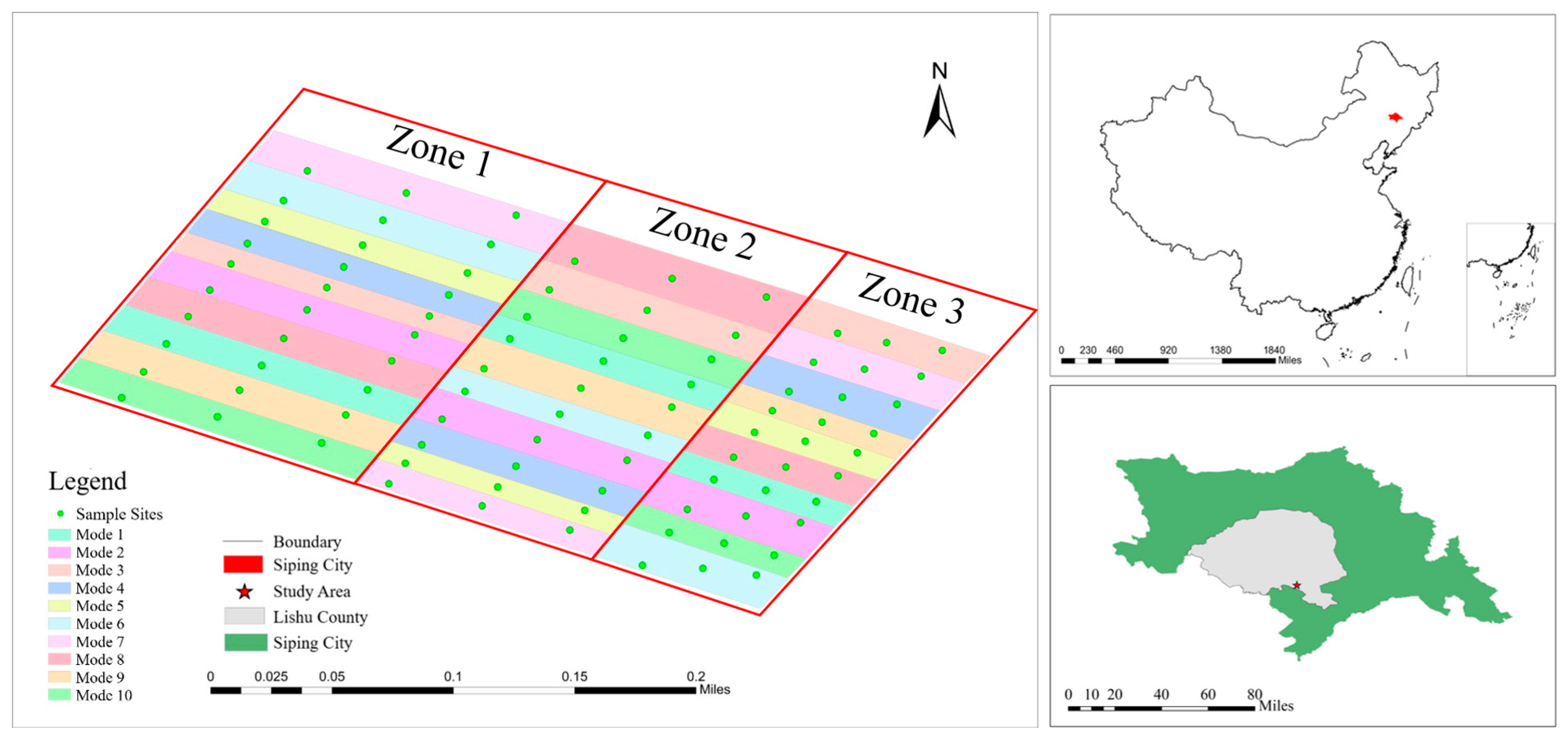
2.1. Study Area

This study was carried out in an experimental field in Lishu County (43°02′–43°46′N latitude and 123°45′–124°53′E), Jilin Province, China (Figure 1). Lishu County is a part of the Songliao Plain, located in the “three major black soil zone in the Northern Hemisphere” and “Golden Corn Belt” with fertile soil and flat terrain and has been named the “National Modern Agricultural Demonstration Zone” of China since 2011. The main soil type of the study area is black soil, which is Phaoezem according to the World Reference Base for Soil Resources [27]. The climate is a semi-humid continental monsoon type with an average annual temperature of 6.4 °C and an average annual rainfall of 493 mm, mainly concentrated in the months from April to September. The study area is located in a representative black soil zone and is an important food resource in China. Hence, choosing this region as the study area is representative and significant.

2.2. Soil Samples Collection

The experimental field consisted of three parallel zones recorded as zone 1, zone 2 and zone 3, respectively. Within each zone, ten plots were established corresponding to ten different farming practices, which are hereinafter referred to as “ten modes”, resulting in a total of thirty plots. The precise farming practices and sampling locations were distributed as illustrated in Table 1 and Figure 1.
All soil profiles were collected in June 2020, at a total depth of 1 m according to the divisions of 0–10 cm, 10–20 cm, 20–40 cm, 40–70 cm and 70–100 cm. In order of spatial location, 3 soil profiles were collected in each of the 30 plots, resulting in a total of 90 soil profiles and 450 soil samples. While collecting the soil profiles, the coordinates were measured with a real-time kinematic (RTK) AgGPS 542 global navigation satellite system (GNSS) receiver (Trimble, Ltd., Sunnyvale, CA, USA).
Table 1. The “ten modes” farming practices.
ModeTillage MethodRow SpacingStraw Returning
Mode 1Ridge Tillage60 cmNo
Mode 2Ridge Tillage60 cmYes (cover)
Mode 3Shallow Rotary Tillage40:80 cmYes (crushing)
Mode 4Deep Rotary Tillage40:80 cmYes (crushing)
Mode 5Rotary Plowing40:80 cmYes (crushing)
Mode 6No Tillage40:80 cmYes (cover)
Mode 7No Tillage40:100 cmYes (cover)
Mode 8No Tillage40:140 cmYes (cover)
Mode 9Strip Tillage40:90 cmYes (cover)
Mode 10Strip Tillage70 cmYes (cover)

2.3. Soil Spectral Measurement and Chemical Analysis

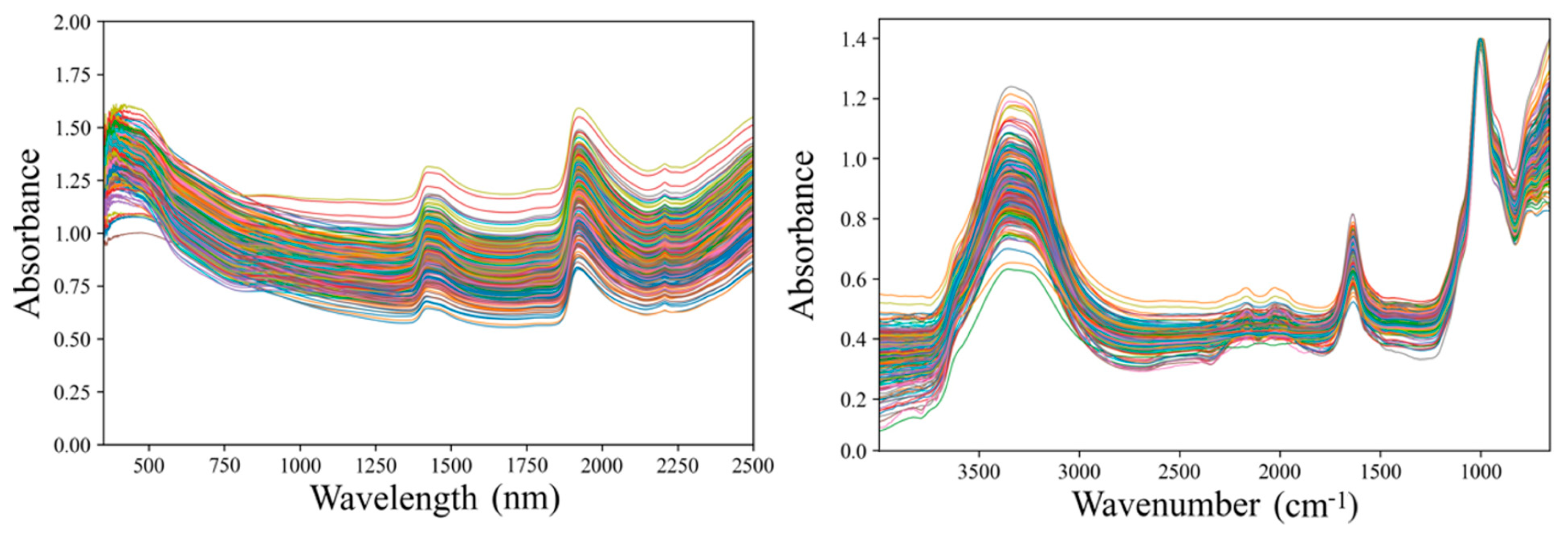
2.3.1. Soil Spectral Measurement

Each soil sample was rapidly measured for in situ spectra once it was brought to the laboratory. Subsequently, the soil sample was air-dried, ground and sieved through a 2 mm mesh. To enable laboratory chemical analysis and soil spectra measurement (referred to as “laboratory MIR” and “laboratory vis-NIR” in the following), the soil sample was partitioned into two parts.
Soil MIR spectra (both in situ and laboratory MIR) were measured using a 4300 handheld Fourier transform infrared spectrometer (Agilent Technologies, Santa Clara, CA, USA) with a spectral range of 4000–650 cm−1, a sampling interval of 0.47 cm−1 and a resolution of 4 cm−1. In this study, an attenuated total reflection (ATR) probe and a diffuse reflectance probe were used to measure in situ and laboratory spectra of soil samples, respectively. The in situ MIR was measured using an ATR probe. Soil samples (no less than 10 mm thick) were placed in plastic Petri dishes (90 mm in diameter and 15 mm in height). When placing soil samples, it is important to avoid excessive gaps, rocks or other sundries. After measuring the in situ MIR, the soil samples were air-dried, ground and sieved. Laboratory spectra were also measured in plastic Petri dishes with the soil samples no less than 10 mm thick. The laboratory MIR was measured using a diffuse reflectance probe. Both in situ spectra and laboratory spectra were determined after 3 repeated measurements for each soil sample, with 32 internal scans for each measurement, and the final records were the spectral data calculated by averaging. The instrument was calibrated every 10 min.
Soil vis-NIR spectra (both in situ and laboratory vis-NIR) were measured using a portable spectrometer (QualitySpec Trek, Analytical Spectral Devices Inc., Boulder, CO, USA) with a wavelength range of 350–2500 nm and spectral resolutions of 3 nm, 9.8 nm and 8.1 nm at 700 nm, 1400 nm and 2100 nm, respectively, with calibration provided in the form of a built-in whiteboard reference and wavelength calibration. Soil samples were also placed in plastic Petri dishes. Three replicate measurements were performed for each sample, with 50 internal scans performed for each measurement to maximize the signal-to-noise ratio of the spectra, and the average of the replicate measurements was used as the final spectral data for that soil sample. The instrument was calibrated every 10 min.

2.3.2. Chemical Analysis

Chemical analyses included the TN and TP. The TN was determined by an elemental analyzer (FLASH2000, Thermo Fisher Scientific, MA, USA). The TP was determined by a continuous flow analyzer type (AA3, Bran + Luebbe GmbH, Norderstedt, Germany).

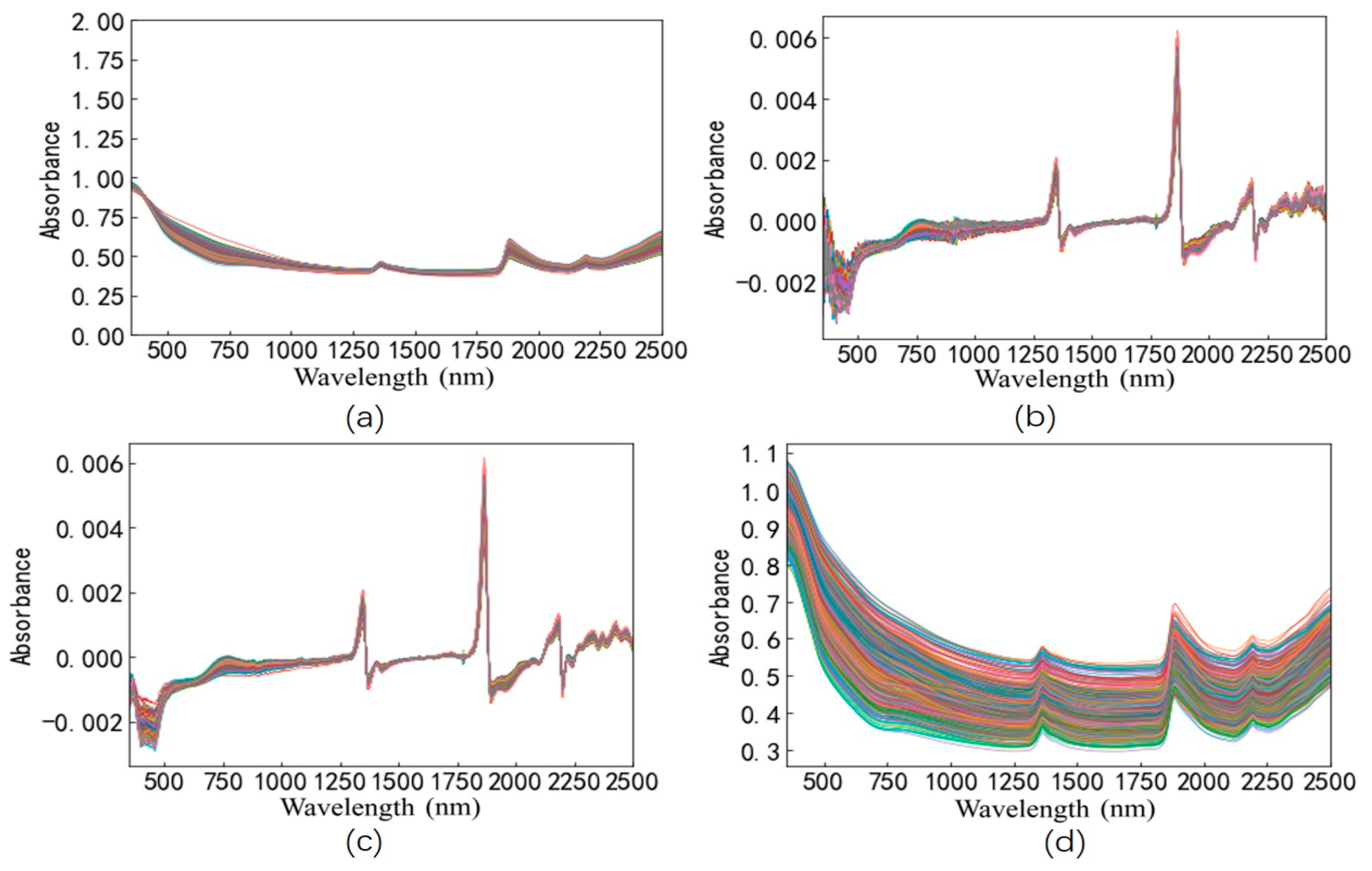
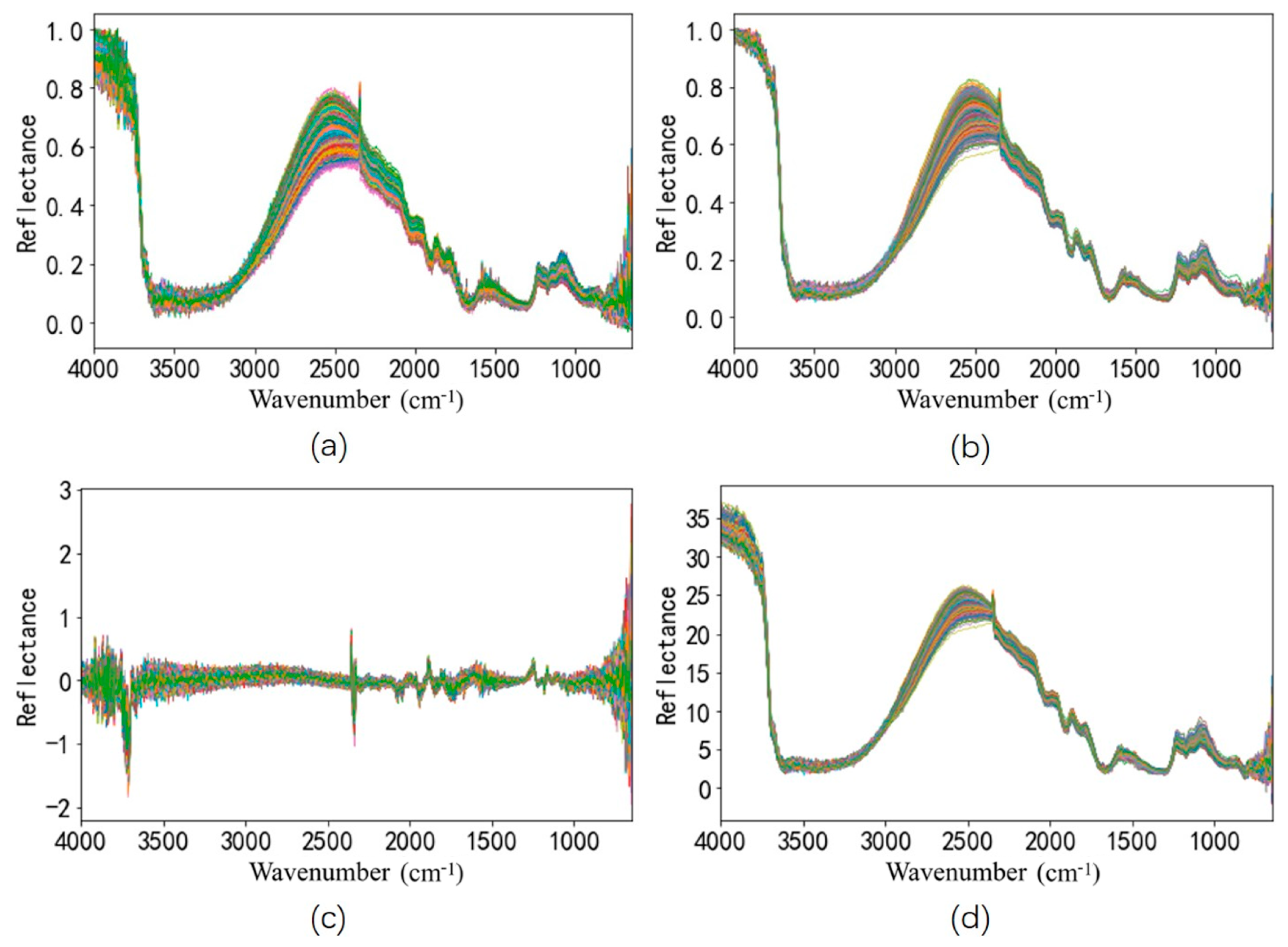
2.4. Pre-Processing of Spectra

The purpose of spectral preprocessing is to highlight the important information in the spectral data. Frequently-used methods include absorbance conversion (ABS), first derivative (FD), Savitzky–Golay convolutional smoothing (SG) and multiple scattering correction (MSC) [28,29,30]. Moreover, maximum normalization (MAN) was adopted as an alternative pre-processing method in this study.
MAN is a method of standardization aiming to scale the data so that they are distributed in a fixed interval, which facilitates data management and analysis, and allows easy comparison of data in different units. It performs a linear transformation on the original data, such that the maximum value of the data is normalized to 1, while the other data are proportionally scaled to the range of 0 to 1.
In this study, laboratory MIR and vis-NIR were used to compare the effects of different spectral pre-processing combinations and to select the optimal spectral pre-processing combination for MIR and vis-NIR. Multivariate adaptive regression splines (MARS) was chosen as the modeling method.

2.5. Soil Spectral Predictive Algorithms

2.5.1. Partial Least Squares Regression

Partial least squares regression (PLSR) was proposed by Wold et al. in 1983 [31], integrating the ideas of multiple regression, principal component analysis and correlation analysis, and having a great advantage in dealing with problems in which the number of independent variables is much larger than the number of samples. It can effectively eliminate the problem of multicollinearity among the variables and is currently one of the most commonly used algorithms in the field of soil hyper-spectroscopy. Based on it, various prediction models for the prediction of soil properties have been successfully established.
In addition, in order to find the feature bands and to elucidate the different prediction performances of different models and spectra, this study used the PLS-VIP method to calculate the scores of variable importance in the projection (VIP) [32,33]. The v j weights are measures of the contribution of each variable according to the variance explained by each PLS component where ( w a j / | w a | ) 2 represents the importance of the jth variable. Since the variance explained by each component can be computed by the expression q a 2 t a t a , the v j can be expressed as [34,35]:
v j = p a = 1 A [ ( q a 2 t a t a ) ( w a j / | w a | ) 2 ] / a = 1 A ( q a 2 t a t a )  
Variable j can be eliminated if v j < u for some user-defined threshold u [ 0 , ) . It is generally accepted that a variable should be selected if v j > 1.
The PLSR in the study was carried out from the “sklearn” package in Python 3.8.8. The main parameter of the PLSR model is the number of components to keep (n_components). The PLS-VIP method in the study was carried out from the plsVarSel package [36] with R 4.2.2 [37].

2.5.2. Multivariate Adaptive Regression Splines

Multivariate adaptive regression splines (MARS) is a segmented linear regression model for high-dimensional data proposed by American statistician Friedman in 1991 [38]. MARS divides a whole region into several small intervals and creates a polynomial within each interval, which maintains both the continuity of the model as a whole and the independence of the intervals from each other. MARS has the following features: (1) the nodes and basic functions are automatically determined through the forward and backward pruning process, which has an extremely strong self-adaptability and the advantages of fast computation and an accurate model in processing high-dimensional data; (2) each segment polynomial has a certain degree of smoothness at the interval connection, which maintains both the continuity of the model as a whole and the local independence between the intervals and can effectively extract the linear and nonlinear relationships between variables; (3) it has good interpretability.
The MARS in the study was carried out from the “pyearth” package in Python 3.8.8. The main parameters of the MARS model include the maximum degree of terms generated by the forward pass (max_degree), the maximum number of terms generated by the forward pass (max_terms) and whether the model will be smoothed such that it has continuous first derivatives (smooth).

2.5.3. Random Forest

Random forest (RF) is an integrated learning algorithm proposed by Breiman in 2001 [39], which uses the Bagging integration idea based on a CART decision tree and introduces random attributes in the training process of the decision tree. With a simple algorithm, good generalization effect and easy implementation, it is now widely used in the field of soil hyperspectral modeling. The main idea of the Bagging algorithm is that given a data set of size m samples, a sample is randomly taken out with put-back and added to the training set, and repeated m times. A training set containing m samples can be obtained with great probability that some samples are not selected and some samples are selected several times [40]. The basic idea of RF is that for a data set of m samples, the Bagging algorithm is used to randomly obtain m training sets and repeat n times to get n different training sets and establish n CART decision trees, with important parameters such as the number of trees, the maximum depth of the trees, the maximum number of feature choices, etc. The result is the vote (classification problem) or the average (regression problem) of the n decision trees.
The RF in the study was carried out from the “sklearn” package in Python 3.8.8. The main parameters of the RF model include the number of trees (n_estimators), the minimum sample number of selected factors in each node (min_samples_leaf), the maximum depth of trees (max_depth) and the maximum features considered (max_features).

2.5.4. Data Splitting

In this study, 90 soil profiles with a total of 450 soil samples were divided into training and validation sets according to parallel zones. Soil samples from zones 1 and 2 were used as the training set (n = 300) and soil samples from zone 3 were used as the validation set (n = 150).

2.6. Model Assessment

In this study, the coefficient of determination (R2), the root mean square error (RMSE) and the ratio of standard deviation to RMSE (RPD) were used as the evaluation indexes of the model prediction performance. Chang et al. (2001) classified models into three classes based on the RPD values: when the RPD < 1.4, it is an unreliable model, and the model does not have predictive ability; when 1.4 < RPD < 2, it is a reliable model, and the model has good predictive ability; when the RPD > 2, it is an excellent model, and the model has excellent predictive ability [41]. In general, an optimal model has a higher R2 and RPD, and a lower RMSE. The calculation formulas are as follows:
R 2 = 1 i = 1 n ( y o b s y p r e d ) 2 i = 1 n ( y o b s y ¯ ) 2  
RMSE = 1 / n i = 1 n ( y o b s y p r e d ) 2  
RPD = SD / RMSE = [ 1 / ( n 1 ) i = 1 n ( y p r e d y ¯ ) 1 / n i = 1 n ( y o b s y p r e d ) ] 1 / 2  
where y o b s and y p r e d are the true and predicted values, respectively; y ¯ is the mean of y o b s ; n is the number of samples.

3. Results

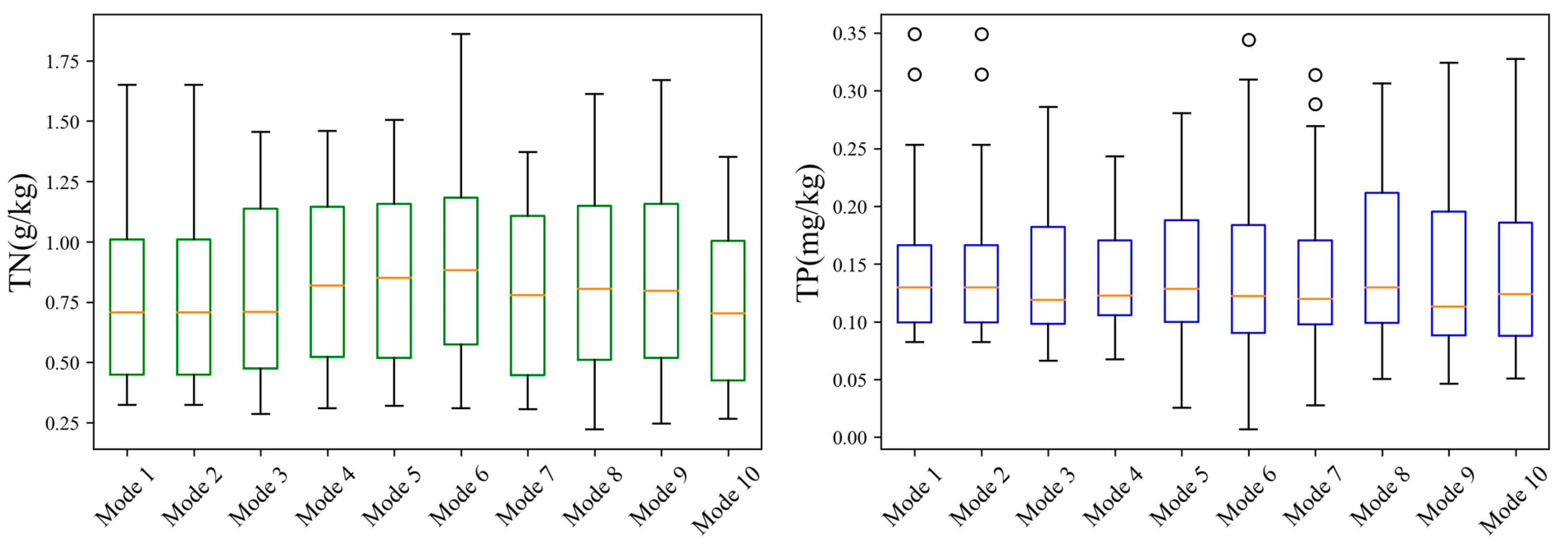
3.1. Soil Properties Distribution

Statistical information on the properties of all 450 soil samples is shown in Table 2. Moreover, the whole dataset, training set and validation set all had normally distributed TP and TN data. Different farming practices have different effects on soil properties; scientific management methods (such as straw returning and no tillage) can not only improve soil fertility but also increase field water use efficiency [42,43,44]. Figure 2 shows the situation of soil properties (including TN and TP) under different farming practices. Mode 6 is higher than other farming practices in terms of lower quartile and median for the TN. This might be because no tillage and straw returning can minimize tillage and leave crop residues on the soil surface for natural decomposition, which results in reduced soil disturbance, improved soil surface coverage, suppressed mineralization and input of soil organic matter and ultimately increased soil organic matter content [45].
Table 2. Statistical description table of soil sample properties.
Soil
Properties
Whole Dataset (450)Training Set (300)Validation Set (150)
Min.MeanMax.SDMin.MeanMax.SDMin.MeanMax.SD
TN (g/kg)0.220.821.860.370.220.841.860.360.280.791.650.35
TP (mg/kg)7.00145.26591.9671.137.00156.03591.9670.2525.70124.28323.7965.49

3.2. Comparison of Spectra Pre-Processing Combinations

From vis-NIR after different spectral preprocessing combinations (Figure 3), it can be seen that the spectral data generated by the combinations were more concentrated except ABS+SG. The spectral differences were more obvious after the first derivatives, but there was also more noise. From MIR after different spectral preprocessing combinations (Figure 4), it can be seen that the spectral data without SG smoothing but using the first derivative had obvious noise, while the MIR processed by MSC+SG were more concentrated compared with that of SG+MAN.
All pre-processing combinations can successfully predict the soil TN (R2 = 0.79–0.81, RMSE = 0.15–0.16 g/kg, RPD = 2.12–2.31), but the soil TP was poorly predicted in all combinations (R2 = 0.25–0.48, RMSE = 46.93–56.71 mg/kg, RPD = 1.16–1.40). For vis-NIR, ABS+SG achieved the highest accuracy (for TN: R2 = 0.81, RMSE = 0.15 g/kg, RPD = 2.31; for TP: R2 = 0.48, RMSE = 46.93 mg/kg, RPD = 1.40); for MIR, SG+MAN achieved the highest accuracy (for TN: R2 = 0.90, RMSE = 0.11 g/kg, RPD = 3.11; for TP: R2 = 0.33, RMSE = 52.60 mg/kg, RPD = 1.23) (Table 3). As a result, the ABS+SG combination (polynomial of 2 and window width of 15) combination was used in this study for vis-NIR, and the SG+MAN combination (polynomial of 2 and window width of 11) combination was used for MIR. The values of “polynomial” and “window width” were finally selected according to prediction accuracy after being widely tested. Figure 5 shows the in situ vis-NIR and MIR with the best pre-processing combination methods.
Table 3. Prediction accuracy of soil properties based on vis-NIR and MIR with different spectral pre-processing combinations.
Soil PropertiesSpectral Preprocessing CombinationsR2RMSERPD
vis-NIR
TN (g/kg)ABS+FD0.790.162.23
ABS+SG0.810.152.31
ABS+SG+FD0.780.162.12
ABS+MSC+SG0.800.162.24
TP (mg/kg)ABS+FD0.2656.091.17
ABS+SG0.4846.931.40
ABS+SG+FD0.3950.891.29
ABS+MSC+SG0.2556.711.16
MIR
TN (g/kg)MSC+MAN0.880.113.00
SG+MAN0.900.113.11
SG+FD0.790.162.21
MSC+SG0.810.152.31
TP (mg/kg)MSC+MAN0.2157.261.13
SG+MAN0.3352.601.23
SG+FD0.2555.691.16
MSC+SG0.2157.211.11
ABS: absorbance conversion; FD: first derivative; SG: Savitzky-Golay convolutional smoothing; MSC: multiple scattering correction; MAN: maximum normalization

3.3. Prediction of Soil Properties Based on in situ Spectra

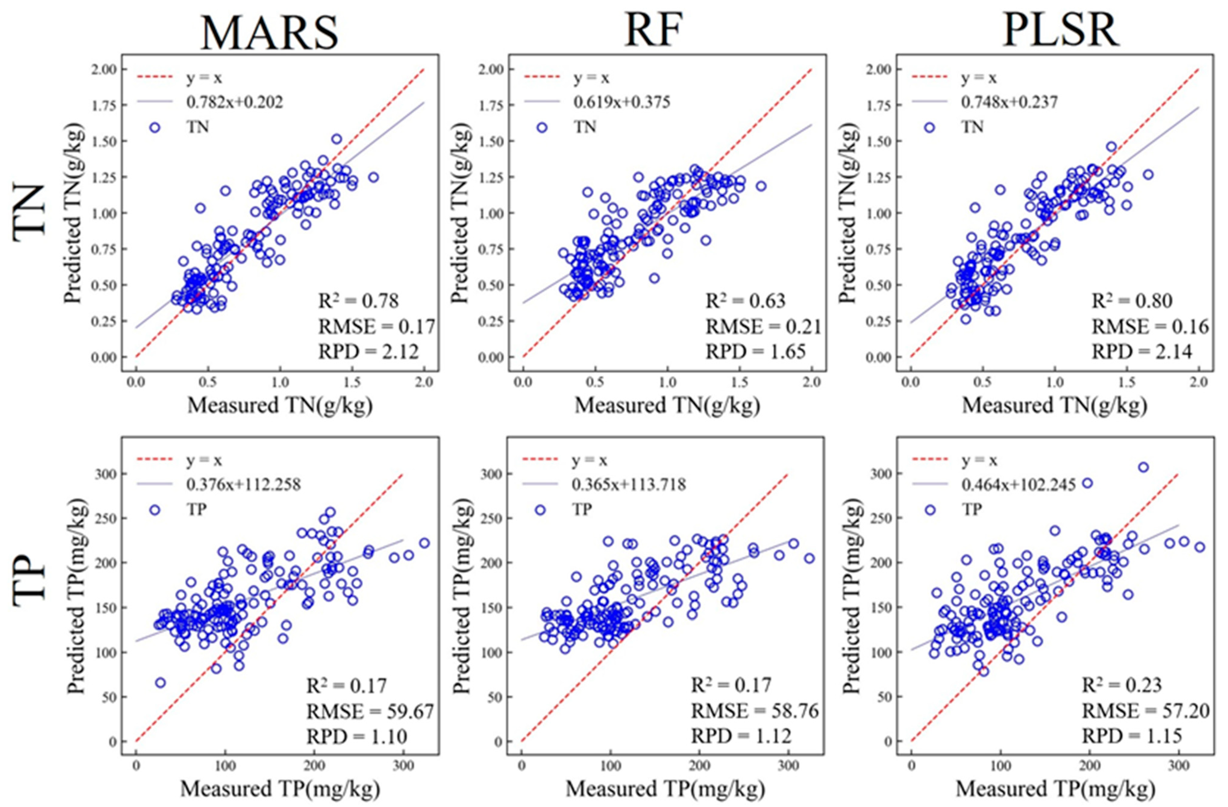
3.3.1. Prediction of Soil Properties Based on in situ vis-NIR

All models based on in situ vis-NIR could successfully predict the TN (R2 = 0.63–0.80, RMSE = 0.16–0.21 g/kg, RPD = 1.65–2.14), but could not predict the TP (R2 = 0.17–0.23, RMSE = 57.20–59.67 mg/kg, RPD = 1.10–1.15). For the TN, the performances of MARS and PLSR models based on in situ vis-NIR were similar, and the prediction accuracy of the RF model was relatively lower. The MARS model had an R2 of 0.78, a RMSE of 0.17 g/kg with a RPD of 2.12; the PLSR model had an R2 of 0.80, a RMSE of 0.16 g/kg with a RPD of 2.14; the RF model had an R2 of 0.63, a RMSE of 0.21 g/kg with a RPD of 1.65. For the TP, the performances of the MARS and RF models based on in situ vis-NIR were similar, and the prediction accuracy of the PLSR model was relatively higher. The MARS model had an R2 of 0.17, a RMSE of 59.67 mg/kg with a RPD of 1.10; the RF model had an R2 of 0.17, a RMSE of 58.76 mg/kg with a RPD of 1.12; the PLSR model had an R2 of 0.23, a RMSE of 57.20 mg/kg with a RPD of 1.15 (Figure 6 and Table 4).

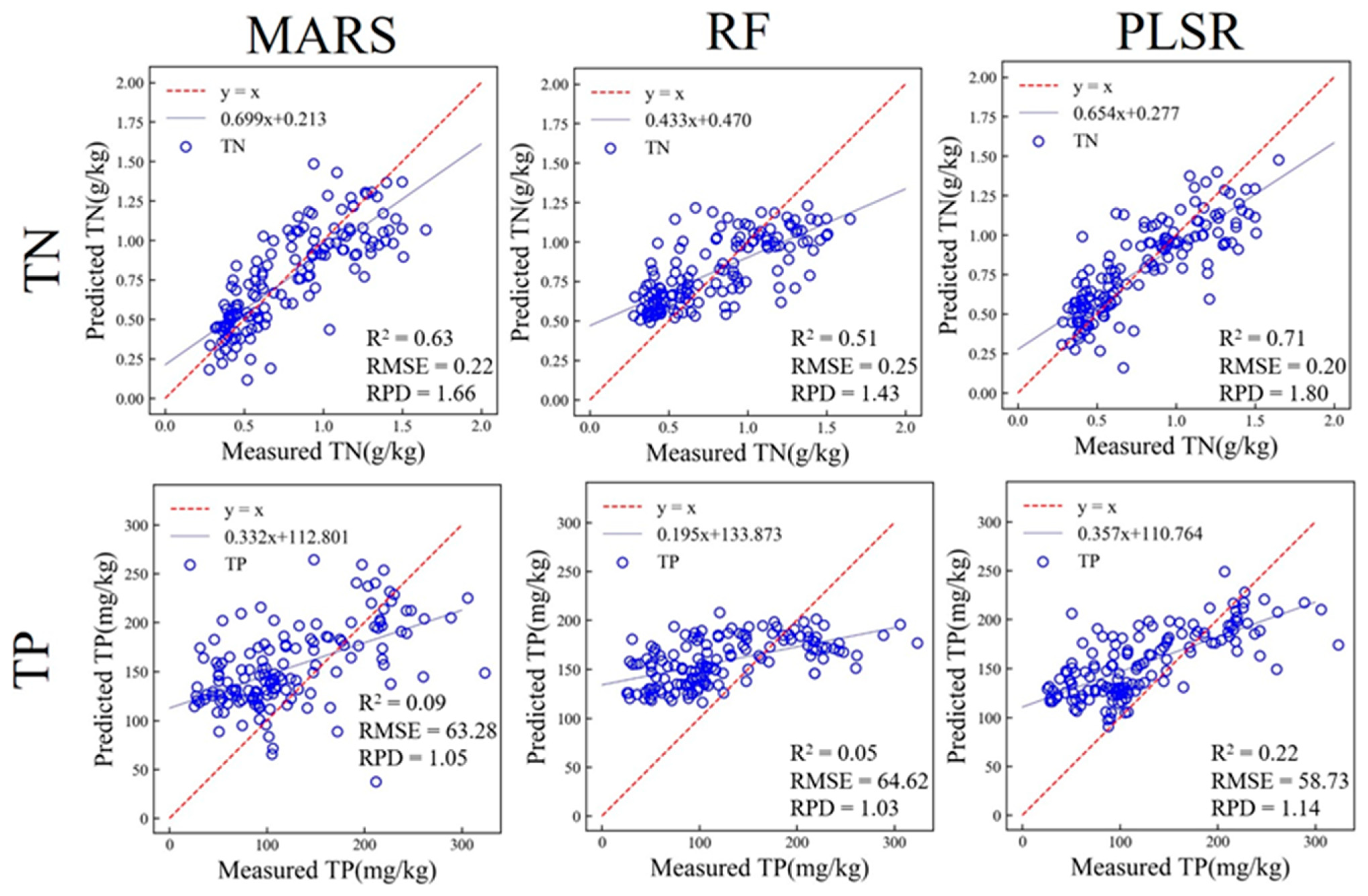
3.3.2. Prediction of Soil Properties Based on in situ MIR

Similarly, all models based on in situ MIR could successfully predict the TN (R2 = 0.51–0.71, RMSE = 0.20–0.25 g/kg, RPD = 1.43–1.80), but could not predict the TP (R2 = 0.05–0.22, RMSE = 58.73–64.62 mg/kg, RPD = 1.03–1.14). Meanwhile, it can be seen that the prediction accuracy of in situ MIR was relatively lower than that of in situ vis-NIR. For the TN, the prediction accuracy of the PLSR model based on in situ MIR was the highest, while the prediction accuracy of the RF model was the lowest. The PLSR model had an R2 of 0.71, a RMSE of 0.20 g/kg with a RPD of 1.80; the MARS model had an R2 of 0.63, a RMSE of 0.22 g/kg with a RPD of 1.66; the RF model had an R2 of 0.51, a RMSE of 0.25 g/kg with a RPD of 1.43. For the TP, the performances of the MARS and RF models based on in situ MIR were similar, and the prediction accuracy of the PLSR model was relatively higher. The MARS model had an R2 of 0.09, a RMSE of 63.28 mg/kg with a RPD of 1.05; the RF model had an R2 of 0.05, a RMSE of 64.62 mg/kg with a RPD of 1.03; the PLSR model had an R2 of 0.22, a RMSE of 58.73 mg/kg with a RPD of 1.14 (Figure 7 and Table 4).
Both in situ vis-NIR and MIR could successfully predict the TN, but could not predict the TP. The prediction accuracy of in situ MIR was relatively lower than that of in situ vis-NIR. The optimal model was the PLSR.

3.4. Prediction of Soil Properties Based on Laboratory Spectra

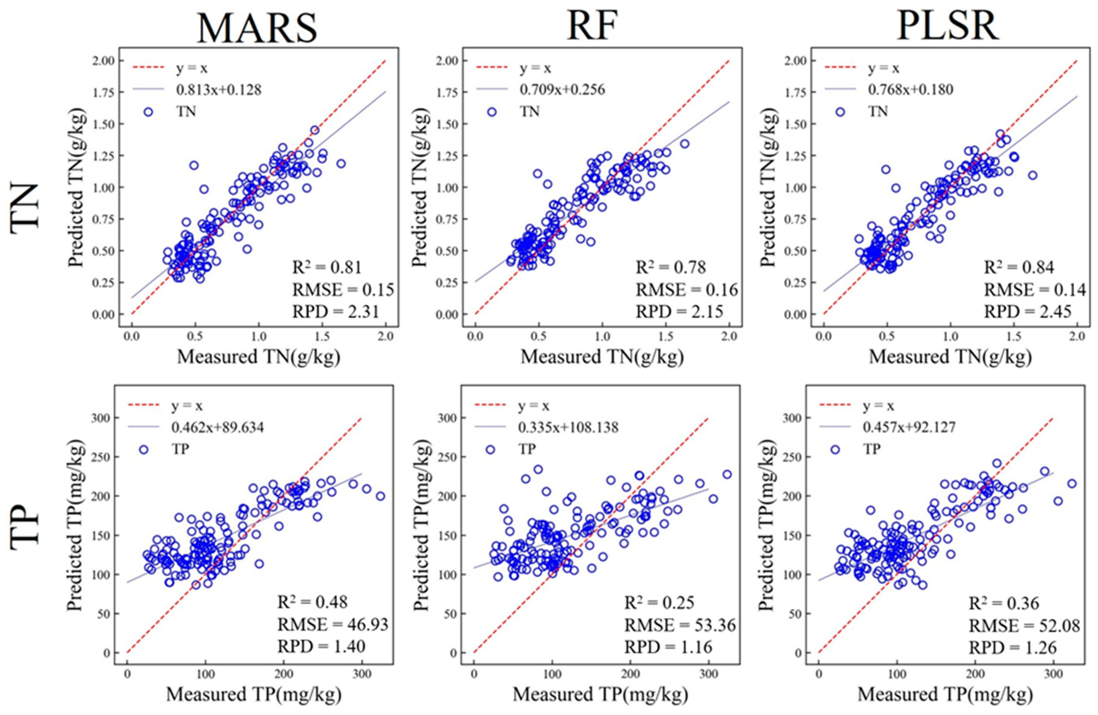
3.4.1. Prediction of Soil Properties Based on Laboratory vis-NIR

All models based on laboratory vis-NIR could successfully predict the TN (R2 = 0.78–0.84, RMSE = 0.14–0.16 g/kg, RPD = 2.15–2.45), but could not predict the TP (R2 = 0.25–0.48, RMSE = 46.93–53.36 mg/kg, RPD = 1.16–1.40). Meanwhile, it can be seen that the prediction accuracy of laboratory vis-NIR was higher than that of in situ vis-NIR and MIR. For the TN, the prediction accuracy of the PLSR model based on laboratory vis-NIR was the highest, while the prediction accuracy of the RF model was the lowest. The PLSR model had an R2 of 0.84, a RMSE of 0.14 g/kg with a RPD of 2.45; the MARS model had an R2 of 0.81, a RMSE of 0.15 g/kg with a RPD of 2.31; the RF model had an R2 of 0.78, a RMSE of 0.16 g/kg with a RPD of 2.15. For the TP, the prediction accuracy of the MARS model based on laboratory vis-NIR was the highest, while the prediction accuracy of the RF model was the lowest. The MARS model had an R2 of 0.48, a RMSE of 46.93 mg/kg with a RPD of 1.40, but its accuracy on the training set was too low to be identified as a reliable model; the PLSR model had an R2 of 0.36, a RMSE of 52.08 mg/kg with a RPD of 1.26; the RF model had an R2 of 0.25, a RMSE of 53.36 mg/kg with a RPD of 1.16 (Figure A1 and Table 4).

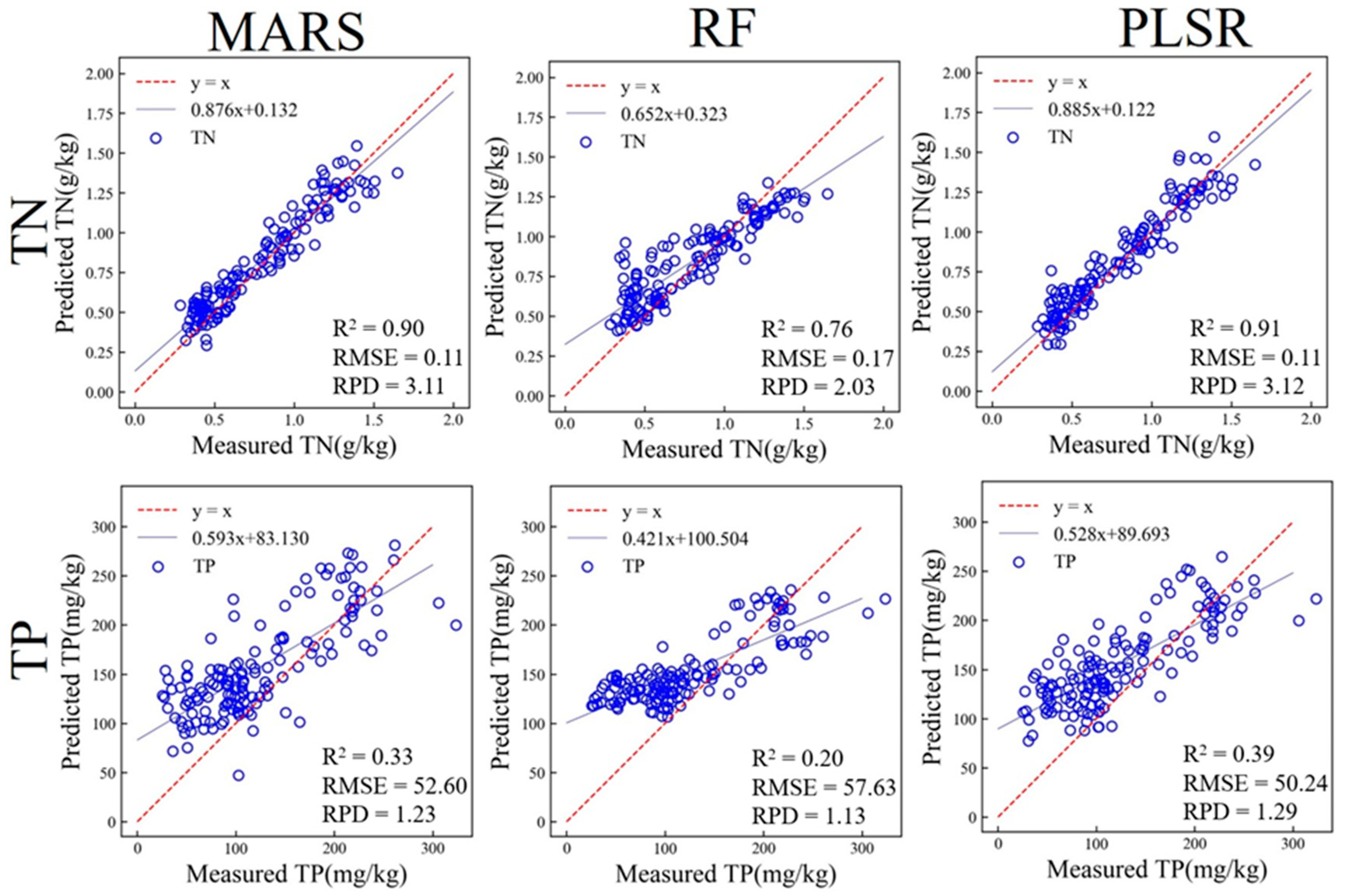
3.4.2. Prediction of Soil Properties Based on Laboratory MIR

Similarly, all models based on laboratory MIR could successfully predict the TN (R2 = 0.76–0.91, RMSE = 0.11–0.17 g/kg, RPD = 2.03–3.12), but could not predict the TP (R2 = 0.20–0.39, RMSE = 50.24–57.63 mg/kg, RPD = 1.13–1.29). Meanwhile, it can be seen that the prediction accuracy of laboratory MIR was the highest among the four kinds of spectra. For the TN, the prediction accuracy of the PLSR model based on laboratory MIR was the highest, while the prediction accuracy of the RF model was the lowest. The PLSR model had an R2 of 0.91, a RMSE of 0.11 g/kg with a RPD of 3.12; the MARS model had an R2 of 0.90, a RMSE of 0.11 g/kg with a RPD of 3.11; the RF model had an R2 of 0.76, a RMSE of 0.17 g/kg with a RPD of 2.03. For the TP, the performances of the MARS and PLSR models based on in situ MIR were similar, and the prediction accuracy of the RF model was relatively lower. The PLSR model had an R2 of 0.39, a RMSE of 50.24 mg/kg with a RPD of 1.29; the MARS model had an R2 of 0.33, a RMSE of 52.60 mg/kg with a RPD of 1.23; the RF model had an R2 of 0.20, a RMSE of 57.63 mg/kg with a RPD of 1.13 (Figure A2 and Table 4).
Both vis-NIR and MIR could successfully predict the TN, but could not predict the TP, whether in in situ or laboratory conditions. The optimal model was the PLSR. The prediction accuracy followed laboratory MIR > laboratory vis-NIR > in situ vis-NIR > in situ MIR.
Table 4. Prediction accuracy of soil TN and TP.
Soil
Properties
Modeling
Algorithms
Training SetValidation Set
R2RMSER2RMSERPD
in situ vis-NIR
TN (g/kg)MARS0.790.170.780.172.12
RF0.770.170.630.211.65
PLSR0.770.170.800.162.14
TP (mg/kg)MARS0.2461.050.1759.671.10
RF0.3656.010.1758.761.12
PLSR0.3357.340.2357.201.15
in situ MIR
TN (g/kg)MARS0.760.180.630.221.66
RF0.680.210.510.251.43
PLSR0.730.190.710.201.80
TP (mg/kg)MARS0.1366.290.0963.281.05
RF0.2561.630.0564.621.03
PLSR0.2262.850.2258.731.14
Laboratory vis-NIR
TN (g/kg)MARS0.780.170.810.152.31
RF0.870.130.780.162.15
PLSR0.750.180.840.142.45
TP (mg/kg)MARS0.2660.370.4846.931.40
RF0.6342.270.2553.361.16
PLSR0.3755.780.3652.081.26
Laboratory MIR
TN (g/kg)MARS0.870.130.900.113.11
RF0.950.080.760.172.03
PLSR0.880.120.910.113.12
TP (mg/kg)MARS0.4552.670.3352.601.23
RF0.8329.490.2057.631.13
PLSR0.3159.010.3950.241.29
MARS: multivariate adaptive regression splines; PLSR: partial least squares regression; RF: random forest.

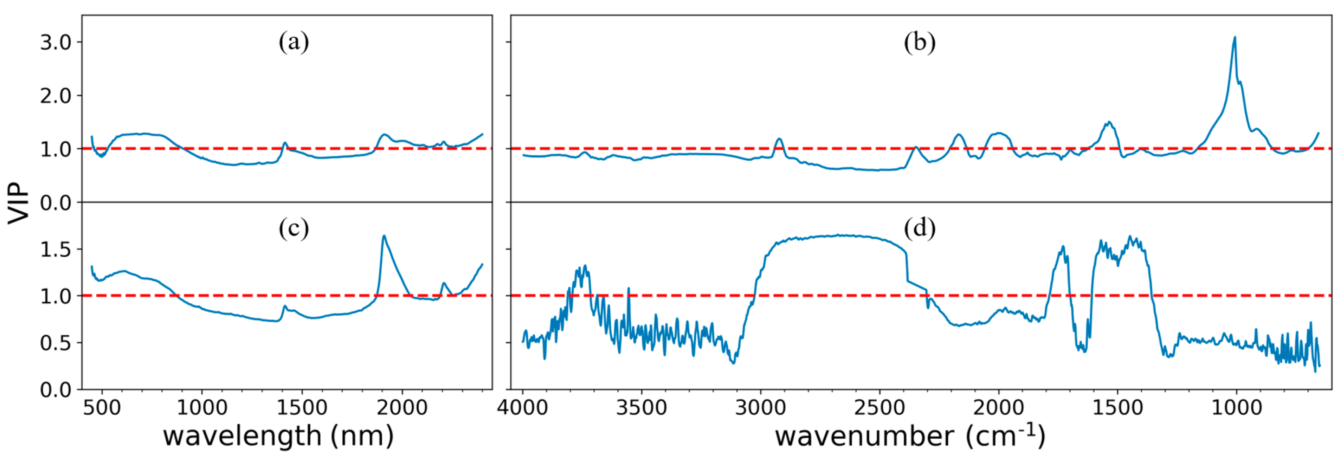
3.5. The Scores of Variable Importance in Projection (VIP)

Figure 8 shows the VIP scores of each wavelength derived from PLSR. (1) For in situ vis-NIR, feature bands included 450 nm–461 nm, 530–906 nm, 1403 nm–1433 nm and 1867 nm–2400 nm, which were 48.89% of the total (Figure 8a); (2) for in situ MIR, feature bands included 2937 cm−1–2907 cm−1, 2348 cm−1–2341 cm−1, 2199 cm−1–2139 cm−1, 2057 cm−1–1946 cm−1, 1618 cm−1–1498 cm−1, 1163 cm−1–850 cm−1 and 693–656 cm−1, which were 21.83 % of the total (Figure 8b); (3) for laboratory vis-NIR, feature bands included 450 nm–872 nm, 1874 nm–2041 nm and 2190 nm–2400 nm, which were 41.11% of the total (Figure 8c); (4) for laboratory MIR, feature bands included 3809 cm−1–3802 cm−1, 3791 cm−1–3716 cm−1, 3686 cm−1, 3660 cm−1, 3556 cm−1–3554 cm−1, 3025 cm−1–2303 cm−1, 1785 cm−1–1702 cm−1 and 1606 cm−1–1359 cm−1, which were 32.84% of the total (Figure 8d). For in situ spectra, in situ vis-NIR had the highest proportion of feature bands, but with the lowest average VIP scores, while in situ MIR had the lowest proportion of feature bands along with low average VIP scores except for an extreme high peak of VIP scores around 1006 cm−1. For laboratory spectra, laboratory vis-NIR had a similar waveshape of VIP scores with in situ vis-NIR, and with higher peaks, while laboratory MIR had an unsimilar waveshape of VIP scores with in situ vis-NIR and had the steadiest feature bands and relatively higher values. As a whole, there were more feature bands along with higher VIP scores in laboratory spectra.

4. Discussion

4.1. Prediction Performance of Soil Properties Using in situ vs. Laboratory Spectra

This study indicated that the prediction performance of spectra followed laboratory MIR > laboratory vis-NIR > in situ vis-NIR > in situ MIR, and which of the models followed PLSR > MARS > RF. In general, complex machine learning algorithms (e.g., RF) generally appear to provide better model performance than linear models (e.g., PLSR) at a regional scale, whereas the most appropriate model might be case specific [46]. In the field scale, linear regression may be suitable for predicting some soil properties (e.g., EC, salinity), which might be attributed to low spatial variability [47,48]. The prediction accuracy of laboratory MIR was higher than that of laboratory vis-NIR, which is consistent with the findings of previous studies [49,50,51,52,53,54,55]. This is mainly due to the presence of a large number of correlated feature peaks within the MIR band, and the fact that the fundamental frequency vibration between the molecules of the substance occurs in the MIR band, while the vis-NIR band range exists as multiplication and co-frequency vibrations of the fundamental frequency vibrations in the MIR band [56]. The prediction accuracy of in situ MIR was lower than that of in situ vis-NIR, which is consistent with the findings of previous studies [25,53]. This is mainly due to the presence of octave and ensemble peaks in the vis-NIR band range, while the MIR band range is dominated by the fundamental frequency peaks of soil property groups and moisture effects are mainly due to the 3600 cm−1–2800 cm−1 range of the O–H bond stretching vibrations, so the MIR are more influenced by soil moisture compared to vis-NIR [57,58,59]. In addition, the TP cannot be predicted quantitatively mainly because there was no direct feature band on both spectra regarding the TP, while the correlation between the TP and TN was not significant. Similar results were reported by some previous studies [60,61,62].

4.2. The Feature Bands of TN Prediction with the Four Kinds of Spectra

This study used the PLS-VIP method to find the feature bands of MIR and vis-NIR spectra in in situ and laboratory conditions for TN prediction. in situ vis-NIR kept a similar waveshape of VIP scores with laboratory vis-NIR while in situ MIR did not, indicating that the disturbance of in situ conditions made a bigger influence on MIR, especially in the feature bands of soil moisture, which covered the feature bands of TN. The extreme high peak of VIP scores in 1006 cm−1 might come from the quartz [63]. Laboratory spectra had more feature bands along with higher VIP scores, and laboratory MIR had the steadiest feature bands and relatively higher values, which may indicate the reason why the best prediction performance came from laboratory MIR. Much information is hidden in the differences between in situ MIR and laboratory MIR, and further studies need to be carried out in the future. To our knowledge, there were no such studies in the past. However, there were some related studies that could be mutual corroborations with this study. Greenberg et al. [51] found that optimal MIR models always used 4000 cm−1–3682.1 cm−1 and 3020.5 cm−1–1693.5 cm−1 bands in predicting TN since the bands below 1000 cm−1 were believed to contain more noise and overlapping peaks of organic and mineral compounds [10,64]. The optimal vis-NIR models always used 834 nm–1167 nm and 2166 nm–2500 nm bands. In addition, the important peaks with large loadings values for TN prediction models were at 536 nm, 570 nm, 652 nm, 686 nm, 1402 nm, 1420 nm, 1898 nm, 2200 nm, 2300 nm and 2430 nm in vis-NIR, and at 3700 cm−1, 3591 cm−1, 2960 cm−1, 2208 cm−1, 2035 cm−1, 1907 cm−1, 1853 cm−1, 1400 cm−1 and 1280 cm−1 in MIR. Xu et al. [65] used the stepwise regression method to analyze the relationships between the absorption features of laboratory vis-NIR and nitrogen concentration to select the absorption features significantly correlated with nitrogen, and found some strong absorption bands centered on 410 nm, 480 nm, 1910 nm and 2470 nm. Lu et al. [66] finished a study on searching the feature bands of TN, including 429 nm, 492 nm, 556 nm, 628 nm, 978 nm, 1066 nm, 1181 nm, 1202 nm, 1240 nm, 1274 nm, 1305 nm, 1329 nm, 1486 nm, 1514 nm, 1523 nm, 1566 nm, 1599 nm, 1642 nm, 1760 nm and 2491 nm.

4.3. Feasibility Analysis for Rapid Prediction of Soil Properties Based on in situ MIR

Although in situ MIR had lower prediction accuracy compared to laboratory spectra, it is still a feasible and practical method for predicting soil properties [67]. In contrast to laboratory spectral acquisition, in situ MIR is time-saving and cost-effective [68,69]. This feature is particularly helpful for promoting large-area soil surveys and mapping, where relative information on soil properties and their spatial variability may be more important than the accuracy of a few single-point values [70]. In terms of the predicted soil TN and TP, in situ MIR can successfully predict the TN. The optimal RPD value was 1.80 and the RMSE was 0.20 g/kg, which was a reliable prediction model. The highest RPD for the TP was only 1.14 and the RMSE was 58.73 mg/kg, which could not be predicted successfully. In terms of modeling methods, both the MARS and PLSR models can successfully build prediction models for soil properties based on in situ MIR, among which PLSR had the best overall performance, with R 2 reaching 0.71 for the prediction of TN. In terms of comparison with laboratory spectra, the accuracy of the in situ MIR spectral model was lower than that of the laboratory vis-NIR and MIR models, mainly because in situ MIR was more influenced by soil moisture [47,70], which covered the spectral features of soil properties in MIR. In terms of experimental convenience, the acquisition of laboratory spectra required soil sample collection, bagging and transportation, air-drying, grinding and sieving operations, which consumed a lot of time, and labor costs and were not conducive to the promotion of large-area soil property investigation applications, while in situ spectral acquisition can save a lot of operations by simply applying a portable spectrometer directly to acquire in situ spectra, which is of great significance to the promotion of soil remote sensing to larger areas.

5. Conclusions

This study verified the ability of in situ MIR for soil property prediction and confirmed the potential of extending the advantages of MIR from laboratory to in situ. Moreover, the modeling performances using MIR and vis-NIR spectra collected in in situ and laboratory conditions were compared.
The detailed results are as follows: (i) the best spectral pre-processing combination for MIR is SG+MAN, and the best spectral pre-processing combination for vis-NIR is ABS+SG; (ii) in situ MIR can successfully predict the TN with a RPD of 1.80 and RMSE of 0.20 g/kg (neither MIR nor vis-NIR could predict the TP quantitatively), which greatly simplifies the experimental content and demonstrates its application value in the field of large-area soil investigation and mapping; (iii) the prediction performance followed laboratory MIR > laboratory vis-NIR > in situ vis-NIR > in situ MIR.
This study provided an approach for rapid soil information obtaining and a reference for soil research and management in black soil areas. More efforts should be made in the future, especially on appropriate measuring methods and analyzing algorithms for in situ MIR.

Author Contributions

Conceptualization, W.J.; methodology, J.Y. and Z.S. (Zhan Shi); software, Z.S. (Zhan Shi) and J.Y.; validation, Z.S. (Zhan Shi) and J.Y.; formal analysis, J.Y. and Z.S. (Zhan Shi).; investigation, Z.S. (Zhan Shi) and T.M.; resources, W.J.; data curation, Z.S. (Zhan Shi) and J.Y.; writing—original draft preparation, J.Y. and Z.S. (Zhan Shi); writing—review and editing, W.J., B.L, F.S., Z.S. (Zhou Shi), S.C. and M.Y.; visualization, J.Y. and Z.S. (Zhan Shi); supervision, W.J. and B.L.; project administration, W.J.; funding acquisition, W.J. All authors have read and agreed to the published version of the manuscript.

Funding

The study was supported by the National Natural Science Foundation of China (42001048), the National Key R&D Program of China (2021YFD1500201), the Open Fund of State Key Laboratory of Remote Sensing Science (OFSLRSS202121), and the State Key Laboratory of Resources and Environmental Information System (2020).

Data Availability Statement

The data presented in this study are available upon request from the corresponding author.

Conflicts of Interest

The authors declare no conflict of interest.

Appendix A

Figure A1. Scatter plot of soil TN and TP prediction based on laboratory vis-NIR.
Remotesensing 15 02053 g0a1
Figure A2. Scatter plot of predicted soil TN and TP based on laboratory MIR.
Remotesensing 15 02053 g0a2

References

  1. Yang, X.M.; Zhang, X.P.; Deng, W.; Fang, H.J. Black Soil Degradation by Rainfall Erosion in Jilin, China. Land Degrad. Dev. 2003, 14, 409–420. [Google Scholar] [CrossRef]
  2. Zheng, H.; Liu, W.; Zheng, J.; Luo, Y.; Li, R.; Wang, H.; Qi, H. Effect of Long-Term Tillage on Soil Aggregates and Aggregate-Associated Carbon in Black Soil of Northeast China. PLoS ONE 2018, 13, e0199523. [Google Scholar] [CrossRef]
  3. Xu, X.Z.; Xu, Y.; Chen, S.C.; Xu, S.G.; Zhang, H.W. Soil Loss and Conservation in the Black Soil Region of Northeast China: A Retrospective Study. Environ. Sci. Policy 2010, 13, 793–800. [Google Scholar] [CrossRef]
  4. Zhang, M.; Hou, R.; Li, T.; Fu, Q.; Zhang, S.; Su, A.; Xue, P.; Yang, X. Study of Soil Nitrogen Cycling Processes Based on the 15N Isotope Tracking Technique in the Black Soil Areas. J. Clean. Prod. 2022, 375, 134173. [Google Scholar] [CrossRef]
  5. Rossel, R.V.; Walvoort, D.J.J.; McBratney, A.B.; Janik, L.J.; Skjemstad, J.O. Visible, near Infrared, Mid Infrared or Combined Diffuse Reflectance Spectroscopy for Simultaneous Assessment of Various Soil Properties. Geoderma 2006, 131, 59–75. [Google Scholar] [CrossRef]
  6. Viscarra Rossel, R.A.; Behrens, T.; Ben-Dor, E.; Brown, D.J.; Demattê, J.A.M.; Shepherd, K.D.; Shi, Z.; Stenberg, B.; Stevens, A.; Adamchuk, V.; et al. A Global Spectral Library to Characterize the World’s Soil. Earth-Sci. Rev. 2016, 155, 198–230. [Google Scholar] [CrossRef] [Green Version]
  7. Chen, S.; Xu, H.; Xu, D.; Ji, W.; Li, S.; Yang, M.; Hu, B.; Zhou, Y.; Wang, N.; Arrouays, D.; et al. Evaluating Validation Strategies on the Performance of Soil Property Prediction from Regional to Continental Spectral Data. Geoderma 2021, 400, 115159. [Google Scholar] [CrossRef]
  8. Rossel, R.V.; McBratney, A.B. Soil Chemical Analytical Accuracy and Costs: Implications from Precision Agriculture. Aust. J. Exp. Agric. 1998, 38, 765–775. [Google Scholar] [CrossRef]
  9. Janik, L.J.; Merry, R.H.; Skjemstad, J.O. Can Mid Infrared Diffuse Reflectance Analysis Replace Soil Extractions? Aust. J. Exp. Agric. 1998, 38, 681–696. [Google Scholar] [CrossRef]
  10. Nocita, M.; Stevens, A.; van Wesemael, B.; Aitkenhead, M.; Bachmann, M.; Barthès, B.; Dor, E.B.; Brown, D.J.; Clairotte, M.; Csorba, A. Soil Spectroscopy: An Alternative to Wet Chemistry for Soil Monitoring. Adv. Agron. 2015, 132, 139–159. [Google Scholar]
  11. Viscarra Rossel, R.A.; Behrens, T.; Ben-Dor, E.; Chabrillat, S.; Demattê, J.A.M.; Ge, Y.; Gomez, C.; Guerrero, C.; Peng, Y.; Ramirez-Lopez, L.; et al. Diffuse Reflectance Spectroscopy for Estimating Soil Properties: A Technology for the 21st Century. Eur. J. Soil Sci. 2022, 73, e13271. [Google Scholar] [CrossRef]
  12. McBratney, A.; de Gruijter, J.; Bryce, A. Pedometrics Timeline. Geoderma 2019, 338, 568–575. [Google Scholar] [CrossRef]
  13. Poppiel, R.R.; da Silveira Paiva, A.F.; Demattê, J.A.M. Bridging the Gap between Soil Spectroscopy and Traditional Laboratory: Insights for Routine Implementation. Geoderma 2022, 425, 116029. [Google Scholar] [CrossRef]
  14. Zhao, D.; Wang, J.; Zhao, X.; Triantafilis, J. Clay Content Mapping and Uncertainty Estimation Using Weighted Model Averaging. Catena 2022, 209, 105791. [Google Scholar] [CrossRef]
  15. Zhao, D.; Arshad, M.; Li, N.; Triantafilis, J. Predicting Soil Physical and Chemical Properties Using Vis-NIR in Australian Cotton Areas. Catena 2021, 196, 104938. [Google Scholar] [CrossRef]
  16. Zhao, D.; Arshad, M.; Wang, J.; Triantafilis, J. Soil Exchangeable Cations Estimation Using Vis-NIR Spectroscopy in Different Depths: Effects of Multiple Calibration Models and Spiking. Comput. Electron. Agric. 2021, 182, 105990. [Google Scholar] [CrossRef]
  17. Williams, P.; Norris, K. Near-Infrared Technology in the Agricultural and Food Industries; American Association of Cereal Chemists, Inc.: St. Paul, MN, USA, 1987. [Google Scholar]
  18. Janik, L.J.; Skjemstad, J.O.; Raven, M.D. Characterization and Analysis of Soils Using Mid-Infrared Partial Least-Squares. 1. Correlations with XRF-Determined Major-Element Composition. Soil Res. 1995, 33, 621–636. [Google Scholar] [CrossRef]
  19. Rossel, R.V.; Walvoort, D.J.J.; MacBratney, A.B. Proximal Sensing of Soil PH and Lime Requirement by Mid Infrared Diffuse Reflectance Spectroscopy. In Proceedings of the Third European Conference on Precision Agriculture (3 ECPA), Montpellier, France, 18–20 June 2001; pp. 497–502. [Google Scholar]
  20. Soriano-Disla, J.M.; Janik, L.J.; Viscarra Rossel, R.A.; Macdonald, L.M.; McLaughlin, M.J. The performance of visible, near-, and mid-infrared reflectance spectroscopy for prediction of soil physical, chemical, and biological properties. Appl. Spectrosc. Rev. 2014, 49, 139–186. [Google Scholar] [CrossRef]
  21. McCarty, G.W.; Reeves, J.B. Comparison of near Infrared and Mid Infrared Diffuse Reflectance Spectroscopy for Field-Scale Measurement of Soil Fertility Parameters. Soil Sci. 2006, 171, 94–102. [Google Scholar] [CrossRef] [Green Version]
  22. Terra, F.S.; Demattê, J.A.; Rossel, R.A.V. Spectral Libraries for Quantitative Analyses of Tropical Brazilian Soils: Comparing Vis–NIR and Mid-IR Reflectance Data. Geoderma 2015, 255, 81–93. [Google Scholar] [CrossRef]
  23. Stenberg, B. Effects of Soil Sample Pretreatments and Standardised Rewetting as Interacted with Sand Classes on Vis-NIR Predictions of Clay and Soil Organic Carbon. Geoderma 2010, 158, 15–22. [Google Scholar] [CrossRef] [Green Version]
  24. Ji, W.; Adamchuk, V.I.; Biswas, A.; Dhawale, N.M.; Sudarsan, B.; Zhang, Y.; Viscarra Rossel, R.A.; Shi, Z. Assessment of Soil Properties in Situ Using a Prototype Portable MIR Spectrometer in Two Agricultural Fields. Biosyst. Eng. 2016, 152, 14–27. [Google Scholar] [CrossRef]
  25. Hutengs, C.; Seidel, M.; Oertel, F.; Ludwig, B.; Vohland, M. In Situ and Laboratory Soil Spectroscopy with Portable Visible-to-near-Infrared and Mid-Infrared Instruments for the Assessment of Organic Carbon in Soils. Geoderma 2019, 355, 113900. [Google Scholar] [CrossRef]
  26. Martínez-España, R.; Bueno-Crespo, A.; Soto, J.; Janik, L.J.; Soriano-Disla, J.M. Developing an Intelligent System for the Prediction of Soil Properties with a Portable Mid-Infrared Instrument. Biosyst. Eng. 2019, 177, 101–108. [Google Scholar] [CrossRef]
  27. IUSS Working Group WRB. World Reference Base for Soil Resources. International Soil Classification System for Naming Soils and Creating Legends for Soil Maps, 4th ed.; International Union of Soil Sciences (IUSS): Vienna, Austria, 2022. [Google Scholar]
  28. Geladi, P.; MacDougall, D.; Martens, H. Linearization and Scatter-Correction for near-Infrared Reflectance Spectra of Meat. Appl. Spectrosc. 1985, 39, 491–500. [Google Scholar] [CrossRef]
  29. Rinnan, Å.; Van Den Berg, F.; Engelsen, S.B. Review of the Most Common Pre-Processing Techniques for near-Infrared Spectra. TrAC Trends Anal. Chem. 2009, 28, 1201–1222. [Google Scholar] [CrossRef]
  30. Bellon-Maurel, V.; McBratney, A. Near-Infrared (NIR) and Mid-Infrared (MIR) Spectroscopic Techniques for Assessing the Amount of Carbon Stock in Soils–Critical Review and Research Perspectives. Soil Biol. Biochem. 2011, 43, 1398–1410. [Google Scholar] [CrossRef]
  31. Wold, S.; Martens, H.; Wold, H. The Multivariate Calibration Problem in Chemistry Solved by the PLS Method. In Matrix Pencils; Springer: Berlin/Heidelberg, Germany, 1983; pp. 286–293. [Google Scholar]
  32. Wold, S.; Johansson, E.; Cocchi, M. PLS: Partial Least Squares Projections to Latent Structures. In 3D QSAR in Drug Design: Theory, Methods and Applications; Kluwer ESCOM Science Publisher: Leiden, The Netherlands, 1993; pp. 523–550. [Google Scholar]
  33. Hong, Y.; Chen, Y.; Chen, S.; Shen, R.; Hu, B.; Peng, J.; Wang, N.; Guo, L.; Zhuo, Z.; Yang, Y. Data Mining of Urban Soil Spectral Library for Estimating Organic Carbon. Geoderma 2022, 426, 116102. [Google Scholar] [CrossRef]
  34. Gosselin, R.; Rodrigue, D.; Duchesne, C. A Bootstrap-VIP Approach for Selecting Wavelength Intervals in Spectral Imaging Applications. Chemom. Intell. Lab. Syst. 2010, 100, 12–21. [Google Scholar] [CrossRef]
  35. Mehmood, T.; Sæbø, S.; Liland, K.H. Comparison of Variable Selection Methods in Partial Least Squares Regression. J. Chemom. 2020, 34, e3226. [Google Scholar] [CrossRef] [Green Version]
  36. Mehmood, T.; Liland, K.H.; Snipen, L.; Sæbø, S. A Review of Variable Selection Methods in Partial Least Squares Regression. Chemom. Intell. Lab. Syst. 2012, 118, 62–69. [Google Scholar] [CrossRef]
  37. Ihaka, R.; Gentleman, R. R: A Language for Data Analysis and Graphics. J. Comput. Graph. Stat. 1996, 5, 299–314. [Google Scholar]
  38. Friedman, J.H. Multivariate Adaptive Regression Splines. Ann. Stat. 1991, 19, 1–67. [Google Scholar] [CrossRef]
  39. Breiman, L. Random Forests. Mach. Learn. 2001, 45, 5–32. [Google Scholar] [CrossRef] [Green Version]
  40. Shen, X.; Zhou, Z.; Wu, J.; Chen, Z. Survey of Boosting and Bagging. Comput. Eng. Appl. 2000, 36, 31–32. [Google Scholar]
  41. Chang, C.-W.; Laird, D.A.; Mausbach, M.J.; Hurburgh, C.R. Near-Infrared Reflectance Spectroscopy–Principal Components Regression Analyses of Soil Properties. Soil Sci. Soc. Am. J. 2001, 65, 480–490. [Google Scholar] [CrossRef] [Green Version]
  42. Lu, F.; Wang, X.; Han, B.; Ouyang, Z.; Duan, X.; Zheng, H.; Miao, H. Soil Carbon Sequestrations by Nitrogen Fertilizer Application, Straw Return and No-Tillage in China’s Cropland. Glob. Chang. Biol. 2009, 15, 281–305. [Google Scholar] [CrossRef]
  43. Pittelkow, C.M.; Liang, X.; Linquist, B.A.; Van Groenigen, K.J.; Lee, J.; Lundy, M.E.; Van Gestel, N.; Six, J.; Venterea, R.T.; Van Kessel, C. Productivity Limits and Potentials of the Principles of Conservation Agriculture. Nature 2015, 517, 365–368. [Google Scholar] [CrossRef]
  44. Yan, Y.; Ji, W.; Li, B.; Wang, G.; Hu, B.; Zhang, C.; Mouazen, A.M. Effects of Long-Term Straw Return and Environmental Factors on the Spatiotemporal Variability of Soil Organic Matter in the Black Soil Region: A Case Study. Agronomy 2022, 12, 2532. [Google Scholar] [CrossRef]
  45. Franzluebbers, A.J. Soil Organic Matter Stratification Ratio as an Indicator of Soil Quality. Soil Tillage Res. 2002, 66, 95–106. [Google Scholar] [CrossRef]
  46. Greenberg, I.; Seidel, M.; Vohland, M.; Koch, H.-J.; Ludwig, B. Performance of in Situ vs Laboratory Mid-Infrared Soil Spectroscopy Using Local and Regional Calibration Strategies. Geoderma 2022, 409, 115614. [Google Scholar] [CrossRef]
  47. Weindorf, D.C.; Chakraborty, S.; Herrero, J.; Li, B.; Castañeda, C.; Choudhury, A. Simultaneous Assessment of Key Properties of Arid Soil by Combined PXRF and V Is–NIR Data. Eur. J. Soil Sci. 2016, 67, 173–183. [Google Scholar] [CrossRef] [Green Version]
  48. Zhou, Y.; Chen, S.; Hu, B.; Ji, W.; Li, S.; Hong, Y.; Xu, H.; Wang, N.; Xue, J.; Zhang, X.; et al. Global Soil Salinity Prediction by Open Soil Vis-NIR Spectral Library. Remote Sens. 2022, 14, 5627. [Google Scholar] [CrossRef]
  49. Xie, H.T.; Yang, X.M.; Drury, C.F.; Yang, J.Y.; Zhang, X.D. Predicting Soil Organic Carbon and Total Nitrogen Using Mid- and near-Infrared Spectra for Brookston Clay Loam Soil in Southwestern Ontario, Canada. Can. J. Soil. Sci. 2011, 91, 53–63. [Google Scholar] [CrossRef]
  50. Reeves, J.B., III; Follett, R.F.; McCarty, G.W.; Kimble, J.M. Can near or Mid-Infrared Diffuse Reflectance Spectroscopy Be Used to Determine Soil Carbon Pools? Commun. Soil Sci. Plant Anal. 2006, 37, 2307–2325. [Google Scholar] [CrossRef]
  51. Greenberg, I.; Linsler, D.; Vohland, M.; Ludwig, B. Robustness of Visible Near-Infrared and Mid-Infrared Spectroscopic Models to Changes in the Quantity and Quality of Crop Residues in Soil. Soil Sci. Soc. Am. J. 2020, 84, 963–977. [Google Scholar] [CrossRef] [Green Version]
  52. Vohland, M.; Ludwig, M.; Thiele-Bruhn, S.; Ludwig, B. Determination of Soil Properties with Visible to Near-and Mid-Infrared Spectroscopy: Effects of Spectral Variable Selection. Geoderma 2014, 223, 88–96. [Google Scholar] [CrossRef]
  53. Xu, D.; Zhao, R.; Li, S.; Chen, S.; Jiang, Q.; Zhou, L.; Shi, Z. Multi-Sensor Fusion for the Determination of Several Soil Properties in the Yangtze River Delta, China. Eur. J. Soil Sci. 2019, 70, 162–173. [Google Scholar] [CrossRef] [Green Version]
  54. Zhang, L.; Yang, X.; Drury, C.; Chantigny, M.; Gregorich, E.; Miller, J.; Bittman, S.; Reynolds, D.; Yang, J. Infrared Spectroscopy Prediction of Organic Carbon and Total Nitrogen in Soil and Particulate Organic Matter from Diverse Canadian Agricultural Regions. Can. J. Soil. Sci. 2017, 98, 77–90. [Google Scholar] [CrossRef] [Green Version]
  55. Hutengs, C.; Eisenhauer, N.; Schaedler, M.; Lochner, A.; Seidel, M.; Vohland, M. VNIR and MIR Spectroscopy of PLFA-Derived Soil Microbial Properties and Associated Soil Physicochemical Characteristics in an Experimental Plant Diversity Gradient. Soil Biol. Biochem. 2021, 160, 108319. [Google Scholar] [CrossRef]
  56. Viscarra Rossel, R.A.; McBratney, A.B. Laboratory Evaluation of a Proximal Sensing Technique for Simultaneous Measurement of Soil Clay and Water Content. Geoderma 1998, 85, 19–39. [Google Scholar] [CrossRef]
  57. Madari, B.E.; Reeves, J.B., III; Machado, P.L.; Guimarães, C.M.; Torres, E.; McCarty, G.W. Mid-and near-Infrared Spectroscopic Assessment of Soil Compositional Parameters and Structural Indices in Two Ferralsols. Geoderma 2006, 136, 245–259. [Google Scholar] [CrossRef]
  58. Clark, R.N.; Rencz, A.N. Spectroscopy of Rocks and Minerals, and Principles of Spectroscopy. Man. Remote Sens. 1999, 3, 3–58. [Google Scholar]
  59. Ben-Dor, E. Quantitative Remote Sensing of Soil Properties. Adv. Agron. 2002, 75, 173–243. [Google Scholar]
  60. Cobo, J.G.; Dercon, G.; Yekeye, T.; Chapungu, L.; Kadzere, C.; Murwira, A.; Delve, R.; Cadisch, G. Integration of Mid-Infrared Spectroscopy and Geostatistics in the Assessment of Soil Spatial Variability at Landscape Level. Geoderma 2010, 158, 398–411. [Google Scholar] [CrossRef]
  61. Lelago, A.; Bibiso, M. Performance of Mid Infrared Spectroscopy to Predict Nutrients for Agricultural Soils in Selected Areas of Ethiopia. Heliyon 2022, 8, e09050. [Google Scholar] [CrossRef]
  62. Wijewardane, N.K.; Ge, Y.; Wills, S.; Libohova, Z. Predicting Physical and Chemical Properties of US Soils with a Mid-Infrared Reflectance Spectral Library. Soil Sci. Soc. Am. J. 2018, 82, 722–731. [Google Scholar] [CrossRef] [Green Version]
  63. Salisbury, J.W.; D’Aria, D.M. Infrared (8–14 μm) Remote Sensing of Soil Particle Size. Remote Sens. Environ. 1992, 42, 157–165. [Google Scholar] [CrossRef]
  64. Hutengs, C.; Ludwig, B.; Jung, A.; Eisele, A.; Vohland, M. Comparison of Portable and Bench-Top Spectrometers for Mid-Infrared Diffuse Reflectance Measurements of Soils. Sensors 2018, 18, 993. [Google Scholar] [CrossRef] [Green Version]
  65. Xu, Y.; Lin, Q.; Huang, X.; Shen, Y.; Wang, L. Experimental Study on Total Nitrogen Concentration in Soil by VNIR Reflectance Spectrum. Geogr. Geo-Inf. Sci. 2005, 21, 19–22. [Google Scholar]
  66. Lu, Y.; Bai, Y.; Wang, L.; Wang, H.; Yang, L. Determination for total nitrogen content in black soil using hyperspectral data. Trans. CSAE 2010, 26, 256–261. [Google Scholar]
  67. Breure, T.S.; Prout, J.M.; Haefele, S.M.; Milne, A.E.; Hannam, J.A.; Moreno-Rojas, S.; Corstanje, R. Comparing the Effect of Different Sample Conditions and Spectral Libraries on the Prediction Accuracy of Soil Properties from Near- and Mid-Infrared Spectra at the Field-Scale. Soil Tillage Res. 2022, 215, 105196. [Google Scholar] [CrossRef]
  68. England, J.R.; Viscarra Rossel, R.A. Proximal Sensing for Soil Carbon Accounting. Soil 2018, 4, 101–122. [Google Scholar] [CrossRef] [Green Version]
  69. Guerrero, A.; De Neve, S.; Mouazen, A.M. Current Sensor Technologies for in Situ and On-Line Measurement of Soil Nitrogen for Variable Rate Fertilization: A Review. Adv. Agron. 2021, 168, 1–38. [Google Scholar]
  70. Seidel, M.; Vohland, M.; Greenberg, I.; Ludwig, B.; Ortner, M.; Thiele-Bruhn, S.; Hutengs, C. Soil Moisture Effects on Predictive VNIR and MIR Modeling of Soil Organic Carbon and Clay Content. Geoderma 2022, 427, 116103. [Google Scholar] [CrossRef]
Figure 1. Study area.
Remotesensing 15 02053 g001
Figure 2. Box plot of soil properties (TN and TP) under different farming practices.
Remotesensing 15 02053 g002
Figure 3. Laboratory vis-NIR after different pre-processing combinations: (a) ABS+MSC+SG, (b) ABS+FD, (c) ABS+SG+FD and (d) ABS+SG.
Remotesensing 15 02053 g003
Figure 4. Laboratory MIR after different pre-processing combinations: (a) MSC+MAN, (b) SG+MAN, (c) SG+FD and (d) MSC+SG.
Remotesensing 15 02053 g004
Figure 5. In situ vis-NIR (left, ABS+SG) and MIR (right, SG+MAN) spectra.
Remotesensing 15 02053 g005
Figure 6. Scatter plot of predicted soil TN and TP based on in situ vis-NIR.
Remotesensing 15 02053 g006
Figure 7. Scatter plot of predicted soil TN and TP based on in situ MIR.
Remotesensing 15 02053 g007
Figure 8. VIP scores of each wavelength derived from PLSR: (a) in situ vis-NIR; (b) in situ MIR; (c) laboratory vis-NIR; (d) laboratory MIR.
Remotesensing 15 02053 g008
Disclaimer/Publisher’s Note: The statements, opinions and data contained in all publications are solely those of the individual author(s) and contributor(s) and not of MDPI and/or the editor(s). MDPI and/or the editor(s) disclaim responsibility for any injury to people or property resulting from any ideas, methods, instructions or products referred to in the content.

