


The InflateSAR Campaign: Developing Refugee Vessel Detection Capabilities with Polarimetric SAR
 ,
,  , , ,
, , ,
Abstract
: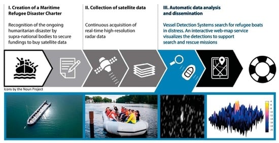
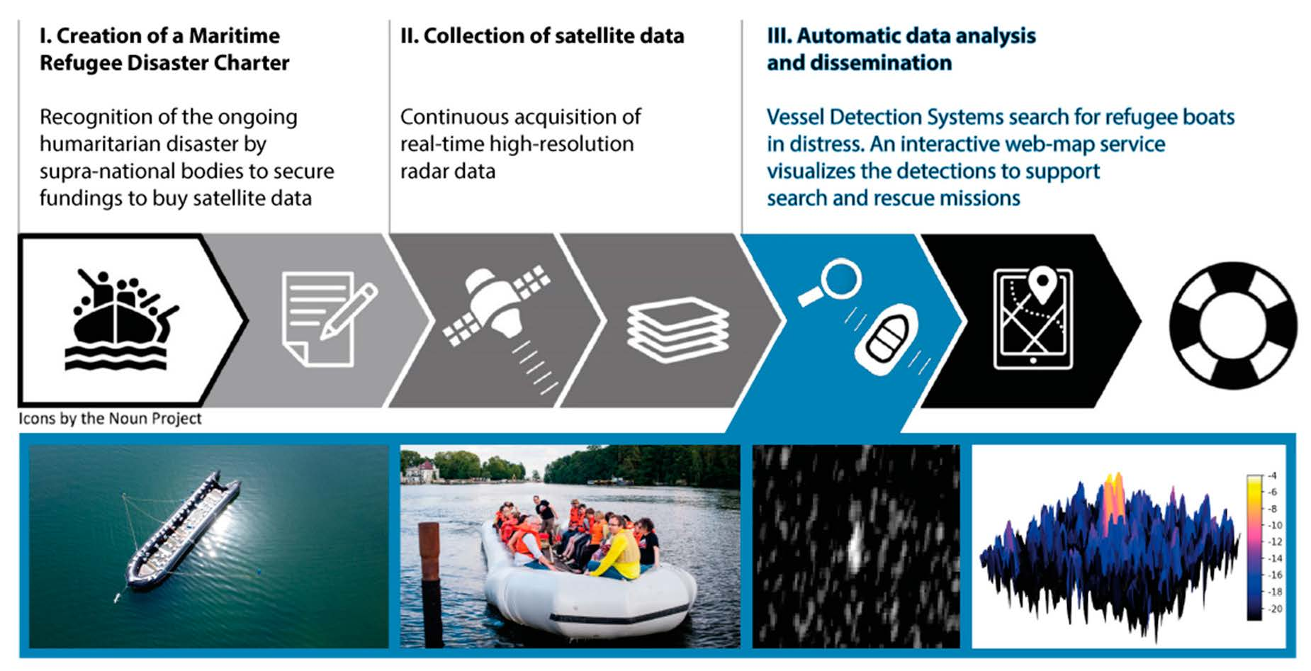
1. Introduction
2. Materials and Methods
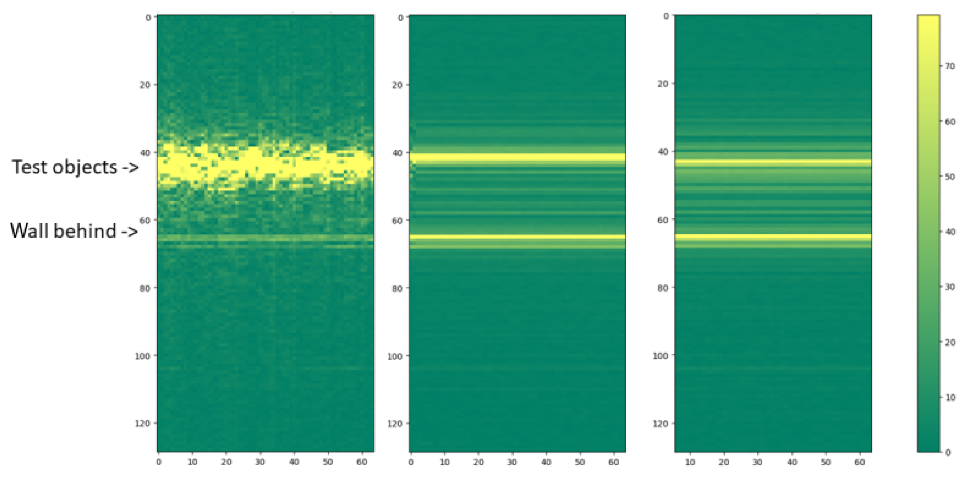
2.1. The Human Scattering Experiment
- Four volunteers sitting close to each other on the ground of an empty room. We chose the sitting posture because that most closely resembles the real situation in the migrant inflatable. The data include different arrangements: four people in a row perpendicular to the sensor line of sight (LoS) (‘H4×1’), two rows of two people behind each other (‘H2×2’) and all four people in one column behind each other parallel to the LoS (‘H1×4’).
- Water-soaked clay pebbles, packed in 30 × 40 cm air-tight plastic bags. The bags themselves are invisible to microwaves and the soaked clay pebbles, as they are roundish objects smaller than the wavelength and with a similar water content to the human body and, thus, should appear similar to the uppermost body parts (heads and shoulders). We took data from two bags perpendicular to the LoS (‘C2×1’), two bags parallel to the LoS (‘C1×2’), two bags sitting on top of each other (‘C1×1×2’) and two bags stacked with one large bag ( 30 × 60 cm) standing behind them (‘C1×1×2+1’).
- Steel wool clumped to random 20 cm diameter balls to imitate the top layer of passengers in a boat. The acquisitions involved six balls in two rows (‘S2×3’) and two balls plus four 5 × 10 × 60 cm (h,w,l) steel wool layers not clumped but stretched out in the front (‘S2+4’).
2.2. Data Campaign and Data Collection
- Cross-wind waves: these are waves that move perpendicular to the LoS. They move in the direction of the satellite azimuth, which is close to N-S.
- Up/down-wind waves: here, the waves move in the range direction.
- North Sea: Atlantic–European North-West Shelf-Wave Physics Reanalysis.
- Mediterranean Sea and West Gibraltar region: Mediterranean Sea Waves Reanalysis.
- Arctic Ocean: Arctic Ocean Wave Hindcast.
- All other maritime regions not covered by a high-resolution wave model: Global Ocean Waves Reanalysis WAVERYS.
2.3. Polarimetric Analysis of the Inflatable
2.4. Detector Comparison and Detector Fusion
3. Results
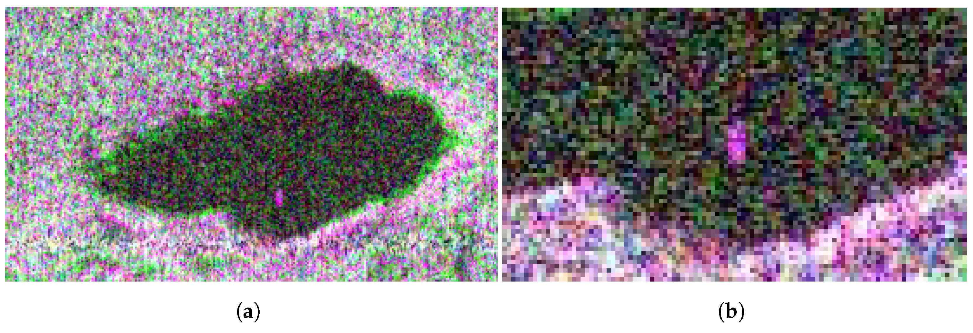
3.1. Qualitative Inspection of High Resolution Data
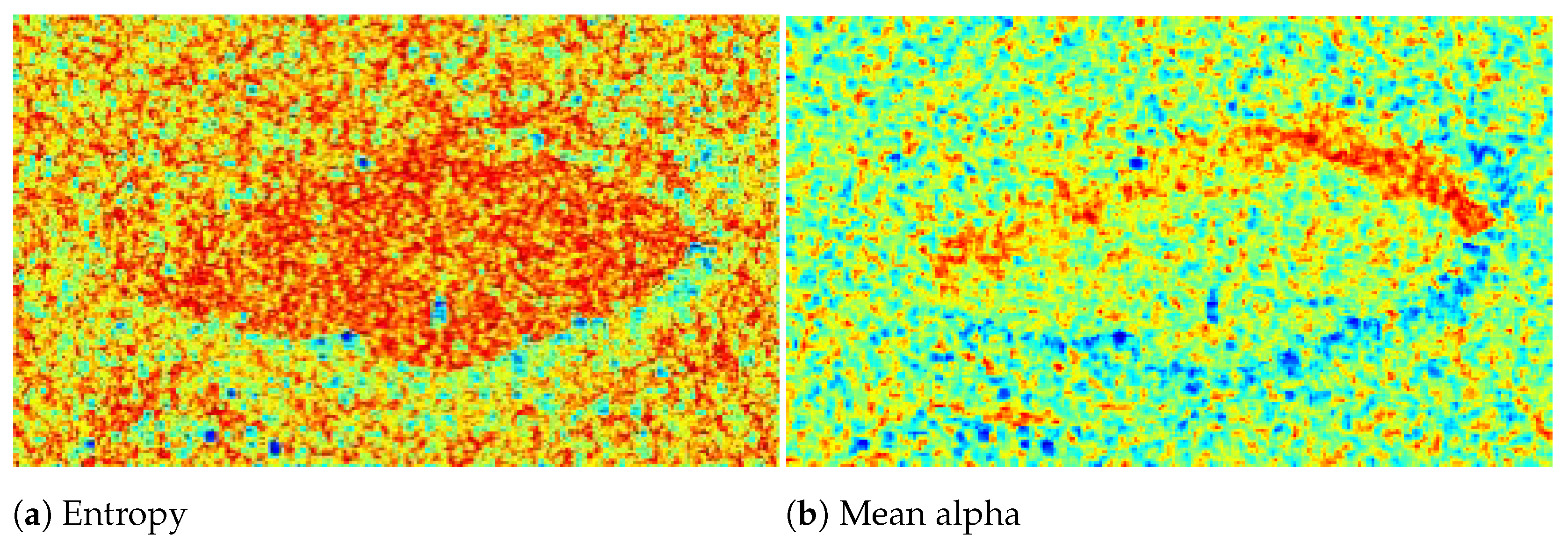
3.2. Polarimetric Scattering Analysis
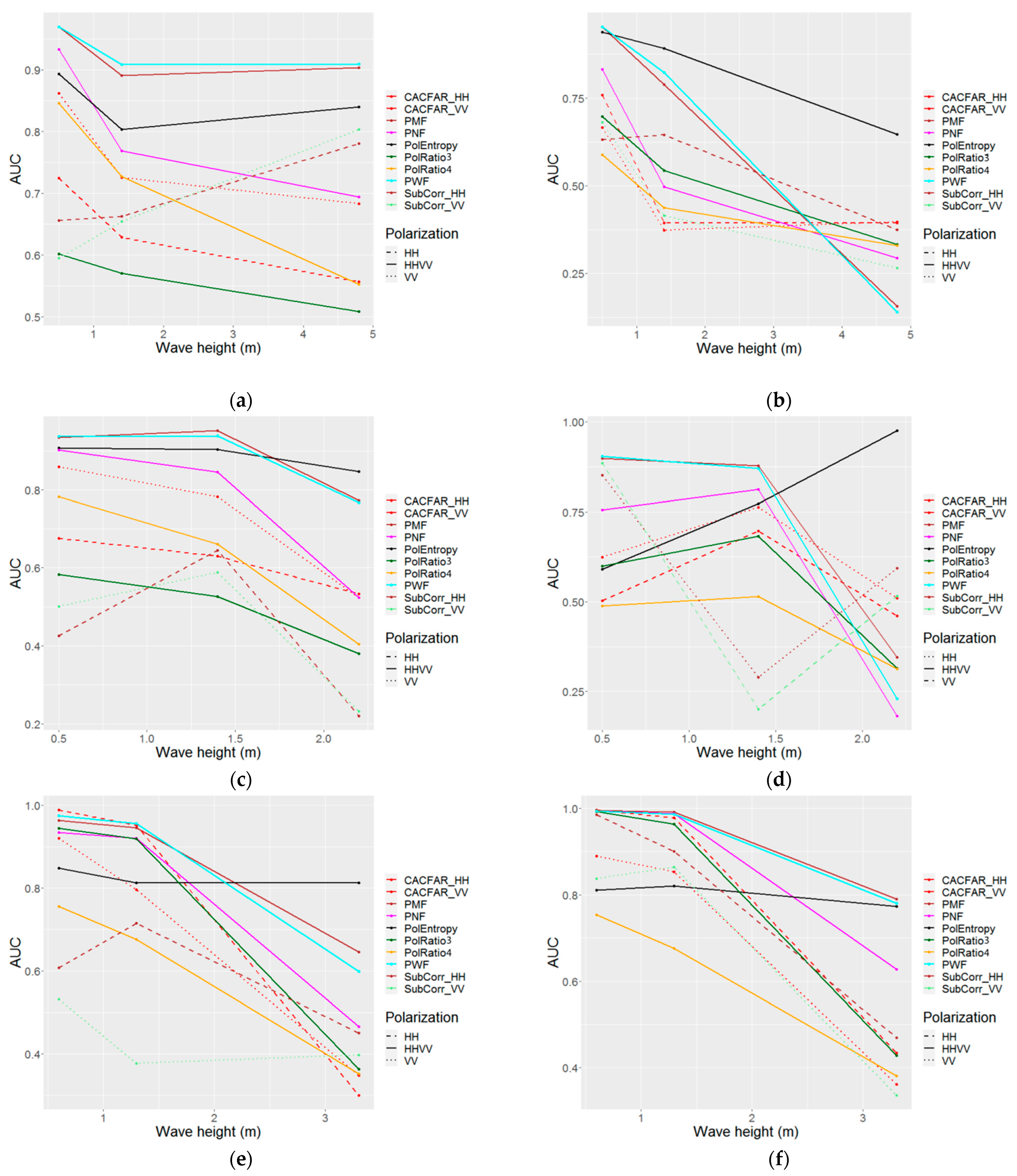
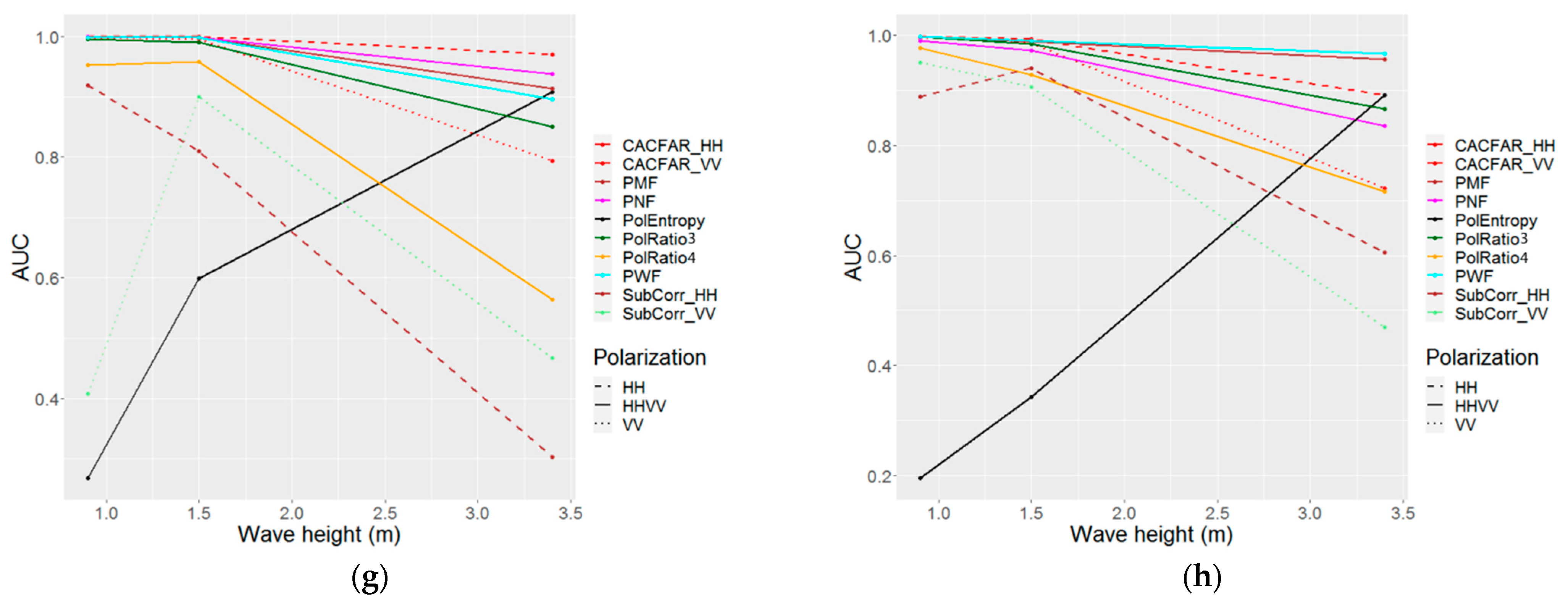
3.3. Detector Testing
- HH VV: the water surface has lower entropy values than the boat except for low sea states and/or high incidence angles.
- HV HH: medium angles: the entropy of the water stays higher than that of the boat; high angles: the entropy of water stays higher than that of the boat.
- VH VV: the entropy of water is lower than that of the boat.
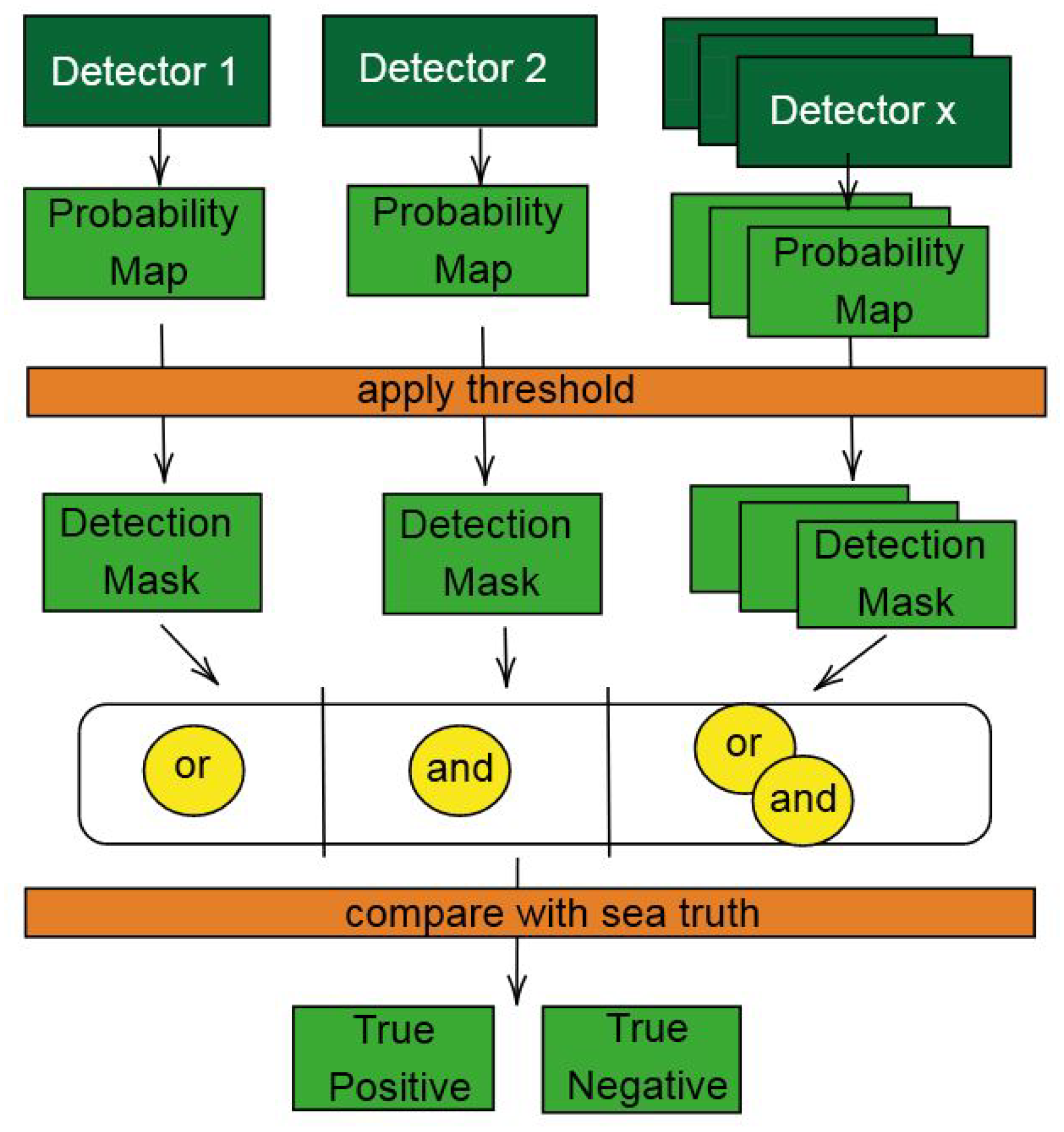
3.4. Detector Fusion
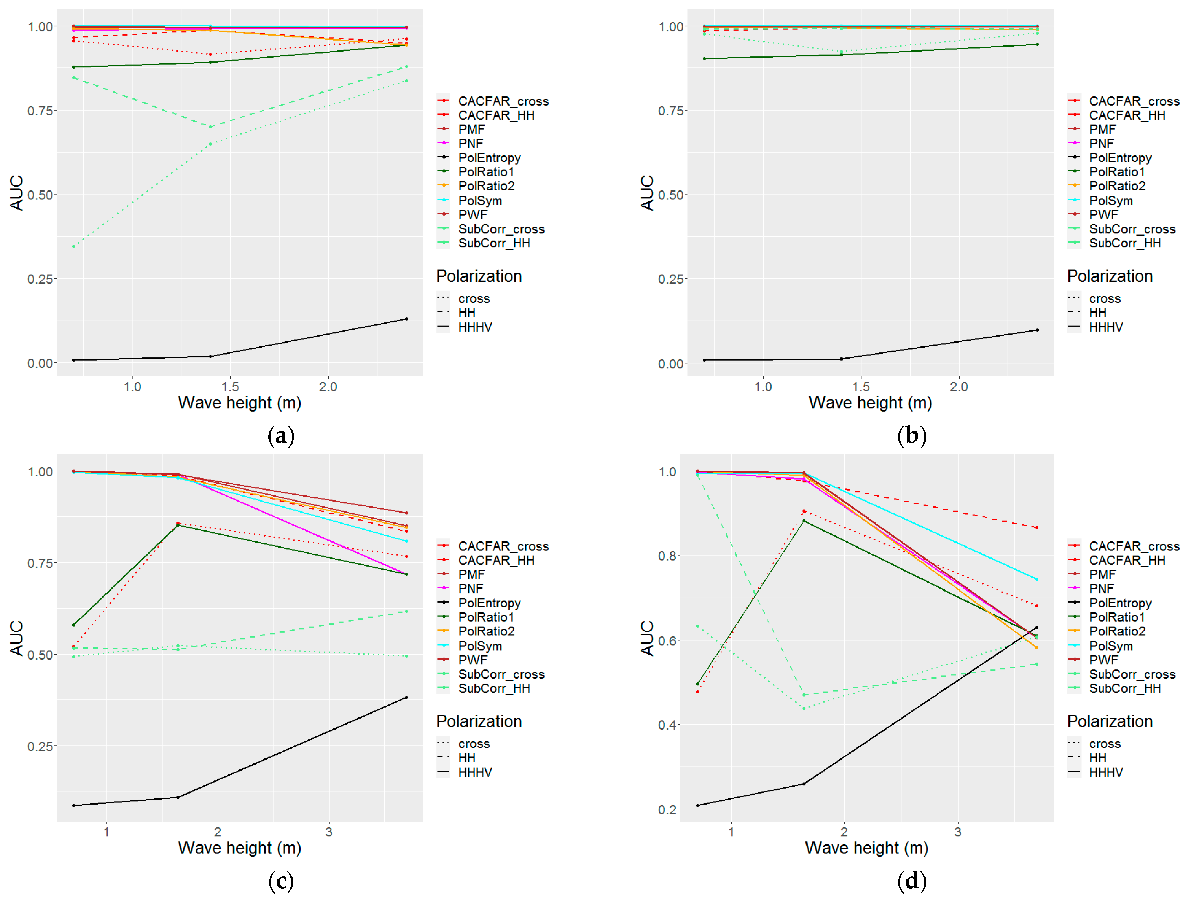
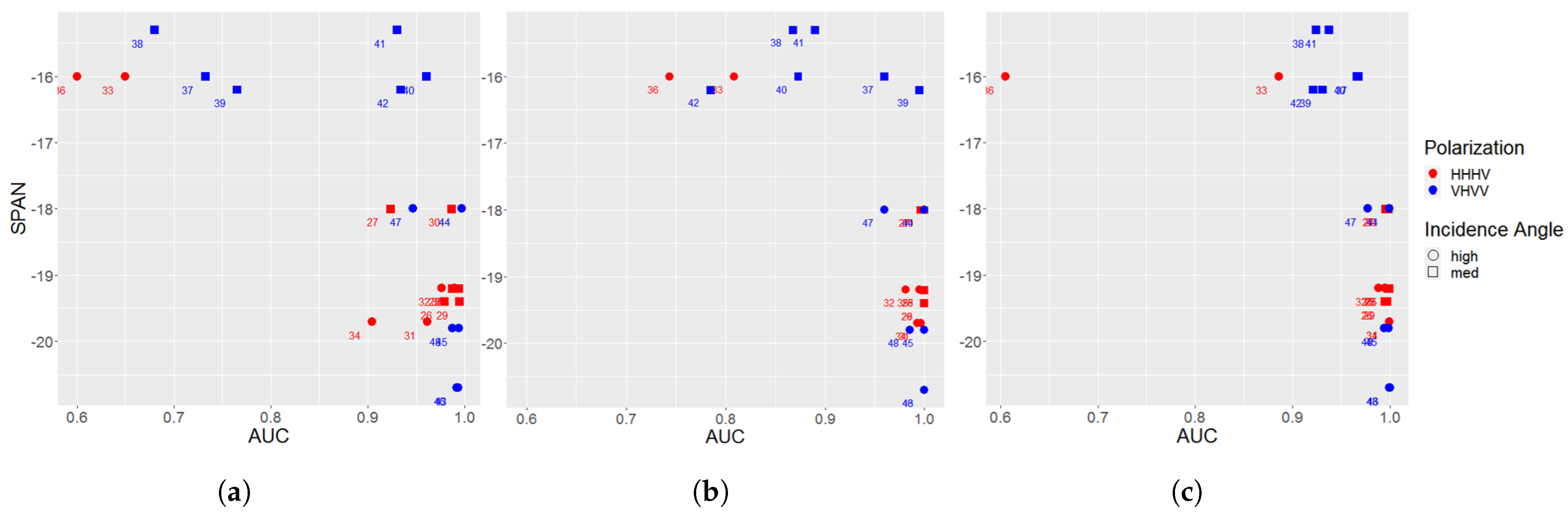
3.5. Estimation of the Detection Quality
4. Discussion
- The resolution was high enough to resolve the boat pixels separately from the ocean to a large extent.
- The interactions between the vessel and the water surface (flattening of the water surface below the vessel and those caused by the wind shadow on the lee side) were the same in our simulation and in the real situation.
- The wetness of the boat (salty spray on the inflatable and water inside the boat were the same in our simulation and in the real situation.
5. Conclusions
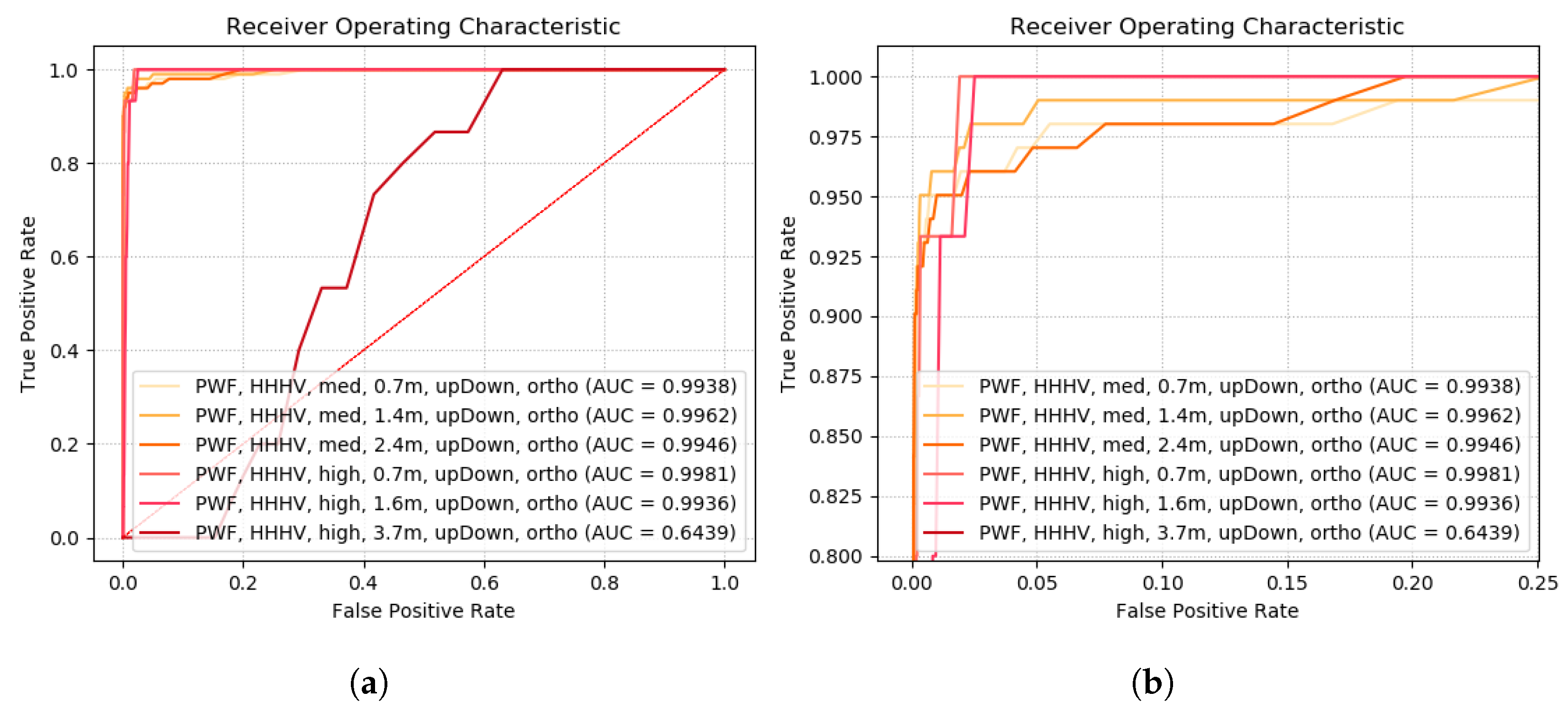
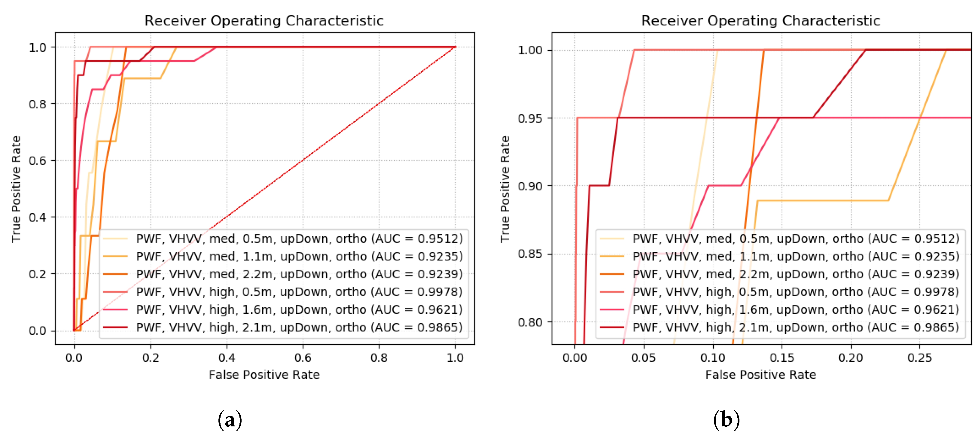
- With dual cross-pol channel combinations, the polarimetric whitening filter (PWF) was the best-performing detector.
- With HV HH, the PWF reached, at medium incidence angles, a detection rate of 90% with only 0.12% false detections. Our data support the assumption that the PWF can be used up to a maximum wave height of about 2.4 metres.
- With VH VV data, the PWF had a false detection rate of 1.07% at a 90% detection rate and up to 2.1 m wave height.
- For dual co-pol data, the HT22AND was the best detection algorithm with a false alarm rate of 0.59% at a detection rate of 90%. This is true for wave heights of up to 1.5 m and medium or high incidence angles.
Author Contributions
Funding
Informed Consent Statement
Data Availability Statement
Acknowledgments
Conflicts of Interest
References
- IOM. Missing Migrants Project. Available online: https://missingmigrants.iom.int/region/mediterranean (accessed on 23 March 2023).
- IOM. Displacement Tracking Matrix. Available online: https://dtm.iom.int/europe/arrivals (accessed on 23 March 2023).
- UNHCR. Mediterranean Situation. Available online: https://data.unhcr.org/en/situations/mediterranean (accessed on 23 March 2023).
- Novak, L.M.; Sechtin, M.B.; Burl, M.C. Algorithms for Optimal Processing of Polarimetric Radar Data; Polarimetric Technology Handbook, GACIAC HB 92–01, 139–206, Chicago; Massachusetts Institute of Technology Lexington Lincoln Lab: Lexington, MA, USA, 1989; p. 99. [Google Scholar]
- Crisp, D.J.; Redding, N.J. Ship Detection in Synthetic Aperture Radar Imagery. In Proceedings of the 12th Australasian Remote Sensing and Photogrammetry Conference, Fremantle, Australia, 18–22 October 2004; p. 10. [Google Scholar]
- Liu, C.; Vachon, P.W.; Geling, G.W. Improved Ship Detection Using Polarimetric SAR Data. In Proceedings of the IGARSS 2004, 2004 IEEE International Geoscience and Remote Sensing Symposium, Anchorage, AK, USA, 20–24 September 2004; Volume 3, pp. 1800–1803. [Google Scholar] [CrossRef]
- Yeremy, M.; Campbell, J.W.M.; Mattar, K.; Potter, T. Ocean Surveillance with Polarimetric SAR. Can. J. Remote Sens. 2001, 27, 328–344. [Google Scholar] [CrossRef]
- Touzi, R.; Charbonneau, F.; Hawkins, R.K.; Murnaghan, K.; Kavoun, X. Ship-Sea Contrast Optimization When Using Polarimetric SARs. In Proceedings of the IGARSS 2001, Scanning the Present and Resolving the Future, Proceedings, IEEE 2001 International Geoscience and Remote Sensing Symposium (Cat. No. 01CH37217), Sydney, Australia, 9–13 July 2001; Volume 1, pp. 426–428. [Google Scholar]
- Marino, A. A Notch Filter for Ship Detection with Polarimetric SAR Data. IEEE J. Sel. Top. Appl. Earth Obs. Remote Sens. 2013, 6, 1219–1232. [Google Scholar] [CrossRef]
- Marino, A.; Sugimoto, M.; Nunziata, F.; Hajnsek, I.; Migliaccio, M.; Ouchi, K. Comparison of Ship Detectors Using Polarimetric Alos Data: Tokyo Bay. In Proceedings of the 2013 IEEE International Geoscience and Remote Sensing Symposium (IGARSS), Melbourne, Australia, 21–26 July 2013; pp. 2345–2348. [Google Scholar]
- Nunziata, F.; Migliaccio, M.; Brown, C.E. Reflection Symmetry for Polarimetric Observation of Man-Made Metallic Targets at Sea. IEEE J. Ocean. Eng. 2012, 37, 384–394. [Google Scholar] [CrossRef]
- Kang, M.; Ji, K.; Leng, X.; Lin, Z. Contextual Region-Based Convolutional Neural Network with Multilayer Fusion for SAR Ship Detection. Remote Sens. 2017, 9, 860. [Google Scholar] [CrossRef]
- Zhao, J.; Guo, W.; Zhang, Z.; Yu, W. A Coupled Convolutional Neural Network for Small and Densely Clustered Ship Detection in SAR Images. Sci. China Inf. Sci. 2019, 62, 42301. [Google Scholar] [CrossRef]
- Girshick, R.; Donahue, J.; Darrell, T.; Malik, J. Rich Feature Hierarchies for Accurate Object Detection and Semantic Segmentation. In Proceedings of the 2014 IEEE Conference on Computer Vision and Pattern Recognition, Columbus, OH, USA, 23–28 June 2014; pp. 580–587. [Google Scholar] [CrossRef]
- Girshick, R. Fast R-Cnn. In Proceedings of the IEEE International Conference on Computer Vision, Santiago, Chile, 7–13 December 2015; pp. 1440–1448. [Google Scholar]
- Ren, S.; He, K.; Girshick, R.; Sun, J. Faster R-CNN: Towards Real-Time Object Detection with Region Proposal Networks. In Advances in Neural Information Processing Systems 28; Cortes, C., Lawrence, N.D., Lee, D.D., Sugiyama, M., Garnett, R., Eds.; Curran Associates, Inc.: Red Hook, NY, USA, 2015; pp. 91–99. [Google Scholar]
- Li, J.; Qu, C.; Shao, J. Ship Detection in SAR Images Based on an Improved Faster R-CNN. In Proceedings of the 2017 SAR in Big Data Era: Models, Methods and Applications (BIGSARDATA), Beijing, China, 13–14 November 2017; pp. 1–6. [Google Scholar] [CrossRef]
- Zhang, S.; Wu, R.; Xu, K.; Wang, J.; Sun, W. R-CNN-Based Ship Detection from High Resolution Remote Sensing Imagery. Remote Sens. 2019, 11, 631. [Google Scholar] [CrossRef]
- Zhang, T.; Zhang, X. High-Speed Ship Detection in SAR Images Based on a Grid Convolutional Neural Network. Remote Sens. 2019, 11, 1206. [Google Scholar] [CrossRef]
- Redmon, J.; Divvala, S.; Girshick, R.; Farhadi, A. You Only Look Once: Unified, Real-Time Object Detection. In Proceedings of the 2016 IEEE Conference on Computer Vision and Pattern Recognition (CVPR), Las Vegas, NV, USA, 27–30 June 2016; pp. 779–788. [Google Scholar] [CrossRef]
- Chang, Y.L.; Anagaw, A.; Chang, L.; Wang, Y.; Hsiao, C.Y.; Lee, W.H. Ship Detection Based on YOLOv2 for SAR Imagery. Remote Sens. 2019, 11, 786. [Google Scholar] [CrossRef]
- Rostami, M.; Kolouri, S.; Eaton, E.; Kim, K. Deep Transfer Learning for Few-Shot SAR Image Classification. Remote Sens. 2019, 11, 1374. [Google Scholar] [CrossRef]
- Lanz, P.; Marino, A.; Brinkhoff, T.; Köster, F.; Möller, M. The InflateSAR Campaign: Evaluating SAR Identification Capabilities of Distressed Refugee Boats. Remote Sens. 2020, 12, 3516. [Google Scholar] [CrossRef]
- Lanz, P.; Marino, A.; Brinkhoff, T.; Köster, F.; Möller, M. The InflateSAR Campaign: Testing SAR Vessel Detection Systems for Refugee Rubber Inflatables. Remote Sens. 2021, 13, 1487. [Google Scholar] [CrossRef]
- Marino, A.; Dierking, W.; Wesche, C. A Depolarization Ratio Anomaly Detector to Identify Icebergs in Sea Ice Using Dual-Polarization SAR Images. IEEE Trans. Geosci. Remote Sens. 2016, 54, 5602–5615. [Google Scholar] [CrossRef]
- Holt, B. SAR Imaging of the Ocean Surface. In Synthetic Aperture Radar Marine User’s Manual; Jackson, C., Apel, J., Eds.; NOAA/NESDIS: Washington, DC, USA, 2004; pp. 25–79. [Google Scholar]
- Microwaves101. Miscellaneous Dielectric Constants. Available online: https://www.microwaves101.com/encyclopedias/miscellaneous-dielectric-constants (accessed on 15 January 2023).
- Agency, E.S. Mediterranean Sea Salinity. Available online: https://www.esa.int/ESA_Multimedia/Images/2017/05/Mediterranean_Sea_salinity (accessed on 17 January 2023).
- Van Zyl, J.J.; Arii, M.; Kim, Y. Model-Based Decomposition of Polarimetric SAR Covariance Matrices Constrained for Nonnegative Eigenvalues. IEEE Trans. Geosci. Remote Sens. 2011, 49, 3452–3459. [Google Scholar] [CrossRef]
- Klein, L.A.; Swift, C.T. An Improved Model for the Dielectric Constant of Sea Water at Microwave Frequencies. IEEE Trans. Antennas Propag. 1977, 25, 104–111. [Google Scholar] [CrossRef]
- Guo, C.; Ye, H.; Zhou, Y.; Xu, Y.; Wang, L. Scaled Sea Surface Design and RCS Measurement Based on Rough Film Medium. Sensors 2022, 22, 6290. [Google Scholar] [CrossRef] [PubMed]
- Hozhabri, M.; Risman, P.O.; Petrovic, N. Comparison of UWB Radar Backscattering by the Human Torso and a Phantom. In Proceedings of the 2018 IEEE Conference on Antenna Measurements & Applications (CAMA), Västerås, Sweden, 3–6 September 2018; pp. 1–4. [Google Scholar] [CrossRef]
- Valenzuela, G.R. Theories for the Interaction of Electromagnetic and Oceanic Waves—A Review. Bound.-Layer Meteorol. 1978, 13, 61–85. [Google Scholar] [CrossRef]
- Robinson, I.S. Measuring the Oceans from Space: The Principles and Methods of Satellite Oceanography; Springer Science & Business Media: Berlin/Heidelberg, Germany, 2004. [Google Scholar]
- Voronovich, A.G.; Zavorotny, V.U. Theoretical Model for Scattering of Radar Signals in Ku- and C-bands from a Rough Sea Surface with Breaking Waves. Waves Random Media 2001, 11, 247. [Google Scholar] [CrossRef]
- Mouche, A.A.; Chapron, B.; Reul, N. A Simplified Asymptotic Theory for Ocean Surface Electromagnetic Wave Scattering. Waves Random Complex Media 2007, 17, 321–341. [Google Scholar] [CrossRef]
- Kudryavtsev, V.; Hauser, D.; Caudal, G.; Chapron, B. A Semiempirical Model of the Normalized Radar Cross-Section of the Sea Surface 1. Background Model. J. Geophys. Res. Ocean. 2003, 108, FET 2-1–FET 2-24. [Google Scholar] [CrossRef]
- Ren, Y.; Lehner, S.; Brusch, S.; Li, X.; He, M. An Algorithm for the Retrieval of Sea Surface Wind Fields Using X-band TerraSAR-X Data. Int. J. Remote Sens. 2012, 33, 7310–7336. [Google Scholar] [CrossRef]
- Weber, J.E.H. Vertically Varying Eulerian Mean Currents Induced by Internal Coastal Kelvin Waves. J. Geophys. Res. Ocean. 2017, 122, 1222–1231. [Google Scholar] [CrossRef]
- Zhang, L.; Zhang, J.; Zou, B.; Zhang, Y. Comparison of Methods for Target Detection and Applications Using Polarimetric SAR Image. In Proceedings of the Progress in Electromagnetics Research Symposium, Hangzhou, China, 24–28 March 2008; Volume 1. [Google Scholar]
- Cloude, S.R.; Pottier, E. A Review of Target Decomposition Theorems in Radar Polarimetry. IEEE Trans. Geosci. Remote Sens. 1996, 34, 498–518. [Google Scholar] [CrossRef]
- Cloude, S.; Pottier, E. An Entropy Based Classication Scheme for Land Applications of Polarimetric SAR. IEEE Trans. Geosci. Remote Sens. 1997, 35, 68–78. [Google Scholar] [CrossRef]
- Yamaguchi, Y.; Moriyama, T.; Ishido, M.; Yamada, H. Four-Component Scattering Model for Polarimetric SAR Image Decomposition. IEEE Trans. Geosci. Remote Sens. 2005, 43, 1699–1706. [Google Scholar] [CrossRef]
- Freeman, A.; Durden, S.L. Three-Component Scattering Model to Describe Polarimetric SAR Data. In Proceedings of the Radar Polarimetry; International Society for Optics and Photonics: Washington, DC, USA, 1993; Volume 1748, pp. 213–224. [Google Scholar]
- Kennaugh, E.M.; Sloan, R.W. Effects of Type of Polarization On Echo Characteristics; Technical Report; Ohio State Univ Research Foundation Columbus Antenna Lab: Columbus, OH, USA, 1952. [Google Scholar]
- Cameron, W.L.; Leung, L.K. Feature Motivated Polarization Scattering Matrix Decomposition. In Proceedings of the IEEE International Conference on Radar, Arlington, VA, USA, 7–10 May 1990; pp. 549–557. [Google Scholar]
- Krogager, E. New Decomposition of the Radar Target Scattering Matrix. Electron. Lett. 1990, 26, 1525–1527. [Google Scholar] [CrossRef]
- Karachristos, K.; Anastassopoulos, V. Land Cover Classification Based on Double Scatterer Model and Neural Networks. Geomatics 2022, 2, 323–337. [Google Scholar] [CrossRef]
- Singh, G.; Mohanty, S.; Yamazaki, Y.; Yamaguchi, Y. Physical Scattering Interpretation of POLSAR Coherency Matrix by Using Compound Scattering Phenomenon. IEEE Trans. Geosci. Remote Sens. 2020, 58, 2541–2556. [Google Scholar] [CrossRef]
- Tello, M.; López-Martínez, C.; Mallorqui, J.J. A Novel Algorithm for Ship Detection in SAR Imagery Based on the Wavelet Transform. IEEE Geosci. Remote Sens. Lett. 2005, 2, 201–205. [Google Scholar] [CrossRef]
- Raney, R.K. Synthetic Aperture Imaging Radar and Moving Targets. IEEE Trans. Aerosp. Electron. Syst. 1971, AES-7, 499–505. [Google Scholar] [CrossRef]


| Material | Dielectric Constant | Loss Tangent |
|---|---|---|
| Air | 1 | depends on weather |
| Blood * | 58 | 0.27 |
| Fat * | 5.5 | 0.21 |
| Muscle * | 49 | 0.33 |
| Nylon | 2.4 | 0.0083 |
| Polyethylene | 2.25 | - |
| Water, fresh [29] | 80 | - |
| Sea water [30,31] | 70 | - |
| Sea ice [26] | 4 | 0.5 |
| Sandy soil (dry) | 2.55 | 0.0062 |
| Clay bricks | 3.7–4.5 | - |
| Metals | infinite | - |
| Plywood | 2.5 |
| Mission | Mode | Average Pixel Size (m²) | Polarization | Incidence Angle | Datasets |
|---|---|---|---|---|---|
| TerraSAR-X | Stripmap | 4.4 | Dual-pol: HH VV, HV HH, VH VV | Low, medium and high | 46 |
| Cosmo- SkyMed | Spotlight | 2.7 | Quad-Pol | Medium and high | 4 |
| ICEYE | High-res. Spotlight | 0.6 | Single-Pol: VV | Low and medium | 4 |
| 90 Degrees | 45 Degrees | |||||
|---|---|---|---|---|---|---|
| Low | Medium | High | Low | Medium | High | |
| HH VV | 1 (1) | 4 | 3 | 3 (2) | 5 | 5 |
| HV HH | 1 | 2 | 2 | 1 (1) | 3 | 2 |
| VH VV | 1 | 2 | 1 | 1 (1) | 2 | 2 |
| Polarization | HH VV | HV HH | VH VV | |||||
|---|---|---|---|---|---|---|---|---|
| Incidence Angle | Low | Low | Medium | High | Medium | High | Medium | High |
| Wave Direction | Cross | Up/Down | Up/Down | Up/Down | Up/Down | Up/Down | Up/Down | Up/Down |
| Wave Height (m) | ||||||||
| 0.4–0.8 (BFT3) | ✓ | ✓ | ✓ | ✓ | ✓ | ✓ | ✓ | ✓ |
| 0.8–1.5 (BFT4) | ✓ | ✓ | ✓ | ✓ | ✓ | ✓ | ✓ | |
| 1.5–2.5 (BFT5) | ✓ | ✓ | ✓ | ✓ | ✓ | |||
| 2.5–3.5 (BFT6) | ✓ | ✓ | ||||||
| 3.5–4.5 (BFT7) | ✓ | |||||||
| 4.5–6.5 (BFT8) | ✓ | |||||||
| Parameter | Decomposition | Note |
|---|---|---|
| Alpha | Cloude–Pottier | |
| Entropy | Cloude–Pottier | |
| Single Bounce | Yamaguchi Y4R | |
| Double Bounce | Yamaguchi Y4R | |
| Volume Scattering | Yamaguchi Y4R | |
| Helix Scattering | Yamaguchi Y4R | |
| Symmetry | Yamaguchi Y4R | Huynen Target Generator A0 |
| Irregularity/Double Bounce | Yamaguchi Y4R | Huynen Target Generator B0-B |
| Non-symmetry | Yamaguchi Y4R | Huynen Target Generator B0+B |
| Even bounce | Pauli | |HH-VV| |
| Even bounce 45° oriented | Pauli | |HV| |
| Odd bounce | Pauli | |HH+VV| |
| Trihedral | Cameron | |
| Dipole | Cameron | |
| Narrow Diplane | Cameron | |
| Diplane | Cameron | |
| Left Helix | Cameron | |
| Right Helix | Cameron | |
| Cylinder | Cameron | |
| 1/4 Wave Device | Cameron |
| Detector | Cells Under Test (CUT) Window Size | Guard Window Size | Train Window Size |
|---|---|---|---|
| Polarimetric Symmetry Detector (PolSym) | 1 | 2 | 5 |
| Polarimetric Notch Filter (PNF) | 5 | 12 | 36 |
| Polarimetric Entropy Detector (PolEntropy) | 2 | - | 10 |
| Polarimetric Match Filter (PMF) | 5 | 12 | 36 |
| Intensity Depolarization Ratio Anomaly Detector (iDPolRAD) | 1 | 12 | 36 |
| Surface Intensity Depolarization Ratio Anomaly Detector (SiDPolRAD) | 1 | 12 | 36 |
| Sub-look Correlation Detector (SubCorr) | 1 | - | 36 |
| Polarimetric Whitening Filter (PWF) | 5 | 12 | 36 |
| Cell Averaging Constant False Alarm Rate (CA-CFAR) | 1 | 24 | 36 |
| Double Bounce | Volume | Single Bounce | |
|---|---|---|---|
| low inc. angle, inclined vessel | 0.41 | 0.25 | 0.41 |
| low inc. angle, orthogonal vessel | 0.33 | 0.17 | 0.33 |
| medium inc. angle, orthogonal vessel | 0.68 | 0.26 | 0.73 |
| H | Mean Alpha | |
|---|---|---|
| Low inc. angle, inclined vessel | 0.46 | 0.32 |
| Low inc. angle, orthogonal vessel | 0.46 | 0.65 |
| Medium inc. angle, orthogonal vessel | 0.58 | 0.54 |
| Helix | Single Bounce | Volume | Double Bounce | |
|---|---|---|---|---|
| Low inc. angle, inclined vessel | 0.00 | 0.07 | 0.01 | 0.49 |
| Low inc. angle, orthogonal vessel | 0.00 | 0.48 | 0.01 | 0.00 |
| Medium inc. angle, orthogonal vessel | 0.00 | 0.80 | 0.01 | 0.39 |
| Trihedral | Dipole | Narrow Diplane | Diplane | Cylinder | 1/4 Wave Device | Left Helix | Right Helix | |
|---|---|---|---|---|---|---|---|---|
| low inc. angle, inclined vessel | 0.08 | 0.47 | 0.17 | 0.07 | 0.26 | 0.18 | 0.03 | 0.01 |
| low inc. angle, orthogonal vessel | 0.15 | 0.53 | 0.22 | 0.06 | 0.11 | 0.21 | 0.02 | 0.01 |
| medium inc. angle, orthogonal vessel | 0.06 | 0.57 | 0.15 | 0.06 | 0.23 | 0.10 | 0.00 | 0.00 |
| Polarization | HH VV | HV HH | VH VV | |||||
|---|---|---|---|---|---|---|---|---|
| Incidence Angle | Low | Medium | High | Medium | High | Medium | High | Avg |
| PMF | 0.787 | 0.888 | 0.976 | 0.996 | 0.906 | 0.945 | 0.995 | 0.928 |
| PWF | 0.779 | 0.882 | 0.975 | 0.997 | 0.912 | 0.941 | 0.995 | 0.926 |
| PNF | 0.67 | 0.822 | 0.956 | 0.994 | 0.881 | 0.871 | 0.986 | 0.883 |
| PolEntropy | 0.834 | 0.813 | 0.534 | 0.046 | 0.279 | 0.559 | 0.373 | 0.491 |
| PolRatio1/3 | 0.529 | 0.768 | 0.947 | 0.913 | 0.689 | 0.714 | 0.939 | 0.786 |
| PolRatio2/4 | 0.554 | 0.599 | 0.849 | 0.983 | 0.9 | 0.768 | 0.936 | 0.799 |
| SubCorr_HH | 0.565 | 0.688 | 0.744 | 0.9 | 0.608 | 0.701 | ||
| SubCorr_VV | 0.528 | 0.557 | 0.684 | 0.604 | 0.481 | 0.571 | ||
| SubCorr_cross | 0.785 | 0.531 | 0.483 | 0.537 | 0.584 | |||
| CACFAR_HH | 0.6 | 0.775 | 0.975 | 0.98 | 0.943 | 0.854 | ||
| CACFAR_VV | 0.628 | 0.695 | 0.915 | 0.798 | 0.946 | 0.797 | ||
| CACFAR_cross | 0.972 | 0.701 | 0.766 | 0.909 | 0.837 | |||
| PolSym | 0.999 | 0.92 | 0.895 | 0.991 | 0.951 | |||
| avg | 0.647 | 0.749 | 0.856 | 0.869 | 0.752 | 0.759 | 0.826 | |
| Polarization | HH VV | HV HH | VH VV | |||||
|---|---|---|---|---|---|---|---|---|
| Incidence Angle | Low | Medium | High | Medium | High | Medium | High | Avg |
| PMF | 0.787 | 0.843 | 0.935 | 0.728 | 0.945 | 0.848 | ||
| PWF | 0.779 | 0.83 | 0.932 | 0.745 | 0.941 | 0.846 | ||
| PNF | 0.67 | 0.75 | 0.887 | 0.662 | 0.871 | 0.768 | ||
| PolEntropy | 0.834 | 0.804 | 0.9 | 0.506 | 0.559 | 0.721 | ||
| PolRatio1/3 | 0.529 | 0.669 | 0.858 | 0.664 | 0.714 | 0.687 | ||
| PolRatio2/4 | 0.554 | 0.521 | 0.64 | 0.714 | 0.768 | 0.639 | ||
| SubCorr_HH | 0.565 | 0.634 | 0.455 | 0.58 | 0.558 | |||
| SubCorr_VV | 0.528 | 0.494 | 0.468 | 0.604 | 0.523 | |||
| SubCorr_cross | 0.551 | 0.483 | 0.517 | |||||
| CACFAR_HH | 0.6 | 0.666 | 0.931 | 0.85 | 0.762 | |||
| CACFAR_VV | 0.628 | 0.59 | 0.758 | 0.798 | 0.694 | |||
| CACFAR_cross | 0.723 | 0.766 | 0.745 | |||||
| PolSym | 0.776 | 0.895 | 0.835 | |||||
| avg | 0.647 | 0.68 | 0.776 | 0.682 | 0.759 | |||
| Polarization | HH VV | HV HH | VH VV | |||||
|---|---|---|---|---|---|---|---|---|
| Incidence Angle | Low | Medium | High | Medium | High | Medium | High | Avg |
| PMF | 0.23 | −0.07 | −0.01 | 0 | 0.08 | 0 | 0.01 | 0.03 |
| PWF | 0.25 | −0.08 | −0.02 | 0 | 0.09 | 0 | 0.01 | 0.04 |
| PNF | 0.22 | −0.10 | 0.05 | −0.01 | 0.04 | 0.08 | 0.02 | 0.04 |
| PolEntropy | 0.06 | 0.02 | 0.12 | 0.01 | −0.17 | 0.51 | −0.50 | 0.01 |
| PolRatio1/3 | 0 | −0.05 | 0 | −0.02 | 0.05 | 0.44 | 0.1 | 0.07 |
| PolRatio2/4 | 0.22 | −0.01 | −0.05 | −0.02 | 0.09 | −0.35 | 0.12 | 0 |
| SubCorr_HH | 0 | −0.19 | −0.13 | −0.18 | −0.12 | −0.13 | ||
| SubCorr_VV | 0.07 | −0.24 | −0.18 | −0.26 | 0.3 | −0.06 | ||
| SubCorr_cross | −0.35 | −0.06 | 0.15 | −0.09 | −0.09 | |||
| CACFAR_HH | 0.05 | −0.06 | 0.03 | −0.03 | −0.01 | 0 | ||
| CACFAR_VV | 0.22 | −0.01 | 0.03 | −0.20 | 0.09 | 0.03 | ||
| CACFAR_cross | −0.06 | 0.03 | 0.46 | 0.14 | 0.14 | |||
| PolSym | 0 | 0.02 | 0.09 | 0.02 | 0.03 | |||
| avg | 0.13 | −0.08 | −0.02 | −0.06 | 0 | 0.08 | 0.02 | 0.01 |
Disclaimer/Publisher’s Note: The statements, opinions and data contained in all publications are solely those of the individual author(s) and contributor(s) and not of MDPI and/or the editor(s). MDPI and/or the editor(s) disclaim responsibility for any injury to people or property resulting from any ideas, methods, instructions or products referred to in the content. |
© 2023 by the authors. Licensee MDPI, Basel, Switzerland. This article is an open access article distributed under the terms and conditions of the Creative Commons Attribution (CC BY) license (https://creativecommons.org/licenses/by/4.0/).
Share and Cite
Lanz, P.; Marino, A.; Simpson, M.D.; Brinkhoff, T.; Köster, F.; Möller, M. The InflateSAR Campaign: Developing Refugee Vessel Detection Capabilities with Polarimetric SAR. Remote Sens. 2023, 15, 2008. https://doi.org/10.3390/rs15082008
Lanz P, Marino A, Simpson MD, Brinkhoff T, Köster F, Möller M. The InflateSAR Campaign: Developing Refugee Vessel Detection Capabilities with Polarimetric SAR. Remote Sensing. 2023; 15(8):2008. https://doi.org/10.3390/rs15082008
Chicago/Turabian StyleLanz, Peter, Armando Marino, Morgan David Simpson, Thomas Brinkhoff, Frank Köster, and Matthias Möller. 2023. "The InflateSAR Campaign: Developing Refugee Vessel Detection Capabilities with Polarimetric SAR" Remote Sensing 15, no. 8: 2008. https://doi.org/10.3390/rs15082008