Article

On Evaluating the Predictability of Sea Surface Temperature Using Entropy

Department of Computer Science and Technology, Tongji University, Shanghai 201804, China
*
Author to whom correspondence should be addressed.
Remote Sens. 2023, 15(8), 1956; https://doi.org/10.3390/rs15081956
Submission received: 24 February 2023 / Revised: 5 April 2023 / Accepted: 5 April 2023 / Published: 7 April 2023

Abstract

:
Sea surface temperature (SST) has important impacts on the global ecology, and having a good understanding of the predictability, i.e., the possibility of achieving accurate prediction, of SST can help us monitor the marine environment and climate change, and guide the selection and design of SST prediction methods. However, existing studies for analyzing SST mostly measure the rising or falling trends of SST. To address this issue, we introduce a temporal-correlated entropy to quantify the predictability of SST series from both global coarse-grained and local fine-grained aspects, and make SST prediction with multiple deep learning models to prove the effectiveness of such predictability evaluation method. In addition, we explore the dynamics of SST predictability by dividing the time range of interest into consecutive time periods, evaluating the corresponding predictability of SST for each time period, and analyzing the stability of the predictability of SST over time. According to the experiments, the SST predictability values near the poles and equator are really high. The average SST predictability values of the East China Sea, Bohai Sea, and Antarctic Ocean are 0.719, 0.706, and 0.886, respectively, and the size relationship of the SST predictability in the three local sea areas is consistent with our prediction results using multiple representative SST prediction methods, which corroborates the reliability of the predictability evaluation method. In addition, we found that the SST predictability in the Antarctic Ocean changes more dramatically over time than in the East China Sea and the Bohai Sea. The results of SST predictability and its dynamic analysis indicate that global warming, ocean currents, and human activities all have significant impacts on the predictability of SST.

1. Introduction

The ocean covers about 71% of the Earth’s surface, and sea surface temperature(SST) is therefore of great importance for global climate and environment [1,2]. SST usually refers to the temperature of the seawater in the uppermost sea layer of 10–20 microns and at a depth from 1 mm to 20 m according to the varying measurement methods, including satellite and in situ sensors. SST is affected by many factors, such as ocean currents and sunlight, and presents certain temporal regularity. Therefore, having a good understanding of the predictability, i.e., regularity, of SST can help people better solve various issues in the ocean, e.g., SST prediction and marine climate analysis.
First, accurate SST prediction helps people cope with climate change and possible natural disasters in advance. Currently, various methods, e.g., physical models, time series methods, and machine learning models [3,4], have been proposed for SST prediction. These methods have different characteristics and perform quite differently at oceanic regions of different SST predictability. For example, time series methods usually achieve high accuracy in predicting SST of high predictability while performing badly if the predictability of SST is low. In contrast, machine learning methods could achieve higher prediction accuracy than time series methods for SST of low predictability because they can involve external data and knowledge to enrich the information for training prediction models. In this case, evaluating the predictability of SST can guide the selection and design of prediction models [5], and help to make more accurate SST predictions.
Second, global warming has been a prominent issue, and the melting of Antarctic and Arctic glaciers leads to the rapid rise of sea level [6], which seriously affects the global climate and ecological environment. Global warming leads to more climate anomalies, and causes drastic changes in SST in some ocean areas. Evaluating the predictability of SST and uncovering the dynamic changes in SST predictability can help to locate regions with drastic SST changes, making it possible to take some remedial actions in time. In addition, further analysis of the causes of SST changes could help us to find a specific and workable solution to global warming.
There are already many studies analyzing the dynamics of SST. Hansen et al. [7] measured the changes in global surface temperature and discovered that the Arctic Ocean has the largest warming amplitude. Bulgin et al. [8] quantified the global trends, variability, and persistence in SST and discussed the evidence for the re-emergence of sea surface temperature anomalies. Robles-Tamayo et al. [9] analyzed the SST time series to capture the oceanographic variability of the Eastern Coastal Zone of the Gulf of California. Li et al. [10] used linear regression to analyze the warming trend and seasonal change in the deep water in the Gulf of Mexico. Mohamed et al. [11] analyzed the temporal and spatial variation and linear trend of the SST in the Black Sea, and analyzed the interannual variation of SST using the empirical orthogonal function (EOF). Mohamed et al. [12] also studied the change in SST in the Barents Sea using the EOF method, and concluded that the Barents Sea has the greatest changes in SST in the Arctic. Hussein et al. [13] studied the correlations between chlorophyll-a and SST, and their trends in the Arabian Gulf. Zhao et al. [14] analyzed the spatial and temporal characteristics of SST in the North Pacific Ocean and the correlations between SST and other sea factors. In addition, there are also some studies analyzing the regularity of SST. Ba et al. [15] studied the regularity of ocean surface structure using satellite images in frontal regions in the ocean. Sutton et al. [16] used shipboard observations to analyze the decadal predictability of the SST in the North Atlantic. Davis [17] used EOF and linear statistical estimators to capture the variability of SST. However, all these existing studies above mainly focus on either analyzing the rising and falling trends of SST or roughly exploring the regularity of SST, and cannot precisely quantify the predictability of SST to reflect its variability.
In this work, we aim to quantify the predictability of SST based on the entropy theory. Over recent decades, predictability quantification of time series has been well studied in multiple fields, e.g., urban traffic and human mobility. For example, Song et al. [18] used entropy to estimate the predictability of people’s location sequences, which greatly facilitates the study of human mobility. Lu et al. [19] measured the predictability of human mobility using entropy and analyzed the travel patterns of 500,000 individuals. Smith et al. [20] reconsidered the upper bound to the predictability of human mobility. Zhao et al. [5] measured the predictability of taxi demand using entropy, and compared the prediction results of different predictors when trained on the data with different predictability. Wang et al. [21] mapped the degree of traffic congestion on roads into time series, and uncovered the daily predictability of urban traffic patterns using entropy. Chen et al. [22] calculated the predictability of telecommunication traffic, and studied the joint predictability of traffic demand and mobile mode. Zhou et al. [23] also took advantage of entropy theory to explore the limits of the predictability of cellular network traffic based on the traffic dataset from a real cellular network. Chand [24] used the Hurst exponent to measure the predictability of traffic and analyze the impacts of various factors on the predictability. Tao et al. [25] used entropy to analyze the predictability of mobile users’ traffic usage, and revealed the predictability and consistency of users’ behavior. Currently, in the field of marine research, there are already some studies using entropy to analyze the spatial-temporal characteristics and the relationship between different climate variables [26]. For example, Kleeman et al. [27] measured the prediction utility using relative entropy and studied the utility behavior on different dynamical systems, including a simple dynamical system with relevance to climate and weather prediction models. Ikuyajolu et al. [28] used a recurrence entropy to evaluate the predictability of climate in tropical Indo-Pacific basin, which can be computed by the probability of occurrence of microstates in its RP, i.e., recurrence plot.
In this work, we evaluate the predictability of SST using a temporal-correlated entropy, make SST prediction experiments to verify the effectiveness of our method, and analyze the dynamic changes in SST predictability over time. Concretely, we make the following contributions in this work:
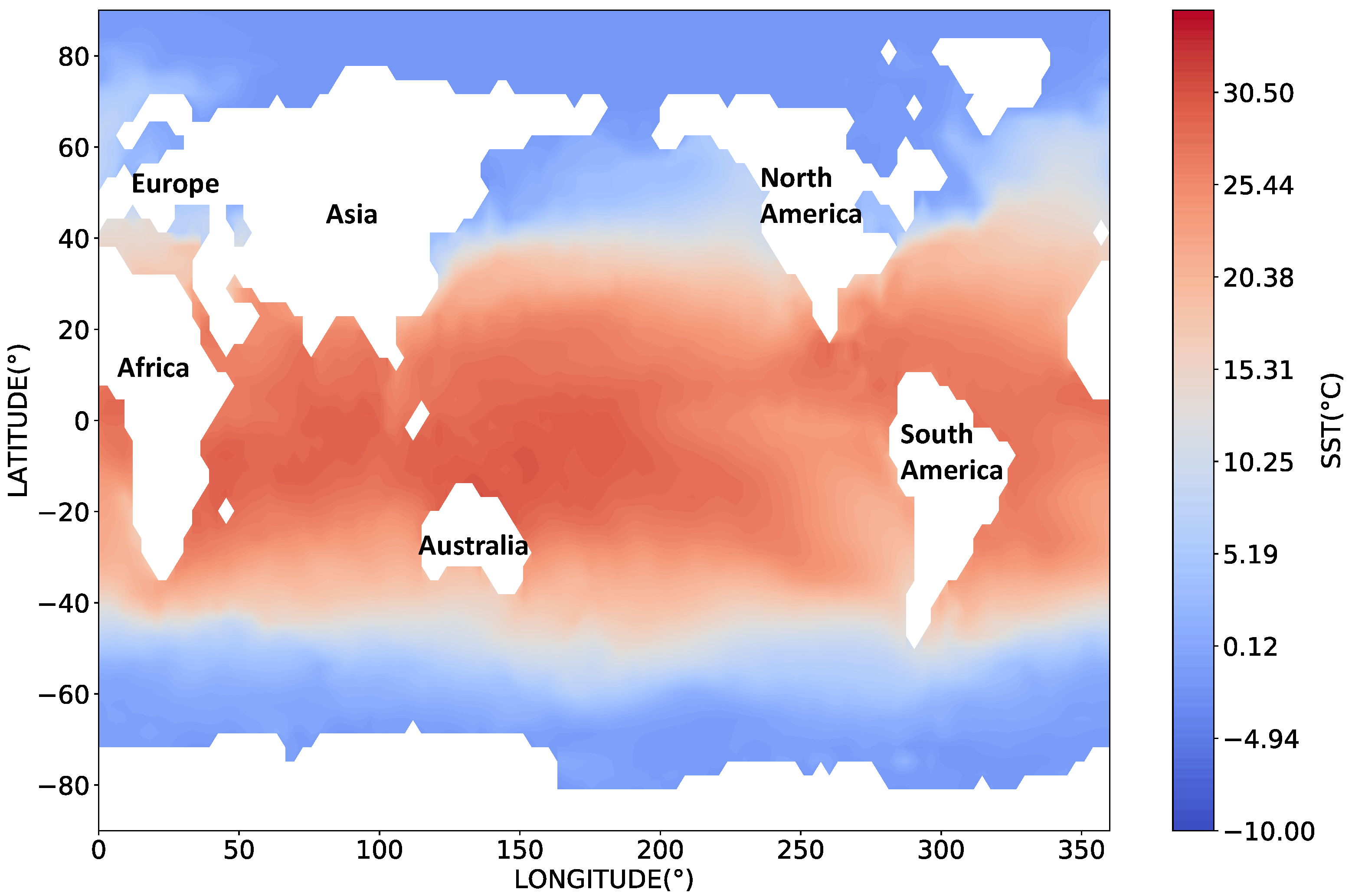
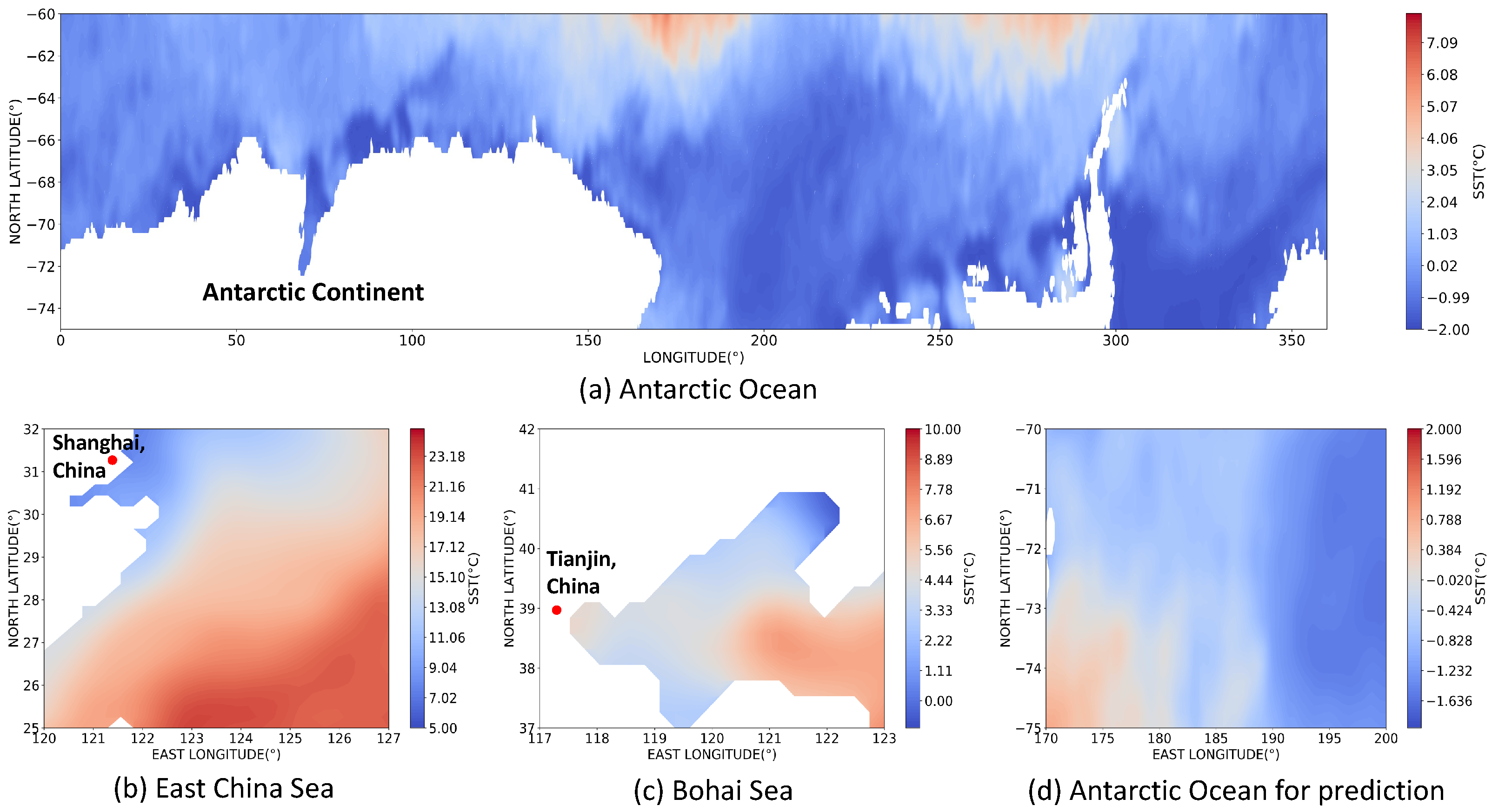
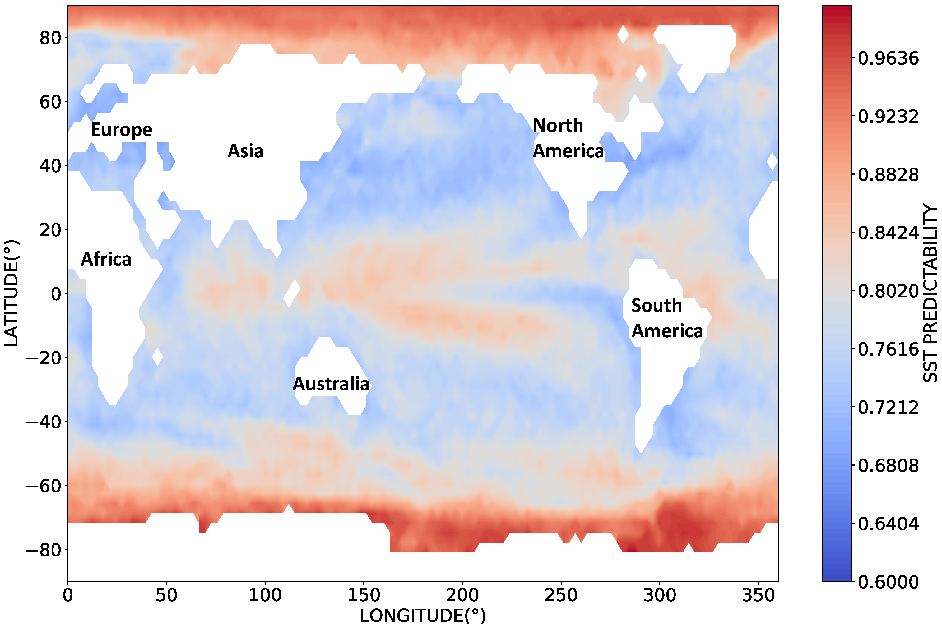
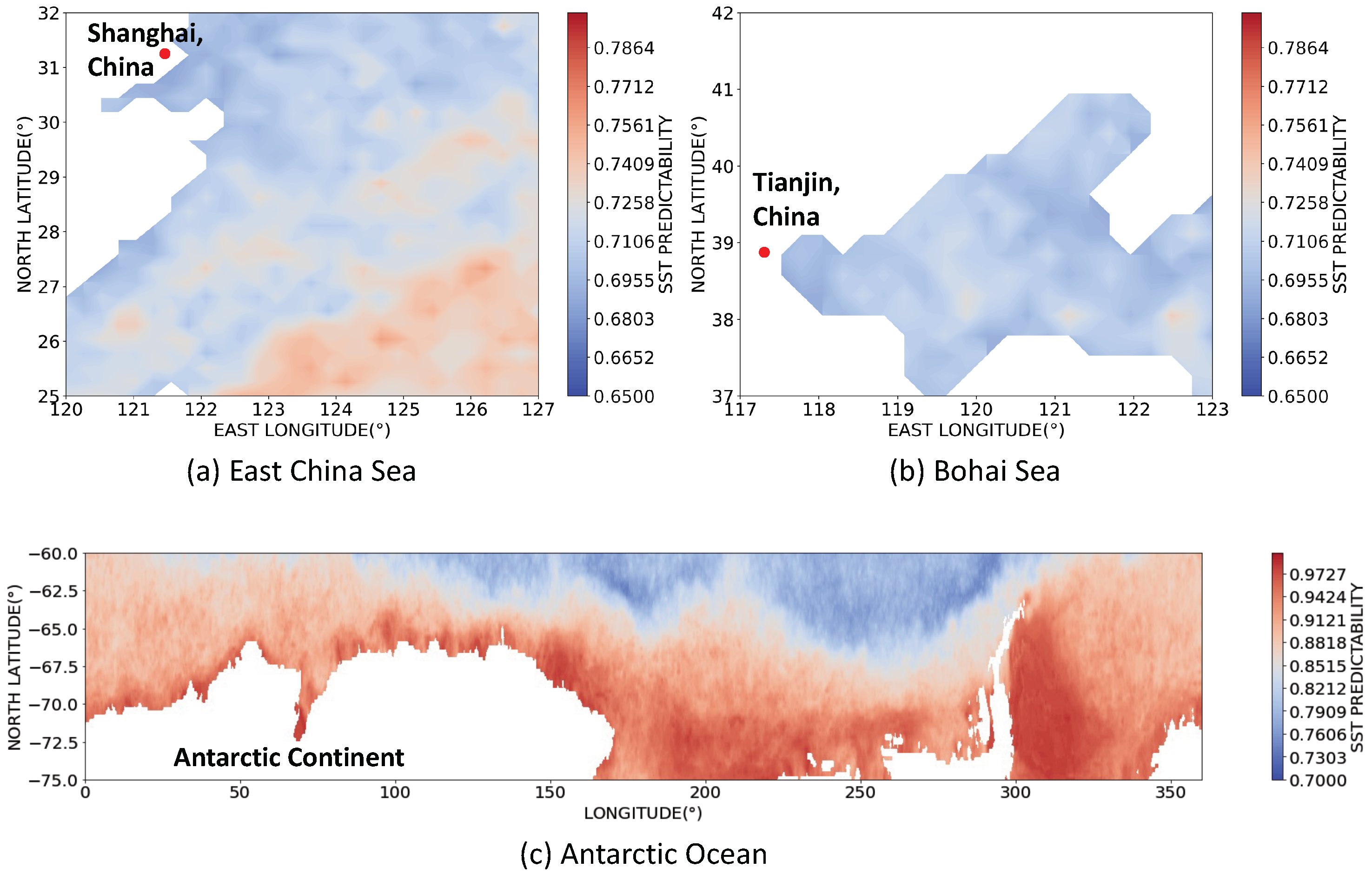
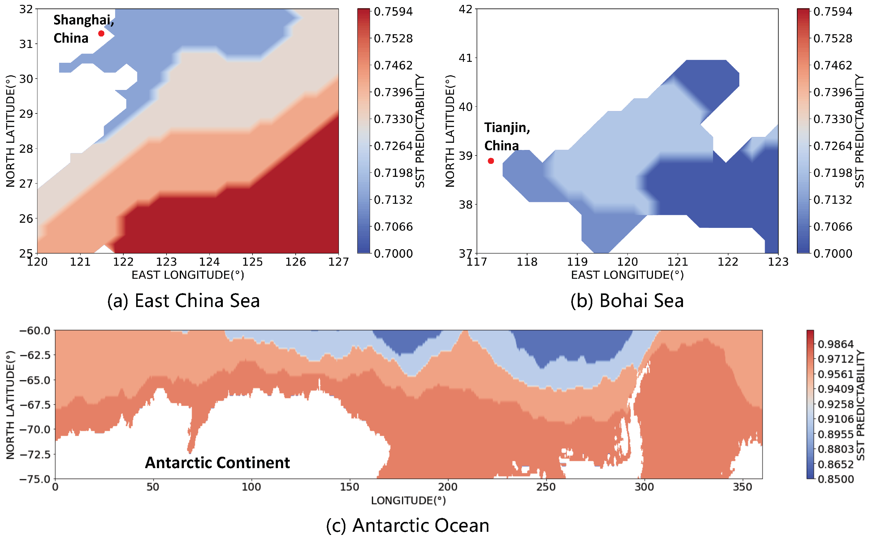
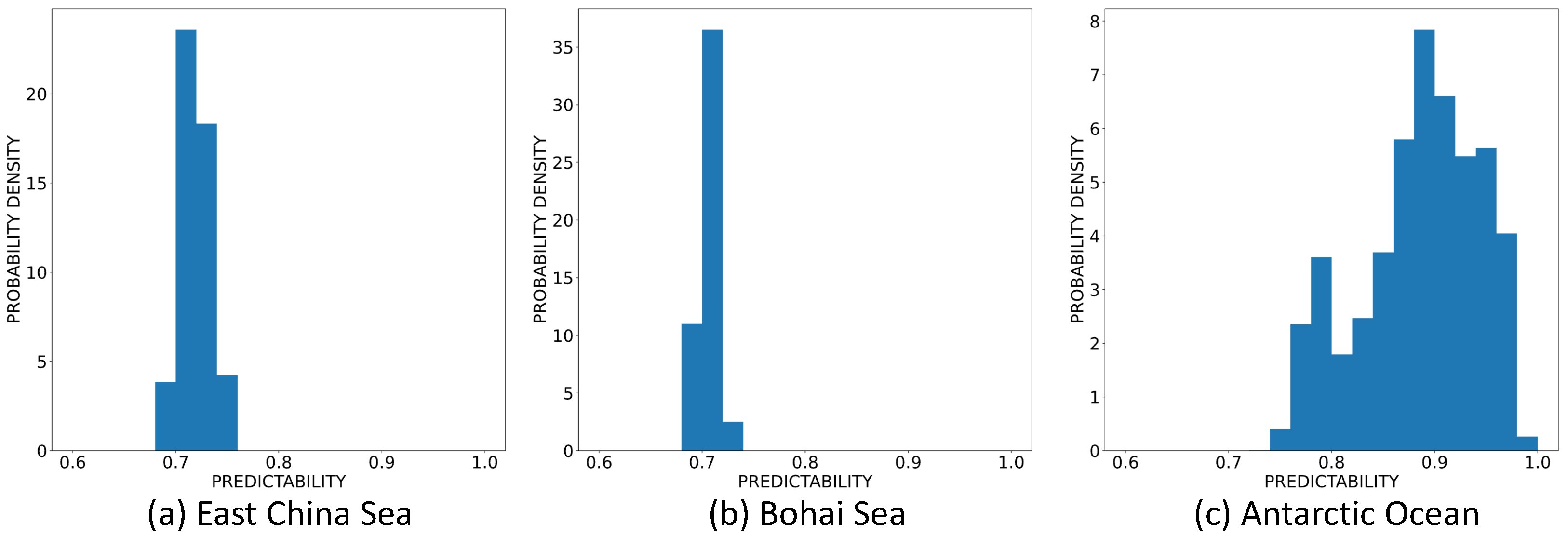
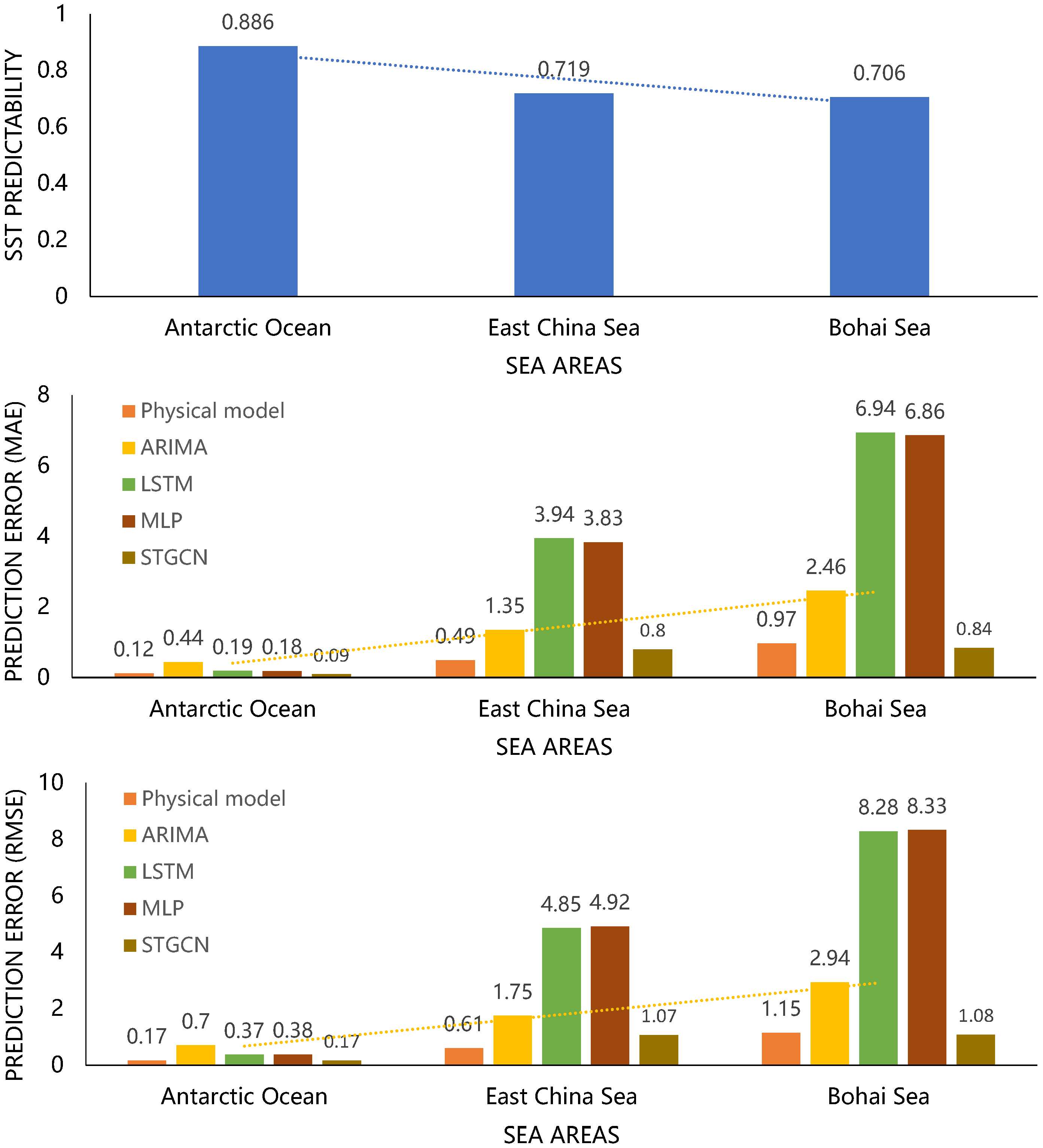
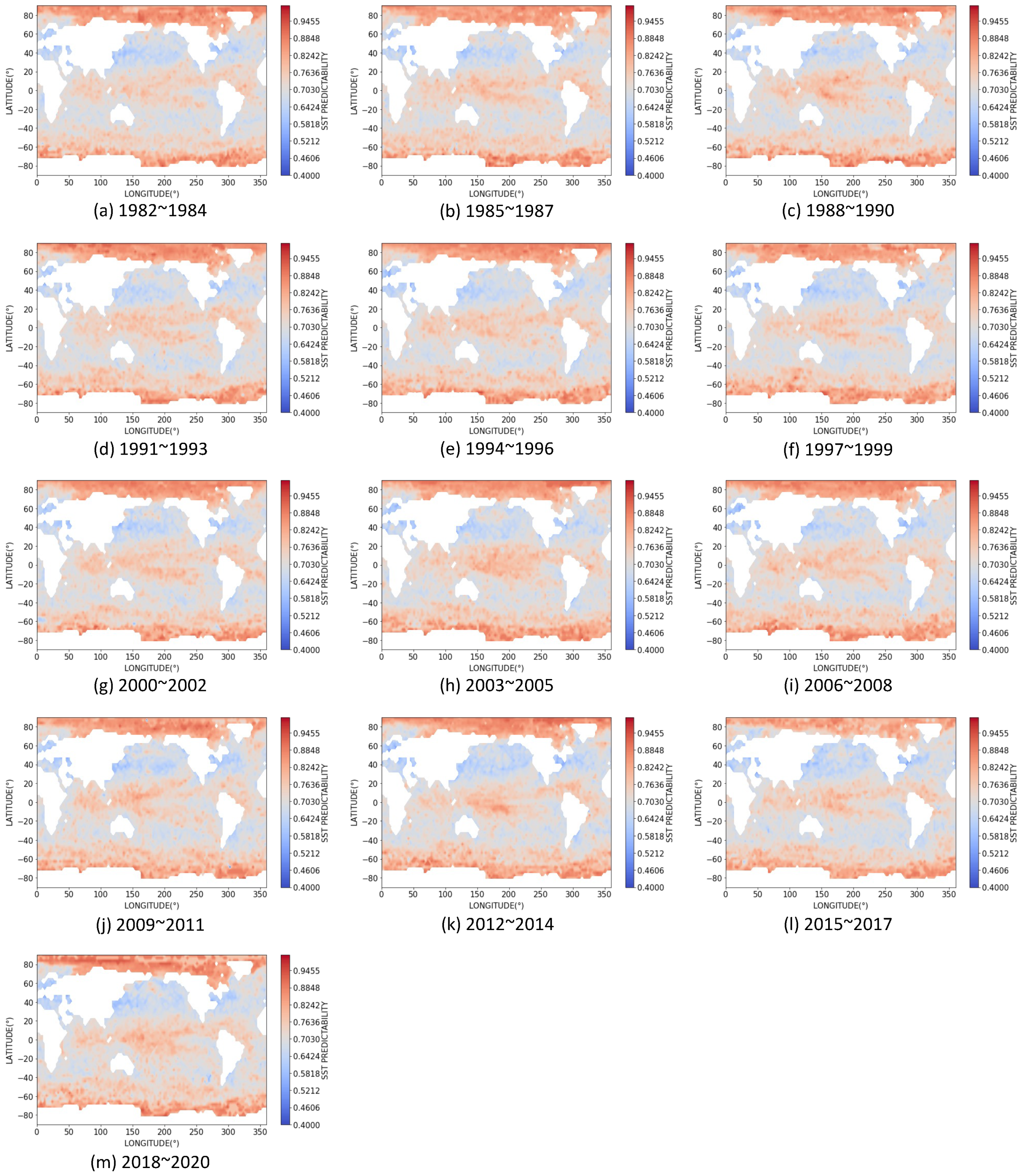
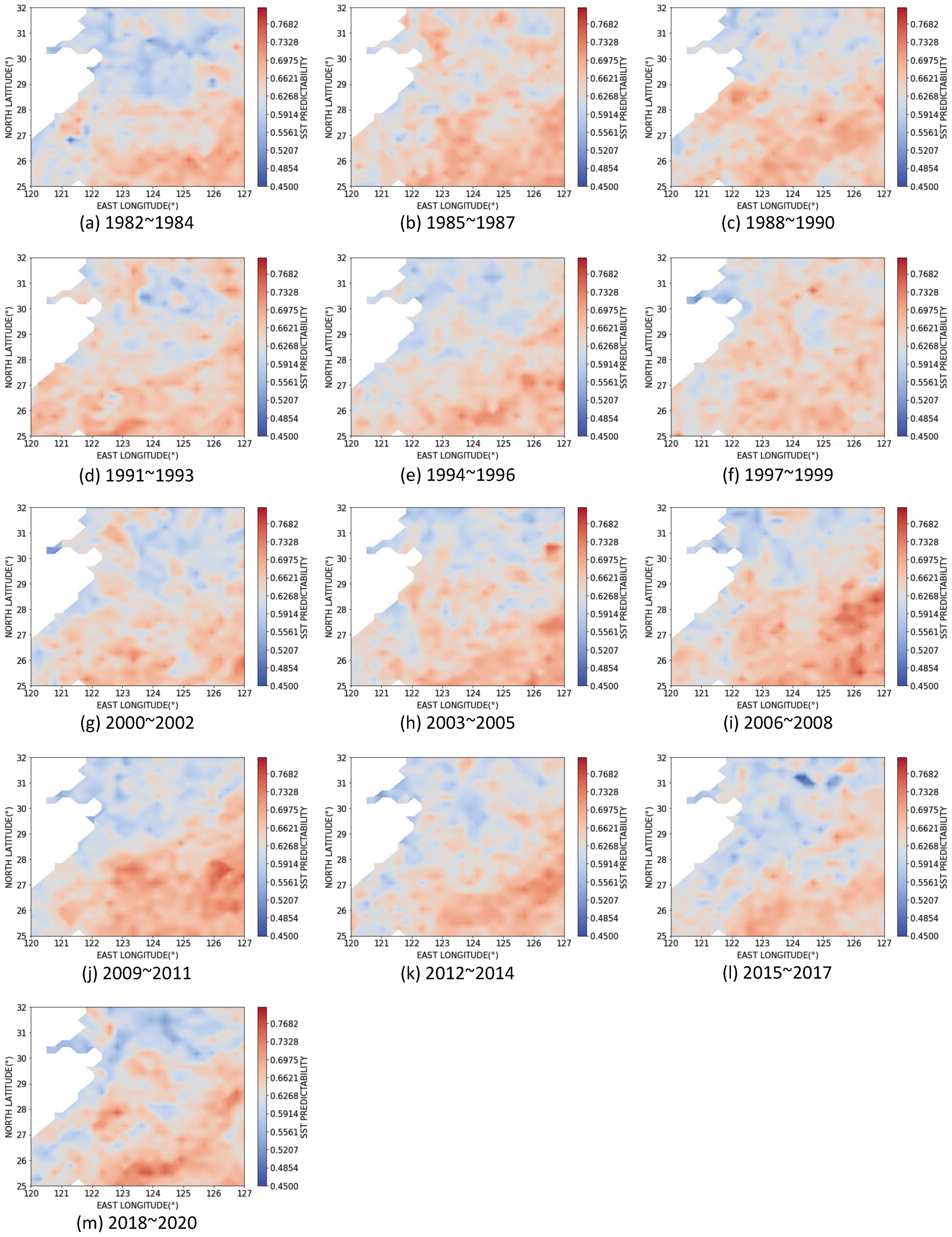
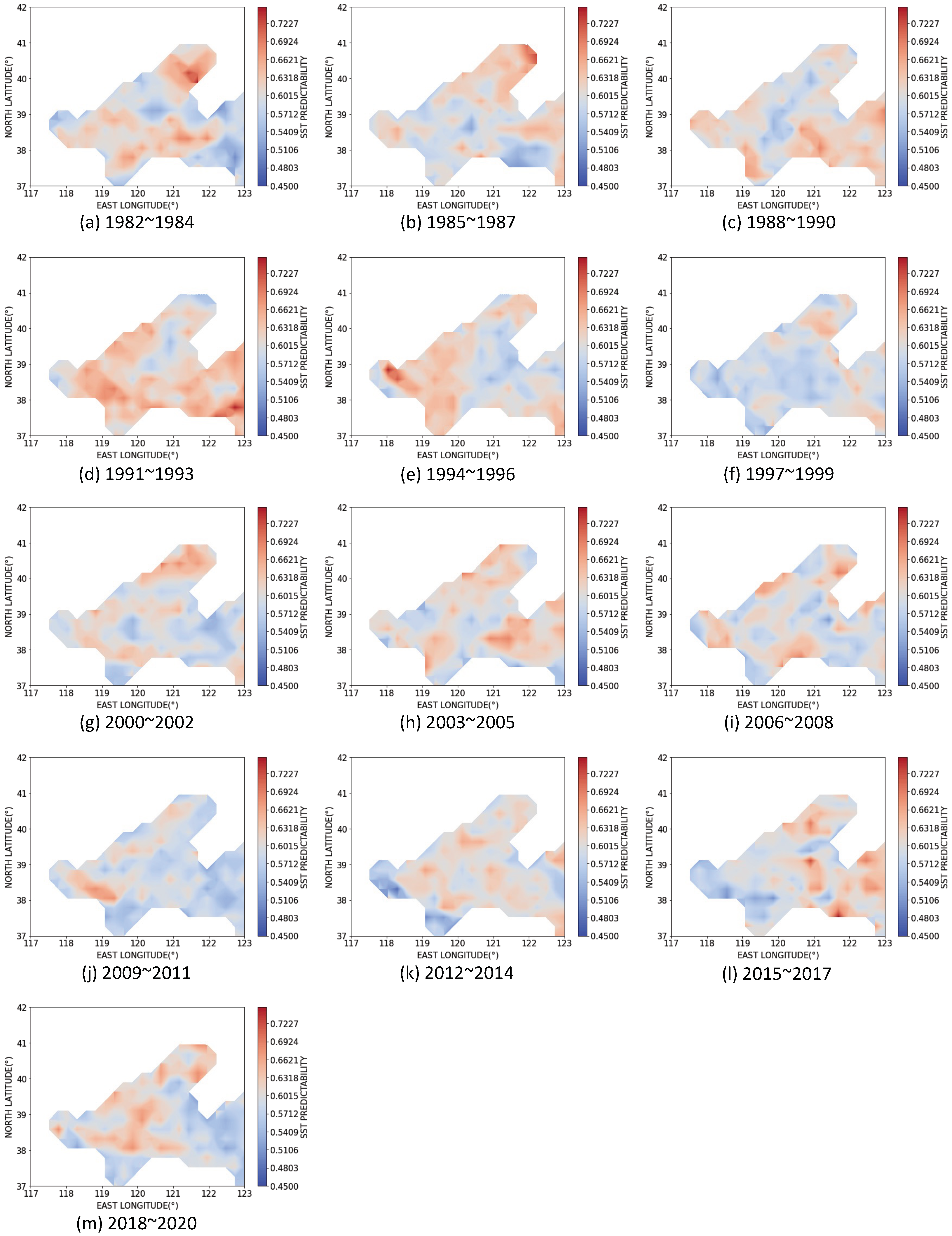
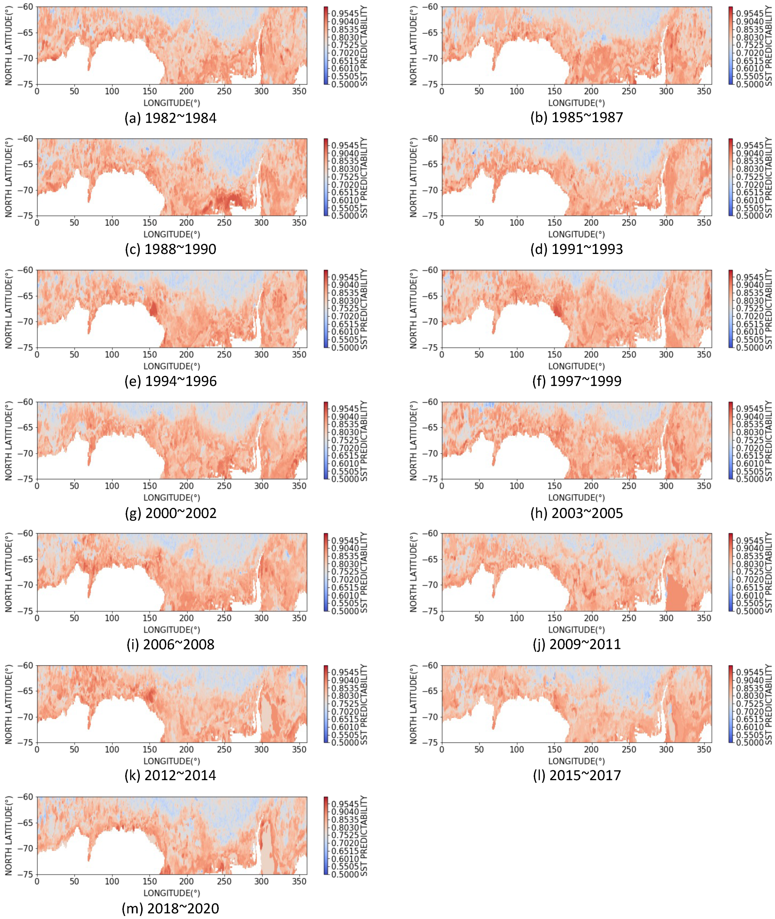
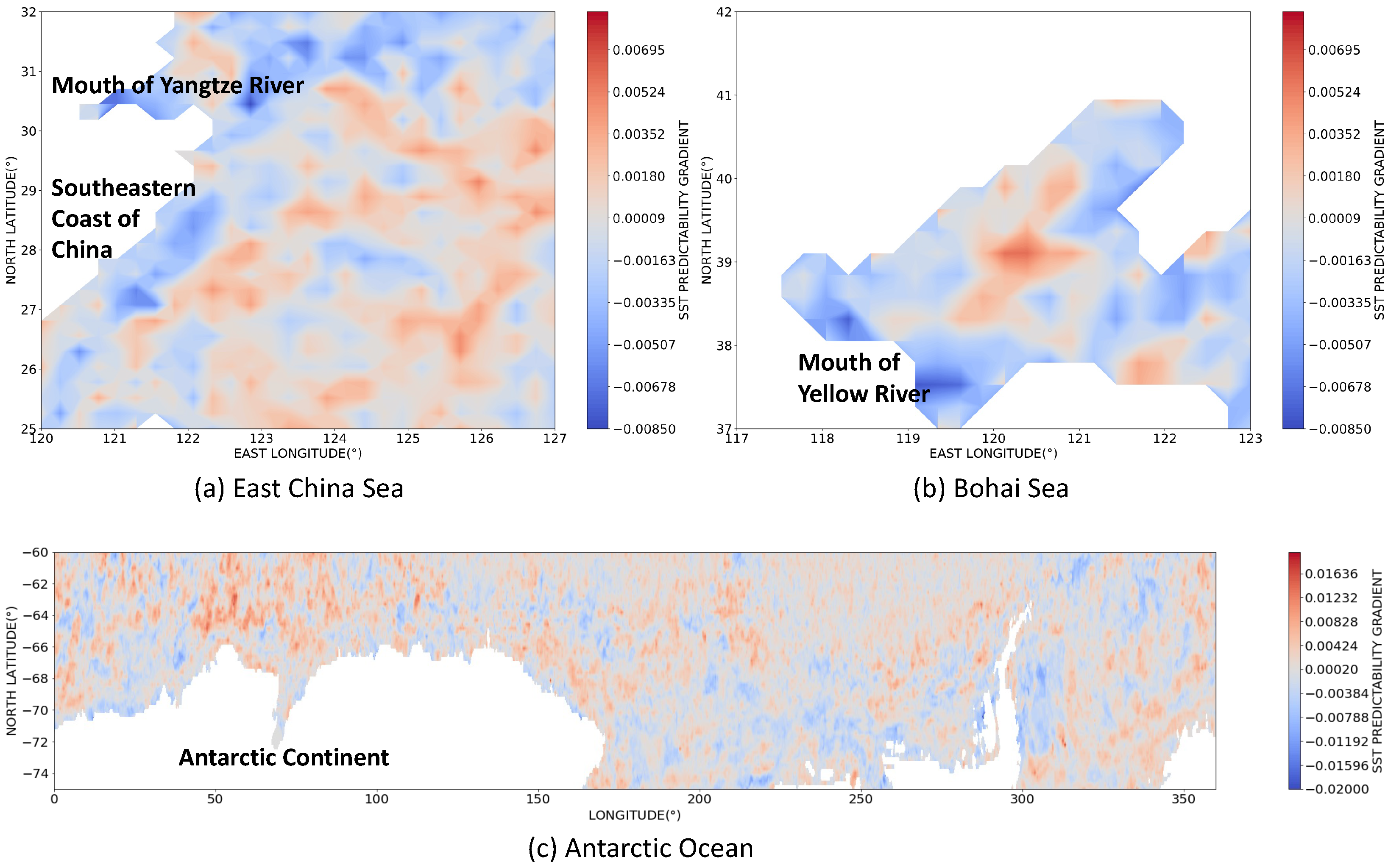
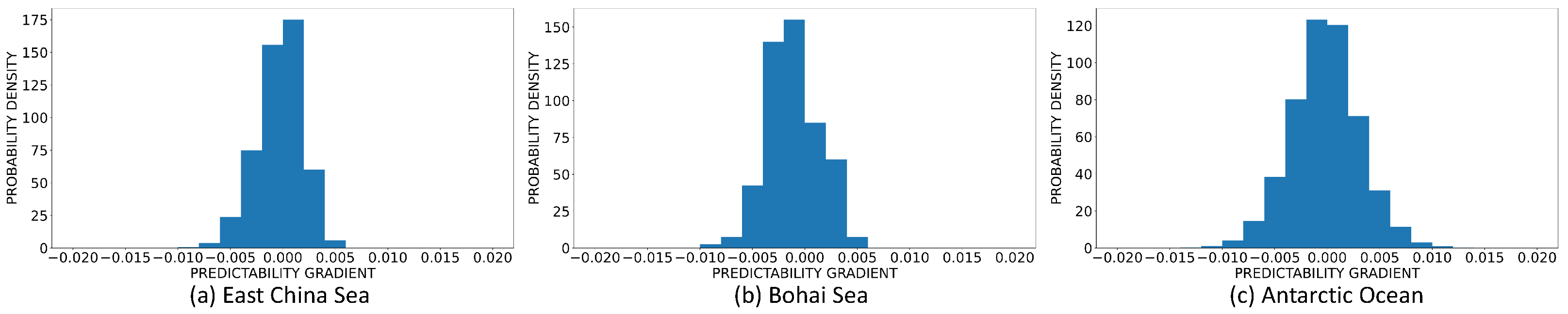
  • We introduce entropy to quantify the predictability of the coarse-grained SST in all grid sea regions of size 3 × 3 around the world, as well as the predictability of the fine-grained SST in grid regions of size 0 . 25 × 0 . 25 in three typical local sea areas (i.e., the East China Sea, the Bohai Sea, and the Antarctic Ocean), and discover the differences of SST predictability in different oceanic areas.
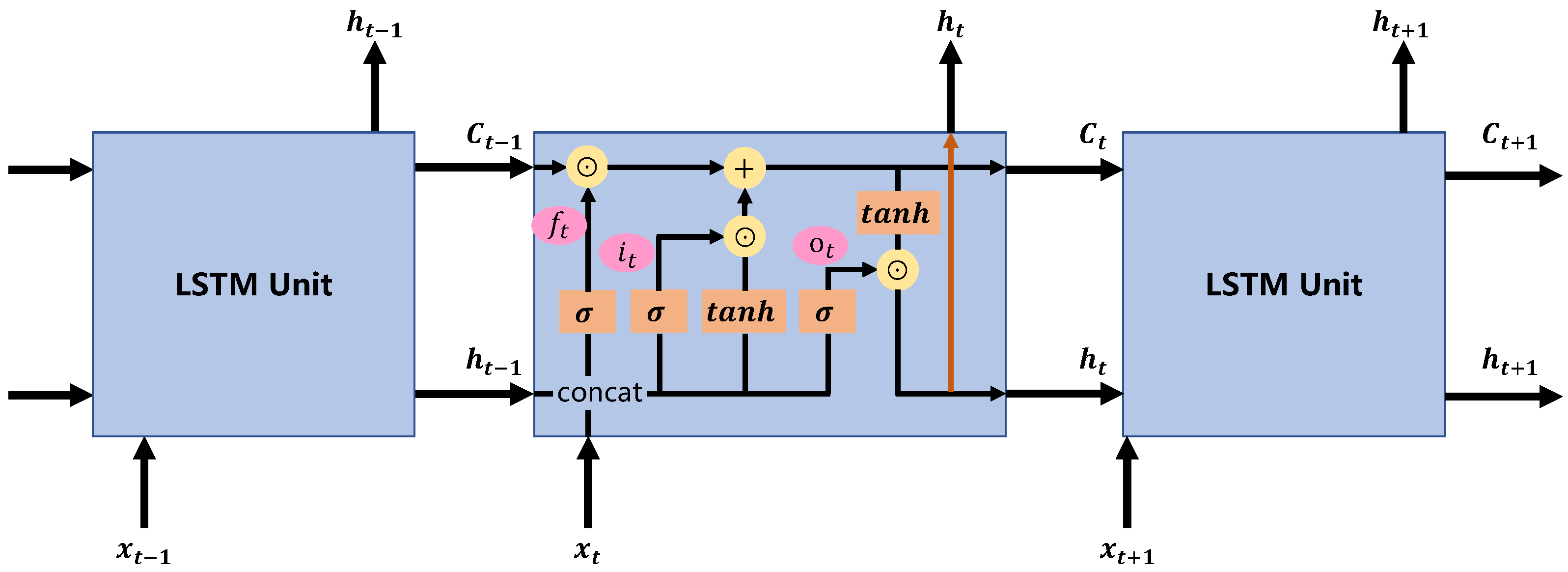
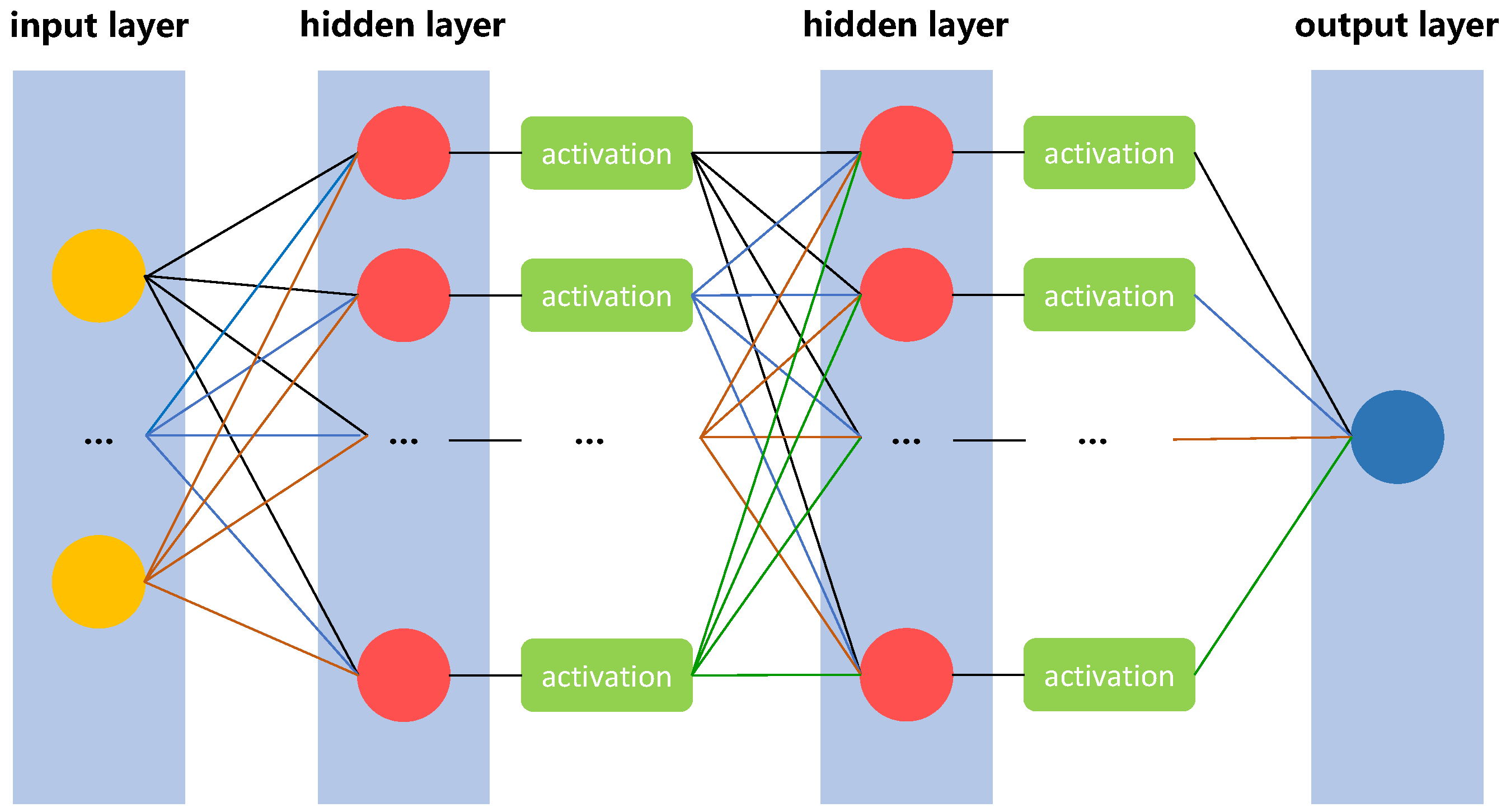
  • We develop multiple SST prediction models, including a physical model, i.e., Copernicus Marine global analysis and forecast product, AutoRegressive Integrated Moving Average(ARIMA) model, Long Short-Term Memory(LSTM) model, Multi-layer Perceptron (MLP) model, and Spatio-Temporal Graph Convolutional Network (STGCN) model, to make SST prediction. The results of these models demonstrate the effectiveness of the predictability evaluation method.
  • We analyze the dynamics of the predictability of SST over a long time period from both global and local aspects, and identify the important causes that lead to the changes in SST predictability.
For the rest of this work, we will describe the material and the proposed methods in Section 2 and present the experiment results in Section 3. Finally, Section 4 concludes the whole work.

2. Material and Methods

2.1. Datasets

In this work, we use the Optimum Interpolation SST(OISST) V2 High-Resolution dataset from National Oceanic and Atmospheric Administration (NOAA) (https://psl.noaa.gov/data/gridded/data.noaa.oisst.v2.highres.html, accessed on 5 November 2022). This dataset provides global daily SST records from 1981 to the present, and the spatial resolution is 0 . 25 × 0 . 25 . OISST V2 is based on the blending of both in situ and satellite observations. The satellite observations are provided by multi-satellite sensors, such as AVHRR and VIIRS, and the in situ ship and buoy data used is of NCEI merged TAC + Binary Universal Form for the Representation (BUFR) of meteorological data format. In general, the satellite SST biases are corrected with float SST observations such as Argo [29]. The predictability of SST should be analyzed from a large time scale since short-term SST is usually of high dynamics and uncertainty. Therefore, we calculate the monthly average SST using daily SST records to evaluate the predictability of SST.
We first quantify the predictability of the coarse-grained SST in all grid sea regions of size 3 × 3 around the world. The SST of each 3 × 3 region R is the average value of the SST records of the 12 × 12 = 144 grid regions of size 0 . 25 × 0 . 25 in R. Figure 1 shows the global monthly average SST in January 2002.
We then quantify the predictability of fine-grained SST in three local sea areas, i.e., East China Sea ( 25 N– 32 N, 120 E– 127 E), Bohai Sea ( 37 N– 42 N, 117 E– 123 E) and Antarctic Ocean ( 60 S– 75 S, 0 E– 360 E). Since the area of the Antarctic Ocean is quite large and requires too many hardware resources to train the deep learning prediction models, we further select a smaller area of ( 70 S– 75 S, 170 E– 200 E) to make SST predictions. Figure 2 illustrates the monthly average SST in January 2002 for three local sea areas, as well as the selected Antarctic Ocean area for SST prediction.
For SST predictability evaluation and SST prediction, we use the monthly average SST from 2002 to 2021. For the dynamic analysis of SST predictability, we use the monthly average SST from 1982 to 2020, to analyze the dynamic changes over a long period of time. The long time range can be divided into more fine-grained time periods, and help make more accurate dynamic analysis.

2.2. Problem Statement

We divide the sea area of interest into N = L × W grid regions, where L and W are the numbers of grid regions along the latitude and longitude, respectively. Each grid region R i is the spatial unit of SST predictability, which corresponds to an SST series x i . The SST records for all grid regions form a matrix X R N × T , where T is the number of time slots, and is also the temporal unit of the SST predictability.
Given the SST series x i for grid region R i , we aim to find a function f to measure the predictability Π i for x i , i.e.,
Π i = f ( x i )
Then, the predictability of all the grid regions can be measured as
Π = F ( X )
where F represents the algorithm that circularly uses f on each SST series, and Π R N is the predictability matrix for all N grid regions.

2.3. Methods

2.3.1. Entropy-Based Predictability Evaluation for SST

Entropy is often used to measure the degree of chaos in a system, and high entropy represents a chaotic system, which leads to low prediction accuracy. Thus, we can measure the predictability of SST sequences based on entropy theory, and the higher the entropy, the lower the predictability.
Given an SST series x, the temporal-correlated entropy S of x can be defined as below.
S = s x P ( s ) log 2 ( P ( s ) )
where s represents one specific sub-sequence in x and P ( s ) is the possibility of finding s in x [18].
Considering that the complexity of Equation (3) above is quite high, we use Lempel-Ziv estimator [5] to approximate it, i.e.,
S T ln T t l t
where T is the length of the entire SST series, l t represents the length of the shortest sub-sequence that appears after time-step t and never appears before time-step t in the entire SST series, and t represents the sum of all l t , t [ 1 , T ] . For example, given an SST series { 1 , 2 , 3 , 4 , 1 , 2 , 5 , 6 } , then l 1 means the length of the shortest sub-sequence that appears after time-step 1, i.e., the first element in the series, and never appears before time-step 1. Then l 1 equals 1, which is the length of the sub-sequence { 2 } , i.e., the shortest sub-sequence that never appears in the preceding sub-sequence { 1 } . l 2 and l 3 also equal to 1. l 4 equals 3, which is the length of the sub-sequence { 1 , 2 , 5 } after time-step 4, since { 1 } and { 1 , 2 } already appear in the preceding sub-sequence { 1 , 2 , 3 , 4 } . The entropy not only considers the frequency of different elements in the series, but also considers the temporal patterns of the series [30].
With entropy S of SST series x, according to Fano’s inequality, the maximum predictability Π m a x , i.e., the maximum probability of accurately predicting the SST with any prediction method, of x can be estimated by the following formula [18].
S = Π m a x log 2 ( Π m a x ) ( 1 Π m a x ) log 2 ( 1 Π m a x ) + ( 1 Π m a x ) log 2 ( M 1 )
where M is the number of distinct elements in the SST series x. The maximum predictability Π m a x is between 0 and 1, and the larger the value of Π m a x , the higher the probability of accurately predicting the SST. Specifically, 0 represents no accurate prediction can be made, and 1 represents that we can achieve 100% accurate prediction.
To solve Equation (5), we deform it into the following equation.
S + Π m a x log 2 ( Π m a x ) + ( 1 Π m a x ) log 2 ( 1 Π m a x ) ( 1 Π m a x ) log 2 ( M 1 ) = 0
In Equation (6), there is only Π m a x unknown. Since the equation cannot be solved directly, we adopt Newton’s method to perform constant iterations to obtain the approximation of Π m a x .
According to Equations (4) and (6), we need to frequently evaluate whether two sub-sequences are equal and count the number of distinct elements in the whole time series. When evaluating the predictability of transportation and human mobility, the sequences we use to calculate entropy and predictability are usually position sequences, and it is straightforward to compare whether two sub-sequences are equal. However, for the SST time series, the SST records are floating-point numbers, and exactly equal records rarely occur in the series. To address this issue, we set a threshold ϵ , and two SST records are considered to be the same if their difference is less than ϵ . For example, if ϵ is set to 0.2, two SST series { 1 , 1.5 , 1.7 , 2.2 } and { 1.1 , 1.3 , 1.6 , 2.3 } are equal. The value of ϵ directly influences the calculated predictability. When ϵ is set to be larger, then more floating points in the sequence are the same, the sequence is less chaotic, the calculated entropy is smaller, and therefore the larger predictability is obtained. As the value of ϵ increases, the calculated predictability increases accordingly. However, it does not affect the relative size between the predictability corresponding to different SST series. We will further analyze the correlations between ϵ and predictability via experiments in Section 3.

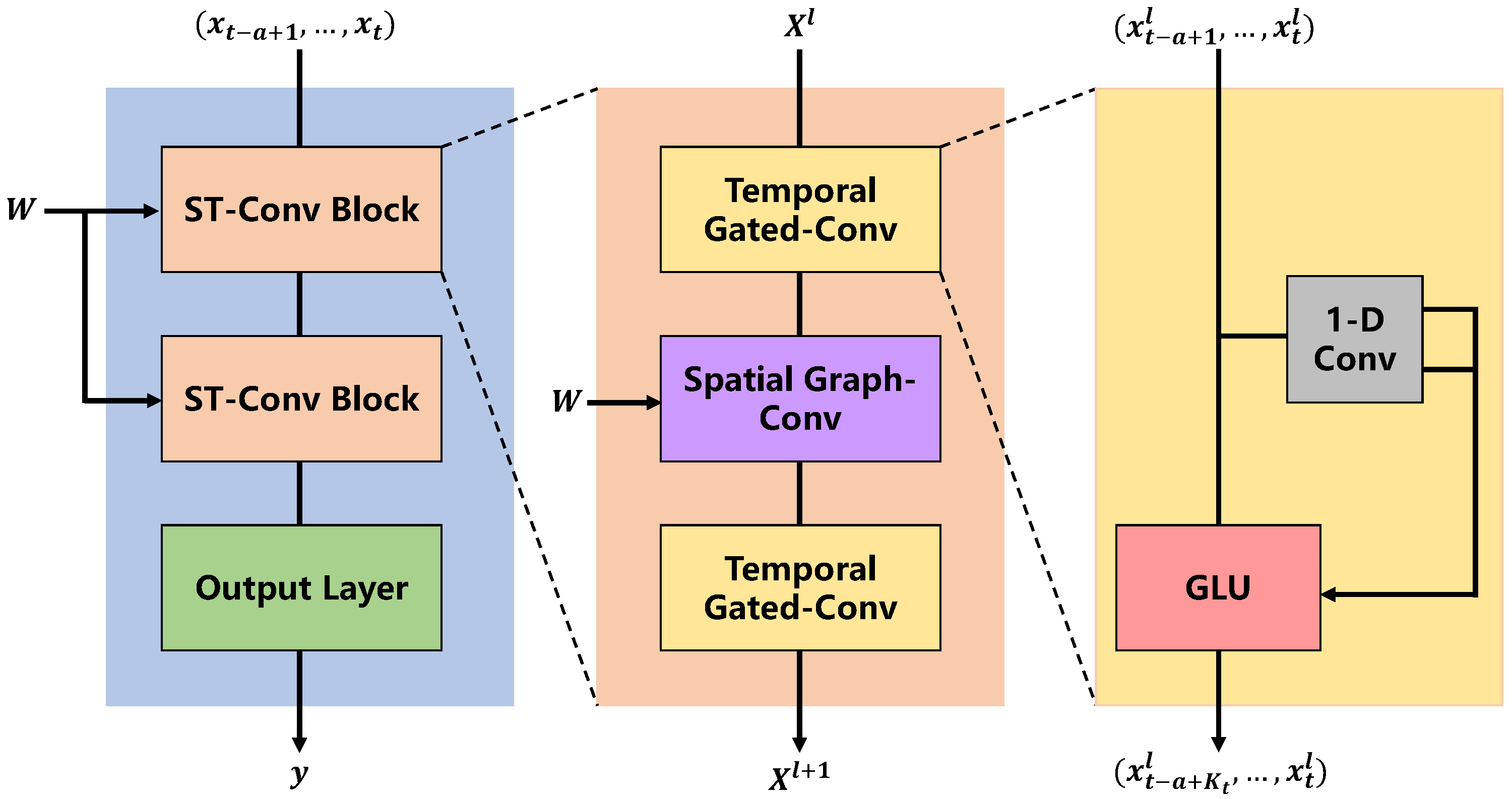
2.3.2. SST Prediction Models

For each specific time slot t, the SST records for all regions are represented by X t R N . Given the historical SST of a time slots X t a + 1 , X t a + 2 , . . . , X t , SST prediction aims to predict the SST records in next b time slots, i.e.,
X t + 1 , X t + 2 , . . . , X t + b = P ( X t a + 1 , X t a + 2 , . . . , X t )
where P is one certain SST prediction method.
In this work, five representative SST prediction models, i.e., a physical model, ARIMA, LSTM, MLP, and STGCN, are introduced to analyze the correlations between the prediction performance and SST predictability in different sea areas. The techniques of the five models are briefly discussed below.
A. Physical Model
The physical model we use is Copernicus Marine global analysis and forecast product with the product ID of GLOBAL_ANALYSISFORECAST_PHY_001_024. This product provides two kinds of data, i.e., aggregated analysis data and 10 days of global ocean forecasts data, and the resolution of the data in the model is 1 / 12 × 1 / 12 . The variables of the model include potential temperature, salinity, and currents information on a 3D scale, i.e., including data of different depths, sea surface level, bottom potential temperature, mixed layer thickness, sea ice thickness, sea ice fraction, and sea ice velocities information on a 2D scale in global ocean area. The product contains 16 different datasets of different ocean variables, and we use the dataset cmems_mod_glo_phy-thetao_anfc_0.083deg_P1M-m, which contains monthly average potential SST for our SST prediction experiment.
B. ARIMA
The autoregressive integrated moving average (ARIMA) model is a time series analysis method, which includes three modules, i.e., autoregression (AR), integrated (I), and moving average (MA). AR module considers the relationship between the value at the current time slot and the values at several previous time slots. I module converts the original data into differential data to eliminate the influence of non-stationary information, such as trend, in time series. MA module considers the relationship between the value at the current time slot and the errors at several previous time slots. ARIMA model works as follows:
A R I M A ( p , d , q ) = A R ( p ) + I ( d ) + M A ( q )
where A R ( p ) is the autoregressive module, I ( d ) is the integrated module, and M A ( q ) is the moving average module. The lag order p indicates the number of historical time slots we consider in A R module, and d represents the degree of differencing, which indicates the number of times that the time series are differenced, and q is the order of moving average, which indicates the number of historical time slots we consider in M A module.
To determine the value of model parameters ( p , q ) , we first set the maximum values and minimum values for ( p , q ) , i.e., ( p m a x , q m a x ) and ( p m i n , q m i n ) , and then calculate the AIC value of ARIMA model corresponding to each ( p , q ) combination within the range. Finally, we select the model with the minimum AIC value to perform prediction. The full name of AIC is Akaike Information Criterion, which is a measure of the fitting performance of a statistical model, and the smaller the value of AIC, the better the fitting performance of the model. In the general case, the AIC can be described as:
A I C = 2 k 2 ln L
where k represents the number of model parameters and L is the likelihood function value.
C. LSTM
Long Short-Term Memory(LSTM) model [31] is a typical Recurrent Neural Network (RNN) model that can capture the long-term dependency in time series, and address the issues of gradient explosion and gradient disappearance in RNN. Figure 3 illustrates the structure of LSTM which consists of forget gate unit, input gate unit, and output gate unit.
The meaning of the symbols in Figure 3 is explained in the figure caption. The operations of LSTM can be summarized below.
f t = σ ( W f · [ h t 1 , x t ] + b f ) i t = σ ( W i · [ h t 1 , x t ] + b i ) c t = t a n h ( W C · [ h t 1 , x t ] + b C ) C t = f t C t 1 + i t c t o t = σ ( W o · [ h t 1 , x t ] + b o ) h t = o t t a n h ( C t )
where W f , b f , W i , b i , W C , b C , W o , b o are the parameters to be learned during the training process. σ , t a n h , f t , i t , o t , ⊙, +, x t , h t 1 , C t all have the same meanings with the symbols described in the caption of Figure 3. c t is an intermediate variable to help calculate C t at time-step t, [ , ] is the operation of concatenating the matrices x t and h t 1 , and · is the operation of matrix multiplication.
D. MLP
Multi-layer Perceptron(MLP) [32] is one basic neural network, which contains multiple hidden layers between the input layer and output layer. Each layer in an MLP model is fully connected to the layers next to it, i.e., each neuron in each layer has a connection to each neuron in the next layer. MLP uses activation functions to make the linear transformation of each layer of the network nonlinear, therefore it could approximate any nonlinear function to learn nonlinear correlations. Figure 4 shows the structure of MLP we use for SST prediction. The activation function used in this MLP model is ReLU, i.e.,
R e L U ( x ) = m a x ( 0 , x )
where m a x ( ) function outputs the maximum value of the input data.
E. STGCN
Spatio-Temporal Graph Convolution Network (STGCN) [33] is an advanced prediction method that can learn the spatial and temporal dependencies in SST. Figure 5 illustrates the architecture of STGCN.
For SST prediction, STGCN first builds the spatial graph G = ( V , E , W ) , where V is a set of vertices, each grid region is regarded as a vertex, and all the N grid regions correspond to N vertices in the graph; E is a set of edges, representing the connections between the vertices; W R N × N denotes the weighted adjacency matrix of the spatial graph G, and it is used to conduct spatial graph convolution. In this work, the adjacency matrix W is computed based on the distances among the grids, and each element w i j in W is calculated by the formula below.
w i j = e x p ( d i j 2 δ 2 ) , i j a n d e x p ( d i j 2 δ 2 ) η 0 , o t h e r w i s e
where w i j is the adjacency weight of the edge between grid regions i and j, d i j is the distance between grid regions i and j, and parameters δ and η are used to control the distribution and sparsity of W.
As shown in Figure 5, historical SST records and the adjacency matrix W are input into the model. The Temporal Gated-Conv block learns the temporal patterns in SST records, and the Spatial Graph-Conv block learns the spatial dependencies between grid regions with the help of W. The predicted SST values are generated by a full-connection layer.

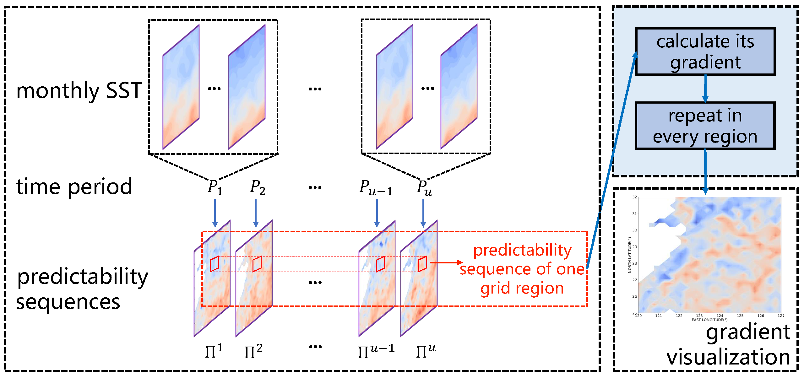
2.3.3. Analyzing the Dynamics of SST Predictability

To analyze the dynamics of the predictability of SST, we divide T time slots into u periods P 1 , P 2 , ⋯, P u , and each period has τ time slots. Then, all historical SST records are divided into u sub-matrices X 1 , X 2 , . . . , X u , where X i R N × τ . By measuring the predictability Π i R N for each SST sub-matrix X i , we can obtain a sequence of u predictability values, i.e., Π 1 , Π 2 , . . . , Π u for each grid region. Then we analyze the dynamics of the predictability of SST based on this sequence. Figure 6 presents the process for analyzing the dynamics of SST predictability.
With the predictability sequence Π 1 , Π 2 , . . . , Π u , we compute its gradient k to analyze the rising or falling trend of the predictability of SST in the corresponding grid region. First, the coordinate points ( 1 , Π 1 ) , ( 2 , Π 2 ) , . . . , ( u , Π u ) are used to represent the predictability of each time period, and they form a series of points in the two-dimensional coordinate system. Then, we calculate the gradient k of the line that can fit these coordinate points using the method of least squares, i.e.,
k = i = 1 u i Π i u i ¯ Π ¯ i = 1 u i 2 u i ¯ 2
where u is the number of time periods; i is the x-coordinate of the ith coordinate point, which is the number between 1 and u; i ¯ is the average value of all i; and Π ¯ is the average value of all Π i .
For example, the SST predictability sequence of a specific sea region in ( 57 S– 60 S, 60 E– 63 E) is shown in Figure 7. The coordinates of the points in the figure represent the predictability value of each time period. The red line is calculated using Equation (13) to fit these coordinate points. The gradient of the line, i.e., 0.00162, can be used to evaluate the dynamics of SST predictability. If the gradient is steep, it means that the speed of the predictability change in this region is fast, i.e., the SST is becoming more and more chaotic or stable. For example, the increase in human activities will lead to an increased chaotic degree of the SST in the sea areas close to land, therefore resulting in a steep decrease gradient of SST predictability.

2.4. Evaluation Settings

When calculating the predictability from entropy, we set the threshold ϵ for judging the similarity between two sub-sequences to 0.2. The maximum number of iterations in Newton’s method is set to 300.
The parameter a represents the number of time slots in historical SST records, and b is the number of time slots of SST we predict in the future, and they are set to 7 and 1, respectively, i.e., using the previous seven monthly average SST records to predict the SST in next month. When performing SST prediction with the ARIMA model, we set the model parameter ( p m a x , q m a x ) to ( 7 , 7 ) , and ( p m i n , q m i n ) to ( 0 , 0 ) . When performing SST prediction with deep learning models, we split each dataset for SST prediction into three subsets for training, validating, and testing, respectively, with a ratio of 3:1:1. During the training of deep learning models, the hyper-parameter batch size is set to 16 and the number of epochs is set to 100. Mean absolute error(MAE) and root mean square error(RMSE) are used as metrics to measure the performance of prediction models, and MAE is also used for measuring the loss in training. The MAE loss and RMSE loss are calculated as below:
M A E = 1 n i = 1 n | h ( x i ) y i | R M S E = 1 n i = 1 n ( h ( x i ) y i ) 2
where n is the number of data samples, h ( x i ) represents the prediction results using sample x i and prediction algorithm h, and y i is the true value corresponding to x i .

3. Results and Discussion

3.1. Predictability of SST

Figure 8 shows the predictability of global monthly SST from 2002 to 2021, where the dark red color indicates high predictability while the dark blue color indicates low predictability. The predictability near the land is generally lower than the predictability away from the land. This may be because land-to-ocean heat exchange at depth of 10 microns influences the SST predictability. Another reason may be that the various human activities around the land have complex impacts on SST, such as shipping and aquaculture, which makes the SST more chaotic and less predictable. The predictability of SST near the equator is high due to the fixed currents, i.e., North Equatorial Current, South Equatorial Current, and Equatorial Counter Current. In addition, there are no significant seasonal changes near the equator and the solar radiation and temperatures are relatively stable. Therefore, the SST variation will also be relatively stable due to the sea-air heat exchange and sunlight, making the SST predictability near the equator higher. The SST predictability values in both poles are also really high and close to 1. The possible reason is that the SST records at the poles are low and stable all year around, and there is little human interference, making the SST variation there very regular.
Figure 9 illustrates the predictability of SST in the East China Sea, the Bohai Sea, and the Antarctic Ocean from 2002 to 2021. In the East China Sea, the SST predictability near the mouth of the Yangtze River and the southeastern coast of China is much lower than that far away from the mainland. The reason may be that the heat fluxes from land to ocean, the water flow from the mouth of the Yangtze River into the ocean, and the high level of human activities such as shipping, tourism, and fishing around the land all have large impacts on SST, making the SST less predictable in these areas. In the Bohai Sea, the SST predictability near the land is also lower than that in the center of the sea. The predictability of SST in the Bohai Sea is generally lower than in the East China Sea since the Bohai Sea is an enclosed inland sea with shallower water, which is more easily affected by heat fluxes and human activities.
For the Antarctic Ocean, the SST predictability close to the Antarctic continent is very high, which is different from other sea areas. This is because the Antarctic continent is glacial and has few human activities, and the temperature there is low and stable all year round. The SST predictability in the Antarctic Ocean is much higher than that in the East China Sea and the Bohai Sea, which indicates that the SST in the Antarctic Ocean is the most regular of the three areas.
We also use a clustering algorithm, K-means, to cluster the original SST sequences, and automatically cluster the sea area into different regions. We obtain the SST sequence for each region by averaging the data points of 0 . 25 × 0 . 25 resolution within that region in the OISST V2 dataset, and then use the SST sequence of each region to perform the predictability evaluation experiment. K-means is a common clustering algorithm and can be written as
C = K m e a n s ( X , k )
where X is the input data and k is the number of clustering classes. For better clustering, we use different k values to perform the clustering experiment, and then use the Calinski–Harabaz Index to determine the selection of k with the best clustering effect. We choose the k with the highest Calinski–Harabaz Index result as the parameter for the final clustering experiment.
We conducted experiments on the three local sea areas, and the Calinski–Harabaz Index peaked at k = 4 on all SST data of the three sea areas. Figure 10 shows the predictability results in the East China Sea, the Bohai Sea, and the Antarctic Ocean with clustered SST data.
We can see from Figure 10 that the predictability of SST shows regional characteristics, and its spatial distribution characteristics are consistent with Figure 9.
Figure 11 presents the probability density distributions of the SST predictability in the three sea areas. The SST predictability values of most grid regions in the East China Sea are higher than 0.7, and the SST predictability values in the Bohai Sea are concentrated at 0.7. The SST predictability values in the Antarctic Ocean are above 0.7, and most grid regions have SST predictability values larger than 0.9. The probability density distribution of the predictability of SST in the Antarctic Ocean appears to be more disordered than the other two sea areas. This is because the area of the Antarctic Ocean is quite large, and covers very high SST predictability values around the Antarctic continent and low SST predictability near the South Pacific Ocean.
According to Figure 9, Figure 10 and Figure 11, the relationship of the SST predictability among the three sea areas is
Π A n t a r c t i c > Π E C S > Π B o h a i
Figure 12 shows the relationship between the threshold ϵ and the average SST predictability of global sea area. With the increase of ϵ , the SST predictability increases accordingly because the SST sequences become less chaotic, and more sub-sequences are regarded as the same. We set the value of ϵ to 0.2 because the average predictability it corresponds to, i.e., 0.808, is a reasonable middle value among the values listed in the figure. If the value of ϵ is set too large, the SST predictability will be too high, and more different SST sequences are approximated as the same sequences, resulting in a less clear distinction between the SST predictability of different sea regions.

3.2. SST Predictability vs. Prediction Performance

Figure 13 illustrates the average SST predictability and prediction error (i.e., MAE and RMSE) of five prediction models in three sea areas. All five prediction models perform the worst in the Bohai Sea and perform the best in the Antarctic Ocean, which conforms to the predictability of SST in the three sea areas. The results in Figure 13 indicate that high predictability usually corresponds to low prediction error, which proves the effectiveness of the predictability evaluation method. The prediction loss of STGCN is much less than LSTM and MLP since it can effectively learn spatial and temporal dependencies in SST. The physical model is Copernicus Marine global analysis and forecast product GLOBAL_ANALYSISFORECAST_PHY_001_024, and we use the aggregated analysis data in the product instead of raw prediction data, which produces quite good prediction results.

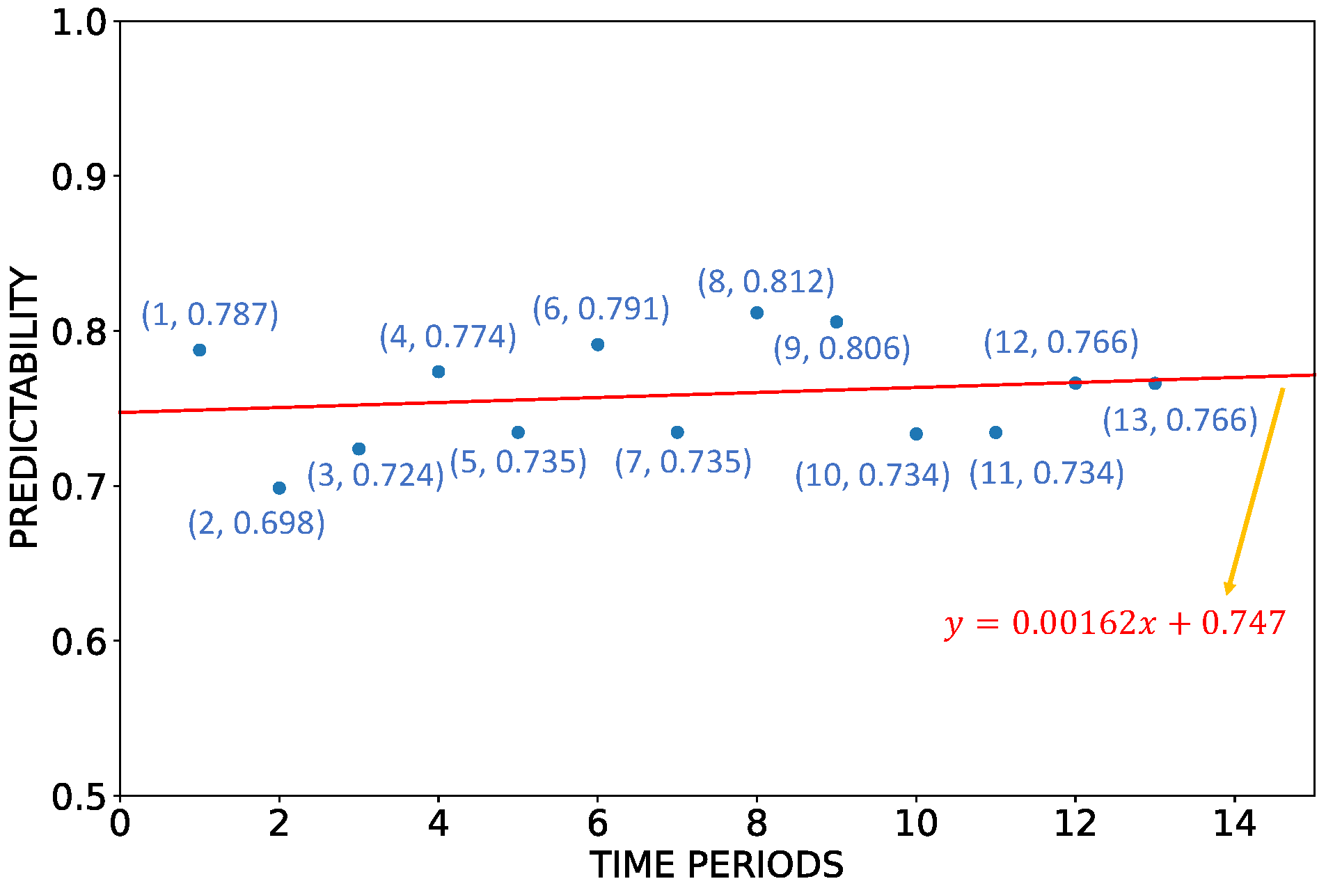
3.3. Dynamics of SST Predictability

We further analyze the dynamic changes in SST predictability over time. To this end, we divide the time range from 1982 to 2020, i.e., 39 years, into 13 small time periods, each covering 3 years, and calculate the predictability of SST in each period. Figure 14 visualizes the predictability of SST around the world in 13 time periods. Compared to the 20-year global SST predictability, the periodic results still show high predictability around the two polar areas and in the equatorial ocean current regions.
Figure 15, Figure 16 and Figure 17 show the predictability of SST in 13 time periods in the East China Sea, the Bohai Sea, and the Antarctic Ocean, respectively. According to Figure 15, the color near the mouth of the Yangtze River becomes bluer, which means the predictability becomes lower. The reason may be that the increasing human activities, such as shipping in the mouth of the Yangtze River, have increasing impacts on SST. According to Figure 16, the SST predictability in the whole Bohai Sea area varies dramatically over time. This is because the average depth of the Bohai Sea is very shallow and the SST there is not stable. In addition, the Bohai Sea is an inland sea with many human activities, making its SST very easily affected by various external factors. Figure 17 shows that most regions in the Antarctic Ocean have consistently high predictability because there is little interference to the SST in Antarctica.
To explore the dynamic change trends of SST predictability, we measure the gradient of the predictability sequences in three local sea areas. Figure 18 shows the gradient of the SST predictability sequences in the East China Sea, the Bohai Sea, and the Antarctic Ocean. The predictability of SST in the regions close to the mouth of the Yangtze River, the mouth of the Yellow River, and the southeastern coast of China decrease rapidly, which means the SST records of these regions become more and more chaotic. This may be due to China’s rapid economic development in recent decades and the increased shipping and industrial use of the mouths of the two major rivers and the ports along the coast. The SST predictability in the Antarctic Ocean shows more drastic changes than in the East China Sea and the Bohai Sea. Although the overall predictability of the Antarctic Ocean is consistently high, the gradient values of predictability are different from region to region, and the absolute values of the gradients are greater than the East China Sea and the Bohai Sea. This may be due to global warming and melting glaciers, which have a greater impact on the climate of Antarctica, resulting in abnormal SST.
Figure 19 shows the probability density of the predictability gradient of the East China Sea, the Bohai Sea, and the Antarctic Ocean. The Antarctic Ocean has more regions with sharp changes in gradient than the East China Sea and the Bohai Sea. The maximum and minimum gradients in the three sea areas are shown in Table 1, and the Antarctic Ocean has the most extreme predictability variations. The reason for the drastic changes in the SST predictability in the Antarctic Ocean could be the melting of glaciers caused by global warming.

4. Conclusions

In this work, we first introduced entropy to measure the predictability of SST sequences from both global coarse-grained and local fine-grained aspects. According to the results, the SST predictability near the land is usually low, while the SST predictability away from the land is high because the SST near the land is often affected by the heat fluxes from land and human activities. Meanwhile, the SST predictability near the equator is relatively high due to the ocean currents and stable temperature and sunlight, while the SST predictability values at both poles are high since they have few human activities and the temperature there is low and stable all year round. The average SST predictability values of the East China Sea, Bohai Sea, and Antarctic Ocean are 0.719, 0.706, and 0.886, respectively. Then, we developed five prediction models, i.e., Copernicus Marine global analysis and forecast product, ARIMA, LSTM, MLP, and STGCN, to make predictions for SST sequences in the East China Sea, the Bohai Sea, and the Antarctic Ocean, and the prediction results of different sea areas are consistent with the average SST predictability in these areas, therefore proving the effectiveness of the predictability evaluation method. Finally, we divided the 39 years from 1982 to 2020 into 13 time periods, computed the predictability of SST in each period, and calculated the gradient of the predictability sequence in each region to capture the dynamic changes in SST predictability. According to the dynamic analysis, the predictability of the Antarctic Ocean changes more dramatically over time than both the East China Sea and the Bohai Sea, which may be caused by global warming and glacier melting. The results of the spatial distribution of SST predictability and its dynamic trends indicate that global warming, ocean currents, and human activities all have significant impacts on the predictability of SST. However, there are still some limitations in our work. We use reanalysis SST data from the OISST dataset, which contains SST data at different depths obtained by various collection methods such as satellites, ships, and buoys, and the SST variation at different depths will have different correlation factors. Therefore, it is difficult to identify the physical factors responsible for the obtained different SST predictability in various oceanic areas. We will make improvements in subsequent studies to explore more accurate physical factors that affect SST predictability.

Author Contributions

Conceptualization, C.J.; methodology, C.J. and W.L.; validation, C.J. and W.L.; formal analysis, C.J.; data curation, C.J., H.P. and H.Y.; writing—original draft preparation, C.J.; writing—review and editing, W.L.; visualization, C.J. and H.P.; supervision, J.G. All authors have read and agreed to the published version of the manuscript.

Funding

This work was supported in part by the National Natural Science Foundation of China (No. 62202336, No. U1936205), National Key R&D Program of China (No. 2021YFC3300300), the Fundamental Research Funds for the Central Universities (No. ZD-21-202101), and Open Research Program of Shanghai Key Lab of Intelligent Information Processing (No. IIPL201909).

Data Availability Statement

The OISST data used in this work are available from https://www.ncei.noaa.gov/products/optimum-interpolation-sst, accessed on 5 November 2022.

Conflicts of Interest

The authors declare no conflict of interest.

Abbreviations

The following abbreviations are used in this manuscript:
SSTSea Surface Temperature
ECSEast China Sea
ARIMAAutoregressive integrated moving average
LSTMLong Short-Term Memory
RNNRecurrent Neural Network
MLPMulti-layer Perceptron
STGCNSpatio-Temporal Graph Convolutional Network
EOFEmpirical Orthogonal Function
AICAkaike Information Criterion
MAEMean Absolute Error
RMSERoot Mean Square Error
OISSTOptimum Interpolation SST
NOAANational Oceanic and Atmospheric Administration
AVHRRAdvanced Very High-Resolution Radiometer
VIIRSVisible Infrared Imaging Radiometer Suite
NCEINational Centers for Environmental Information

References

  1. Moros, M.; Emeis, K.; Risebrobakken, B.; Snowball, I.; Kuijpers, A.; McManus, J.; Jansen, E. Sea surface temperatures and ice rafting in the Holocene North Atlantic: Climate influences on northern Europe and Greenland. Quat. Sci. Rev. 2004, 23, 2113–2126. [Google Scholar] [CrossRef]
  2. Hurwitz, M.M.; Newman, P.; Garfinkel, C. On the influence of North Pacific sea surface temperature on the Arctic winter climate. J. Geophys. Res. Atmos. 2012, 117, 1–13. [Google Scholar] [CrossRef]
  3. Hittawe, M.M.; Langodan, S.; Beya, O.; Hoteit, I.; Knio, O.M. Efficient SST prediction in the Red Sea using hybrid deep learning-based approach. In Proceedings of the 20th IEEE International Conference on Industrial Informatics, INDIN 2022, Perth, Australia, 25–28 July 2022; pp. 107–117. [Google Scholar] [CrossRef]
  4. Feng, Y.; Sun, T.; Li, C. Study On Long Term Sea Surface Temperature (SST) Prediction Based On Temporal Convolutional Network (TCN) Method. In Proceedings of the ACM TURC 2021: ACM Turing Award Celebration Conference, Hefei, China, 30 July 2021–1 August 2021; pp. 28–32. [Google Scholar] [CrossRef]
  5. Zhao, K.; Khryashchev, D.; Freire, J.; Silva, C.; Vo, H. Predicting taxi demand at high spatial resolution: Approaching the limit of predictability. In Proceedings of the 2016 IEEE International Conference on Big Data (Big Data), Washington, DC, USA, 5–8 December 2016; pp. 833–842. [Google Scholar]
  6. Hoegh-Guldberg, O.; Jacob, D.; Bindi, M.; Brown, S.; Camilloni, I.; Diedhiou, A.; Djalante, R.; Ebi, K.; Engelbrecht, F.; Guiot, J.; et al. Impacts of 1.5 C global warming on natural and human systems. In Global Warming of 1.5 °C; IPCC Secretariat: Geneva, Switzerland, 2018. [Google Scholar]
  7. Hansen, J.; Ruedy, R.; Sato, M.; Lo, K. Global surface temperature change. Rev. Geophys. 2010, 48, 1–29. [Google Scholar] [CrossRef] [Green Version]
  8. Bulgin, C.E.; Merchant, C.J.; Ferreira, D. Tendencies, variability and persistence of sea surface temperature anomalies. Sci. Rep. 2020, 10, 7986. [Google Scholar] [CrossRef] [PubMed]
  9. Robles-Tamayo, C.M.; Valdez-Holguín, J.E.; García-Morales, R.; Figueroa-Preciado, G.; Herrera-Cervantes, H.; López-Martínez, J.; Enríquez-Ocaña, L.F. Sea surface temperature (SST) variability of the eastern coastal zone of the gulf of California. Remote Sens. 2018, 10, 1434. [Google Scholar] [CrossRef] [Green Version]
  10. Li, G.; Wang, Z.; Wang, B. Multidecade Trends of Sea Surface Temperature, Chlorophyll-a Concentration, and Ocean Eddies in the Gulf of Mexico. Remote Sens. 2022, 14, 3754. [Google Scholar] [CrossRef]
  11. Mohamed, B.; Ibrahim, O.; Nagy, H. Sea Surface Temperature Variability and Marine Heatwaves in the Black Sea. Remote Sens. 2022, 14, 2383. [Google Scholar] [CrossRef]
  12. Mohamed, B.; Nilsen, F.; Skogseth, R. Interannual and Decadal Variability of Sea Surface Temperature and Sea Ice Concentration in the Barents Sea. Remote Sens. 2022, 14, 4413. [Google Scholar] [CrossRef]
  13. Hussein, K.A.; Al Abdouli, K.; Ghebreyesus, D.T.; Petchprayoon, P.; Al Hosani, N.; Sharif, O.H. Spatiotemporal Variability of Chlorophyll-a and Sea Surface Temperature, and Their Relationship with Bathymetry over the Coasts of UAE. Remote Sens. 2021, 13, 2447. [Google Scholar] [CrossRef]
  14. Yujia, Z.; Weifu, S.; Jie, Z. Analysis of SST Spatial and Temporal Characteristics in the North Pacific Using Remote Sensing Data. In Proceedings of the IGARSS 2022 - 2022 IEEE International Geoscience and Remote Sensing Symposium, Kuala Lumpur, Malaysia, 17–22 July 2022; pp. 6891–6894. [Google Scholar] [CrossRef]
  15. Ba, S.O.; Fablet, R.; Pastor, D.; Chapron, B. Descriptors for sea surface temperature front regularity characterization. In Proceedings of the 2010 IEEE International Geoscience and Remote Sensing Symposium, Honolulu, HI, USA, 25–30 July 2010; pp. 669–672. [Google Scholar]
  16. Sutton, R.; Allen, M.R. Decadal predictability of North Atlantic sea surface temperature and climate. Nature 1997, 388, 563–567. [Google Scholar] [CrossRef]
  17. Davis, R.E. Predictability of sea surface temperature and sea level pressure anomalies over the North Pacific Ocean. J. Phys. Oceanogr. 1976, 6, 249–266. [Google Scholar] [CrossRef]
  18. Song, C.; Qu, Z.; Blumm, N.; Barabási, A.L. Limits of predictability in human mobility. Science 2010, 327, 1018–1021. [Google Scholar] [CrossRef] [PubMed] [Green Version]
  19. Lu, X.; Wetter, E.; Bharti, N.; Tatem, A.J.; Bengtsson, L. Approaching the limit of predictability in human mobility. Sci. Rep. 2013, 3, 2923. [Google Scholar] [CrossRef] [PubMed] [Green Version]
  20. Smith, G.; Wieser, R.; Goulding, J.; Barrack, D. A refined limit on the predictability of human mobility. In Proceedings of the 2014 IEEE International Conference on Pervasive Computing and Communications (PerCom), Budapest, Hungary, 24–28 March 2014; pp. 88–94. [Google Scholar] [CrossRef]
  21. Wang, J.; Mao, Y.; Li, J.; Xiong, Z.; Wang, W.X. Predictability of road traffic and congestion in urban areas. PLoS ONE 2015, 10, e0121825. [Google Scholar] [CrossRef] [Green Version]
  22. Chen, G.; Hoteit, S.; Viana, A.C.; Fiore, M.; Sarraute, C. Spatio-Temporal Predictability of Cellular Data Traffic. Ph.D. Thesis, INRIA Saclay-Ile-de-France, Palaiseau, France, 2017. [Google Scholar]
  23. Zhou, X.; Zhao, Z.; Li, R.; Zhou, Y.; Zhang, H. The predictability of cellular networks traffic. In Proceedings of the 2012 International Symposium on Communications and Information Technologies (ISCIT), Gold Coast, Australia, 2–5 October 2012; pp. 973–978. [Google Scholar] [CrossRef] [Green Version]
  24. Chand, S. Modeling predictability of traffic counts at signalised intersections using Hurst exponent. Entropy 2021, 23, 188. [Google Scholar] [CrossRef]
  25. Tao, Y.; Cui, H.; Nian, Y.; Hong, Y.; Wang, J.; Zhang, H. Behavior predictability and consistency of mobile users’ traffic usage between different years based on entropy theory. Int. J. Commun. Syst. 2019, 32, e4052. [Google Scholar] [CrossRef]
  26. Oh, M.; Kim, S.; Lim, K.; Kim, S.Y. Time series analysis of the Antarctic Circumpolar Wave via symbolic transfer entropy. Phys. A Stat. Mech. Its Appl. 2018, 499, 233–240. [Google Scholar] [CrossRef]
  27. Kleeman, R. Measuring dynamical prediction utility using relative entropy. J. Atmos. Sci. 2002, 59, 2057–2072. [Google Scholar] [CrossRef]
  28. Ikuyajolu, O.J.; Falasca, F.; Bracco, A. Information entropy as quantifier of potential predictability in the tropical Indo-Pacific basin. Front. Clim. 2021, 3, 675840. [Google Scholar] [CrossRef]
  29. Huang, B.; Liu, C.; Banzon, V.; Freeman, E.; Graham, G.; Hankins, B.; Smith, T.; Zhang, H.M. Improvements of the daily optimum interpolation sea surface temperature (DOISST) version 2.1. J. Clim. 2021, 34, 2923–2939. [Google Scholar] [CrossRef]
  30. Thomas, M.; Joy, A.T. Elements of Information Theory; Wiley-Interscience: Hoboken, NJ, USA, 2006. [Google Scholar]
  31. Wei, L.; Guan, L.; Qu, L.; Guo, D. Prediction of sea surface temperature in the China seas based on long short-term memory neural networks. Remote Sens. 2020, 12, 2697. [Google Scholar] [CrossRef]
  32. Wei, L.; Guan, L.; Qu, L. Prediction of sea surface temperature in the South China Sea by artificial neural networks. IEEE Geosci. Remote. Sens. Lett. 2019, 17, 558–562. [Google Scholar] [CrossRef]
  33. Yu, B.; Yin, H.; Zhu, Z. Spatio-Temporal Graph Convolutional Networks: A Deep Learning Framework for Traffic Forecasting. In Proceedings of the Twenty-Seventh International Joint Conference on Artificial Intelligence, IJCAI-18. International Joint Conferences on Artificial Intelligence Organization, Stockholm, Sweden, 13–19 July 2018; pp. 3634–3640. [Google Scholar] [CrossRef] [Green Version]
  34. Dauphin, Y.N.; Fan, A.; Auli, M.; Grangier, D. Language modeling with gated convolutional networks. In Proceedings of the International Conference on Machine Learning. PMLR, Sydney, NSW, Australia, 6–11 August 2017; pp. 933–941. [Google Scholar]
Figure 1. The global monthly average SST in January 2002, where the white areas are land, the darker red color represents the higher temperature, and the darker blue color represents the lower temperature.
Remotesensing 15 01956 g001
Figure 2. The monthly average SST in January 2002 for (a) Antarctic Ocean, (b) East China Sea, (c) Bohai Sea, and (d) the selected Antarctic Ocean area for prediction.
Remotesensing 15 01956 g002
Figure 3. The structure of LSTM model, where x t is the input of time-step t, h t is the output of time-step t, and C t is the cell state of time-step t. The operations in the yellow circles are pointwise operations, where + represents matrix addition, and ⊙ represents Hadamard product, i.e., the multiplication of the corresponding elements of two matrices. The orange rectangles represent network layers, where σ is the sigmoid active function, and t a n h is the tanh active function. f t , i t , and o t are the output of forget gate, input gate, and output gate of time-step t, respectively. c o n c a t represents the operation of concatenating the matrices of x t and h t 1 .
Remotesensing 15 01956 g003
Figure 4. The structure of the MLP model, where the circles represent neurons, and the lines represent the connections between neurons.
Remotesensing 15 01956 g004
Figure 5. The architecture of the STGCN model, which consists of two ST-Conv blocks and a fully connected output layer. ( x t a + 1 , . . . , x t ) is the a historical records, y is the predicted results, and X l is the input of the l t h ST-Conv Block. There are two Temporal Grated-Conv blocks and one Spatial Graph-Conv block in each ST-Conv block, where the Spatial Graph-Conv block is in the middle of the two Temporal Grated-Conv blocks. One-dimensional convolution is used in the Temporal Grated-Conv blocks, followed by GLU activation. The full name of GLU is Gated Linear Unit, and it can reduce the vanishing gradient problem for deep architectures by providing a linear path for the gradients while retaining nonlinear capabilities [34]. The equation of GLU is G L U ( x ) = ( x W + b ) σ ( x V + c ) , where x is the input of GLU, W , V , b , c are the parameters to be learned, and σ is the sigmoid activation function.
Remotesensing 15 01956 g005
Figure 6. The process for analyzing the dynamics of SST predictability.
Remotesensing 15 01956 g006
Figure 7. One example of calculating the gradient of SST predictability in ( 57 S– 60 S, 60 E– 63 E) using the method of least squares.
Remotesensing 15 01956 g007
Figure 8. The predictability of global SST within 20 years from 2002 to 2021.
Remotesensing 15 01956 g008
Figure 9. The predictability of SST in the (a) East China Sea, (b) the Bohai Sea, and (c) the Antarctic Ocean within 20 years from 2002 to 2021.
Remotesensing 15 01956 g009
Figure 10. The predictability of clustered SST in the (a) East China Sea, (b) the Bohai Sea, and (c) the Antarctic Ocean within 20 years from 2002 to 2021.
Remotesensing 15 01956 g010
Figure 11. The probability distribution of the predictability of SST in the three sea areas.
Remotesensing 15 01956 g011
Figure 12. The relationship between the average SST predictability in the global sea region and the value of ϵ .
Remotesensing 15 01956 g012
Figure 13. The SST predictability and prediction error(MAE and RMSE) in three sea areas of five prediction models. The SST predictability for each sea area is the average value of the SST predictability of all grid regions. The relationship between SST predictability and prediction error is the opposite, confirming the effectiveness of the predictability evaluation method. The physical model is Copernicus Marine global analysis and forecast product GLOBAL_ANALYSISFORECAST_PHY_001_024.
Remotesensing 15 01956 g013
Figure 14. The predictability of SST around the world in 13 time periods from 1982 to 2020.
Remotesensing 15 01956 g014
Figure 15. The predictability of SST in the East China Sea in 13 time periods from 1982 to 2020.
Remotesensing 15 01956 g015
Figure 16. The predictability of SST in the Bohai Sea in 13 time periods from 1982 to 2020.
Remotesensing 15 01956 g016
Figure 17. The predictability of SST in the Antarctic Ocean in 13 time periods from 1982 to 2020.
Remotesensing 15 01956 g017
Figure 18. The gradient of the SST predictability in (a) the East China Sea, (b) the Bohai Sea and (c) the Antarctic Ocean.
Remotesensing 15 01956 g018
Figure 19. The probability density of the gradient of SST predictability in (a) the East China Sea, (b) the Bohai Sea, and (c) the Antarctic Ocean.
Remotesensing 15 01956 g019
Table 1. The maximum and minimum gradient of the local areas. The numbers in bold in the table are the values with the largest absolute values in the comparison, which both come from the Antarctic Ocean.
Sea AreaMaximum GradientMinimum Gradient
East China Sea0.00519−0.00849
Bohai Sea0.00592−0.00801
Antarctic Ocean0.0162−0.0172
Disclaimer/Publisher’s Note: The statements, opinions and data contained in all publications are solely those of the individual author(s) and contributor(s) and not of MDPI and/or the editor(s). MDPI and/or the editor(s) disclaim responsibility for any injury to people or property resulting from any ideas, methods, instructions or products referred to in the content.

