
Overview of the Application of Remote Sensing in Effective Monitoring of Water Quality Parameters


Abstract
: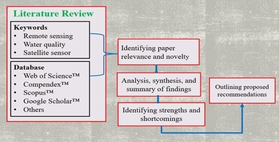
1. Introduction
2. Water Quality Monitoring
2.1. Water Resources Degradation
2.2. Water Quality Parameters
2.3. Remote Sensing
2.3.1. Remote Sensing Systems
Microwave Remote Sensing
Optical Remote Sensing
Spectral Imaging
Airborne and Spaceborne Sensors
- Spectral and spatial resolutions: airborne sensors have higher spectral and spatial resolutions making them appropriate for the measurement of WQPs. Hyperspectral airborne sensors produce images that allow for more detailed spatial and spectral models for the accurate classification of an image.
- Flexibility in terms of configuration: airborne sensors have higher flexibility in terms of their configuration in terms of spectral range, number bands, and wavelength. The time of survey for any project work is not fixed. There is no repeat cycle as in the case of spaceborne sensors.
- Larger geographic areas: airborne sensors can operate at higher altitudes covering a larger geographic area, and hence are suitable for regional water quality monitoring.
- Monitoring of small water bodies: airborne sensors can assess small water bodies including rivers, estuaries, ponds, and tributaries.
- Greater planning: there is a need for greater planning ahead before the airborne survey. Considerations need to be made for external factors including air traffic, weather, flight line orientations, and solar radiation.
- Cost: airborne surveys are more cost-intensive compared with spaceborne sensors. Sensitive detectors, large data storage capacity, and fast computers are needed for the image processing of airborne sensors.
- Altitude: airborne sensors usually cover smaller areas as compared to spaceborne sensors due to the lower altitude of image acquisition.
- Cost: spaceborne sensors produce images at typically zero to little cost and can be used for large-scale monitoring of water quality.
- Less complexity with image processing: compared to airborne sensors, processing the spaceborne image is less complex.
- Multi-temporal studies: spaceborne sensors have a revisit frequency ranging from daily to monthly making them useful for multi-temporal scale monitoring of the trends and variations in WQPs.
- Coverage of large geographic areas: spaceborne sensors can cover large geographic areas making them suitable for moderate, regional, and global water quality monitoring.
- Cloud constraints: spaceborne sensors are faced with enormous limitations when a project requires a cloud-free image.
- Overestimation of water parameters: empirical and semi-empirical approaches in analyzing multispectral images by spaceborne sensors may lead to overestimations at areas where there is a contribution of reflectance from the bottom to the water leaving reflectance.
- High-resolution images acquired are costly. The limitation with coverage: there is a limitation with coverage of the electromagnetic spectrum by spaceborne sensors. Some bands such as middle infrared and thermal bands may not be covered, which may impact the accuracy of the estimation of WQPs.
- Airborne Visible Infrared Imaging Spectrometer (AVIRIS): This sensor is manufactured by NASA Jet Propulsion Lab with a hyperspectral image with 224 bands. This image has a 17 m resolution with a spectral range of 0.40–2.50 µm. The sensor utilizes the whiskbroom scan system.
- Hyperspectral Digital Imagery Collection Experiment (HYDICE). This sensor is manufactured by the Naval Research Lab with a pushbroom scan system. This is also a hyperspectral image with 210 bands with a spectral range of 0.40–2.50 µm and a spatial resolution of 0.8 to 4 m.
- Airborne Prism Experiment (APEX). This sensor is manufactured by VITO and produces up to 300 hyperspectral bands with a pushbroom scan system. The spatial resolution of images produced ranges from 2 to 5 m and the spectral range of 0.38–2.50 µm.
- Compact Airborne Spectrographic Imager (CASI-1500). This sensor is manufactured by ITRES Research Limited and produces up to 228 hyperspectral bands of spectral range 0.40–1.00 µm and a spatial resolution of 0.5–3 m with a pushbroom scan system.
- Multispectral Infrared and Visible Imaging Spectrometer (MIVIS): This sensor is manufactured by Daedalus Enterprise Inc., USA, and produces multispectral images of visible, near-infrared, mid-infrared, and thermal bands. The sensor operates on the whiskbroom scan systems with resolutions ranging from 3 to 8 m depending on the altitude.
- Airborne Imaging Spectrometer (AISA). This sensor is manufactured by Spectral Imaging and produces hyperspectral bands of up to 288 bands with a spatial resolution of 0.43 to 0.9 µm. Images have a spatial resolution of 1 m. The sensor operates on the pushbroom scan system.
- Digital Airborne Imaging Spectrometer (DAIS 7915). This sensor is manufactured by GER Corporation and produces hyperspectral bands with a spatial resolution of 0.43 to 12.30 µm. Images have a spatial resolution of 3–20 m depending on the altitude. The sensor operates on the whiskbroom scan system.
- Landsat satellite images: Landsat programs are joint efforts of the USGS and NASA for Earth Observation and have been in existence since 1972. Landsat images have been used by stakeholders in many applications such as land use planning, natural resources management, public safety, climate research, natural disaster management, home security, and agriculture, among others [114]. The Landsat 8 Operational Land Imager (OLI), Landsat 7 Enhanced Thematic Mapper (ETM+), and Landsat 5 TM have all been used in water quality monitoring efforts. The Landsat 9 sensor has a 14-bit quantization, which can differentiate 16,384 shades, i.e., a brightness uncertainty of ±0.006%) at a given wavelength. The Landsat 8 OLI sensor captures data over a 12-bit instrument with improved precision in radiometry. The sensor captures images with the overall improvement in the signal-to-noise ratio, which translates to 4096 grey levels (i.e., a brightness uncertainty of ±0.024%). Landsat 1 to 7 sensors capture data with 256 grey levels (i.e., a brightness uncertainty of ±0.4%) over an 8-bit dynamic range. The Landsat 8 OLI data with 12-bit are scaled to 16-bit and made available in the form of level-1 data products. These are scaled to 55,000 grey levels from the 65,536 grey levels, which can be subsequently rescaled with radiometric coefficients, which come with the product metadata file (MTL file). The rescaling is performed to the Top of the Atmosphere (TOA) reflectance and or radiance [115,116].
- Landsat 9 OLI/TIRS: The Landsat 9 sensor is the latest series of Earth-observing satellites launched on 27 September 2021, and its data are publicly available (Yang et al., 2022). The sensor was launched from Vandenberg Air Force Base, California, USA, onboard a United Launched Alliance Atlas V 401 rocket and it is an improved replica of the Landsat 8 sensor. It carries the Operational Land Imager 2 (OLI-2), built by Ball Aerospace & Technologies Cooperation, Boulder, CO, USA, and the Thermal Infrared Sensor 2 (TIRS-2), built at the NASA Goddard Space Flight Center, Greenbelt, MA, USA. The Landsat 9 OLI-2 provides images consistent with Landsat 8 spectral, spatial, geometric, and radiometric qualities. It has nine spectral bands over a 185 km swath of 30 m resolutions for all bands except for the panchromatic band, which is 15 m, at a maximum ground sampling distance (GSD) both in and cross tracks. Landsat 9 offers a 16-day revisit earth coverage and an 8-day offset with Landsat 8. It acquires more than 700 scenes per day [117]. The sensor was launched to continue with the collection, distribution, and archival of multispectral imagery offering users the synoptic, global, and repetitive coverage of the Earth’s surface for the detection of natural and human-induced changes on a spatiotemporal scale [117].
- Landsat 8 OLI/TIRS: The Landsat 8 carries the OLI and Thermal Infrared Sensor (TIRS) sensors. It was previously called the Landsat Data Continuity Mission (LDCM) and was launched on an Atlas-V rocket from Vandenberg Air Force Base, California, USA, on 11 February 2013. Landsat 8 OLI has nine spectral bands. Studies have used some of these bands and their combinations for water quality estimations. All the bands have a spatial resolution of 30 m, except band 8 with a finer spatial resolution of 15 m. A 30 m resolution means each pixel of the image provides an average reflectance value recorded of an area of 900 m2 (30 m by 30 m) [89]. Landsat 8 OLI is available by the United States Geological Survey (USGS) on 16 days of repeat time with an equatorial crossing time of 10:00 am ± 15 min mean local time [116,118]. The Landsat 8 OLI sensor acquires around 740 scenes in a day on the Worldwide Reference System-2 (WRS-2) path/row system. It has a swath overlap that varies from 7% at the equator to about 85% at extreme latitudes. Each scene size is 114 mi × 112 mi [116].
- Landsat 7 Enhanced Thematic Mapper (ETM+): The Landsat 7 was launched from Vandenberg Air Force Base, California, USA, on 15 April 1999, with a repeat cycle of 16 days. The Landsat 7 carries an improved version of the Thematic Mapper I instrument, which was onboard Landsat 4 and 5. ETM+ sensor Landsat 7 ETM+ data collected since 2003 have gaps caused by the Scan Line Corrector (SLC) failure. Each scene of this image is 185 km wide. Landsat 7 images are delivered in 8 bits with 256 grey levels [119]. Landsat 7 ETM+ is also available by the USGS on 16 days repeat time with an equatorial crossing time of 10:00 am ± 15 mean local time [120,121]. All the bands have a 30 m resolution, except band 6 and band 8 with 60 m and 15 m resolutions, respectively [119].
- Landsat 5 TM: These data sets consist of seven bands with 30 m spatial resolutions for all bands except band 6, which has 120 m resolutions and, in turn, is resampled to 30 m. This sensor was launched on March 1, 1984, from Vandenberg Air Force Base in California, USA, with its data products quantized to eight bits. It carries both the Multispectral Scanner (MSS) and the TM instruments. The sensor delivered data for close to 29 years and was retired on 5 June 2013 [121,122,123]. Landsat 5 TM images are delivered in 8 bits with 256 grey levels [124].
- RapidEye images: The RapidEye sensor was launched on 29 August 2008, with a 6.5 m spatial resolution. This sensor produces images used in a variety of applications, including agriculture, engineering, construction, mining, and cartography. The RapidEye sensor has five (5) spectral bands and a spacecraft lifetime of 7 years. It has a 5.5-day revisit time off-nadir and at nadir, respectively, and an approximate equator crossing time of 11:00 am local time. It has a swath width of 77 km, a camera dynamic range of 12 bits, and an image capture capacity of 5 million km2/day. The RapidEye constellation was retired on 31 March 2020.
- Advanced Spaceborne Thermal Emission and Reflection Radiation (ASTER): The National Aeronautics and Space Administration (NASA) launched the ASTER sensor on the Terra satellite in December 1999. It has an equatorial crossing time at 10:30 a.m. local time with 16 days of repeat time. It has a resolution of 15, 30, and 90 m depending on the bands with quantization levels of 8 bits for the 15 and 30 m resolution bands and 12 bits for the 90 m resolution. ASTER is a collaboration between NASA, Japan’s Economy Ministry, Trade and Industry, and Japan Space System. ASTER data are used in the mapping of land surface temperature, elevation, and reflectance Additionally, they are used in applied geology, soils, hydrology, ecosystems dynamics, and land cover change studies [125]. ASTER is made of different subsystems, namely, the Visible and Near-infrared (VNIR), SWIR, and Thermal Infrared (TIR). Each of these subsystems collects data in a separate set of wavebands with each set having its spatial resolution. The sensor has fourteen different bands with varying spatial resolutions for each subsystem.
- Moderate Resolution Imaging Spectroradiometer (MODIS): The first MODIS instrument was launched aboard NASA Terra in December 1999, with the second instrument launched in May 2002 aboard the NASA Aqua platform. These data have been available since February 2000 and June 2002, respectively, for the Terra and Aqua platforms. The Terra and Aqua satellite platforms have local equatorial crossing times at 10:30 a.m. and 1:30 p.m., respectively [126,127]. The MODIS sensor has a repeat cycle of 16 days and 12-bit quantization. MODIS data consist of 36 spectral bands with varying wavelengths and spatial resolutions. The MODIS sensor has 250 m spatial resolution for bands 1 and 2, 500 m for bands 3–7, and 1 km for bands 8–36. The wavelength of bands 1 to 19 ranges from 405 to 2155 nm, with bands 20–36 ranging from 3.66 to 14.28 µm. MODIS images are utilized in studying and understanding environmental phenomena, and dynamic variations in inland, ocean, and the lower atmosphere [127]. Although the MODIS data with medium resolution (i.e., 250 and 500 m resolutions) were originally designed for land studies and cloud monitoring and have lower sensitivities than MODIS ocean bands. The moderate resolution MODIS was compared with Landsat 7 ETM+ and Coastal Zone Color Scanner (CZCS), and SeaWiFS in a study and were found to provide sufficient sensitivity for water application data. The MODIS Ocean band (i.e., 1 km resolution) was found to be 3 to 6 times more sensitive than the SeaWiFS bands, which makes it possible for them to detect subtle ocean features. Compared to Landsat 7 ETM+ bands, the moderate resolution bands of MODIS (250 and 500 m) are found to be more sensitive with nearly twice the sensitivity of CZCS blue-green bands. MODIS moderate resolution bands are hence expected to be as useful as CZCS for coastal ocean studies [128].
- Sentinel-2 MSI: Several group efforts led by the Airbus Defense resulted in the design and building of the Sentinel-2 sensor. The Sentinel-2 satellites are a constellation of the European Space Agency (ESA) and were launched on multispectral scanners [129]. The Sentinel-2 sensor comprises two identical satellites, namely, Sentinel-2A and Sentinel-2B, in the same sun-synchronous orbit. These satellites are separated at an angle of 180° from each other with a mean orbital altitude of 786 km. The crossing time of the sentinel sensor at the descending node is 10:30 am Mean Local Solar Time (MLST). The sensors were launched on a Vega rocket from Kourou in French Guiana on 23 June 2015, and 7 March 2017, respectively, for the Sentinel 2A and 2B [130,131]. Sentinel-2 images are used in the study of water quality, impervious surface mapping, monitoring of land ecosystems and land-use land cover (LULC), forest management, agriculture, and disaster mapping [129,131,132,133]. The sensor has 10 days of revisit time with one satellite and 5 days of revisit time with the two satellites, at the equator under cloud-free conditions [134]. The sensor has a swath width of 290 km. The Sentinel-2 has a 12-bit radiometric resolution and spatial resolution ranging from 10 m for bands 2, 3, 4, and 8; 20 m for bands 5, 6, 7, 8a, 11, and 12; to 60 m for bands 1, 9, and 10, with wavelengths varying from 442.7 to 2202.4 nm for band 1 to 11, respectively [113].
2.3.2. Characterization of Water Quality Parameters
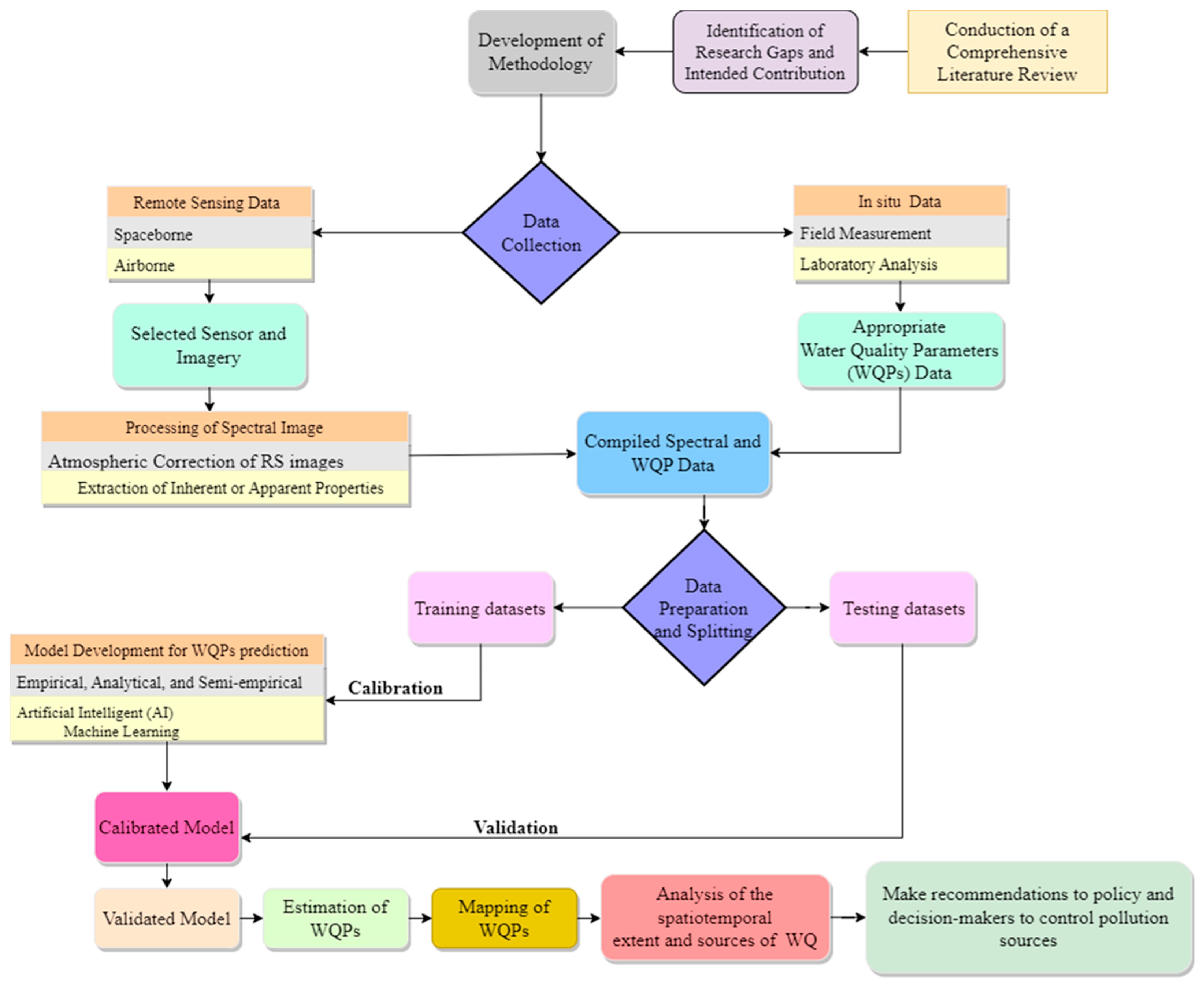
2.3.3. Remote Sensing Principles in Water Quality Monitoring
2.3.4. RS Retrieval of Water Quality Parameters
- Empirical method: this approach utilizes statistical relationships derived between measured RS spectral values and measured water quality. The relationship is established using regression techniques. Estimations performed by empirical models need in situ data as many parameters are likely to change between RS missions. The empirical methods are simple and easier approaches to the retrieval of water quality.
- Analytical method: the IOPs and AOPs are used to model the reflectance. Physical relationships are then derived between the WQP, the underwater light field, and the remotely sensed radiance. This method involves the use of bio-optical and transmission models to simulate the propagation of light in water bodies and the relationship between the WQP and reflection. Parameters such as TDS are, however, determined due to their association with other colored WQPs. Salinity is only determined in microwave bands.
- The semi-empirical methods: this approach is the combination of the empirical and analytical methods for the retrieval of WQPs. In this method, the spectral characteristics of the parameters are known. Here, the appropriate combination of wavebands is used as correlates. The spectral radiance is recalculated to above the surface irradiance reflectance, and then through regression techniques related to the WQP.
- Artificial Intelligence (AI) methods: this is an implicit algorithm approach that differs from the three other approaches outlined i–iii. The complications from various water surfaces, WQP combinations, and sediment deposits will mean the need to use implicit algorithms for the retrieval of WQPs. AI applications capture both linear and nonlinear relationships compared with conventional statistical approaches. Studies have applied various AI applications including the neural network (NN), which is non-linear, as compared to a linear MLR model and SVM in water quality retrieval, and produced satisfactory results. ML models such as the ANN outperforms regression models such as MLR models [48,146].
2.3.5. Detection of Optically Active Parameters
2.3.6. Detection of Optically Inactive Parameters
2.3.7. Remote Sensing Applications in Water Quality Monitoring
3. Strengths and Shortcomings of RS Applications
3.1. Strengths
3.2. Limitations
4. Summary and Recommendations
Author Contributions
Funding
Data Availability Statement
Conflicts of Interest
References
- Chen, X.; Liu, L.; Zhang, X.; Li, J.; Wang, S.; Liu, D.; Duan, H.; Song, K. An Assessment of Water Color for Inland Water in China Using a Landsat 8-Derived Forel-Ule Index and the Google Earth Engine Platform. IEEE J. Sel. Top. Appl. Earth Obs. Remote Sens. 2021, 14, 5773–5785. [Google Scholar] [CrossRef]
- Hajigholizadeh, M.; Moncada, A.; Kent, S.; Melesse, A.M. Land–lake linkage and remote sensing application in water quality monitoring in lake okeechobee, florida, usa. Land 2021, 10, 147. [Google Scholar] [CrossRef]
- Schaeffer, B.A.; Schaeffer, K.G.; Keith, D.; Lunetta, R.S.; Conmy, R.; Gould, R.W. Barriers to adopting satellite remote sensing for water quality management. Int. J. Remote Sens. 2013, 34, 7534–7544. [Google Scholar] [CrossRef]
- Uudeberg, K.; Aavaste, A.; Kõks, K.-L.; Ansper, A.; Uusõue, M.; Kangro, K.; Ansko, I.; Ligi, M.; Toming, K.; Reinart, A. Optical Water Type Guided Approach to Estimate Optical Water Quality Parameters. Remote Sens. 2020, 12, 931. [Google Scholar] [CrossRef] [Green Version]
- Yang, H.; Kong, J.; Hu, H.; Du, Y.; Gao, M.; Chen, F. A Review of Remote Sensing for Water Quality Retrieval: Progress and Challenges. Remote Sens. 2022, 14, 1770. [Google Scholar] [CrossRef]
- McCarthy, M.J.; Colna, K.E.; El-Mezayen, M.M.; Laureano-Rosario, A.E.; Méndez-Lázaro, P.; Otis, D.B.; Toro-Farmer, G.; Vega-Rodriguez, M.; Muller-Karger, F.E. Satellite Remote Sensing for Coastal Management: A Review of Successful Applications. Environ. Manag. 2017, 60, 323–339. [Google Scholar] [CrossRef]
- Allan, M.G.; Hamilton, D.P.; Hicks, B.J.; Brabyn, L. Landsat remote sensing of chlorophyll a concentrations in central North Island lakes of New Zealand. Int. J. Remote Sens. 2011, 32, 2037–2055. [Google Scholar] [CrossRef]
- Gholizadeh, M.H.; Melesse, A.M.; Reddi, L. Spaceborne and airborne sensors in water quality assessment. Int. J. Remote Sens. 2016, 37, 3143–3180. [Google Scholar] [CrossRef]
- Adjovu, G.E.; Stephen, H.; Ahmad, S. Monitoring of Total Dissolved Solids Using Remote Sensing Band Reflectance and Salinity Indices: A Case Study of the Imperial County Section, AZ-CA, of the Colorado River. World Environ. Water Resour. Congr. 2022, 2022, 1132. [Google Scholar] [CrossRef]
- Pizani, F.M.C.; Maillard, P.; Ferreira, A.F.F.; De Amorim, C.C. Estimation of Water Quality in a Reservoir from Sentinel-2 MSI amd Landsat-8 OLI Sensors. ISPRS Ann. Photogramm. Remote Sens. Spat. Inf. Sci. 2020, V-3-2020, 401–408. [Google Scholar] [CrossRef]
- Zhou, Y.; Dong, J.; Xiao, X.; Xiao, T.; Yang, Z.; Zhao, G.; Zou, Z.; Qin, Y. Open surface water mapping algorithms: A comparison of water-related spectral indices and sensors. Water 2017, 9, 256. [Google Scholar] [CrossRef]
- Zhou, B.; Shang, M.; Wang, G.; Zhang, S.; Feng, L.; Liu, X.; Wu, L.; Shan, K. Distinguishing two phenotypes of blooms using the normalised difference peak-valley index (NDPI) and Cyano-Chlorophyta index (CCI). Sci. Total Environ. 2018, 628–629, 848–857. [Google Scholar] [CrossRef] [PubMed]
- Gallagher, L.C. Hyperspectral Remote Sensing of Suspended Minerals, Chlorophyll and Coloured Dissolved Organic Matter in Coastal and Inland Waters, British Columbia, Canada. Mater’s Thesis, University of Victoria, Victoria, BC, Canada, 2004. [Google Scholar]
- Abbas, A.; Khan, S. Using remote sensing techniques for appraisal of irrigated soil salinity. In Land, Water Environment Management Integrated Systems for Sustainability, Proceedings of the MODSIM 2007 International Congress on Modelling and Simulation, Canberra, Australia, 10–13 December 2007; Modelling and Simulation Society of Australia and New Zealand: Christchurch, New Zealand, 2007; pp. 2632–2638. [Google Scholar]
- Deutsch, E.S.; Alameddine, I.; El-Fadel, M. Monitoring water quality in a hypereutrophic reservoir using Landsat ETM+ and OLI sensors: How transferable are the water quality algorithms? Environ. Monit. Assess. 2018, 190, 141. [Google Scholar] [CrossRef]
- Gholizadeh, M.H.; Melesse, A.M.; Reddi, L. A comprehensive review on water quality parameters estimation using remote sensing techniques. Sensors 2016, 16, 1298. [Google Scholar] [CrossRef] [PubMed] [Green Version]
- Usali, N.; Ismail, M.H. Use of Remote Sensing and GIS in Monitoring Water Quality. J. Sustain. Dev. 2010, 3, 228–238. [Google Scholar] [CrossRef]
- Dube, T.; Mutanga, O.; Seutloali, K.; Adelabu, S.; Shoko, C. Water quality monitoring in sub-Saharan African lakes: A review of remote sensing applications. Afr. J. Aquat. Sci. 2015, 40, 1–7. [Google Scholar] [CrossRef]
- Avdan, Z.Y.; Kaplan, G.; Goncu, S.; Avdan, U. Monitoring the water quality of small water bodies using high-resolution remote sensing data. ISPRS Int. J. Geo-Inf. 2019, 8, 553. [Google Scholar] [CrossRef] [Green Version]
- Olmanson, L.G.; Brezonik, P.L.; Bauer, M.E. Evaluation of medium to low resolution satellite imagery for regional lake water quality assessments. Water Resour. Res. 2011, 47, W09515. [Google Scholar] [CrossRef] [Green Version]
- Alparslan, E.; Aydöner, C.; Tufekci, V.; Tüfekci, H. Water quality assessment at Ömerli Dam using remote sensing techniques. Environ. Monit. Assess. 2007, 135, 391–398. [Google Scholar] [CrossRef]
- D’Ortenzio, F.; Marullo, S.; Ragni, M.; D’Alcalà, M.R.; Santoleri, R. Validation of empirical SeaWiFS algorithms for chlorophyll-a retrieval in the Mediterranean Sea: A case study for oligotrophic seas. Remote Sens. Environ. 2002, 82, 79–94. [Google Scholar] [CrossRef]
- Gitelson, A.A.; Dall’Olmo, G.; Moses, W.; Rundquist, D.C.; Barrow, T.; Fisher, T.R.; Gurlin, D.; Holz, J. A simple semi-analytical model for remote estimation of chlorophyll-a in turbid waters: Validation. Remote Sens. Environ. 2008, 112, 3582–3593. [Google Scholar] [CrossRef]
- He, W.; Chen, S.; Liu, X.; Chen, J. Water quality monitoring in a slightly-polluted inland water body through remote sensing—Case study of the Guanting Reservoir in Beijing, China. Front. Environ. Sci. Eng. China 2008, 2, 163–171. [Google Scholar] [CrossRef]
- Isidro, C.M.; McIntyre, N.; Lechner, A.M.; Callow, I. Quantifying suspended solids in small rivers using satellite data. Sci. Total Environ. 2018, 634, 1554–1562. [Google Scholar] [CrossRef] [PubMed]
- Karami, J.; Alimohammadi, A.; Modabberi, S. Analysis of the spatio-temporal patterns of water pollution and source contribution using the MODIS sensor products and multivariate statistical techniques. IEEE J. Sel. Top. Appl. Earth Obs. Remote Sens. 2012, 5, 1243–1255. [Google Scholar] [CrossRef]
- Mabwoga, S.O.; Chawla, A.; Thukral, A.K. Assessment of water quality parameters of the Harike wetland in India, a Ramsar site, using IRS LISS IV satellite data. Environ. Monit. Assess. 2010, 170, 117–128. [Google Scholar] [CrossRef]
- Maliki, A.A.A.; Chabuk, A.; Sultan, M.A.; Hashim, B.M.; Hussain, H.M.; Al-Ansari, N. Estimation of Total Dissolved Solids in Water Bodies by Spectral Indices Case Study: Shatt al-Arab River. Water Air Soil Pollut. 2020, 231, 482. [Google Scholar] [CrossRef]
- Morel, A.; Bélanger, S. Improved detection of turbid waters from ocean color sensors information. Remote Sens. Environ. 2006, 102, 237–249. [Google Scholar] [CrossRef]
- Pereira, O.J.R.; Merino, E.R.; Montes, C.R.; Barbiero, L.; Rezende-Filho, A.T.; Lucas, Y.; Melfi, A.J. Estimating water pH using cloud-based landsat images for a new classification of the Nhecolândia Lakes (Brazilian Pantanal). Remote Sens. 2020, 12, 1090. [Google Scholar] [CrossRef] [Green Version]
- Petus, C.; Chust, G.; Gohin, F.; Doxaran, D.; Froidefond, J.M.; Sagarminaga, Y. Estimating turbidity and total suspended matter in the Adour River plume (South Bay of Biscay) using MODIS 250-m imagery. Cont. Shelf Res. 2010, 30, 379–392. [Google Scholar] [CrossRef] [Green Version]
- Toming, K.; Kutser, T.; Tuvikene, L.; Viik, M.; Nõges, T. Dissolved organic carbon and its potential predictors in eutrophic lakes. Water Res. 2016, 102, 32–40. [Google Scholar] [CrossRef]
- Ansper, A.; Alikas, K. Retrieval of chlorophyll a from Sentinel-2 MSI data for the European Union water framework directive reporting purposes. Remote Sens. 2019, 11, 64. [Google Scholar] [CrossRef] [Green Version]
- Gómez, J.A.D.; Alonso, C.A.; García, A.A. Remote sensing as a tool for monitoring water quality parameters for Mediterranean Lakes of European Union water framework directive (WFD) and as a system of surveillance of cyanobacterial harmful algae blooms (SCyanoHABs). Environ. Monit. Assess. 2011, 181, 317–334. [Google Scholar] [CrossRef] [PubMed]
- Potes, M.; Costa, M.J.; Salgado, R. Satellite remote sensing of water turbidity in Alqueva reservoir and implications on lake modelling. Hydrol. Earth Syst. Sci. 2012, 16, 1623–1633. [Google Scholar] [CrossRef] [Green Version]
- Adjovu, G.E.; Ahmad, S.; Stephen, H. Analysis of Suspended Material in Lake Mead Using Remote Sensing Indices. World Environ. Water Resour. Congr. 2021, 2021, 754–768. [Google Scholar] [CrossRef]
- Dekker, A.G.; Hestir, E.L. Evaluating the Feasibility of Systematic Inland Water Quality Monitoring with Satellite Remote Sensing; Water for a Healthy Country WIRADA; CSIRO: Canberra, Australia, 2012; p. 105. [Google Scholar]
- AL-Fahdawi, A.A.H.; Rabee, A.M.; Al-Hirmizy, S.M. Water quality monitoring of Al-Habbaniyah Lake using remote sensing and in situ measurements. Environ. Monit. Assess. 2015, 187, 367. [Google Scholar] [CrossRef] [PubMed]
- Karagiannis, I.C.; Soldatos, P.G. Water desalination cost literature: Review and assessment. Desalination 2008, 223, 448–456. [Google Scholar] [CrossRef]
- Dey, J.; Vijay, R. A critical and intensive review on assessment of water quality parameters through geospatial techniques. Environ. Sci. Pollut. Res. 2021, 28, 41612–41626. [Google Scholar] [CrossRef]
- Dörnhöfer, K.; Oppelt, N. Remote sensing for lake research and monitoring—Recent advances. Ecol. Indic. 2016, 64, 105–122. [Google Scholar] [CrossRef]
- Karaoui, I.; Arioua, A.; Boudhar, A.; Hssaisoune, M.; El Mouatassime, S.; Ouhamchich, K.A.; Elhamdouni, D.; Idrissi, A.E.A.; Nouaim, W. Evaluating the potential of Sentinel-2 satellite images for water quality characterization of artificial reservoirs: The Bin El Ouidane Reservoir case study (Morocco). Meteorol. Hydrol. Water Manag. 2019, 7, 31–39. [Google Scholar]
- Nath, R.K.; Deb, S.K. Water-Body Area Extraction From High Resolution Satellite Images-An Introduction, Review, and Comparison. Int. J. Image Process. 2010, 3, 353–372. [Google Scholar]
- Palmer, S.C.J.; Kutser, T.; Hunter, P.D. Remote sensing of inland waters: Challenges, progress and future directions. Remote Sens. Environ. 2015, 157, 1–8. [Google Scholar] [CrossRef] [Green Version]
- Song, K. Water quality monitoring using Landsat Themate Mapper data with empirical algorithms in Chagan Lake, China. J. Appl. Remote Sens. 2011, 5, 053506. [Google Scholar] [CrossRef]
- Buma, W.G.; Lee, S.I. Evaluation of Sentinel-2 and Landsat 8 images for estimating Chlorophyll-a concentrations in Lake Chad, Africa. Remote Sens. 2020, 12, 2437. [Google Scholar] [CrossRef]
- Ogashawara, I.; Mishra, D.R.; Gitelson, A.A. Remote Sensing of Inland Waters: Background and Current State-of-the-Art; Elsevier Inc.: Amsterdam, The Netherlands, 2017. [Google Scholar] [CrossRef]
- Vakili, T.; Amanollahi, J. Determination of optically inactive water quality variables using Landsat 8 data: A case study in Geshlagh reservoir affected by agricultural land use. J. Clean. Prod. 2020, 247, 119134. [Google Scholar] [CrossRef]
- Zhang, K.; Amineh, R.K.; Dong, Z.; Nadler, D. Microwave Sensing of Water Quality. IEEE Access 2019, 7, 69481–69493. [Google Scholar] [CrossRef]
- Salmaso, N.; Mosello, R. Limnological research in the deep southern subalpine lakes: Synthesis, directions and perspectives. Adv. Oceanogr. Limnol. 2010, 1, 29–66. [Google Scholar] [CrossRef]
- De Vlaming, V.; DiGiorgio, C.; Fong, S.; Deanovic, L.; Carpio-Obeso, M.D.L.P.; Miller, J.; Miller, M.; Richard, N. Irrigation runoff insecticide pollution of rivers in the Imperial Valley, California (USA). Environ. Pollut. 2004, 132, 213–229. [Google Scholar] [CrossRef]
- Kimbrough, R.A.; Litke, D.W. Pesticides in streams draining agricultural and urban areas in Colorado. Environ. Sci. Technol. 1996, 30, 908–916. [Google Scholar] [CrossRef] [Green Version]
- Stout, W.L.; Fales, S.L.; Muller, L.D.; Schnabel, R.R.; Elwinger, G.F.; Weaver, S.R. Assessing the effect of management intensive grazing on water quality in the northeast U.S. J. Soil Water Conserv. 2000, 55, 238–243. [Google Scholar]
- Schliemann, S.A.; Grevstad, N.; Brazeau, R.H. Water quality and spatio-temporal hot spots in an effluent-dominated urban river. Hydrol. Process. 2021, 35, e14001. [Google Scholar] [CrossRef]
- Masocha, M.; Murwira, A.; Magadza, C.H.D.; Hirji, R.; Dube, T. Remote sensing of surface water quality in relation to catchment condition in Zimbabwe. Phys. Chem. Earth 2017, 100, 13–18. [Google Scholar] [CrossRef]
- Mueller, J.S.; Grabowski, T.B.; Brewer, S.K.; Worthington, T.A. Effects of temperature, total dissolved solids, and total suspended solids on survival and development rate of larval Arkansas River shiner. J. Fish Wildl. Manag. 2017, 8, 79–88. [Google Scholar] [CrossRef] [Green Version]
- Fant, C.; Srinivasan, R.; Boehlert, B.; Rennels, L.; Chapra, S.C.; Strzepek, K.M.; Corona, J.; Allen, A.; Martinich, J. Climate change impacts on us water quality using two models: HAWQS and US basins. Water 2017, 9, 118. [Google Scholar] [CrossRef] [Green Version]
- Tran, P.H.; Nguyen, A.K.; Liou, Y.-A.; Hoang, P.P.; Thanh, H.N. Estimation of Salinity Intrusion by Using Landsat 8 OLI Data in The Mekong Delta, Vietnam. Prog. Earth Planet. Sci. 2020, 7, 1. [Google Scholar] [CrossRef] [Green Version]
- Hannah, D.M.; Brown, L.E.E.E.; Milner, A.M. Integrating climate—Hydrology—Ecology for alpine river systems. Aquat. Conserv. Mar. Freshw. Ecosyst. 2007, 656, 636–656. [Google Scholar] [CrossRef]
- Gunatilaka, A.; Moscetta, P.; Sanfilippo, L. Recent Advancements in Water Quality Monitoring-the use of miniaturized sensors and novel analytical measuring techniques for in-situ and on-line real time. In Proceedings of the International Workshop on Monitoring and Sensor for Water Pollution Control, Beijing, China, 13–14 June 2007; pp. 33–43. [Google Scholar]
- Oun, A.; Kumar, A.; Harrigan, T.; Angelakis, A.; Xagoraraki, I. Effects of biosolids and manure application on microbial water quality in rural areas in the US. Water 2014, 6, 3701–3723. [Google Scholar] [CrossRef] [Green Version]
- Fujioka, R.S.; Solo-Gabriele, H.M.; Byappanahalli, M.N.; Kirs, M. U.S. recreational water quality criteria: A vision for the future. Int. J. Environ. Res. Public Health 2015, 12, 7752–7776. [Google Scholar] [CrossRef] [Green Version]
- Vedwan, N.; Ahmad, S.; Miralles-Wilhelm, F.; Broad, K.; Letson, D.; Podesta, G. Institutional evolution in Lake Okeechobee Management in Florida: Characteristics, impacts, and limitations. Water Resour. Manag. 2008, 22, 699–718. [Google Scholar] [CrossRef]
- Lee, S.; Ahn, K.H. Monitoring of COD as an organic indicator in waste water and treated effluent by fluorescence excitation-emission (FEEM) matrix characterization. Water Sci. Technol. 2004, 50, 57–63. [Google Scholar] [CrossRef]
- El Serafy, G.Y.H.; Schaeffer, B.A.; Neely, M.-B.; Spinosa, A.; Odermatt, D.; Weathers, K.C.; Baracchini, T.; Bouffard, D.; Carvalho, L.; Conmy, R.N.; et al. Integrating Inland and Coastal Water Quality Data for Actionable Knowledge. Remote Sens. 2021, 13, 2899. [Google Scholar] [CrossRef]
- Mondal, K.C.; Rathod, K.G.; Joshi, H.M.; Mandal, H.S.; Khan, R.; Rajendra, K.; Mawale, Y.K.; Priya, K.; Jhariya, D.C. Impact of land-use and land-cover change on groundwater quality and quantity in the Raipur, Chhattisgarh, India: A remote sensing and GIS approach. IOP Conf. Ser. Earth Environ. Sci. 2020, 597, 012011. [Google Scholar] [CrossRef]
- Lin, W.; Li, Z. Detection and quantification of trace organic contaminants in water using the FT-IR-attenuated total reflectance technique. Anal. Chem. 2010, 82, 505–515. [Google Scholar] [CrossRef] [PubMed]
- Tsuchiya, Y. Organical Chemicals As Contaminants of Water Bodies and Drinking Water. Water Qual. Stand. 2010, II, 150–171. [Google Scholar]
- Ibrahim, N.; Aziz, H.A. Trends on Natural Organic Matter in Drinking Water Sources and its Treatment. Int. J. Sci. Res. Environ. Sci. 2014, 2, 94–106. [Google Scholar] [CrossRef]
- Christian, E.; Batista, J.R.; Gerrity, D. Use of COD, TOC, and Fluorescence Spectroscopy to Estimate BOD in Wastewater. Water Environ. Res. 2016, 89, 168–177. [Google Scholar] [CrossRef]
- Hu, H.-Y.; Du, Y.; Wu, Q.Y.; Zhao, X.; Tang, X.; Chen, Z. Differences in dissolved organic matter between reclaimed water source and drinking water source. Sci. Total Environ. 2016, 551–552, 133–142. [Google Scholar] [CrossRef]
- Cao, F.; Tzortziou, M.; Hu, C.; Mannino, A.; Fichot, C.G.; Del Vecchio, R.; Najjar, R.G.; Novak, M. Remote sensing retrievals of colored dissolved organic matter and dissolved organic carbon dynamics in North American estuaries and their margins. Remote Sens. Environ. 2018, 205, 151–165. [Google Scholar] [CrossRef]
- Kutser, T.; Pierson, D.C.; Tranvik, L.; Reinart, A.; Sobek, S.; Kallio, K. Using satellite remote sensing to estimate the colored dissolved organic matter absorption coefficient in lakes. Ecosystems 2005, 8, 709–720. [Google Scholar] [CrossRef]
- Al-Kharusi, E.S.; Tenenbaum, D.E.; Abdi, A.M.; Kutser, T.; Karlsson, J.; Bergström, A.-K.; Berggren, M. Large-Scale Retrieval of Coloured Dissolved Organic Matter in Northern Lakes Using Sentinel-2 Data. Remote Sens. 2020, 12, 157. [Google Scholar] [CrossRef] [Green Version]
- Rieger, L.; Langergraber, G.; Thomann, M.; Fleischmann, N.; Siegrist, H. Spectral in-situ analysis of NO2, NO3, COD, DOC and TSS in the effluent of a WWTP. Water Sci. Technol. 2004, 50, 143–152. [Google Scholar] [CrossRef]
- Cao, F.; Tzortziou, M. Capturing dissolved organic carbon dynamics with Landsat-8 and Sentinel-2 in tidally influenced wetland–estuarine systems. Sci. Total Environ. 2021, 777, 145910. [Google Scholar] [CrossRef]
- Wei, K.L.; Chen, M.; Wang, F.; Fang, Q. A rapid monitoring system for the determination of COD in waters based on ultrasonic assisted digestion and miniaturized spectral analytical system. Appl. Mech. Mater. 2013, 401–403, 1295–1300. [Google Scholar] [CrossRef]
- Denys, L. Incomplete spring turnover in small deep lakes in SE Michigan. McNair Sch. Res. J. 2010, 2, 133–144. [Google Scholar]
- Hasab, H.A.; Jawad, H.A.; Dibs, H.; Hussain, H.M.; Al-Ansari, N. Evaluation of Water Quality Parameters in Marshes Zone Southern of Iraq Based on Remote Sensing and GIS Techniques. Water. Air. Soil Pollut. 2020, 231, 183. [Google Scholar] [CrossRef] [Green Version]
- Fletcher, T.D.; Andrieu, H.; Hamel, P. Understanding, management and modelling of urban hydrology and its consequences for receiving waters: A state of the art. Adv. Water Resour. 2013, 51, 261–279. [Google Scholar] [CrossRef]
- Bonansea, M.; Ledesma, M.; Rodriguez, C.; Pinotti, L. Using new remote sensing satellites for assessing water quality in a reservoir. Hydrol. Sci. J. 2019, 64, 34–44. [Google Scholar] [CrossRef]
- Hidayati, N.F.; Rahman, M.; Fauzana, N.A.; Aisiah, S. Effectiveness of Chitosan To Reduce the Color Value, Turbidity, and Total Dissolved Solids in Shrimp-Washing Wastewater. Russ. J. Agric. Socio-Econ. Sci. 2021, 115, 82–88. [Google Scholar] [CrossRef]
- Mehdinejad, M.H.; Bina, B.; Nikaeen, M.; Attar, H.M. Effectiveness of natural and synthetic polyelectrolytes as coagulant aid in removal of turbidity from different turbid waters. J. Food Agric. Environ. 2013, 29, 261–266. [Google Scholar]
- Hellweger, F.L.; Schlosser, P.; Lall, U.; Weissel, J.K. Use of satellite imagery for water quality studies in New York Harbor. Estuar. Coast. Shelf Sci. 2004, 61, 437–448. [Google Scholar] [CrossRef]
- Chen, Q.; Zhang, Y.; Hallikainen, M. Water quality monitoring using remote sensing in support of the EU water framework directive (WFD): A case study in the Gulf of Finland. Environ. Monit. Assess. 2007, 124, 157–166. [Google Scholar] [CrossRef]
- Li, S.; Song, K.; Wang, S.; Liu, G.; Wen, Z.; Shang, Y.; Lyu, L.; Chen, F.; Xu, S.; Tao, H.; et al. Quantification of chlorophyll-a in typical lakes across China using Sentinel-2 MSI imagery with machine learning algorithm. Sci. Total Environ. 2021, 778, 146271. [Google Scholar] [CrossRef] [PubMed]
- Wei, J.; Lee, Z.; Ondrusek, M.; Mannino, A.; Tzortziou, M.; Armstrong, R. Spectral slopes of the absorption coefficient of colored dissolved and detrital material inverted from UV-visible remote sensing reflectance. J. Geophys. Res. Ocean. 2016, 121, 3010–3028. [Google Scholar] [CrossRef] [PubMed] [Green Version]
- Artlett, C.P.; Pask, H.M. New approach to remote sensing of temperature and salinity in natural water samples. Opt. Express 2017, 25, 2840. [Google Scholar] [CrossRef]
- Hossain, A.K.M.A.; Mathias, C.; Blanton, R. Remote sensing of turbidity in the tennessee river using landsat 8 satellite. Remote Sens. 2021, 13, 3785. [Google Scholar] [CrossRef]
- Li, R.; Li, J. Satellite Remote Sensing Technology for Lake Water Clarity Monitoring: An Overview. Environ. Inform. Arch. 2004, 2, 893–901. [Google Scholar]
- Devlin, M.J.; Petus, C.; Da Silva, E.; Tracey, D.; Wolff, N.H.; Waterhouse, J.; Brodie, J. Water quality and river plume monitoring in the Great Barrier Reef: An overview of methods based on ocean colour satellite data. Remote Sens. 2015, 7, 12909–12941. [Google Scholar] [CrossRef] [Green Version]
- Engman, E.T. Remote sensing in hydrology. Geophys. Monogr. Ser. 1998, 108, 165–177. [Google Scholar] [CrossRef]
- Varotsos, C.A.; Krapivin, V.F. Microwave Remote Sensing Tools in Environmental Science; Springer: Cham, Switzerland, 2020. [Google Scholar] [CrossRef]
- Quemada, C.; Pérez-Escudero, J.M.; Gonzalo, R.; Ederra, I.; Santesteban, L.G.; Torres, N.; Iriarte, J.C. Remote Sensing for Plant Water Content Monitoring: A Review. Remote Sensing 2021, 13, 2088. [Google Scholar] [CrossRef]
- Sagan, V.; Peterson, K.T.; Maimaitijiang, M.; Sidike, P.; Sloan, J.; Greeling, B.A.; Maalouf, S.; Adams, C. Monitoring inland water quality using remote sensing: Potential and limitations of spectral indices, bio-optical simulations, machine learning, and cloud computing. Earth-Sci. Rev. 2020, 205, 103187. [Google Scholar] [CrossRef]
- Zhou, X.; Liu, X.; Wang, X.; He, G.; Zhang, Y.; Wang, G.; Zhang, Z. Evaluation of surface reflectance products based on optimized 6s model using synchronous in situ measurements. Remote Sens. 2022, 14, 83. [Google Scholar] [CrossRef]
- Bernier, P.Y. Microwave remote sensing of snowpack properties: Potential and limitations. Nord. Hydrol. 1987, 18, 1–20. [Google Scholar] [CrossRef]
- Government of Canada. Microwave Remote Sensing Introduction. 2015. Available online: https://www.nrcan.gc.ca/maps-tools-and-publications/satellite-imagery-and-air-photos/tutorial-fundamentals-remote-sensing/microwave-remote-sensing/9371 (accessed on 10 February 2023).
- Herndon, K.; Meyer, F.; Flores, A.; Cherrington, E.; Kucera, L. What is Synthetic Aperture Radar? Earthdata. NASA Earthdata. Available online: https://www.earthdata.nasa.gov/learn/backgrounders/what-is-sar (accessed on 10 February 2023).
- Carter, W.D.; Engman, E.T. Remote Sensing from Satellites; Elsevier Inc.: Amsterdam, The Netherlands, 1984. [Google Scholar] [CrossRef]
- Kumar, D.N.; Reshmidevi, T.V. Remote sensing applications in water resources. J. Indian Inst. Sci. 2013, 93, 163–188. [Google Scholar]
- Mishra, A.K. Understanding Non-optical Remote-sensed Images: Needs, Challenges and Ways Forward. arXiv 2016, arXiv:1612.07921.http://arxiv.org/abs/1612.07921. [Google Scholar]
- Terentev, A.; Dolzhenko, V.; Fedotov, A.; Eremenko, D. Current State of Hyperspectral Remote Sensing for Early Plant Disease Detection: A Review. Sensors 2022, 22, 757. [Google Scholar] [CrossRef]
- Tsang, L.; Liao, T.-H.; Gao, R.; Xu, H.; Gu, W.; Zhu, J. Theory of Microwave Remote Sensing of Vegetation Effects, SoOp and Rough Soil Surface Backscattering. Remote Sens. 2022, 14, 3640. [Google Scholar] [CrossRef]
- Klein, M.E.; Aalderink, B.J.; Padoan, R.; De Bruin, G.; Steemers, T.A.G. Quantitative hyperspectral reflectance imaging. Sensors 2008, 8, 5576–5618. [Google Scholar] [CrossRef] [PubMed] [Green Version]
- Matthews, M.W.; Bernard, S.; Evers-King, H.; Lain, L.R. Distinguishing cyanobacteria from algae in optically complex inland waters using a hyperspectral radiative transfer inversion algorithm. Remote Sens. Environ. 2020, 248, 111981. [Google Scholar] [CrossRef]
- Allbed, A.; Kumar, L. Soil Salinity Mapping and Monitoring in Arid and Semi-Arid Regions Using Remote Sensing Technology: A Review. Adv. Remote Sens. 2013, 02, 373–385. [Google Scholar] [CrossRef] [Green Version]
- Govender, M.; Chetty, K.; Bulcock, H. A review of hyperspectral remote sensing and its application in vegetation and water resource studies. Water SA 2007, 33, 145–151. [Google Scholar] [CrossRef] [Green Version]
- Lyu, S.; Huang, C.; Hou, M. Reflectance reconstruction of hyperspectral image based on gaussian surface fitting. Int. Arch. Photogramm. Remote Sens. Spat. Inf. Sci.—ISPRS Arch. 2020, 43, 1365–1369. [Google Scholar] [CrossRef]
- Fan, C. Spectral Analysis of Water Reflectance for Hyperspectral Remote Sensing of Water Quailty in Estuarine Water. J. Geosci. Environ. Prot. 2014, 2, 19–27. [Google Scholar] [CrossRef]
- Jay, S.; Guillaume, M. Regularized estimation of bathymetry and water quality using hyperspectral remote sensing. Int. J. Remote Sens. 2016, 37, 263–289. [Google Scholar] [CrossRef]
- Topp, S.N.; Pavelsky, T.M.; Jensen, D.; Simard, M.; Ross, M.R.V. Research trends in the use of remote sensing for inland water quality science: Moving towards multidisciplinary applications. Water 2020, 12, 169. [Google Scholar] [CrossRef] [Green Version]
- ESA. Sentinel Resolutionand Swath. pp. 1–2. Available online: https://sentinels.copernicus.eu/web/sentinel/missions/sentinel-2/instrument-payload/resolution-and-swath (accessed on 10 February 2023).
- Normand, A.E. Landsat 9 and the Future of the Sustainable Land Imaging Program. 2020; p. 31. Available online: https://crsreports.congress.gov/product/pdf/R/R46560 (accessed on 10 February 2023).
- Li, J.; Roy, D.P. A global analysis of Sentinel-2a, Sentinel-2b and Landsat-8 data revisit intervals and implications for terrestrial monitoring. Remote Sens. 2017, 9, 902. [Google Scholar] [CrossRef] [Green Version]
- USGS. Landsat 8. Available online: https://www.usgs.gov/landsat-missions/landsat-8?qt-science_support_page_related_con=0 (accessed on 10 February 2023).
- Sayler, K. Landsat 9 Data Users Handbook Landsat 9 Data Users Handbook Version 1.0. no. February 2022; p. 107. Available online: https://d9-wret.s3.us-west-2.amazonaws.com/assets/palladium/production/s3fs-public/media/files/LSDS-2082_L9-Data-Users-Handbook_v1.pdf (accessed on 10 February 2023).
- USGS. What Are the Acquisition Schedules for the Landsat Satellites? Available online: https://www.usgs.gov/faqs/what-are-acquisition-schedules-landsat-satellites#:~:text=Each satellite makes a complete,scene area on the globe (accessed on 10 February 2023).
- USGS. Landsat 7. NASA Landsat Science. Available online: https://landsat.gsfc.nasa.gov/satellites/landsat-7/ (accessed on 10 February 2023).
- Chander, G.; Markham, B.L.; Helder, D.L. Summary of current radiometric calibration coefficients for Landsat MSS, TM, ETM+, and EO-1 ALI sensors. Remote Sens. Environ. 2009, 113, 893–903. [Google Scholar] [CrossRef]
- Allan, M.G.; Hicks, B.J.; Brabyn, L. Remote Sensing of Water Quality in the Rotorua Lakes; University of Waikato: Hamilton, New Zealand, 2007. [Google Scholar]
- Chander, G.; Markham, B.L.; Barsi, J.A. Revised landsat-5 thematic mapper radiometric calibration. IEEE Geosci. Remote Sens. Lett. 2007, 4, 490–494. [Google Scholar] [CrossRef]
- USGS. Landsat 5. USGS Website. Available online: https://www.usgs.gov/landsat-missions/landsat-8 (accessed on 2 April 2023).
- SEOS. Introduction to remote sensing Resolution. Available online: https://seos-project.eu/remotesensing/remotesensing-c03-p01.html (accessed on 10 February 2023).
- Abrams, M.; Hook, S.; Ramachandran, B. ASTER User Handbook. Jet Propulsion Laboratory: Pasadena, CA, USA; EROS Data Center: Sioux Falls, SD, USA, 2002. [Google Scholar]
- Kumar, N.; Chu, A.D.; Foster, A.D.; Peters, T.; Willis, R. Satellite Remote Sensing for Developing Time and Space Resolved Estimates of Ambient Particulate in Cleveland, OH. Aerosol Sci. Technol. 2013, 18, 1199–1216. [Google Scholar] [CrossRef] [Green Version]
- NASA. Terra & Aqua Moderate Resolution Imaging Spectroradiometer (MODIS). Available online: https://ladsweb.modaps.eosdis.nasa.gov/missions-and-measurements/modis/ (accessed on 10 February 2023).
- Hu, C.; Chen, Z.; Clayton, T.D.; Swarzenski, P.; Brock, J.C.; Muller-Karger, F.E. Assessment of estuarine water-quality indicators using MODIS medium-resolution bands: Initial results from Tampa Bay, FL. Remote Sens. Environ. 2004, 93, 423–441. [Google Scholar] [CrossRef]
- Phiri, D.; Simwanda, M.; Salekin, S.; Nyirenda, V.R.; Murayama, Y.; Ranagalage, M. Sentinel-2 data for land cover/use mapping: A review. Remote Sens. 2020, 12, 2291. [Google Scholar] [CrossRef]
- European Space Agency. About Copernicus Sentinel-2. 2020, p. 1. Available online: https://sentinels.copernicus.eu/web/sentinel/missions/sentinel-2/overview (accessed on 10 February 2023).
- Shrestha, B.; Stephen, H.; Ahmad, S. Impervious surfaces mapping at city scale by fusion of radar and optical data through a random forest classifier. Remote Sens. 2021, 13, 3040. [Google Scholar] [CrossRef]
- ESA. Sentinel Orbit. Available online: https://sentinels.copernicus.eu/web/sentinel/missions/sentinel-2/satellite-description/orbit (accessed on 10 February 2023).
- Shrestha, B.; Ahmad, S.; Stephen, H. Fusion of Sentinel-1 and Sentinel-2 data in mapping the impervious surfaces at city scale. Environ. Monit. Assess. 2021, 193, 556. [Google Scholar] [CrossRef] [PubMed]
- ESA. Sentinel-2. Available online: https://sentinel.esa.int/web/sentinel/missions/sentinel-2 (accessed on 10 February 2023).
- Chawla, I.; Karthikeyan, L.; Mishra, A.K. A review of remote sensing applications for water security: Quantity, quality, and extremes. J. Hydrol. 2020, 585, 124826. [Google Scholar] [CrossRef]
- ESA. ERS SAR Applications. Available online: https://earth.esa.int/eogateway/instruments/sar-ers/description (accessed on 10 February 2023).
- Mohseni, F.; Saba, F.; Mirmazloumi, S.M.; Amani, M.; Mokhtarzade, M.; Jamali, S.; Mahdavi, S. Ocean water quality monitoring using remote sensing techniques: A review. Mar. Environ. Res. 2022, 180, 105701. [Google Scholar] [CrossRef] [PubMed]
- Guo, H.; Huang, J.J.; Chen, B.; Guo, X.; Singh, V.P. A machine learning-based strategy for estimating non-optically active water quality parameters using Sentinel-2 imagery. Int. J. Remote Sens. 2021, 42, 1841–1866. [Google Scholar] [CrossRef]
- Ávila, D.M.; Torres-Bejarano, F.; Lara, Z.M. Spectral indices for estimating total dissolved solids in freshwater wetlands using semi-empirical models. A case study of Guartinaja and Momil wetlands. Int. J. Remote Sens. 2022, 43, 2156–2184. [Google Scholar] [CrossRef]
- Odermatt, D.; Gitelson, A.; Brando, V.E.; Schaepman, M. Review of constituent retrieval in optically deep and complex waters from satellite imagery. Remote Sens. Environ. 2012, 118, 116–126. [Google Scholar] [CrossRef] [Green Version]
- Moore, G.K. Satellite remote sensing of water turbidity. Hydrol. Sci. Bull. 1980, 25, 407–421. [Google Scholar] [CrossRef]
- Giardino, C.; Bresciani, M.; Braga, F.; Cazzaniga, I.; De Keukelaere, L.; Knaeps, E.; Brando, V.E. Chapter 5—Bio-optical Modeling of Total Suspended Solids. In Bio-Optical Modeling of Total Suspended Solids; Elsevier Inc.: Amsterdam, The Netherlands, 2017. [Google Scholar] [CrossRef]
- Tzortziou, M.; Herman, J.R.; Gallegos, C.L.; Neale, P.J.; Subramaniam, A.; Harding, L.W.; Ahmad, Z. Bio-Optics of the Chesapeake Bay from Measurements and Radiative Transfer Closure. Estuar. Coast. Shelf Sci. 2006, 68, 348–362. [Google Scholar] [CrossRef]
- Dekker, A.G.; Zamurovic, Ž.; Hoogenboom, H.J.; Peters, S.W.M. Remote sensing, ecological water quality modelling and in situ measurements: A case study in shallow lakes. Hydrol. Sci. J. 1996, 41, 531–547. [Google Scholar] [CrossRef]
- Al, A.E. Landsat data to estimate a model of water quality parameters in Tigris and Euphrates rivers—Iraq. Int. J. Adv. Appl. Sci. 2019, 6, 50–58. [Google Scholar] [CrossRef] [Green Version]
- Zhang, Y.; Pulliainen, J.; Koponen, S.; Hallikainen, M. Application of an empirical neural network to surface water quality estimation in the Gulf of Finland using combined optical data and microwave data. Remote Sens. Environ. 2002, 81, 327–336. [Google Scholar] [CrossRef]
- Nima, C.; Frette, Ø.; Hamre, B.; Stamnes, J.J.; Chen, Y.-C.; Sørensen, K.; Norli, M.; Lu, D.; Xing, Q.; Muyimbwa, D.; et al. CDOM Absorption Properties of Natural Water Bodies along Extreme Environmental Gradients. Water 2019, 11, 1988. [Google Scholar] [CrossRef] [Green Version]
- Ondrusek, M.; Stengel, E.; Kinkade, C.; Vogel, R.; Keegstra, P.; Hunter, C.; Kim, C. The development of a new optical total suspended matter algorithm for the Chesapeake Bay. Remote Sens. Environ. 2012, 119, 243–254. [Google Scholar] [CrossRef] [Green Version]
- Herrault, P.A.; Gandois, L.; Gascoin, S.; Tananaev, N.; Le Dantec, T.; Teisserenc, R. Using high spatio-temporal optical remote sensing to monitor dissolved organic carbon in the Arctic river Yenisei. Remote Sens. 2016, 8, 803. [Google Scholar] [CrossRef] [Green Version]
- Novoa, S.; Doxaran, D.; Ody, A.; Vanhellemont, Q.; Lafon, V.; Lubac, B.; Gernez, P. Atmospheric corrections and multi-conditional algorithm for multi-sensor remote sensing of suspended particulate matter in low-to-high turbidity levels coastal waters. Remote Sens. 2017, 9, 61. [Google Scholar] [CrossRef] [Green Version]
- Giardino, C.; Bresciani, M.; Cazzaniga, I.; Schenk, K.; Rieger, P.; Braga, F.; Matta, E.; Brando, V.E. Evaluation of multi-resolution satellite sensors for assessing water quality and bottom depth of Lake Garda. Sensors 2014, 14, 24116–24131. [Google Scholar] [CrossRef] [Green Version]
- Allan, M.G.; Hamilton, D.P.; Hicks, B.; Brabyn, L. Empirical and semi-analytical chlorophyll a algorithms for multi-temporal monitoring of New Zealand lakes using Landsat. Environ. Monit. Assess. 2015, 187, 364. [Google Scholar] [CrossRef]
- Ansari, M.; Akhoondzadeh, M. Mapping water salinity using Landsat-8 OLI satellite images (Case study: Karun basin located in Iran). Adv. Space Res. 2020, 65, 1490–1502. [Google Scholar] [CrossRef]
- Dinnat, E.P.; Le Vine, D.M.; Boutin, J.; Meissner, T.; Lagerloef, G. Remote sensing of sea surface salinity: Comparison of satellite and in situ observations and impact of retrieval parameters. Remote Sens. 2019, 11, 750. [Google Scholar] [CrossRef] [Green Version]
- Kim, H.C.; Son, S.; Kim, Y.H.; Khim, J.S.; Nam, J.; Chang, W.K.; Lee, J.-H.; Lee, C.-H.; Ryu, J. Remote sensing and water quality indicators in the Korean West coast: Spatio-temporal structures of MODIS-derived chlorophyll-a and total suspended solids. Mar. Pollut. Bull. 2017, 121, 425–434. [Google Scholar] [CrossRef]
- Le Vine, D.M.; Dinnat, E.P. The multifrequency future for remote sensing of sea surface salinity from space. Remote Sens. 2020, 12, 1381. [Google Scholar] [CrossRef]
- Nguyen, P.T.B.; Koedsin, W.; McNeil, D.; Van, T.P.D. Remote sensing techniques to predict salinity intrusion: Application for a data-poor area of the coastal Mekong Delta, Vietnam. Int. J. Remote Sens. 2018, 39, 6676–6691. [Google Scholar] [CrossRef]
- Pahlevan, N.; Chittimalli, S.K.; Balasubramanian, S.V.; Vellucci, V. Sentinel-2/Landsat-8 product consistency and implications for monitoring aquatic systems. Remote Sens. Environ. 2019, 220, 19–29. [Google Scholar] [CrossRef]
- Poddar, S.; Chacko, N.; Swain, D. Estimation of Chlorophyll-a in Northern Coastal Bay of Bengal Using Landsat-8 OLI and Sentinel-2 MSI Sensors. Front. Mar. Sci. 2019, 6, 598. [Google Scholar] [CrossRef]
- Sanjoto, T.B.; Elwafa, A.H.; Tjahjono, H.; Sidiq, W.A.B.N. Study of total suspended solid concentration based on Doxaran algorithm using Landsat 8 image in coastal water between Bodri River estuary up to east flood canal Semarang City. IOP Conf. Ser. Earth Environ. Sci. 2020, 561, 012053. [Google Scholar] [CrossRef]
- Sun, D.; Su, X.; Qiu, Z.; Wang, S.; Mao, Z.; He, Y. Remote sensing estimation of sea surface salinity from GOCI measurements in the southern Yellow Sea. Remote Sens. 2019, 11, 775. [Google Scholar] [CrossRef] [Green Version]
- Batur, E.; Maktav, D. Assessment of Surface Water Quality by Using Satellite Images Fusion Based on PCA Method in the Lake Gala, Turkey. IEEE Trans. Geosci. Remote Sens. 2019, 57, 2983–2989. [Google Scholar] [CrossRef]
- Liu, J.; Hirose, T.; Kapfer, M.; Bennett, J.; McCullough, G.; Hocheim, K.; Stainton, M. Operational water quality monitoring over Lake Winnipeg using satellite remote sensing data. In Proceedings of the American Society for Photogrammetry and Remote Sensing-28th Canadian Symposium on Remote Sensing and ASPRS Fall Specialty Conference, Ottawa, ON, Canada, 28 October–1 November 2007; Volume 2007, pp. 151–160. [Google Scholar]
- Rokni, K.; Ahmad, A.; Selamat, A.; Hazini, S. Water feature extraction and change detection using multitemporal landsat imagery. Remote Sens. 2014, 6, 4173–4189. [Google Scholar] [CrossRef] [Green Version]
- Khanal, S.; Kushal, K.C.; Fulton, J.P.; Shearer, S.; Ozkan, E. Remote sensing in agriculture—Accomplishments, limitations, and opportunities. Remote Sens. 2020, 12, 3783. [Google Scholar] [CrossRef]
- Nunziata, F.; Li, X.; Marino, A.; Shao, W.; Portabella, M.; Yang, X.; Buono, A. Microwave satellite measurements for coastal area and extreme weather monitoring. Remote Sens. 2021, 13, 3126. [Google Scholar] [CrossRef]
- Johnson, R.W.; Harriss, R.C. Remote sensing for water quality and biological measurements in coastal waters. Photogramm. Eng. Remote Sens. 1980, 46, 77–85. [Google Scholar]
- Miller, R.L.; McKee, B.A. Using MODIS Terra 250 m imagery to map concentrations of total suspended matter in coastal waters. Remote Sens. Environ. 2004, 93, 259–266. [Google Scholar] [CrossRef]
- Wang, C.; Li, W.; Chen, S.; Li, D.; Wang, D.; Liu, J. The spatial and temporal variation of total suspended solid concentration in Pearl River Estuary during 1987–2015 based on remote sensing. Sci. Total Environ. 2018, 618, 1125–1138. [Google Scholar] [CrossRef] [PubMed]
- Chen, J.; Quan, W.; Cui, T.; Song, Q. Estimation of total suspended matter concentration from MODIS data using a neural network model in the China eastern coastal zone. Estuar. Coast. Shelf Sci. 2015, 155, 104–113. [Google Scholar] [CrossRef]
- Bhatti, A.M.; Rundquist, D.C.; Nasu, S.; Takagi, M. Assessing the potential of remotely sensed data for water quality monitoring of coastal and inland waters. Soc. Soc. Manag. Syst. 2008, 1–7. [Google Scholar]
- Sudheer, K.P.; Chaubey, I.; Garg, V. Lake water quality assessment from landsat thematic mapper data using neural network: An approach to optimal band combination selection. J. Am. Water Resour. Assoc. 2006, 42, 1683–1695. [Google Scholar] [CrossRef]
- Hamidi, S.A.; Hosseiny, H.; Ekhtari, N.; Khazaei, B. Using MODIS remote sensing data for mapping the spatio-temporal variability of water quality and river turbid plume. J. Coast. Conserv. 2017, 21, 939–950. [Google Scholar] [CrossRef]
- Azzam, A.; Uddin, H.; Mannan, U. Estimation of Suspended Sediment Concentration of Keenjhar Lake through Remote Sensing. Eng. Proc. 2022, 22, 20. [Google Scholar]
- Lim, J.; Choi, M. Assessment of water quality based on Landsat 8 operational land imager associated with human activities in Korea. Environ. Monit. Assess. 2015, 187, 384. [Google Scholar] [CrossRef]
- Song, K.; Li, L.; Li, S.; Tedesco, L.; Hall, B.; Li, L. Hyperspectral remote sensing of total phosphorus (TP) in three central Indiana water supply reservoirs. Water. Air Soil Pollut. 2012, 223, 1481–1502. [Google Scholar] [CrossRef]
- Doxaran, D.; Cherukuru, R.C.N.; Lavender, S.J. Use of reflectance band ratios to estimate suspended and dissolved matter concentrations in estuarine waters. Int. J. Remote Sens. 2005, 26, 1763–1769. [Google Scholar] [CrossRef]
- Saberioon, M.; Brom, J.; Nedbal, V.; Souc, P.; Císar, P. Chlorophyll-a and total suspended solids retrieval and mapping using Sentinel-2A and machine learning for inland waters. Ecol. Indic. 2020, 113, 106236. [Google Scholar] [CrossRef]
- El Din, E.S.; Zhang, Y.; Suliman, A. Mapping concentrations of surface water quality parameters using a novel remote sensing and artificial intelligence framework. Int. J. Remote Sens. 2017, 38, 1023–1042. [Google Scholar] [CrossRef]
- Giardino, C.; Bresciani, M.; Stroppiana, D.; Oggioni, A.; Morabito, G. Optical remote sensing of lakes: An overview on Lake Maggiore. J. Limnol. 2014, 73, 201–214. [Google Scholar] [CrossRef] [Green Version]
- Somvanshi, S.; Kunwar, P.; Singh, N.B.; Shukla, S.P.; Pathak, V. Integrated remote sensing and GIS approach for water quality analysis of Gomti river, Uttar Pradesh. Int. J. Environ. Sci. 2012, 3, 62–75. [Google Scholar] [CrossRef]
- Braga, F.; Giardino, C.; Bassani, C.; Matta, E.; Candiani, G.; Strömbeck, N.; Adamo, M.; Bresciani, M. Assessing water quality in the northern adriatic sea from hicotm data. Remote Sens. Lett. 2013, 4, 1028–1037. [Google Scholar] [CrossRef]
- Giardino, C.; Brando, V.E.; Dekker, A.G.; Strömbeck, N.; Candiani, G. Assessment of water quality in Lake Garda (Italy) using Hyperion. Remote Sens. Environ. 2007, 109, 183–195. [Google Scholar] [CrossRef]
- Alparslan, E.; Coskun, H.G.; Alganci, U. Water quality determination of Küçükçekmece Lake, Turkey by using multispectral satellite data. Sci. World J. 2009, 9, 1215–1229. [Google Scholar] [CrossRef] [Green Version]
- Gitelson, A.A.; Gurlin, D.; Moses, W.J.; Barrow, T. A bio-optical algorithm for the remote estimation of the chlorophyll-a concentration in case 2 waters. Environ. Res. Lett. 2009, 4, 2–7. [Google Scholar] [CrossRef]
- Moses, W.J.; Gitelson, A.A.; Berdnikov, S.; Povazhnyy, V. Satellite estimation of chlorophyll-a concentration using the red and NIR bands of MERISThe azov sea case study. IEEE Geosci. Remote Sens. Lett. 2009, 6, 845–849. [Google Scholar] [CrossRef]
- Brezonik, P.; Menken, K.D.; Bauer, M. Landsat-based remote sensing of lake water quality characteristics, including chlorophyll and colored dissolved organic matter (CDOM). Lake Reserv. Manag. 2005, 21, 373–382. [Google Scholar] [CrossRef]
- Chebud, Y.; Naja, G.M.; Rivero, R.G.; Melesse, A.M. Water quality monitoring using remote sensing and an artificial neural network. Water Air Soil Pollut. 2012, 223, 4875–4887. [Google Scholar] [CrossRef]
- Osinska-Skotak, K.; Kruk, M.; Mróz, M. The Spatial Diversification of Lake Water Quality Parameters in Mazurian Lakes in Summertime. In New Developments and Challenges in Remote Sensing; Millpress: Rotterdam, The Netherlands, 2007; pp. 591–602. [Google Scholar]
- Wu, M.; Zhang, W.; Wang, X.; Luo, D. Application of MODIS satellite data in monitoring water quality parameters of Chaohu Lake in China. Environ. Monit. Assess. 2009, 148, 255–264. [Google Scholar] [CrossRef] [PubMed]
- Zhu, W.; Yu, Q.; Tian, Y.Q.; Chen, R.F.; Gardner, G.B. Estimation of chromophoric dissolved organic matter in the Mississippi and Atchafalaya river plume regions using above-surface hyperspectral remote sensing. J. Geophys. Res. Ocean. 2011, 116, C02011. [Google Scholar] [CrossRef]
- Shirke, S.; Pinto, S.M.; Kushwaha, V.K.; Mardikar, T.; Vijay, R. Object-based image analysis for the impact of sewage pollution in Malad Creek, Mumbai, India. Environ. Monit. Assess. 2016, 188, 95. [Google Scholar] [CrossRef] [PubMed]
- Álvarez-Robles, J.A.; Zarazaga-Soria, F.J.; Latre, M.Á.; Béjar, R.; Muro-Medrano, P.R. Water quality monitoring based on sediment distribution using satellite imagery. In Proceedings of the 2006—9th AGILE International Conference on Geographic Information Science “Shaping the Future of Geographic Information Science in Europe”, Visegrád, Hungary, 20–22 April 2006; Volume 2006, pp. 144–150. [Google Scholar]
- Vijay, R.; Pinto, S.M.; Kushwaha, V.K.; Pal, S.; Nandy, T. A multi-temporal analysis for change assessment and estimation of algal bloom in Sambhar Lake, Rajasthan, India. Environ. Monit. Assess. 2016, 188, 510. [Google Scholar] [CrossRef] [PubMed]
- Mallick, J.; Hasan, M.A.; Alashker, Y.; Ahmed, M. Bathymetric and Geochemical Analysis of Lake Al-Saad, Abha, Kingdom of Saudi Arabia Using Geoinformatics Technology. J. Geogr. Inf. Syst. 2014, 06, 440–452. [Google Scholar] [CrossRef] [Green Version]
- Li, Y.; Zhang, Y.; Shi, K.; Zhu, G.; Zhou, Y.; Zhang, Y.; Guo, Y. Monitoring spatiotemporal variations in nutrients in a large drinking water reservoir and their relationships with hydrological and meteorological conditions based on Landsat 8 imagery. Sci. Total Environ. 2017, 599–600, 1705–1717. [Google Scholar] [CrossRef]
- Wu, C.; Wu, J.; Qi, J.; Zhang, L.; Huang, H.; Lou, L.; Chen, Y. Empirical estimation of total phosphorus concentration in the mainstream of the Qiantang River in China using Landsat TM data. Int. J. Remote Sens. 2010, 31, 2309–2324. [Google Scholar] [CrossRef]
- Mustafa, M.T.; Hassoon, K.I.; Hussain, H.M.; Abd, M.H. Using Water Indices (Ndwi, Mndwi, Ndmi, Wri and Awei) To Detect Physical and Chemical Parameters By Apply Remote Sensing and Gis Techniques. Int. J. Res.-Granthaalayah 2017, 5, 117–128. [Google Scholar] [CrossRef]
- Japitana, M.V.; Burce, M.E.C. A Satellite-based Remote Sensing Technique for Surface Water Quality Estimation. Eng. Technol. Appl. Sci. Res. 2019, 9, 3965–3970. [Google Scholar] [CrossRef]
- Wang, Y.; Xia, H.; Fu, J.; Sheng, G. Water quality change in reservoirs of Shenzhen, China: Detection using LANDSAT/TM data. Sci. Total Environ. 2004, 328, 195–206. [Google Scholar] [CrossRef] [PubMed]
- Yang, B.; Liu, Y.; Ou, F.; Yuan, M. Temporal and spatial analysis of COD concentration in East Dongting Lake by using of remotely sensed data. Procedia Environ. Sci. 2011, 10, 2703–2708. [Google Scholar] [CrossRef] [Green Version]
- Bi, S.; Li, Y.; Wang, Q.; Lyu, H.; Liu, G.; Zheng, Z.; Du, C.; Mu, M.; Xu, J.; Lei, S.; et al. Inland water Atmospheric Correction based on Turbidity Classification using OLCI and SLSTR synergistic observations. Remote Sens. 2018, 10, 1002. [Google Scholar] [CrossRef] [Green Version]
- Chavez, P.S. An improved dark-object subtraction technique for atmospheric scattering correction of multispectral data. Remote Sens. Environ. 1988, 24, 459–479. [Google Scholar] [CrossRef]
- Adjovu, G.E. Evaluating the Performance of A GIS-Based Tool for Delineating Swales Along Two Highways in Tennessee; ProQuest LLC: Ann Arbor, MI, USA, 2020. [Google Scholar]
- Banadkooki, F.B.; Ehteram, M.; Panahi, F.; Sammen, S.S.; Othman, F.B.; EL-Shafie, A. Estimation of total dissolved solids (TDS) using new hybrid machine learning models. J. Hydrol. 2020, 587, 124989. [Google Scholar] [CrossRef]
- da Silva, M.G.; de Oliveira de Aguiar Netto, A.; de Jesus Neves, R.J.; Vasco, A.N.D.; Almeida, C.; Faccioli, G.G. Sensitivity Analysis and Calibration of Hydrological Modeling of the Watershed Northeast Brazil. J. Environ. Prot. 2015, 06, 837–850. [Google Scholar] [CrossRef] [Green Version]
- Moriasi, D.N.; Arnold, J.G.; Van Liew, M.W.; Bingner, R.L.; Harmel, R.D.; Veith, T.L. Model Evaluation Guidelines for Systematic Quantification of Accuracy in Watershed Simulations. Trans. ASABE 2007, 50, 885–900. [Google Scholar] [CrossRef]
- Sun, K.; Rajabtabar, M.; Samadi, S.; Rezaie-Balf, M.; Ghaemi, A.; Band, S.S.; Mosavi, A. An integrated machine learning, noise suppression, and population-based algorithm to improve total dissolved solids prediction. Eng. Appl. Comput. Fluid Mech. 2021, 15, 251–271. [Google Scholar] [CrossRef]
- Kutser, T. Passive optical remote sensing of cyanobacteria and other intense phytoplankton blooms in coastal and inland waters. Int. J. Remote Sens. 2009, 30, 4401–4425. [Google Scholar] [CrossRef]
- Li, Z.; Zhang, H.K.; Roy, D.P.; Yan, L.; Huang, H.; Li, J. Landsat 15-m Panchromatic-Assisted Downscaling (LPAD) of the 30-m reflective wavelength bands to Sentinel-2 20-m resolution. Remote Sens. 2017, 9, 755. [Google Scholar] [CrossRef] [Green Version]
- USDA. Resampling and Pansharping Using Raster Functions in ArcPro; Forest Service, USDA: Washington, DC, USA, 2021; pp. 1–8.
- Vanhellemont, Q.; Ruddick, K. Acolite for Sentinel-2: Aquatic applications of MSI imagery. Eur. Symp. Agency 2016, SP-740, 9–13. [Google Scholar]
- Li, J.; Chen, X.; Tian, L.; Huang, J.; Feng, L. Improved capabilities of the Chinese high-resolution remote sensing satellite GF-1 for monitoring suspended particulate matter (SPM) in inland waters: Radiometric and spatial considerations. ISPRS J. Photogramm. Remote Sens. 2015, 106, 145–156. [Google Scholar] [CrossRef]


| Satellite Sensor | Year Launched | Spatial Resolution (m) | Temporal Resolution (Days) | Spectral Resolution | |
|---|---|---|---|---|---|
| Number of Bands | Wavelength (µm) | ||||
| Landsat-1,2,3 MSS | 1972 | 80 | 18 | 4 | 0.50–1.10 |
| Landsat-4,5 TM | 1982 | 30–120 | 16 | 7 | 0.50–2.35 |
| Landsat-7 ETM+ | 1993 | 15–60 | 16 | 8 | 0.45–0.90 |
| Landsat-8 OLI/TIRS | 2013 | 15–100 | 16 | 11 | 0.43–12.51 |
| Landsat-9 OLI/TIRS | 2021 | 15–100 | 16 | 11 | 0.43–12.51 |
| NOAA-20 VIIRS | 2011 | 375–750 | 16 | 22 | 0.412–12.01 |
| Sentinel-2 A/B MSI | 2015 | 10–60 | 5 | 12 | 0.44–2.19 |
| RapidEye | 2008 | 5 | 5.5 | 5 | 0.44–0.85 |
| SPOT-5 HRG | 2002 | 2.5–20 | 2–3 | 5 | 0.48–1.75 |
| GOCI | 2010 | 500 | 1 | 8 | 0.41–0.87 |
| ALOS AVNIR-2 | 2006 | 2.5–10 | 2 | 5 | 0.42–0.89 |
| ERS-2 ATSR-2 | 1995 | 1000 | 3–6 | 7 | 0.56–12.00 |
| GeoEye IKONOS | 1999 | 3.2–0.82 | ~3 | 5 | 0.45–0.93 |
| GeoEye Geoeye-1 | 2010 | 0.41–1.65 | < 3 | 5 | 0.45–0.92 |
| GOES Imager | 1975 | 1000–4000 | - | 16 | 0.45–13.60 |
| Japan Earth Resources Satellite Optical Sensor | 1992 | 18.3–24.2 | 3 | 8 | 0.520–2.40 |
| MERIS | 2002 | 300–1200 | 1 | 15 | 0.39–1.04 |
| Terra ASTER | 1999 | 15–90 | 16 | 14 | 0.52–11.65 |
| Terra MODIS | 1999 | 250–1000 | 1–2 | 36 | 0.41–2.16 |
| VIIRS | 2011 | 375–750 | 0.5 | 22 | 0.50–12.01 |
| HICO | 2009 | 100 | 10 | 128 | 0.35–1.08 |
| EO-1 Hyperion | 2000 | 30 | 16 | 242 | 0.35–2.57 |
| NOAA-16 AVHRR | 2000 | 1100–4000 | 9 | 6 | 0.65–1.23 |
| NOAA Polar Orbiting Environmental Satellites AVHRR | 2009, 2012 | 1100–4000 | 1 | 6 | 0.580–12.5 |
| EO-1 ALI | 2000 | 10–30 | 16 | 10 | 0.43–2.35 |
| Digital Globe WorldView-1 | 2007 | 0.5 | 1.7 | 1 | - |
| Digital Globe WorldView-2 | 2009 | 1.85–0.46 | 1.1 | 9 | 0.40–0.92 |
| NIMBUS-7 CZCS | 1978 | 825 | 6 | 6 | 0.433–12.50 |
| ENVISAT MERIS | 2002 | 300–1200 | 35 | 15 | 0.390–1.04 |
| Ziyuan 3 Multispectral Camera | 2012 | 5.8 | 4–5 | 4 | 0.450–0.89 |
| QuickBird Multispectral and Panchromatic Sensors | 2001 | 10–30 | 16 | - | 0.450–0.90 |
| NOAA WorldView-3 | 2014 | 0.31–0.31 | 1–4.5 | 17 | 0.433–12.50 |
| CARTOSAT | 2005 | 2.5 | 5 | 1 | 0.50–0.85 |
| Digital Globe Quick bird | 2001 | 2.62–0.65 | 2.5 | 5 | 0.65–1.23 |
| OrbView-2 SeaWiFS | 1997 | 1130 | 16 | 8 | 0.41–0.87 |
| Satellite Sensor | Year Launched/ Deployed | Spatial Resolution (km) | Temporal Resolution (Days) | Spectral Resolution | |
|---|---|---|---|---|---|
| Number of Bands | Wavelength (m) | ||||
| SMOS MIRAS | 2009 | 3.5–50 | 3 | 1 | 0.212 |
| SAC-D Aquarius | 2011 | 100 | 7 | 1 | 0.212 |
| GCOM-W1 Advanced Microwave Scanning Radiometer 2 (AMSR-2) | 2012 | 5–10 | 2 | 7 | 0.003–0.043 |
| Geophysical Satellite Radar Altimeter (GRA) | 1985 | 5 | 17 | 1 | 0.022 |
| European Remote Sensing Satellite (ERS-1/2) Radar Altimeter | 1991 | 16–20 | 35 | 0.022 | |
| ENVISAT Radar Altimeter | 2002 | 20 | 30 | 0.022–0.094 | |
| ERS-2 SAR | 1995 | ≤0.03 | 35 | 1 | 0.057 |
| Cryosat-2 SAR/Interferometric Radar Altimeter-2 (SIRAL-2) | 2010 | 15 | 369 | 1 | 0.022 |
| Sentinel 3 A/B SAR Radar Altimeter (SRAL) | 2016 | (0.30 × 1.64)–(1.64 × 1.64) | 27 | 2 | 0.022–0.055 |
| Japan Earth Resources Satellite L-band SAR | 1992 | 0.018 | 44 | 1 | 0.235 |
| SAtélite Argentino de Observación COn Microondas (SAOCOM-1A) L band SAR | 2018 | 0.01–0.1 | 16 | 1 | 0.235 |
| MetOp-A/B Advanced SCATterometer (ASCAT) | 2007 | 25 | 1–2 | 1 | 0.057 |
| RADARSAT-2 SAR C-band | 2007 | 0.003–0.1 | 24 | 1 | 0.055 |
| ERS-1/2 SAR | 1991 | 50 | 2–7 | 1 | 0.057 |
| QuickSCAT Ku-band scatterometer | 1999 | 25 | 1–2 | 1 | 0.022 |
| Nimbus-5, 6 ESMR | 1972 | 2.5 | 1 | 1 | 0.016 |
| Priroda-MIR IKAR | 1996 | 1.5–7.5 | 1.7 | 5 | 0.003–0.040 |
| TRMM TMI | 1997 | 4.4 | 0.5 | 5 | 0.003–0.028 |
| Aqua AMSR-E | 2002 | 5–10 | 16 | 6 | 0.003–0.043 |
| DMSP-F16 SSMIS | 2003 | 0.013–0.069 | 1 | 4 | 0.004–0.015 |
| GPM Core GMI | 2014 | 3 | 2 | 2 | 0.002–0.03 |
| Coriolis WindSat | 2003 | 25 | 8 | 5 | 0.008–0.044 |
| (Airborne) Electronically Scanning Thinned-Array (ESTAR) | 1990 | 100 | - | - | 0.212 |
| (Airborne) Scanning Low-Frequency Microwave Radiometer (SLFMR) | 1999 | 0.5–1 | - | - | 0.212 |
| Airborne Salinity, Temperature, and Roughness Remote Scanner (STARRS) | 2001 | 1 | - | - | Up to 0.212 |
| SEASAT SMMR | 1978 | 22–100 | - | - | 0.008–0.045 |
| (Airborne) Passive Active L- and S-band Sensor | 1999 | 0.350–1 | - | - | 0.212 |
| (Airborne) Two-Dimensional Electronically Scanning Thinned-Array Radiometer | 2003 | 0.800 | - | - | 0.212 |
| WQPs | Sensor/Data | Model/Algorithms | R2 | Study Area (Region/Country) | Reference |
|---|---|---|---|---|---|
| TSS/TSM/SSC/SS/SPM | MODIS | Empirical | 0.89 | Lake Pontchartrain, Mississippi River. Mississippi Sound (US) | [168] |
| TSS/TSM/SSC/SS/SPM | RapidEye, SPOT 6, Pleiades-1A | Empirical | 0.65 | Didipio catchment (Philippines) | [25] |
| TSS/TSM/SSC/SS/SPM | Landsat-4, 5 TM, Landsat 8 OLI | Semi-empirical | - | Pear River Estuary (China) | [169] |
| TSS/TSM/SSC/SS/SPM | MODIS | Neural Network | 0.72 | Bohai Sea, Yellow Sea, East China Sea (China) | [170] |
| TSS/TSM/SSC/SS/SPM | ALOS/AVNIR-2 | Empirical | >0.70 | Monobe River (Japan), Altamaha River (US), St. Marys River (US) | [171] |
| TSS/TSM/SSC/SS/SPM | Landsat 5 TM | Neural Network | > 0.90 | Beaver Reservoir (US) | [172] |
| TSS/TSM/SSC/SS/SPM | MODIS | Empirical | 0.83 | Green Bay of Lake Michigan (US) | [173] |
| TSS/TSM/SSC/SS/SPM | Landsat 8 OLI | Empirical | - | Keenjhar Lake (Pakistan) | [174] |
| TSS/TSM/SSC/SS/SPM | Landsat 8 OLI | Empirical | >0.50 | Nakdong River (South Korea) | [175] |
| TSS/TSM/SSC/SS/SPM | Indian Remote-Sensing Satellite (IRS-P6) | Empirical | 0.94 | Shitoukoumen Reservoir (China) | [176] |
| TSS/TSM/SSC/SS/SPM | CASI | Empirical | 0.96 | Tamar estuary (UK) | [177] |
| TSS/TSM/SSC/SS/SPM | MODIS | Empirical | 0.90 | Tampa Bay (USA) | [128] |
| TSS/TSM/SSC/SS/SPM | Sentinel-2A MSI | Semi-empirical and ML | 0.80 | Water Reservoirs (Czech Republic) | [178] |
| TSS/TSM/SSC/SS/SPM | Landsat 8 OLI | AI | >0.93 | Saint John River (Canada and US) | [179] |
| TSS/TSM/SSC/SS/SPM | MERIS | - | - | Lake Maggiore (Italy) | [180] |
| TSS/TSM/SSC/SS/SPM | IRS LISS III | Empirical | >0.23 | Gomti River (India) | [181] |
| TSS/TSM/SSC/SS/SPM | Hyperspectral Imager for the Coastal Ocean (HICOTM) | Semi-empirical | 0.85 | Northern Adriatic Sea | [182] |
| Chlorophyll-a | Landsat 5 TM | Neural Network | >0.50 | Beaver Reservoir (US) | [172] |
| Chlorophyll-a | ALOS/AVNIR-2 | Empirical | >0.70 | Monobe River (Japan) Altamaha River (US), St. Marys River (US) | [171] |
| Chlorophyll-a | EO-1 Hyperion | Empirical | 0.59 | Lake Garda (Italy) | [183] |
| Chlorophyll-a | Landsat-5 TM, SPOT-Pan, IRS-1C/D LISS, Pan, Landsat-5 TM | Empirical | 0.26 | Küçükçekmece Lake (Turkey) | [184] |
| Chlorophyll-a | Landsat 8 OLI | Empirical | >0.50 | Nakdong River (South Korea) | [175] |
| Chlorophyll-a | Landsat 8 OLI | Empirical | >0.34 | Nakdong River (South Korea) | [175] |
| Chlorophyll-a | Landsat 7 ETM+ | Empirical | >0.70 | Rotorua Lakes (New Zealand) | [7] |
| Chlorophyll-a | MERIS, MODIS | Semi-empirical | >0.90 | Lake Okoboji, Lakes, and Reservoirs in Nebraska, Lake Minnetonka, Choptank River (US) | [23] |
| Chlorophyll-a | MERIS, MODIS | Semi-empirical | 0.89 | Fremont State Lakes (US) | [185] |
| Chlorophyll-a | MERIS | Empirical | >0.90 | Taganrog Bay, Azov Sea (Russia) | [186] |
| Chlorophyll-a | Landsat 5 TM | >0.60 | Minnesota Lakes (US) | [187] | |
| Chlorophyll-a | Landsat 5 TM | >0.80 | Minnesota Lakes (US) | [187] | |
| Chlorophyll-a | Landsat 5 TM | Neural network | >0.95 | Kissimmee River basin (US) | [188] |
| Chlorophyll-a | Landsat 7 ETM+ | Empirical and semi-analytical | 0.68 | Rotorua Lakes (New Zealand) | [152] |
| Chlorophyll-a | Sentinel-2A MSI | semi-empirical and ML | 0.85 | Water Reservoirs (Czech Republic) | [178] |
| Chlorophyll-a | PROBA-CHRIS | Empirical | 0.89 | Mazurian Lakes (Poland) | [189] |
| Chlorophyll-a | MERIS | - | - | Lake Maggiore (Italy) | [180] |
| Chlorophyll-a | HICOTM | Semi-empirical | 0.71 | Northern Adriatic Sea | [182] |
| Chlorophyll-a | MODIS | Empirical, Neural network, | >0.61 | Chaohu Lake (China) | [190] |
| Chlorophyll-a | Airborne real-time cueing hyperspectral enhanced reconnaissance (ARCHER) | Analytical | - | Shenandoah River Basin (US) | [95] |
| CDOM | Airborne real-time cueing hyperspectral enhanced reconnaissance (ARCHER) | Analytical | - | Shenandoah River Basin (US) | [95] |
| CDOM | ALOS/AVNIR-2 | Empirical | >0.70 | Monobe River (Japan), Altamaha River (US), St. Marys River (US) | [171] |
| CDOM | Landsat 5 TM | >0.60 | Minnesota Lakes (US) | [187] | |
| CDOM | MERIS | - | - | Lake Maggiore (Italy) | [180] |
| CDOM | Ship—mounted spectroradiometer Hyperspectral data | Empirical, Analytical, Semi-Analytical | >0.65 | Mississippi River and Atchafalaya River (US), The northern Gulf of Mexico | [191] |
| CDOM | Landsat 8 OLI | Empirical | >0.7 | Saginaw and Kawkawlin Rivers (US) | [169] |
| CDOM | Landsat 8 OLI, RapidEye | Semi-Analytical | 0.52 | Lake Garda (Italy) | [151] |
| Turbidity | ARCHER | Analytical | - | Shenandoah River Basin (US) | [95] |
| Turbidity | Landsat-5 TM + SPOT-Pan, IRS-1C/D LISS + Pan, and Landsat-5 TM | Empirical | 0.68 | Küçükçekmece Lake (Turkey) | [184] |
| Turbidity | Landsat 7 ETM+ | Empirical | >0.76 | Rotorua Lakes (New Zealand) | [121] |
| Turbidity | Landsat 5 TM | Neural network | >0.95 | Kissimmee River basin (US) | [188] |
| Turbidity | Landsat 8 OLI | AI | >0.99 | Saint John River (Canada, and US) | [179] |
| Turbidity | Indian Remote Sensing (IRS) P6 LISS IV | Empirical | >0.11 | Malad Creek (India) | [192] |
| Turbidity | MODIS | Empirical | 0.87 | Green Bay of Lake Michigan (US) | [173] |
| SDD/SDT | Landsat 7 ETM+ | Empirical | >0.80 | Rotorua Lakes (New Zealand) | [7] |
| SDD/SDT | Landsat 5 TM | Empirical | >0.7 | Ebro river basin (Western Europe) | [193] |
| SDD/SDT | PROBA-CHRIS | Empirical | 0.95 | Mazurian Lakes (Poland) | [189] |
| SDD/SDT | MODIS | Empirical, Neural Network, | >0.45 | Chaohu Lake (China) | [190] |
| Algal bloom | Landsat 1, 3 MSS, IRS LISS-III, IRS LISS-IV | Empirical | 0.88 | Sambhar Lake (India) | [194] |
| Algae bloom | Landsat 5 TM | Empirical, Theoretical algorithms | 0.86 | Guanting Reservoir (China) | [24] |
| EC | Worldview-2 | Empirical | 0.68 | Lake Al-Saad (Saudi Arabia) | [195] |
| WQPs | Sensor/Data | Model/Algorithms | R2 | Study Area (Region/Country) | Reference |
|---|---|---|---|---|---|
| TP | Landsat-5 TM, SPOT-Pan, IRS-1C/D LISS, Pan, and Landsat-5 TM | Empirical | 0.62 | Küçükçekmece Lake (Turkey) | [184] |
| TP | Airborne imaging data (AISA) | Empirical | >0.60 | Eagle Creek Reservoir, Geist Reservoir, Morse Reservoir (US) | [176] |
| TP | Landsat 8 OLI | Empirical | 0.80 | Xin’anjiang Reservoir (China) | [196] |
| TP | Landsat 5 TM | Neural network | >0.95 | Kissimmee River basin (US) | [188] |
| TP | Landsat 5 TM | Empirical | 0.77 | Qiantang River (China) | [197] |
| TP | MODIS | Empirical, Neural network | >0.24 | Chaohu Lake (China) | [190] |
| TP | Landsat 5 TM | Empirical and theoretical | 0.38 | Guanting Reservoir (China) | [24] |
| DP | Landsat 5 TM | Empirical and theoretical | 0.91 | Guanting Reservoir (China) | [24] |
| TN | Landsat-5 TM, SPOT-Pan, IRS-1C/D LISS, Pan, Landsat-5 TM | Empirical | 0.70 | Küçükçekmece Lake (Turkey) | [184] |
| TN | Landsat 8 OLI | Empirical | >0.20 | Nakdong River (South Korea) | [175] |
| TN | Landsat 8 OLI | Empirical | 0.84 | Xin’anjiang Reservoir (China) | [196] |
| NH3-N | Landsat 5 TM | Empirical and theoretical | 0.65 | Guanting Reservoir (China) | [24] |
| NO3-N | Landsat 5 TM | Empirical and theoretical | 0.85 | Guanting Reservoir (China) | [24] |
| TN | MODIS | Empirical, Neural network | >0.50 | Chaohu Lake (China) | [190] |
| TN | Landsat 5 TM | Empirical and theoretical | 0.56 | Guanting Reservoir (China) | [24] |
| TDS/DS | Sentinel-2 MSI | Empirical | - | Guartinaja, Momil wetlands (Columbia) | [139] |
| TDS/DS | Landsat 8 OLI | Empirical | >55 | Shatt al-Arab River (Iraq) | [28] |
| TDS/DS | Landsat 8 OLI | Empirical | 0.64 | Tigris River (India) | [198] |
| TDS/DS | Landsat 5 TM | Empirical | >0.83 | Tigris and Euphrates Rivers (Iraq) | [145] |
| TDS/DS | Landsat 8 OLI | Empirical | >0.95 | Tubay River (Philippines) | [199] |
| TDS/DS | IRS LISS III | Empirical | >0.46 | Gomti River (India) | [181] |
| COD | Landsat 8 OLI | Artificial Intelligence | >0.93 | Saint John River (Canada and US) | [179] |
| COD | Landsat 5 TM | Empirical | >0.63 | Shenzhen Reservoir (China) | [200] |
| COD | IRS LISS III | Empirical | >0.28 | Gomti River (India) | [181] |
| COD | Landsat 5 TM, Landsat 7 ETM+ | Empirical | >0.66 | Dongting Lake (China) | [201] |
| BOD | Landsat 8 OLI | Artificial Intelligence | >0.92 | Saint John River (Canada and US) | [179] |
| BOD | Landsat 5 TM | Empirical | >0.70 | Shenzhen Reservoir (China) | [200] |
| BOD | IRS LISS III | Empirical | >0.48 | Gomti River (India) | [181] |
| DO | Landsat 8 OLI | Artificial Intelligence | >0.93 | Saint John River (Canada and US) | [179] |
| DO | IRS LISS III | Empirical | >0.56 | Gomti River (India) | [181] |
| DO | Worldview-2 | Empirical | 0.67 | Lake Al-Saad (Saudi Arabia) | [195] |
| TOC | Landsat 5 TM | Empirical | >0.82 | Shenzhen Reservoir (China) | [200] |
| pH | IRS LISS III | Empirical | >0.70 | Gomti River (India) | [181] |
Disclaimer/Publisher’s Note: The statements, opinions and data contained in all publications are solely those of the individual author(s) and contributor(s) and not of MDPI and/or the editor(s). MDPI and/or the editor(s) disclaim responsibility for any injury to people or property resulting from any ideas, methods, instructions or products referred to in the content. |
© 2023 by the authors. Licensee MDPI, Basel, Switzerland. This article is an open access article distributed under the terms and conditions of the Creative Commons Attribution (CC BY) license (https://creativecommons.org/licenses/by/4.0/).
Share and Cite
Adjovu, G.E.; Stephen, H.; James, D.; Ahmad, S. Overview of the Application of Remote Sensing in Effective Monitoring of Water Quality Parameters. Remote Sens. 2023, 15, 1938. https://doi.org/10.3390/rs15071938
Adjovu GE, Stephen H, James D, Ahmad S. Overview of the Application of Remote Sensing in Effective Monitoring of Water Quality Parameters. Remote Sensing. 2023; 15(7):1938. https://doi.org/10.3390/rs15071938
Chicago/Turabian StyleAdjovu, Godson Ebenezer, Haroon Stephen, David James, and Sajjad Ahmad. 2023. "Overview of the Application of Remote Sensing in Effective Monitoring of Water Quality Parameters" Remote Sensing 15, no. 7: 1938. https://doi.org/10.3390/rs15071938