

Space Target Material Identification Based on Graph Convolutional Neural Network

Abstract
:
1. Introduction
- The global spatial features of the space target are introduced, and they refer to the position of a pixel in the global structure of the space target and the connection relationship with each component. The global spatial features are strongly associated with the materials.
- A multiscale, joint global-structure topological-graph-building method is designed. The topological graphs generated from the superpixel segmentation results at different scales are joined together, highlighting the size differences between different components and improving the identification accuracy of materials on the small components.
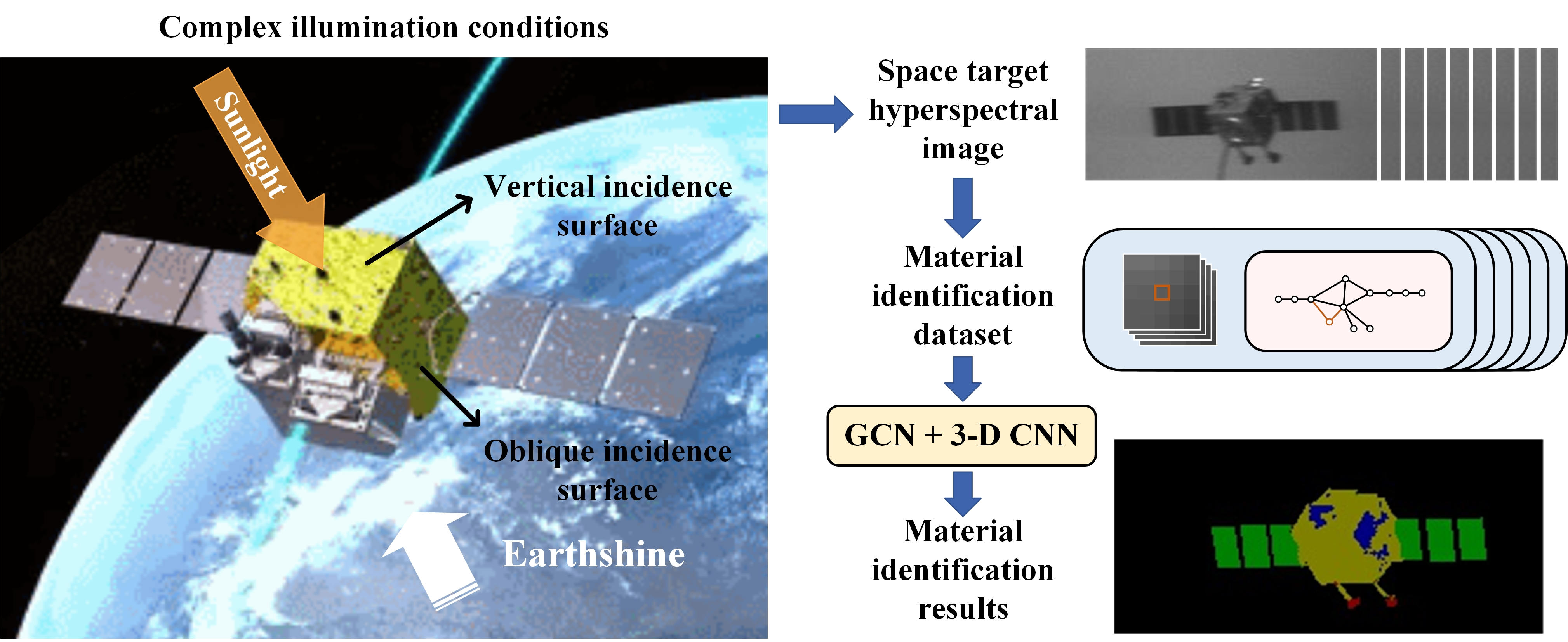
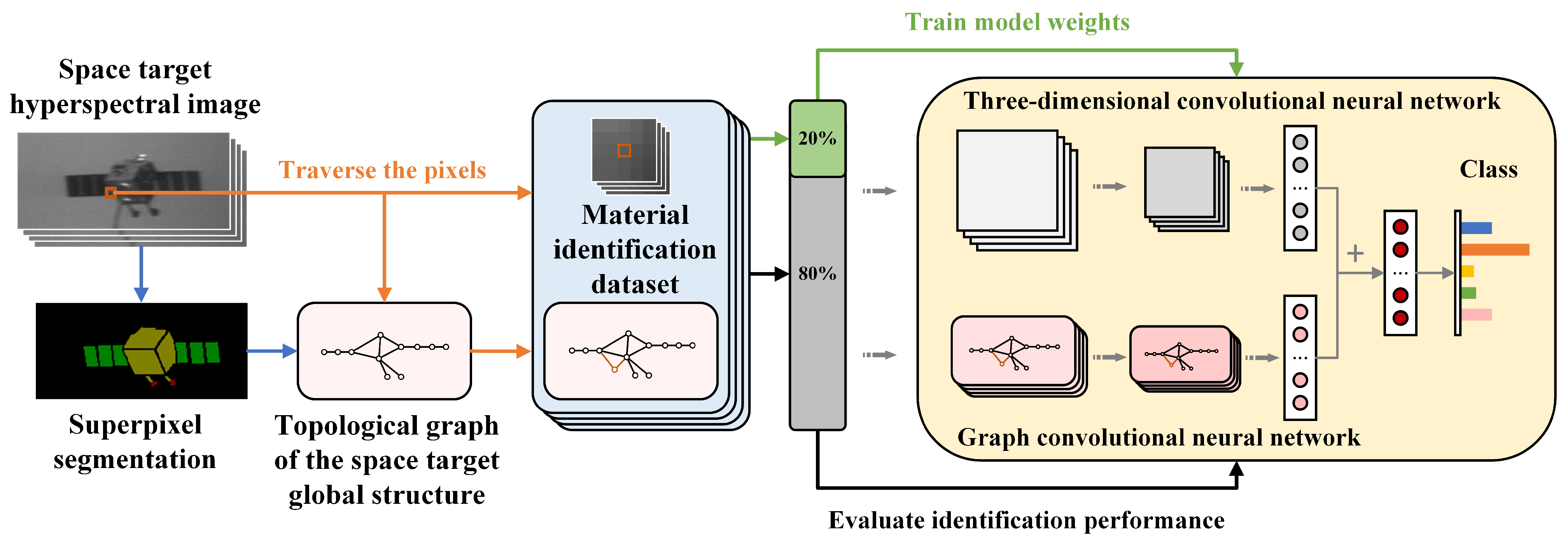
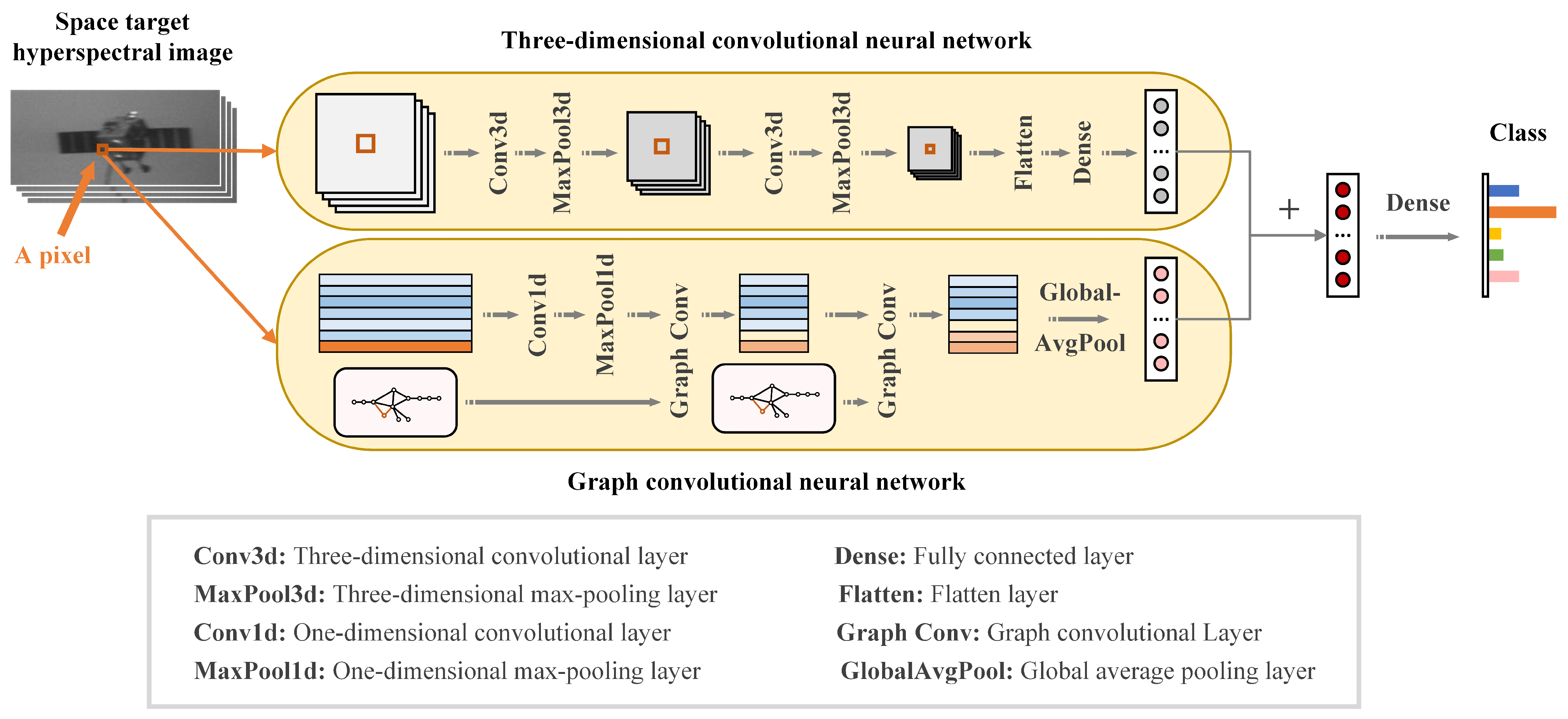
- The graph convolutional neural network (GCN) is introduced to learn the global spatial–spectral features of the space target and combined with a 3-D CNN that can learn local spatial–spectral features. They work together to improve the identification performance under complex illumination conditions.
2. Related Work
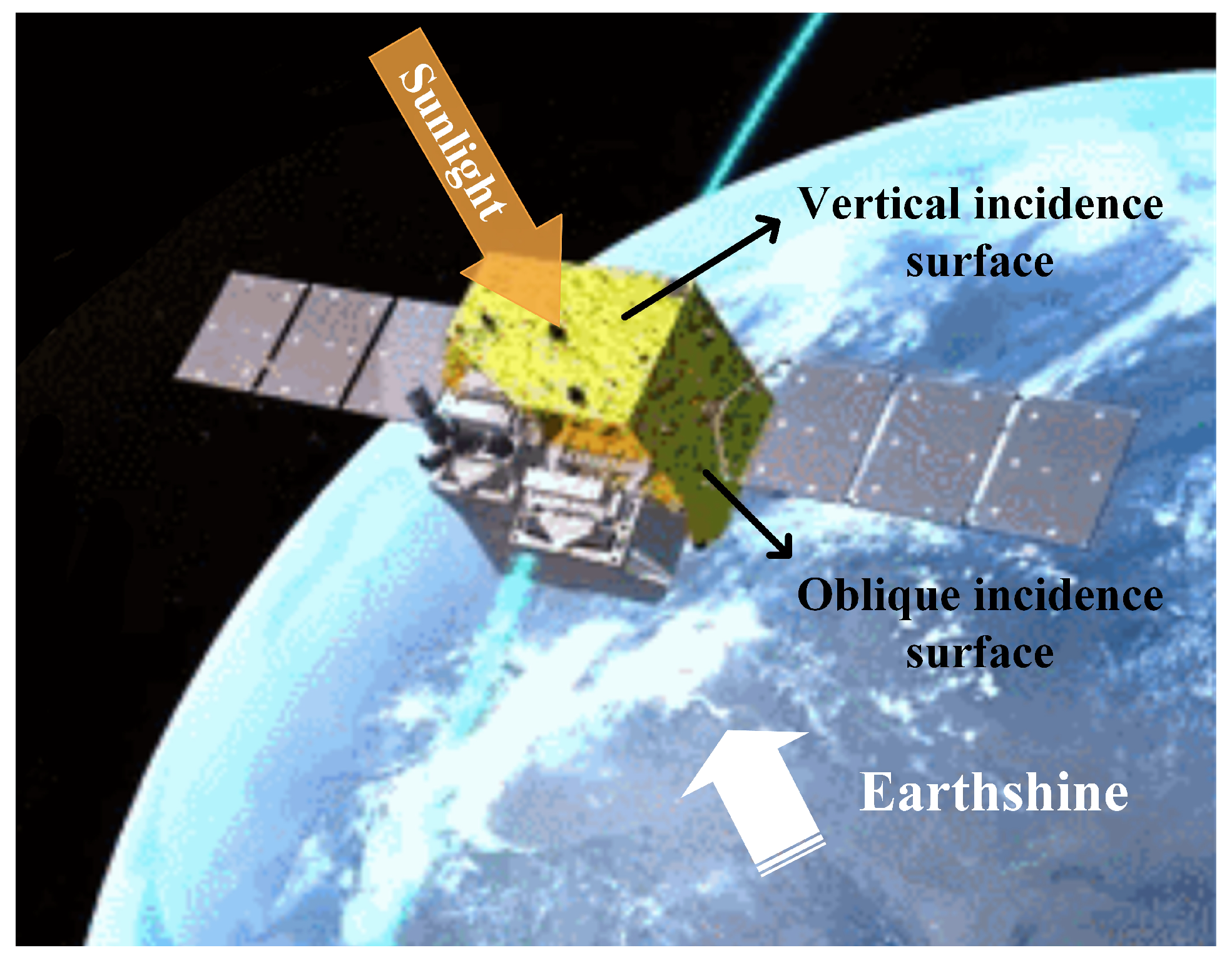
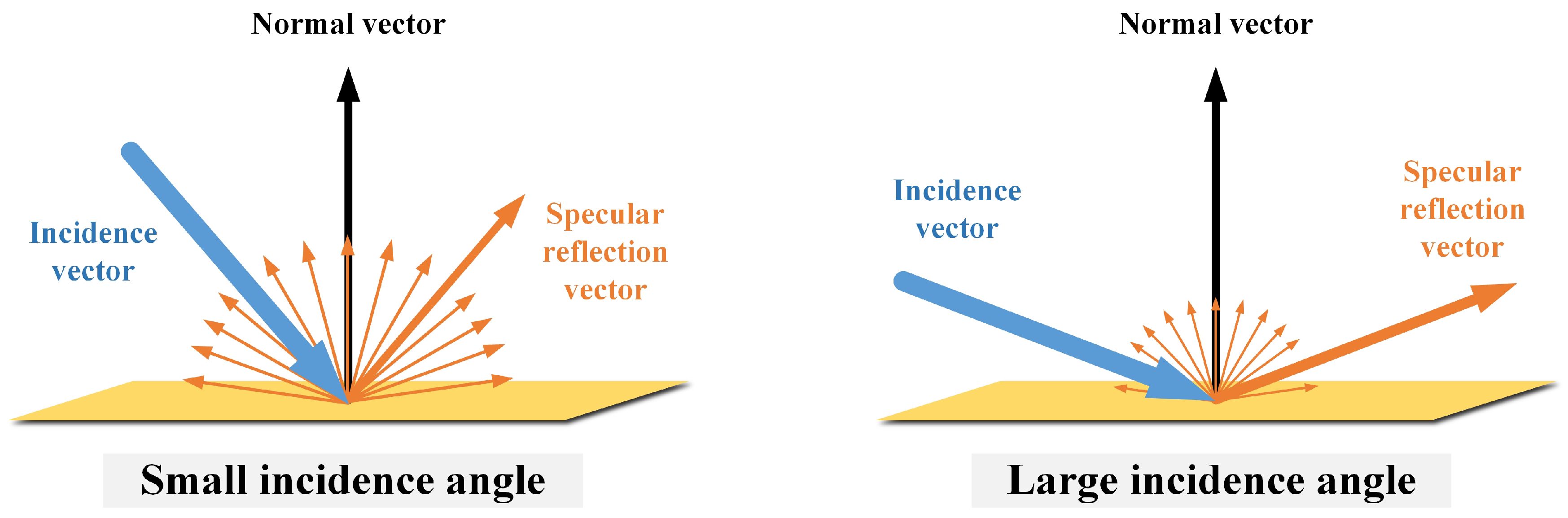
2.1. Complex Illumination Conditions of the Space Target
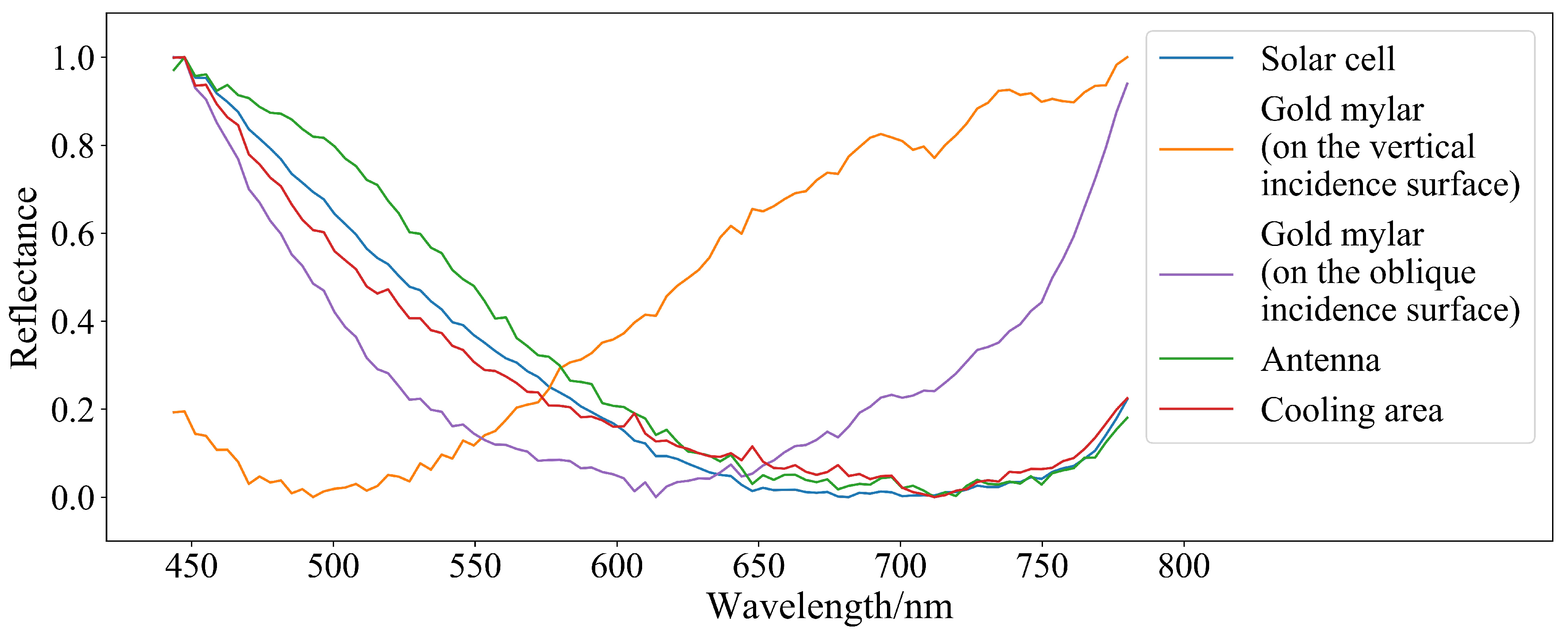
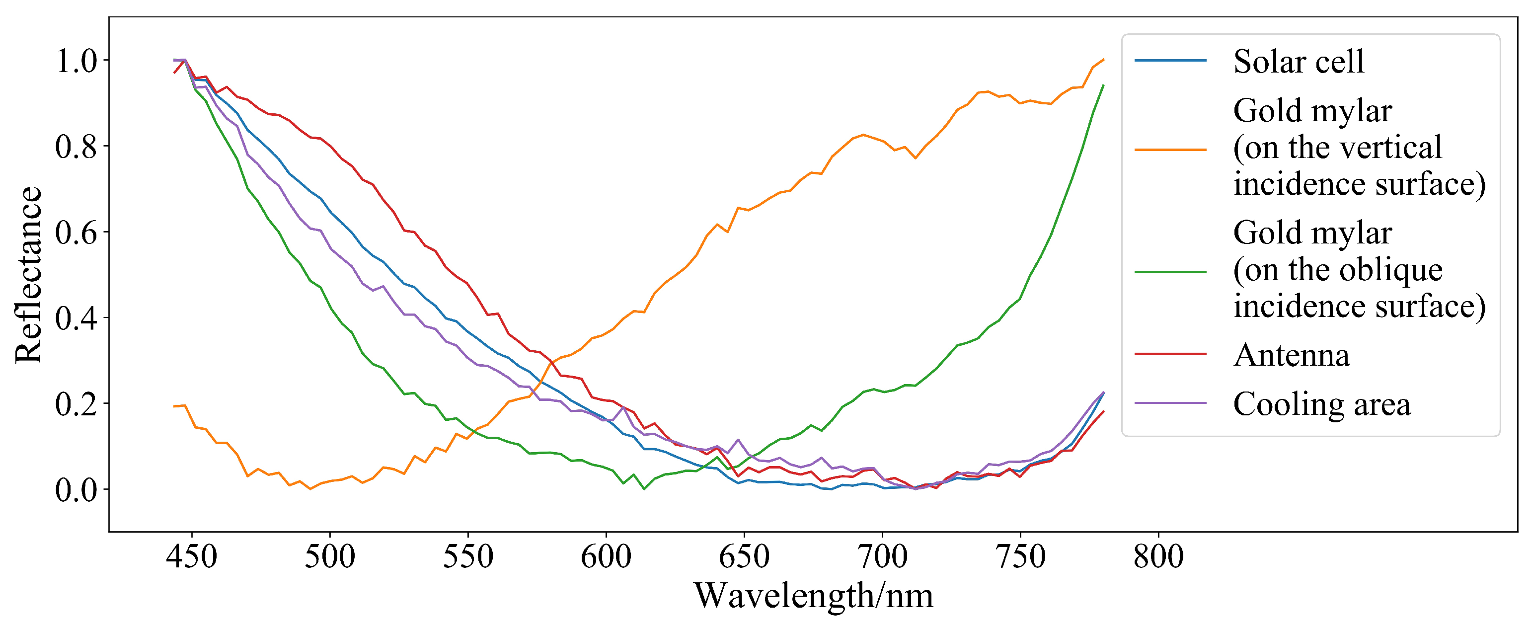
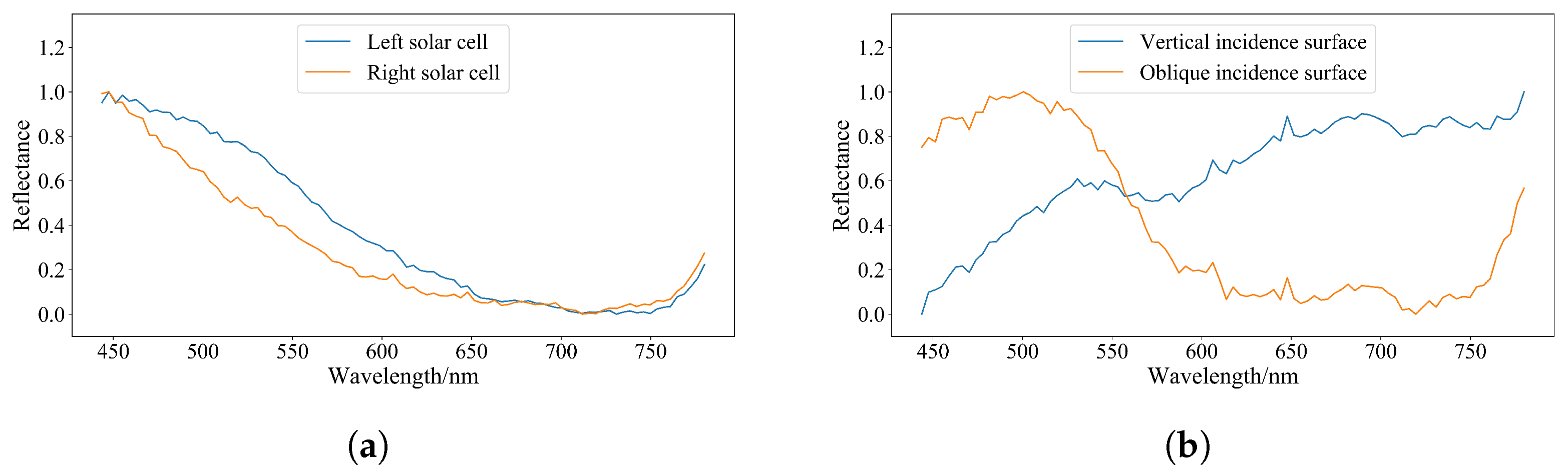
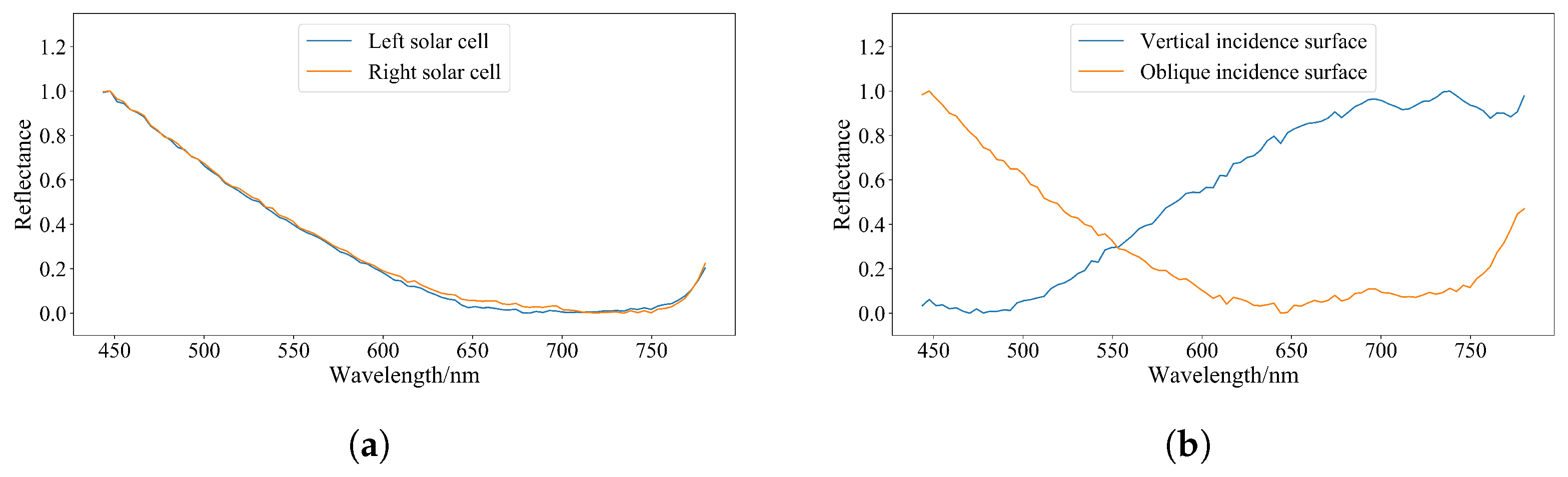
- Under the same illumination conditions, the spectral features of the same material can be very different, i.e., the gold mylar spectra on two surfaces with different orientations shown in Figure 4.
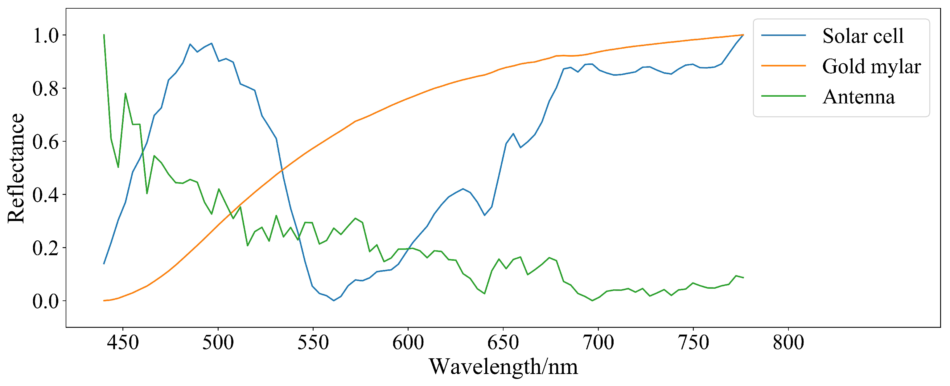
- Under the same illumination conditions, the spectral features of different materials can be very similar, i.e., the spectra of the solar cell, antenna, and cooling area shown in Figure 4.
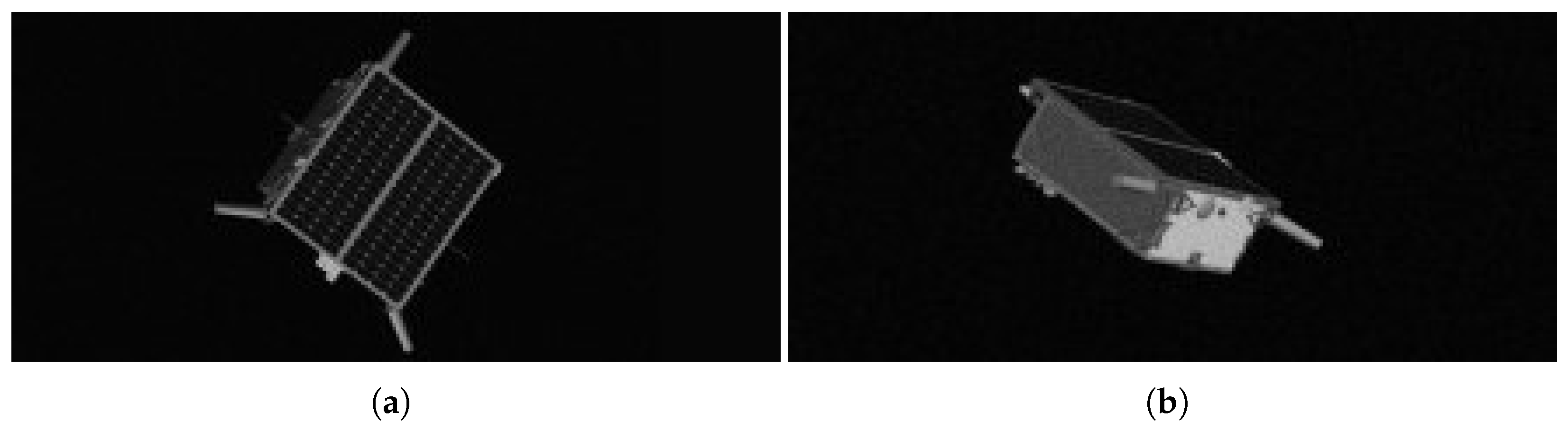
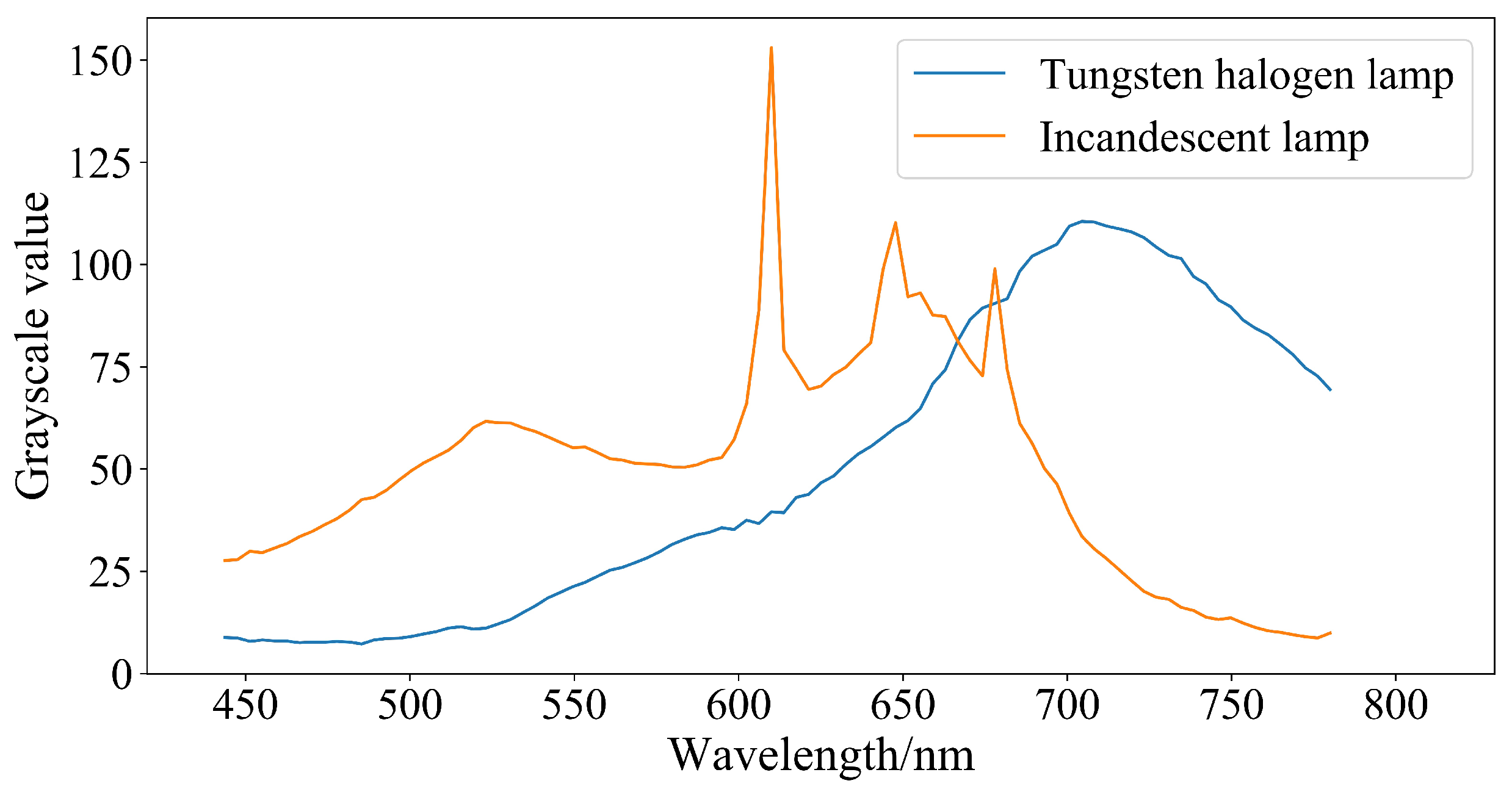
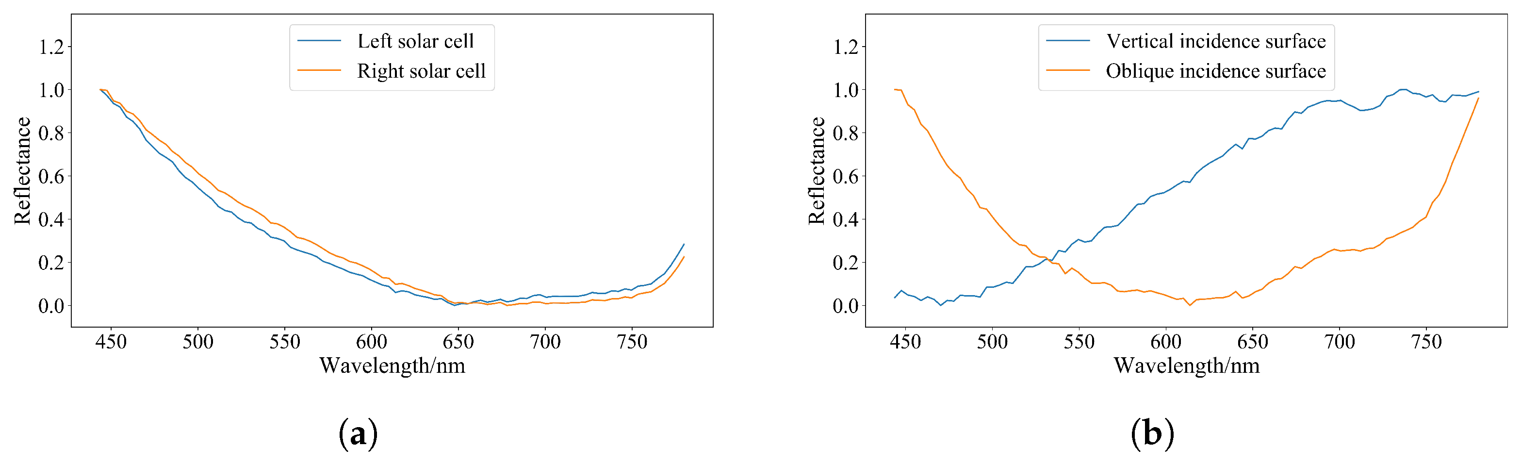
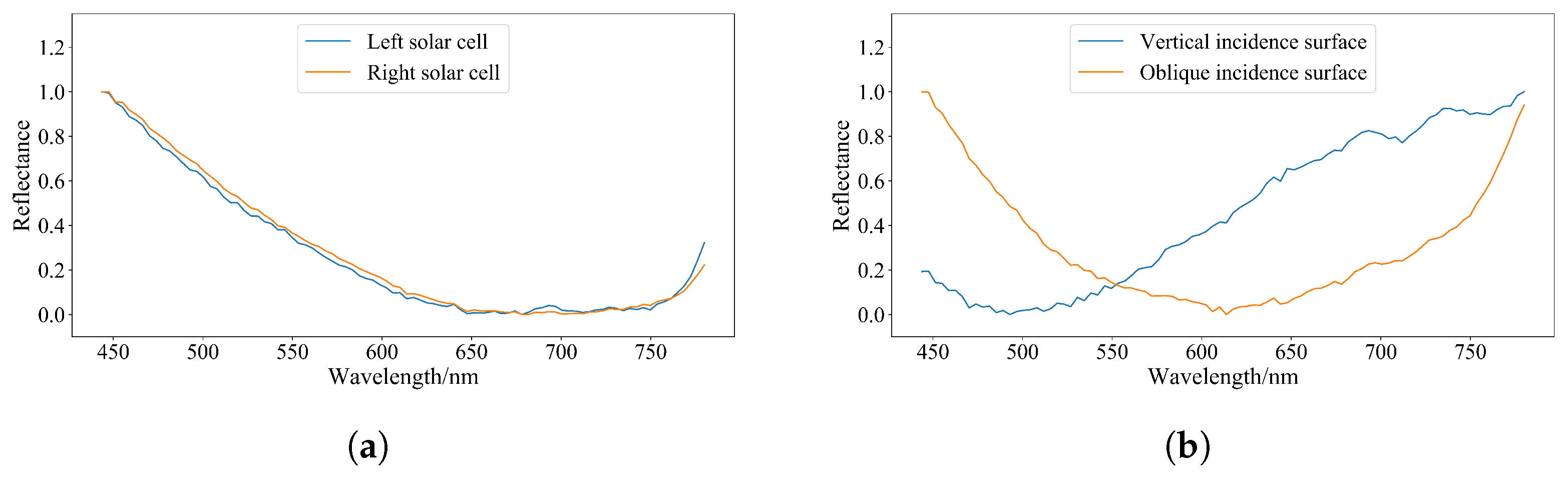
- Under different illumination conditions, the spectral features of the same material can change dramatically, i.e., the gold mylar spectra in the two images shown in Figure 5.
2.2. Graph Convolutional Neural Network
3. Methodology
3.1. The Topological-Graph-Building Method of the Space Target Global Structure
| Algorithm 1 Multiscale, Joint Global-Structure Topological Graph |
Input: (1) Dataset: the hyperspectral image ; (2) Parameters: the initial number of cluster centers and (). Procedure: (2) Build the first global-structure topological graph ; (4) Build the second global-structure topological graph ; (5) Combine and to obtain and ; (6) Connect and , who have overlapping relationship; (7) Build the multiscale, joint global-structure topological graph ; Output: The multiscale, joint global-structure topological graph . |
3.2. Identification Method Based on Fusion of GCN and 3-D CNN
3.3. Data Quality Assessment
4. Results
4.1. Experimental Data
4.1.1. Simulated Data
4.1.2. Measured Data
4.2. Analysis of Identification Results
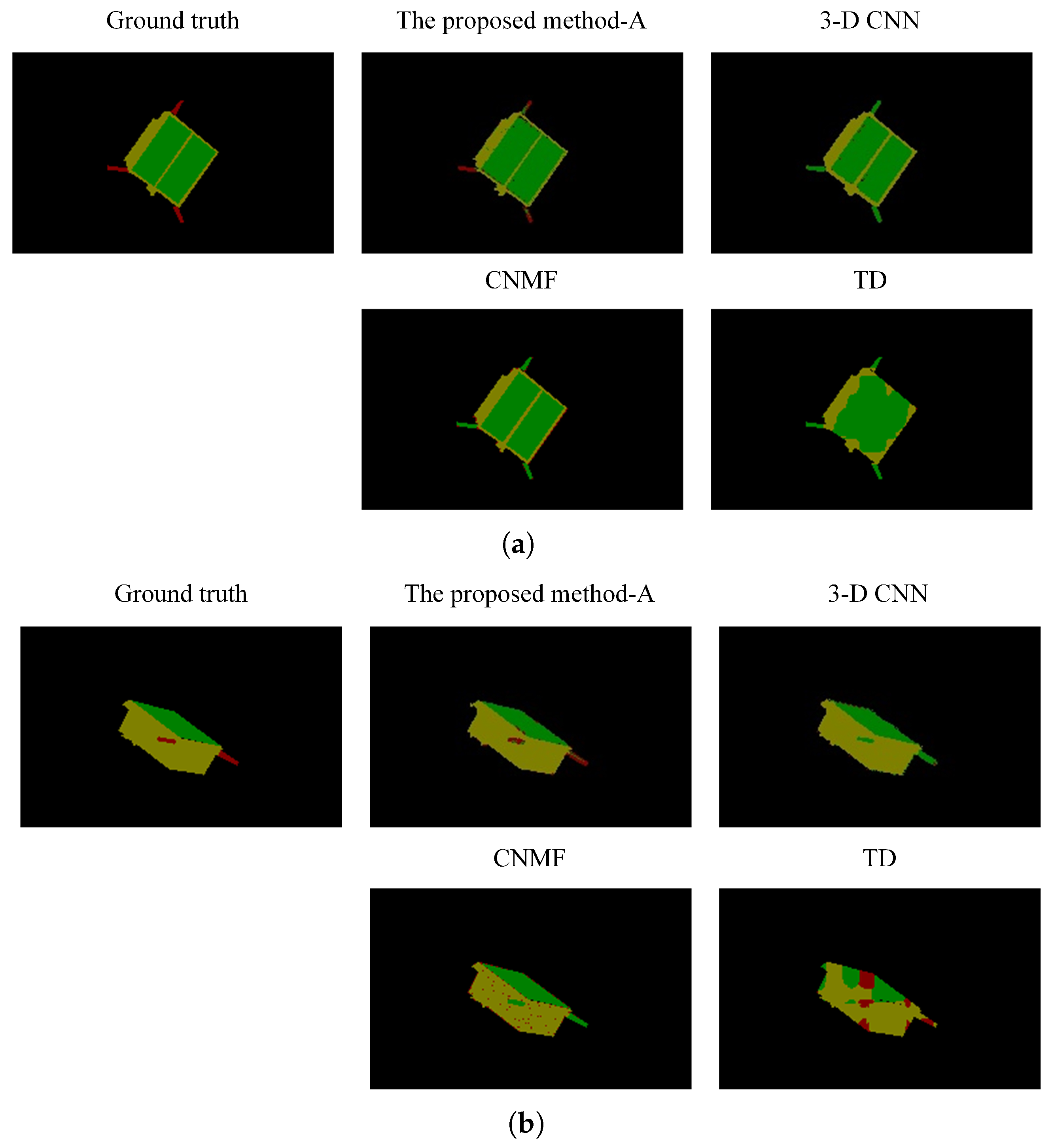
4.2.1. Simulated Data
4.2.2. Measured Data
4.3. Data Quality Assessment Results
5. Discussion
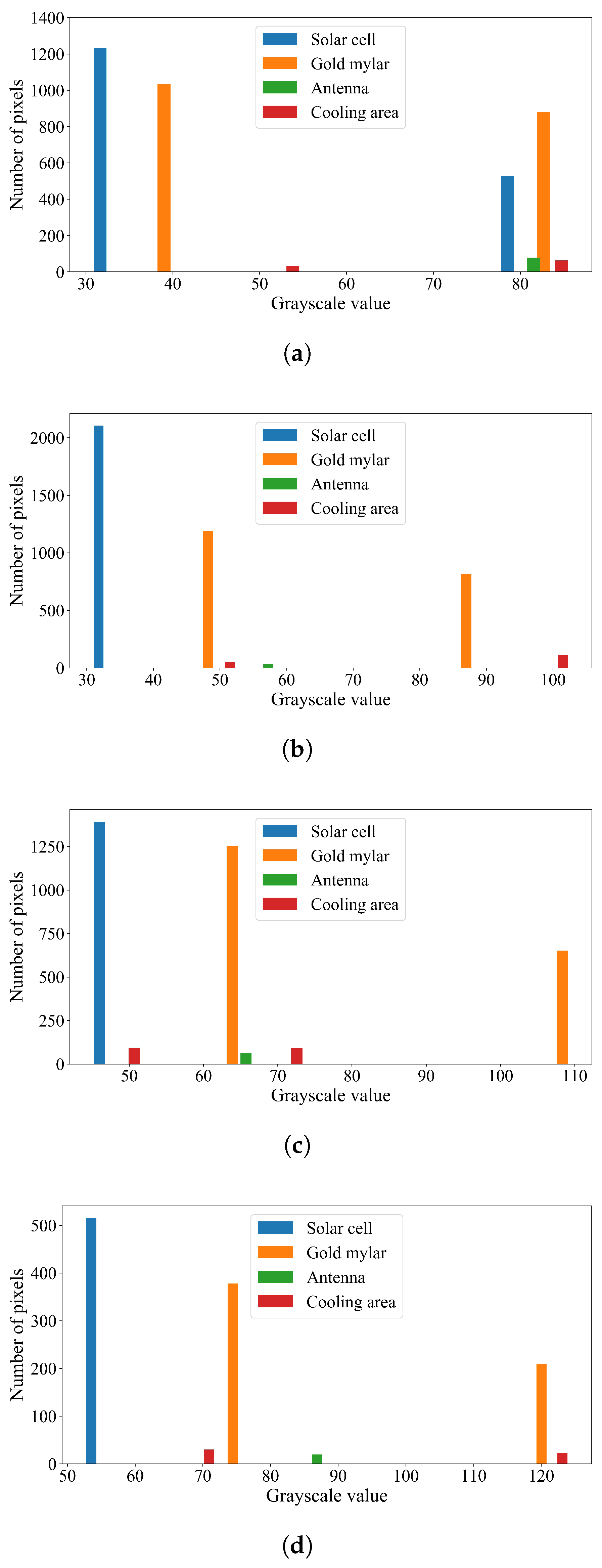
5.1. The Influence Analysis of Illumination Conditions on the Data Distributions
5.2. Comparison of the Results between the Experimental Datasets
5.3. Deficiencies and Improvements under Non-Ideal Imaging Conditions
5.3.1. Image Degradation
5.3.2. Background Distractions
5.3.3. Rapid Changes in Imaging Conditions
6. Conclusions
Author Contributions
Funding
Data Availability Statement
Conflicts of Interest
References
- Mu, J.; Hao, X.; Zhu, W.; Li, S. Review and Prosepect of Intelligent Perception for Non-cooperative Targets. Chin. Space Sci. Technol. 2021, 41, 1–16. [Google Scholar] [CrossRef]
- Deng, S.; Liu, C.; Tan, Y. Research on Spectral Measurement Technology and Surface Material Analysis of Space Target. Spectrosc. Spectr. Anal. 2021, 41, 3299–3306. [Google Scholar] [CrossRef]
- Liu, Y.; Zhao, H.; Zhong, X. The Combined Computational Spectral Imaging Method of Space-based Targets. Spacecr. Recovery Remote Sens. 2021, 42, 74–81. [Google Scholar]
- Abercromby, K.; Okada, J.; Guyote, M.; Hamada, K.; Barker, E. Comparisons of Ground Truth and Remote Spectral Measurements of FORMOSAT and ANDE Spacecraft. In Proceedings of the Advanced Maui Optical and Space Surveillance Technologies Conference, Maui, HI, USA, 12–15 September 2007. [Google Scholar]
- Vananti, A.; Schildknecht, T.; Krag, H. Reflectance spectroscopy characterization of space debris. Adv. Space Res. 2017, 59, 2488–2500. [Google Scholar] [CrossRef] [Green Version]
- Abercromby, K.J.; Rapp, J.; Bedard, D.; Seitzer, P.; Cardona, T.; Cowardin, H.; Barker, E.; Lederer, S. Comparisons of Constrained Least Squares Model Versus Human-in-the-Loop for Spectral Unmixing to Determine Material Type of GEO Debris. In Proceedings of the 6th European Conference on Space Debris, Darmstadt, Germany, 22–25 April 2013; Volume 723, p. 22. [Google Scholar]
- Nie, B.; Yang, L.; Zhao, F.; Zhou, J.; Jing, J. Space Object Material Identification Method of Hyperspectral Imaging Based on Tucker Decomposition. Adv. Space Res. 2021, 67, 2031–2043. [Google Scholar] [CrossRef]
- Velez-Reyes, M.; Yi, J. Hyperspectral Unmixing for Remote Sensing of Unresolved Objects. In Proceedings of the Advanced Maui Optical and Space Surveillance Technologies Conference, Maui, HI, USA, 19–22 September 2023; pp. 573–580. [Google Scholar]
- Yi, J.; Velez-Reyes, M.; Erives, H. Studying the Potential of Hyperspectra Unmixing for Extracting Composition of Unresolved Space Objects using Simulation Models. In Proceedings of the Advanced Maui Optical and Space Surveillance Technologies Conference, Maui, HI, USA, 14–17 September 2021; pp. 603–614. [Google Scholar]
- Li, P.; Li, Z.; Xu, C.; Fang, Y.; Zhang, F. Research on Space Object’s Materials Multi-Color Photometry Identification Based on the Extreme Learning Machine Algorithm. Spectrosc. Spectr. Anal. 2019, 39, 363–369. [Google Scholar]
- Liu, H. The Technology of Spectral Recognition Based on Statistical Machine Learning. Master’s Thesis, Changchun University of Science and Technology, Changchun, China, 2017. [Google Scholar]
- Liu, H.; Li, Z.; Shi, J.; Xin, M.; Cai, H.; Gao, X.; Tan, Y. Study on Classification and Recognition of Materials Based on Convolutinal Neural Network. Laser Infrared 2017, 47, 1024–1028. [Google Scholar]
- Deng, S.; Liu, C.; Tan, Y.; Liu, D.; Zhang, N.; Kang, Z.; Li, Z.; Fan, C.; Jiang, C.; Lu, Z. A Combination of Multiple Deep Learning Methods Applied to Small-Sample Space Objects Classification. Spectrosc. Spectr. Anal. 2022, 42, 609–615. [Google Scholar]
- Gazak, Z.J.; Swindle, R.; McQuaid, I.; Fletcher, J. Exploiting Spatial Information in Raw Spectroscopic Imagery using Convolutional Neural Networks. In Proceedings of the Advanced Maui Optical and Space Surveillance Technologies Conference, Maui, HI, USA, 15–18 September 2020; pp. 395–403. [Google Scholar]
- Vananti, A.; Schildknecht, T.; Krag, H.; Erd, C. Preliminary Results from Reflectance Spectroscopy Observations of Space Debris in GEO. Fifth European Conference on Space Debris. Proc. Esa Spec. Publ. 2009, 672, 41. [Google Scholar]
- Cowardin, H.; Seitzer, P.; Abercromby, K.; Barker, E.; Schildknecht, T. Characterization of Orbital Debris Photometric Properties Derived from Laboratory-Based Measurements. In Proceedings of the Advanced Maui Optical and Space Surveillance Technologies Conference, Maui, HI, USA, 15–18 September 2020; p. 66. [Google Scholar]
- Bédard, D.; Lévesque, M. Analysis of the CanX-1 Engineering Model Spectral Reflectance Measurements. J. Spacecr. Rocket. 2014, 51, 1492–1504. [Google Scholar] [CrossRef]
- Bédard, D.; Wade, G.A.; Abercromby, K. Laboratory Characterization of Homogeneous Spacecraft Materials. J. Spacecr. Rocket. 2015, 52, 1038–1056. [Google Scholar] [CrossRef]
- Sun, C.; Yuan, Y.; Lu, Q. Modeling and Verification of Space-Based Optical Scattering Characteristics of Space Objects. Acta Opt. Sin. 2019, 39, 354–360. [Google Scholar]
- Bédard, D.; Lévesque, M.; Wallace, B. Measurement of the photometric and spectral BRDF of small Canadian satellites in a controlled environment. In Proceedings of the Advanced Maui Optical and Space Surveillance Technologies Conference, Maui, HI, USA, 13–16 September 2011; pp. 1–10. [Google Scholar]
- Bédard, D.; Wade, G.; Monin, D.; Scott, R. Spectrometric characterization of geostationary satellites. In Proceedings of the Advanced Maui Optical and Space Surveillance Technologies Conference, Maui, HI, USA, 11–14 September 2012; pp. 1–11. [Google Scholar]
- Augustine, J.; Eli, Q.; Francis, K. Simultaneous Glint Spectral Signatures of Geosynchronous Satellites from Multiple Telescopes. In Proceedings of the Advanced Maui Optical and Space Surveillance Technologies Conference, Maui, HI, USA, 11–14 September 2018; pp. 1–10. [Google Scholar]
- Perez, M.D.; Musallam, M.A.; Garcia, A.; Ghorbel, E.; Ismaeil, K.A.; Aouada, D.; Henaff, P.L. Detection and Identification of On-Orbit Objects Using Machine Learning. In Proceedings of the 8th European Conference on Space Debris, Darmstadt, Germany, 20–23 April 2021; Volume 8, pp. 1–10. [Google Scholar]
- Chen, Y.; Gao, J.; Zhang, K. R-CNN-Based Satellite Components Detection in Optical Images. Int. J. Aerosp. Eng. 2020, 2020, 8816187. [Google Scholar] [CrossRef]
- Liu, J.; Li, H.; Zhang, Y.; Zhou, J.; Lu, L.; Li, F. Robust Adaptive Relative Position and Attitude Control for Noncooperative Spacecraft Hovering under Coupled Uncertain Dynamics. Math. Probl. Eng. 2019, 2019, 8678473. [Google Scholar] [CrossRef] [Green Version]
- Meftah, M.; Damé, L.; Bolsée, D.; Hauchecorne, A.; Pereira, N.; Sluse, D.; Cessateur, G.; Irbah, A.; Bureau, J.; Weber, M.; et al. SOLAR-ISS: A new reference spectrum based on SOLAR/SOLSPEC observations. Astron. Astrophys. 2018, 2018, 611. [Google Scholar] [CrossRef]
- Guo, X. Study of Spectral Radiation and Scattering Characteristic of Background and Target. Ph.D. Thesis, Xidian University, Xi’an, China, 2018. [Google Scholar]
- Yan, P.; Ma, C.; She, W. Influence of Earth’s Reflective Radiation on Space Target for Space Based Imaging. Acta Phys. Sin. 2015, 64, 1–8. [Google Scholar] [CrossRef]
- Zou, Y.; Zhang, L.; Zhang, J.; Li, B.; Lv, X. Developmental Trends in the Application and Measurement of the Bidirectional Reflection Distribution Function. Sensors 2022, 22, 1739. [Google Scholar] [CrossRef]
- Liu, C.; Li, Z.; Xu, C. A Modified Phong Model for Fresnel Reflection Phenomenon of Commonly Used Materials for Space Targets. Laser Optoelectron. Prog. 2017, 54, 446–454. [Google Scholar]
- Li, J.; Huang, X.; Tu, L. WHU-OHS: A benchmark dataset for large-scale Hersepctral Image classification. Int. J. Appl. Earth Obs. Geoinf. 2022, 113, 103022. [Google Scholar] [CrossRef]
- Li, T.; Zhang, J.; Zhang, Y. Classification of hyperspectral image based on deep belief networks. In Proceedings of the 2014 IEEE International Conference on Image Processing, Paris, France, 27–30 October 2014; pp. 5132–5136. [Google Scholar]
- Mou, L.; Ghamisi, P.; Zhu, X. Deep recurrent neural networks for hyperspectral image classification. IEEE Trans. Geosci. Remote Sens. 2017, 55, 3639–3655. [Google Scholar] [CrossRef] [Green Version]
- Hu, W.; Huang, Y.; Wei, L.; Zhang, F.; Li, H. Deep convolutional neural networks for hyperspectral image classification. J. Sens. 2015, 2015, 258619. [Google Scholar] [CrossRef] [Green Version]
- Li, J.; Du, Q.; Xi, B.; Li, Y. Hyperspectral Image Classification Via Sample Expansion for Convolutional Neural Network. In Proceedings of the 2018 9th Workshop on Hyperspectral Image and Signal Processing: Evolution in Remote Sensing (WHISPERS), Amsterdam, The Netherlands, 23–26 September 2018; pp. 1–5. [Google Scholar] [CrossRef]
- Luo, Y.; Zou, J.; Yao, C.; Zhao, X.; Li, T.; Bai, G. HSI-CNN: A Novel Convolution Neural Network for Hyperspectral Image. In Proceedings of the International Conference on Audio, Language and Image Processing (ICALIP), Shanghai, China, 16–17 July 2018; pp. 464–469. [Google Scholar] [CrossRef] [Green Version]
- Zhu, L.; Chen, Y.; Ghamisi, P.; Benediktsson, J.A. Generative Adversarial Networks for Hyperspectral Image Classification. IEEE Trans. Geosci. Remote Sens. 2018, 56, 5046–5063. [Google Scholar] [CrossRef]
- Chen, Y.; Jiang, H.; Li, C.; Jia, X.; Ghamisi, P. Deep Feature Extraction and Classification of Hyperspectral Images Based on Convolutional Neural Networks. IEEE Trans. Geosci. Remote Sens. 2016, 54, 6232–6251. [Google Scholar] [CrossRef] [Green Version]
- Zou, L.; Zhu, X.; Wu, C.; Liu, Y.; Qu, L. Spectral–Spatial Exploration for Hyperspectral Image Classification via the Fusion of Fully Convolutional Networks. IEEE J. Sel. Top. Appl. Earth Obs. Remote Sens. 2020, 13, 659–674. [Google Scholar] [CrossRef]
- Wang, C.; Bai, X.; Zhou, L.; Zhou, J. Hyperspectral Image Classification Based on Non-Local Neural Networks. In Proceedings of the IGARSS 2019—2019 IEEE International Geoscience and Remote Sensing Symposium, Yokohama, Japan, 28 July–2 August 2019; pp. 584–587. [Google Scholar] [CrossRef]
- Kanthi, M.; Sarma, T.H.; Bindu, C.S. A 3d-Deep CNN Based Feature Extraction and Hyperspectral Image Classification. In Proceedings of the 2020 IEEE India Geoscience and Remote Sensing Symposium (InGARSS), Virtual, 2–4 December 2020; pp. 229–232. [Google Scholar] [CrossRef]
- Zhang, H.; Chen, Y.; He, X.; Shen, X. Boosting CNN for Hyperspectral Image Classification. In Proceedings of the 2021 IEEE International Geoscience and Remote Sensing Symposium IGARSS, Brussels, Belgium, 11–16 July 2021; pp. 3673–3676. [Google Scholar] [CrossRef]
- Xu, Z.; Yu, H.; Zheng, K.; Gao, L.; Song, M. A Novel Classification Framework for Hyperspectral Image Classification Based on Multiscale Spectral-Spatial Convolutional Network. In Proceedings of the 2021 11th Workshop on Hyperspectral Imaging and Signal Processing: Evolution in Remote Sensing (WHISPERS), Amsterdam, The Netherlands, 24–26 March 2021; pp. 1–5. [Google Scholar] [CrossRef]
- Feng, J.; Wu, X.; Shang, R.; Sui, C.; Li, J.; Jiao, L.; Zhang, X. Attention multibranch convolutional neural network for hyperspectral image classification based on adaptive region search. IEEE Trans. Geosci. Remote Sens. 2021, 59, 5054–5070. [Google Scholar] [CrossRef]
- Kipf, T.; Welling, M. Semi-Supervised Classification with Graph Convolutional Networks. In Proceedings of the International Conference of Legal Regulators (ICLR), Singapore, 5–6 October 2017. [Google Scholar]
- Qin, A.; Shang, Z.; Tian, J.; Wang, Y.; Zhang, T.; Tang, Y.Y. Spectral–Spatial Graph Convolutional Networks for Semisupervised Hyperspectral Image Classification. IEEE Geosci. Remote Sens. Lett. 2019, 16, 241–245. [Google Scholar] [CrossRef]
- Wan, S.; Gong, C.; Zhong, P.; Pan, S.; Li, G.; Yang, J. Hyperspectral image classification with context-aware dynamic graph convolutional network. IEEE Trans. Geosci. Remote Sens. 2021, 59, 597–612. [Google Scholar] [CrossRef]
- Wan, S.; Gong, C.; Zhong, P.; Du, B.; Zhang, L.; Yang, J. Multiscale Dynamic Graph Convolutional Network for Hyperspectral Image Classification. IEEE Trans. Geosci. Remote Sens. 2020, 58, 3162–3177. [Google Scholar] [CrossRef] [Green Version]
- Hong, D.; Gao, L.; Yao, J.; Zhang, B.; Plaza, A.; Chanussot, J. Graph Convolutional Networks for Hyperspectral Image Classification. IEEE Trans. Geosci. Remote Sens. 2021, 59, 5966–5978. [Google Scholar] [CrossRef]
- Zhang, M.; Luo, H.; Song, W.; Mei, H.; Su, C. Spectral-Spatial Offset Graph Convolutional Networks for Hyperspectral Image Classification. Remote Sens. 2021, 13, 4342. [Google Scholar] [CrossRef]
- Ding, Y.; Zhang, Z.; Zhao, X.; Hong, D.; Cai, W.; Yu, C.; Yang, N.; Cai, W. Multi-feature fusion: Graph neural network and CNN combining for hyperspectral image classification. Neurocomputing 2022, 501, 246–257. [Google Scholar] [CrossRef]
- Ding, Y.; Zang, Z.; Zhao, X.; Cai, W.; He, F.; Cai, Y.; Cai, W.W. Deep hybrid: Multi-graph neural network collaboration for hyperspectral image classification. Def. Technol. 2022. [Google Scholar] [CrossRef]
- Zhang, Z.; Ding, Y.; Zhao, X.; Siye, L.; Yang, N.; Cai, Y.; Zhan, Y. Multireceptive field: An adaptive path aggregation graph neural framework for hyperspectral image classification. Expert Syst. Appl. 2023, 217, 119508. [Google Scholar] [CrossRef]
- Ding, Y.; Zhang, Z.; Zhao, X.; Cai, W.; Yang, N.; Hu, H.; Huang, X.; Cao, Y.; Cai, W. Unsupervised Self-Correlated Learning Smoothy Enhanced Locality Preserving Graph Convolution Embedding Clustering for Hyperspectral Images. IEEE Trans. Geosci. Remote Sens. 2022, 60, 5536716. [Google Scholar] [CrossRef]
- Ding, Y.; Zhang, Z.; Zhao, X.; Cai, Y.; Li, S.; Deng, B.; Cai, W. Self-Supervised Locality Preserving Low-Pass Graph Convolutional Embedding for Large-Scale Hyperspectral Image Clustering. IEEE Trans. Geosci. Remote Sens. 2022, 60, 5536016. [Google Scholar] [CrossRef]
- Ding, Y.; Zhao, X.; Zhang, Z.; Cai, W.; Yang, N.; Zhan, Y. Semi-Supervised Locality Preserving Dense Graph Neural Network with ARMA Filters and Context-Aware Learning for Hyperspectral Image Classification. IEEE Trans. Geosci. Remote Sens. 2022, 60, 5511812. [Google Scholar] [CrossRef]
- Achanta, R.; Shaji, A.; Smith, K.; Lucchi, A.; Fua, P.; Süsstrunk, S. SLIC superpixels compared to state-of-the-art superpixel methods. IEEE Trans. Pattern Anal. Mach. Intell. 2012, 34, 2274–2282. [Google Scholar] [CrossRef] [Green Version]
- Smith, L.N. Cyclical Learning Rates for Training Neural Networks. In Proceedings of the 2017 IEEE Winter Conference on Applications of Computer Vision (WACV), Waikoloa, HI, USA, 3–7 January 2017; pp. 464–472. [Google Scholar] [CrossRef] [Green Version]
- Prechelt, L. Early Stopping—But When? In Neural Networks: Tricks of the Trade, Lecture Notes in Computer Science; Springer: Berlin/Heidelberg, Germany, 2012; Volume 7700. [Google Scholar] [CrossRef]
- Sammut, C.; Webb, G.I. F1-Measure. In Encyclopedia of Machine Learning and Data Mining; Springer: Boston, MA, USA, 2017; p. 16. [Google Scholar] [CrossRef]
- Thompson, W.; Walter, S. A reappraisal of the kappa coefficient. J. Clin. Epidemiol. 1988, 41, 949–958. [Google Scholar] [CrossRef]
- Xu, Z.; Zhao, H.; Jia, G. Influence of The AOTF Rear Cut Angle on Spectral Image Quality. Infrared Laser Eng. 2022, 51, 373–379. [Google Scholar]
- Chen, X.; Wan, M.; Xu, Y.; Qian, W.; Chen, Q.; Gu, G. Infrared Remote Sensing Imaging Simulation Method for Earth’s Limb Scene. Infrared Laser Eng. 2022, 51, 24–31. [Google Scholar]
- Xie, J.; Xiang, J.; Chen, J.; Hou, X.; Zhao, X.; Shen, L. C2 AM: Contrastive learning of Class-agnostic Activation Map for Weakly Supervised Object Localization and Semantic Segmentation. In Proceedings of the 2022 IEEE/CVF Conference on Computer Vision and Pattern Recognition (CVPR), New Orleans, LA, USA, 18–24 June 2022; pp. 979–988. [Google Scholar] [CrossRef]
- Borelli, G.; Gaias, G.; Colombo, C. Rendezvous and Proximity Operations Design of An Active Debris Removal Service to A Large Constellation Fleet. Acta Astronaut. 2023, 205, 33–46. [Google Scholar] [CrossRef]
- Zhang, R.; Han, C.; Rao, Y.I.; Yin, J. Spacecraft Fast Fly-Around Formations Design Using the Bi-Teardrop Configuration. J. Guid. Control. Dyn. 2018, 41, 1542–1555. [Google Scholar] [CrossRef]
- Li, Y.; Wang, B.; Liu, C. Long-term Accompanying Flight Control of Satellites with Low Fuel Consumption. In Proceedings of the 2016 Chinese Control and Decision Conference (CCDC), Yinchuan, China, 28–30 May 2016; pp. 360–363. [Google Scholar] [CrossRef]
- Dwivedi, V.P.; Rampášek, L.; Galkin, M.; Parviz, A.; Wolf, G.; Luu, A.; Beaini, D. Long Range Graph Benchmark. arXiv 2022, arXiv:2206.08164. [Google Scholar]


| T0 | T1 | T2 | T3 | |
|---|---|---|---|---|
| Illumination conditions | 10:1 | 10:1 | 20:3 | 10:1 |
| Spatial resolution (cm/pixel) | 3.2 | 3.2 | 3.2 | 6.4 |
| Steps | Dimensions and Parameters | |
|---|---|---|
| Simulated Data | Measured Data | |
|
| |
| Inputs |
|
|
|
| |
| SLIC |
|
|
|
| |
| The Network |
| |
| ||
| ||
| ||
| ||
| ||
|
| |
| Output |
|
|
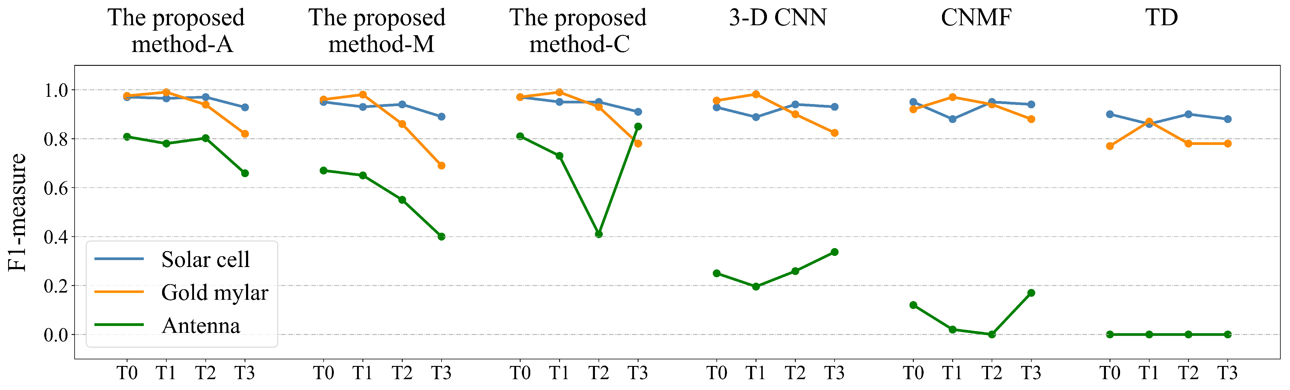
| Class | The Proposed Method | |||||||||||
|---|---|---|---|---|---|---|---|---|---|---|---|---|
| -A | -M | -C | ||||||||||
| T0 | T1 | T2 | T3 | T0 | T1 | T2 | T3 | T0 | T1 | T2 | T3 | |
| Solar cell | 97 | 96 | 97 | 93 | 95 | 93 | 94 | 89 | 97 | 95 | 95 | 91 |
| Gold mylar | 97 | 99 | 94 | 82 | 96 | 98 | 86 | 69 | 97 | 99 | 93 | 78 |
| Antenna | 81 | 78 | 80 | 66 | 67 | 65 | 55 | 40 | 81 | 73 | 41 | 85 |
| Class | 3-D CNN | CNMF | TD | |||||||||
| T0 | T1 | T2 | T3 | T0 | T1 | T2 | T3 | T0 | T1 | T2 | T3 | |
| Solar cell | 93 | 89 | 94 | 93 | 95 | 88 | 95 | 94 | 90 | 86 | 90 | 88 |
| Gold mylar | 96 | 98 | 90 | 82 | 92 | 97 | 94 | 88 | 77 | 87 | 78 | 78 |
| Antenna | 25 | 20 | 26 | 34 | 12 | 2 | 0 | 17 | 0 | 0 | 0 | 0 |
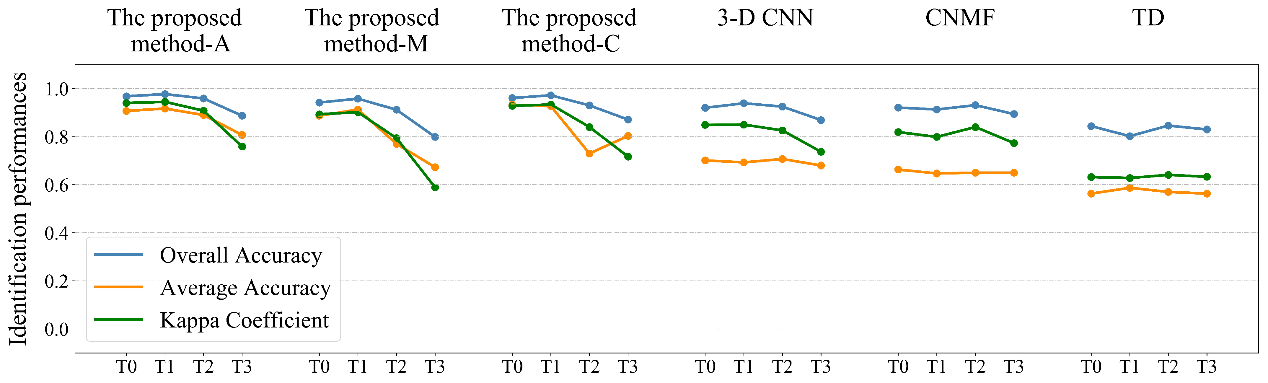
| Method | OA(%) | AA(%) | Kappa | ||||||||||
|---|---|---|---|---|---|---|---|---|---|---|---|---|---|
| T0 | T1 | T2 | T3 | T0 | T1 | T2 | T3 | T0 | T1 | T2 | T3 | ||
| The | -A | 96.8 | 97.7 | 95.9 | 88.7 | 90.7 | 91.7 | 89.0 | 80.7 | 0.940 | 0.945 | 0.908 | 0.759 |
| proposed | -M | 94.2 | 95.8 | 91.2 | 79.9 | 88.7 | 91.3 | 77.0 | 67.3 | 0.893 | 0.902 | 0.794 | 0.589 |
| method | -C | 96.1 | 97.2 | 93.0 | 87.1 | 93.3 | 92.7 | 73.0 | 80.3 | 0.928 | 0.934 | 0.840 | 0.717 |
| 3-D CNN | 92.0 | 93.9 | 92.5 | 86.9 | 70.1 | 69.3 | 70.7 | 68.0 | 0.849 | 0.850 | 0.826 | 0.737 | |
| CNMF | 92.1 | 91.3 | 93.1 | 89.4 | 66.3 | 64.7 | 65.0 | 65.0 | 0.819 | 0.799 | 0.840 | 0.773 | |
| TD | 84.4 | 80.2 | 84.6 | 83.0 | 56.3 | 58.7 | 57.0 | 56.3 | 0.632 | 0.628 | 0.641 | 0.633 | |
| T0 | T1 | T2 | T3 | |
|---|---|---|---|---|
| Illumination conditions | + Y-axis; − Z-axis | − Z-axis | − X-axis | + Y-axis |
| Spatial resolution (cm/pixel) | 5.4 | 5.4 | 5.4 | 10.8 |
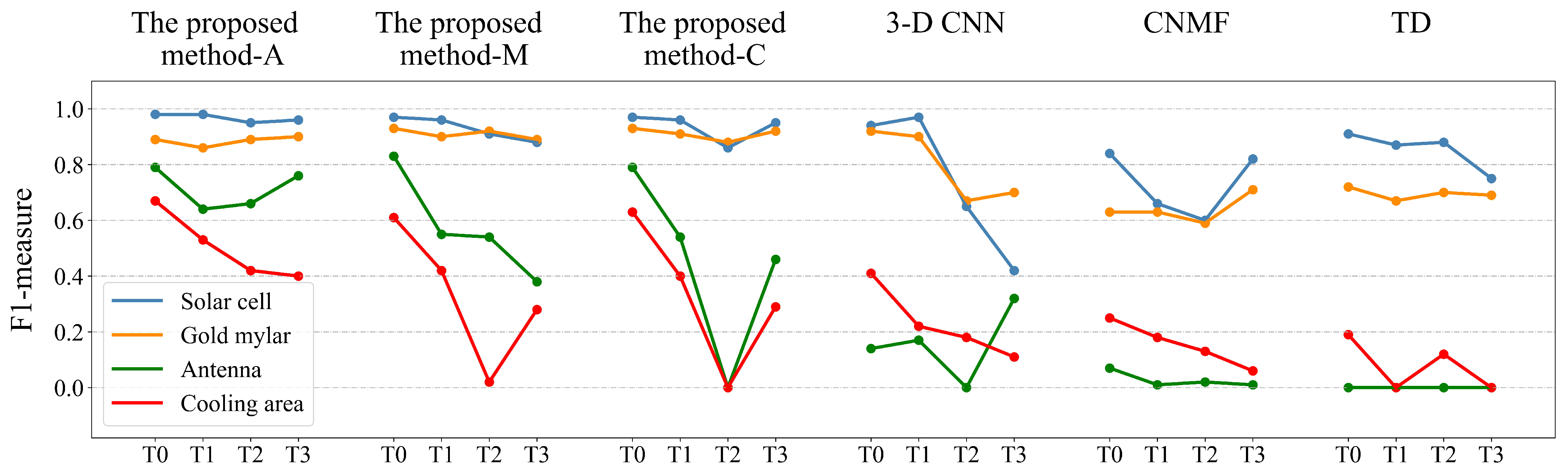
| Class | The Proposed Method | |||||||||||
|---|---|---|---|---|---|---|---|---|---|---|---|---|
| -A | -M | -C | ||||||||||
| T0 | T1 | T2 | T3 | T0 | T1 | T2 | T3 | T0 | T1 | T2 | T3 | |
| Solar cell | 98 | 98 | 95 | 96 | 97 | 96 | 91 | 88 | 97 | 96 | 86 | 95 |
| Gold mylar | 89 | 86 | 89 | 90 | 93 | 90 | 92 | 89 | 93 | 91 | 88 | 92 |
| Antenna | 79 | 64 | 66 | 76 | 83 | 55 | 54 | 38 | 79 | 57 | 0 | 46 |
| Cooling area | 67 | 53 | 42 | 40 | 61 | 42 | 2 | 28 | 63 | 40 | 0 | 29 |
| Class | 3-D CNN | CNMF | TD | |||||||||
| T0 | T1 | T2 | T3 | T0 | T1 | T2 | T3 | T0 | T1 | T2 | T3 | |
| Solar cell | 94 | 97 | 65 | 42 | 84 | 66 | 60 | 82 | 91 | 87 | 88 | 75 |
| Gold mylar | 92 | 90 | 67 | 70 | 63 | 63 | 59 | 71 | 72 | 67 | 70 | 69 |
| Antenna | 14 | 17 | 0 | 32 | 7 | 1 | 2 | 1 | 0 | 0 | 0 | 0 |
| Cooling area | 41 | 22 | 18 | 11 | 25 | 18 | 13 | 6 | 19 | 0 | 12 | 0 |
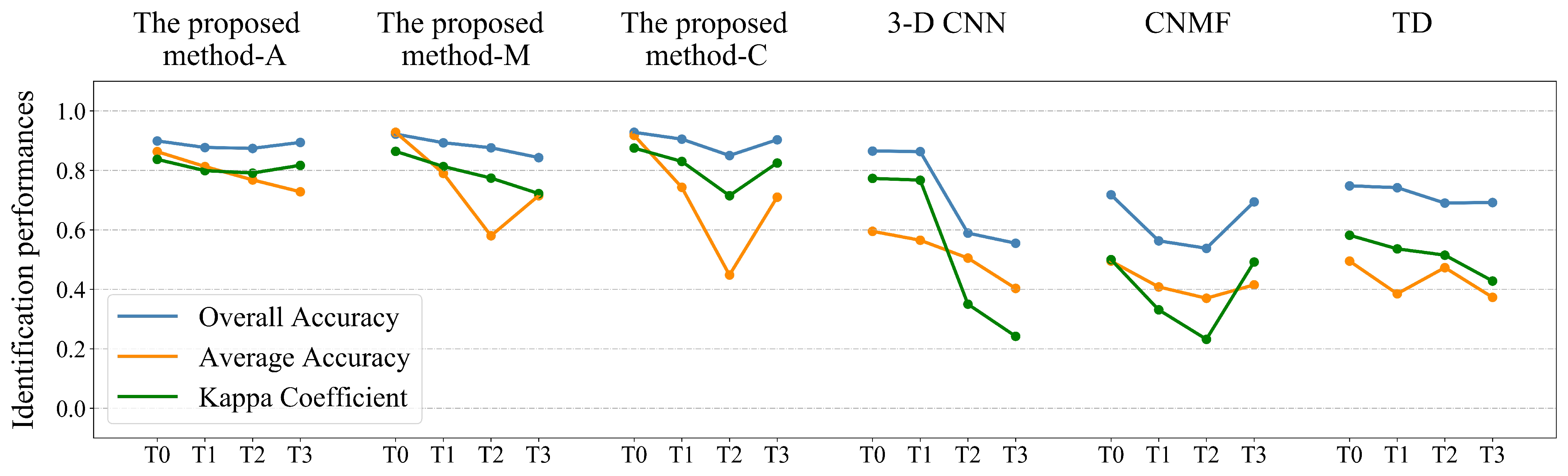
| Method | OA(%) | AA(%) | Kappa | ||||||||||
|---|---|---|---|---|---|---|---|---|---|---|---|---|---|
| T0 | T1 | T2 | T3 | T0 | T1 | T2 | T3 | T0 | T1 | T2 | T3 | ||
| The | -A | 89.9 | 87.7 | 87.4 | 89.4 | 86.3 | 81.3 | 76.8 | 72.8 | 0.837 | 0.799 | 0.791 | 0.817 |
| proposed | -M | 92.2 | 89.3 | 87.6 | 84.3 | 92.8 | 79.0 | 58.0 | 71.5 | 0.864 | 0.813 | 0.774 | 0.722 |
| method | -C | 92.8 | 90.5 | 85.0 | 90.3 | 91.8 | 74.3 | 44.8 | 71.0 | 0.875 | 0.830 | 0.715 | 0.825 |
| 3-D CNN | 86.5 | 86.3 | 58.9 | 55.5 | 59.5 | 56.5 | 50.5 | 40.3 | 0.773 | 0.767 | 0.350 | 0.242 | |
| CNMF | 71.8 | 56.3 | 53.8 | 69.4 | 49.5 | 40.8 | 37.0 | 41.5 | 0.500 | 0.331 | 0.232 | 0.492 | |
| TD | 74.8 | 74.2 | 69.0 | 69.2 | 49.5 | 38.5 | 47.3 | 37.3 | 0.582 | 0.536 | 0.515 | 0.428 | |
| Simulated data | 7.7473 | 1.6508 | 4.6930 |
| Measured data | 0.7777 | 2.4307 | 0.3199 |
Disclaimer/Publisher’s Note: The statements, opinions and data contained in all publications are solely those of the individual author(s) and contributor(s) and not of MDPI and/or the editor(s). MDPI and/or the editor(s) disclaim responsibility for any injury to people or property resulting from any ideas, methods, instructions or products referred to in the content. |
© 2023 by the authors. Licensee MDPI, Basel, Switzerland. This article is an open access article distributed under the terms and conditions of the Creative Commons Attribution (CC BY) license (https://creativecommons.org/licenses/by/4.0/).
Share and Cite
Li, N.; Gong, C.; Zhao, H.; Ma, Y. Space Target Material Identification Based on Graph Convolutional Neural Network. Remote Sens. 2023, 15, 1937. https://doi.org/10.3390/rs15071937
Li N, Gong C, Zhao H, Ma Y. Space Target Material Identification Based on Graph Convolutional Neural Network. Remote Sensing. 2023; 15(7):1937. https://doi.org/10.3390/rs15071937
Chicago/Turabian StyleLi, Na, Chengeng Gong, Huijie Zhao, and Yun Ma. 2023. "Space Target Material Identification Based on Graph Convolutional Neural Network" Remote Sensing 15, no. 7: 1937. https://doi.org/10.3390/rs15071937