Inversion of Wind and Temperature from Low SNR FPI Interferograms

Abstract

The temperature and wind in the middle and upper atmosphere can be obtained by recording the Doppler shift and broadening of the airglow emission, which is reflected by the interference ring from a ground-based Fabry–Perot interferometer (FPI) system. FPI observations are highly susceptible to weather and the external environment, which seriously affect the signal-to-noise ratio (SNR) of FPI interferograms. An SNR can significantly increase errors in determining the center of the interferogram, leading to inaccurate wind and temperature inversions. The calculation shows that the wind inversion from the interferogram decreases and the temperature increases for larger central errors. In this paper, we propose the maximum standard deviation method (MSDM) with high accuracy and robustness to determine the interference ring center. The performance of the MSDM is better achieved by using more than 100 1D interferogram bins to determine the center of interferograms. The robustness of the MSDM is investigated by computing numerous simulated interferograms with white Gaussian noise and Poisson noise, and compared with the two algorithms of binarization and peak fitting, which are usually used to invert wind and temperature from the interference ring of FPI. The results show that MSDM has higher accuracy and robustness than the other two algorithms. We also simulate the distortion interferogram when the FPI may be illuminated by inhomogeneous background light, which can introduce additional errors in wind and temperature, and the MSDM still performs better. Finally, we invert the wind and temperature from the real airglow interferogram by the Kelan (38.7°N, 111.6°E) FPI, which shows that both the wind and temperature inverted by MSDM better agree well with the FPI product than the other two algorithms. Therefore, the MSDM helps to improve the accuracy and stability to invert the wind and temperature.

1. Introduction

Temperature and wind are key parameters for characterizing the extremely complex dynamic and thermodynamic changes and properties in the middle and upper atmosphere. The wind is an important player in the spatial transport of energy and momentum in the atmosphere. Atmospheric temperature is mainly influenced by solar radiation and atmospheric wave transmission. There are many instruments to detect atmospheric winds and temperatures at different altitudes, such as satellites, meteor radars, and lidars. However, the FPI is the only ground-based device that can detect thermospheric winds and temperatures at 250 km. Studying winds and temperatures helps to understand the environmental properties of the middle and upper atmosphere and promotes the study of atmospheric wave and energy coupling [1]. There are a large number of studies using FPI to study atmospheric mechanisms [2,3,4,5]. Liu et al. [6] studied planetary wave-type oscillations using the Xinglong and Millstone Mountain FPIs and found that planetary wave-type oscillations occur more often from May to October with annual and semiannual variations. Liu et al. [7] investigated the response of nighttime thermospheric temperature multi-day oscillations to solar and geomagnetic activity using FPI data.

The FPI can detect the atmospheric wind and temperature because it has a very high accuracy to resolve the Doppler shift of airglow by the wind and the Doppler broadening by the temperature. The airglow, widely present in the atmosphere, is the product mainly of chemical reactions in the upper atmosphere, which is studied by many researchers [8,9,10]. The temporal and spatial distribution of airglow is modulated by a variety of atmospheric dynamical processes and space environments such as tides, planetary waves, and solar activity. Therefore, airglow is a good tracer of atmospheric photochemical and dynamical processes. FPI is used to estimate the atmospheric wind speed and temperature by observing the airglow. Currently, the existing FPI receives three wavelengths, namely OH 892.0 nm at 87 km, OI 557.7 nm at 97 km, and OI 630.0 nm at 250 km [11,12,13,14].

The FPI is equipped with a high-precision etalon to resolve the Doppler shift and Doppler broadening of the airglow. The convolution of the airglow emission spectrum with the Airy function is the interference distribution of the light through the etalon, which is also the principle to invert the wind and temperature. We can obtain the wind velocity simply by calculating the change in the radius of the same order interference ring relative to that at zero Doppler shift [15]. In practice, we can consider the vertical wind speed as 0 m/s [16], which means no Doppler shift. The wind speed is estimated by calculating the movement of the interference fringes in each direction relative to the vertical direction. Another approach is to assume that the wind field is temporally uniform within a limited observation area. The wind can be estimated by subtracting the wind speed in two opposite directions. Subtraction will remove the systematic bias of the wavelength due to apparatus errors, minimization errors, and vertical wind. Furthermore, Fourier fit and nonlinear regression methods are used to invert the wind and temperature simultaneously [17,18,19]. Fourier fit is used to express the airglow spectrum as a low-order Fourier series and then fit it. The key to the nonlinear regression method is to use the convolution of the point spread function and the Airy function as the instrumental function. Both algorithms use 1D interferograms for the calculation, so the 2D transformation to 1D is required. Using an accurate center of the interferogram is the key to the conversion; otherwise, it will introduce huge errors. Therefore, this paper reduces the errors in wind and temperature inversion from the perspective of improving the accuracy of the interference ring center.

At present, peak fitting and binarization are the two most used algorithms to determine the center of the interferogram, which have their benefits. For instance, binarization can be fully automated with a significant error rate, while peak fitting requires an initial manual determination of the approximate center location. Both algorithms have large errors at low SNR. Unfortunately, the radiation from the airglow is extremely weak and is compounded by scattering and absorption by the atmosphere. Bad weather further degraded the SNR of the FPI airglow interferogram. Therefore, we propose a new algorithm that performs well at low SNR to determine the center, comparing it with the two algorithms above for different noise.

Section 2 describes the FPI model to create simulated interferograms with the forward model and to invert wind and temperature. Section 3 investigates how the center error of interferograms impacts the inversion result. Section 4 proposes a new algorithm to determine the interference center and shows the performance of the MSDM on Gaussian white noise, Poisson noise, and distortion interferograms. Part 5 inverts the wind and temperature from the airglow interferogram recorded by FPI. Section 6 summarizes the work of this paper.

2. FPI Model

There are two main types of FPIs used to measure the atmospheric wind speed and temperature: scanning FPI and all-sky FPI. [20,21,22] The scanning FPI has a sky scanner to observe the sky in four or five directions, while the all-sky FPI is equipped with a fisheye lens that can view the entire sky. Other than that, the parts are the same, including filters, an etalon, a CCD camera, and several lenses that make up the optical path. The etalon is the core of the whole system, which is used to form the interference pattern. A narrowband filter is needed to eliminate other wavelengths of background light because the airglow is much weaker than the background light. The appropriate filter can be selected according to the wavelength to be monitored. A CCD camera is used to image the interferogram. Scientific-grade CCD cameras are ideal for FPI imaging due to the very weak airglow. One can reduce the temperature of the CCD sensor to −100 °C to ensure extremely low noise. Finally, the interferogram recorded by the FPI is used to invert the wind and temperature.

2.1. Forward Model

For an ideal FPI, the signal received by the CCD camera is expressed as an integral of the Airy function (instrument function) and the light source spectrum

$$I(r)={\displaystyle \int A(r,\lambda )Y(\lambda )d\lambda }$$

(1)

where $\lambda$ is a wavelength, $Y(\lambda )$ is the source spectrum, $r$ is the distance from the center of an interference image, and $A(r,\lambda )$ is the Airy function. The Airy function can be expressed as

$$A(r,\lambda )=\frac{1-R^2}{1+R^2-2R\cos (\delta (\theta ,\lambda ))}$$

(2)

where $R$ is the reflectance of the inner surface of the glass in the etalon and $\theta$ is the angle of incidence. The phase difference between the light lines is

$$\delta (\theta ,\lambda )=\frac{4\pi \mu d\cos (\theta )}{\lambda }$$

(3)

where $\mu$ is the refractive index in the etalon, $d$ is the distance between two mirrors, and $\theta$ is given as

$$\theta ={\tan }^{-1}(\frac{r}{f})$$

(4)

The airglow is the light source of FPI, which is atmospheric radiation. The spectrum in Equation (1) can be expressed as

$$Y(\lambda )=\frac{Y_0}{\Delta \lambda \sqrt{2\pi }}\exp \left(-\frac{1}{2}\frac{\lambda -{\lambda }_0(1+\frac{v}{c})}{\Delta {\lambda }^2}\right)$$

(5)

where $Y_0$ is the intensity of airglow, $v$ is the movement speed of airglow, $c$ is the speed of light, and ${\lambda }_0$ is the quiescent wavelength of airglow. The Doppler broadening due to temperature is

$$\Delta \lambda ={\lambda }_0\sqrt{\frac{kT}{m{c}^2}}$$

(6)

where $T$ is the temperature, $k$ is the Boltzmann constant, and $m$ is the mass.

In the basic model described above Airy functions are used to represent the instrument function of the FPI system, which can cause great errors for the real FPI. The instrument function should be the convolution of the Airy function, the microscopic flatness imperfections, the spherical defect, and the aperture function [23,24,25]. All of these factors show up in the interferogram, and it is difficult to describe these effects precisely with an equation. To model the deviation caused by the defects of the etalon and lenses, Harding et al. added a point-spread function to the Airy function for correction [19]. The revision Airy function is given as

$$\widehat{A}(r,\lambda )={\displaystyle {\int }_0^{r_{\max }}b(s,r)A(s,\lambda )}ds$$

(7)

where $s$ is the same as $r$ and $r_{\max }$ is the maximum of $r$. The point-spread function is expressed as

$$b(s,r)=\frac{1}{\sqrt{2\pi \sigma {(r)}^2}}\exp (-\frac{{(s-r)}^2}{\sigma {(r)}^2})$$

(8)

where $\sigma (r)$ is

$$\sigma (r)={\sigma }_0+{\sigma }_1\sin (\pi \frac{r}{r_{\max }})+{\sigma }_2\cos (\pi \frac{r}{r_{\max }})$$

(9)

where ${\sigma }_0$, ${\sigma }_1$, and ${\sigma }_2$ are constants determined in the inversion. The intensity of airglow in Equation (5) is redefined as

$$Y_0=I_0(1+I_1(\frac{r}{r_{\max }})+I_2{(\frac{r}{r_{\max }})}^2)$$

(10)

where $I_1$ and $I_2$ are constants determined in the inversion. After adding the background value $B$, Equation (1) is rewritten as

$$\widehat{I}(r)={\displaystyle \int \widehat{A}(r,\lambda )Y(\lambda )d\lambda }+B$$

(11)

We simulate the interferogram of 630 nm airglow emission at 250 km in the thermosphere, in which the implied wind and temperature are 50 m/s and 600 K, respectively, as shown in Figure 1, with a resolution of 256 × 256.

2.2. Inversion Algorithm

One step before starting the inversion is to determine the interference center. At present, the algorithms for determining the center are binarization and peak fitting.

(1)

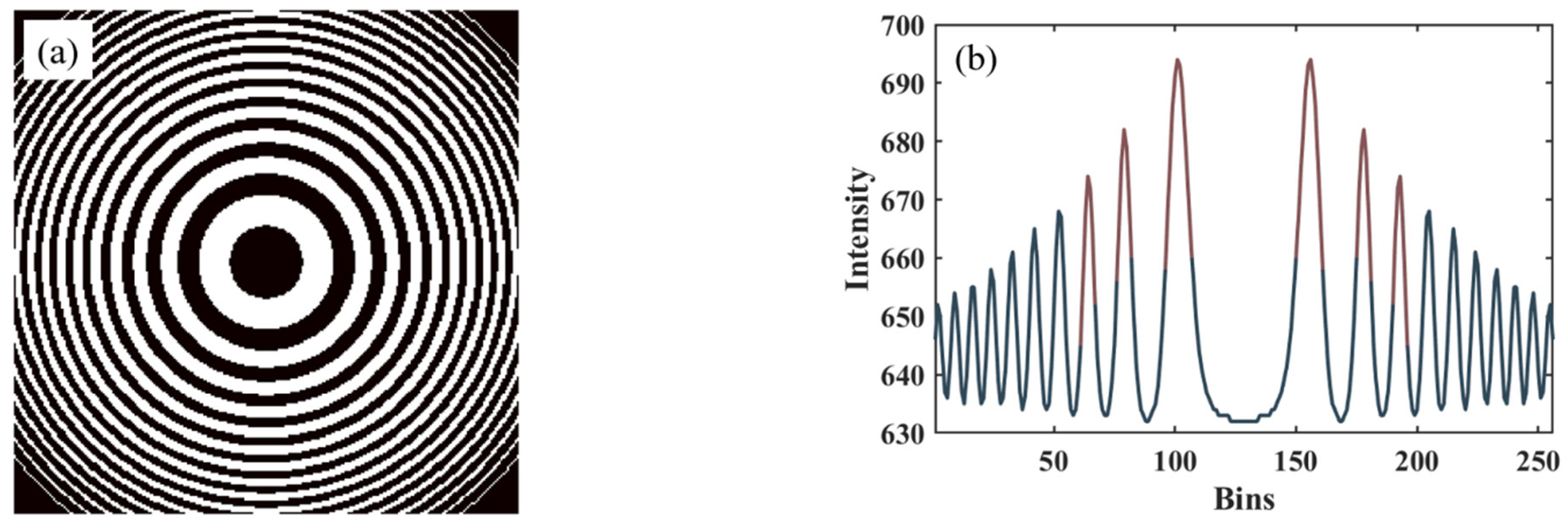
Binarization. The method thresholds the interferogram and fits rings to obtain the center, as shown in Figure 2a. The median value of all pixels in the image is taken as the threshold. Multiple rings can be fitted simultaneously to improve the stability.

(2)

Peak fitting. First, the raw images are filtered using a median filter. [17] Then, the approximate location of the center is determined manually, and a row of pixels is taken out near it to fit each peak, as shown in Figure 2b. The mean of the two peaks of the same order ring is the horizontal coordinate of the center. Similarly, the vertical coordinates can also be obtained. If only one row or column is used to determine the center position, the results will be biased easily due to noise. We used 21 rows and columns in the actual calculation.

The interference pattern is first formed by the etalon, and then a 2D interferogram is made on the CCD camera; it is difficult to directly invert the wind speed and temperature. Therefore, we apply an annular summation to convert the 2D image into 1D [17,26]. Annular summation is used to divide the interferogram into a predetermined number of rings (bins in the 1D interferogram), the center of which is the interferogram center derived above. The mean value of the pixels in each ring is calculated and the mean values of these rings form the 1D interferogram. The 1D interferogram is a function of radius $r$ and can be described using Equation (11).

The Equation (11) is discretized and rewritten as

$$\widehat{I}(r_i)={\displaystyle \sum _{j=1}^W\widehat{A}(r_i,{\lambda }_j)Y({\lambda }_j)\Delta \lambda }+B$$

(12)

where $W$ is the amount of wavelength discretization, and $i$ is the $i$th bin of the 1D interferogram. The discretized instrument function is

$$\widehat{A}(r_i,{\lambda }_j)={\displaystyle \sum _{k=1}^{R}b(s_k,r_i)A(s_k,{\lambda }_j)\Delta s_k}$$

(13)

Equation (12) is used to fit the 1D interferogram for determining those coefficients. Finally, we can obtain the wind speed and temperature implied in the airglow interferogram. The details can be read in Ref. [19]. We use 95% confidence intervals as the error of the calculated results.

3. Effect of the Center Errors on Wind and Temperature Inversions

Significant errors will be introduced into the inversion results because the wrong wind and temperature are inverted for a 1D interferogram converted with an inaccurate center. We use constant values of V = 50 m/s and T = 600 K as shown in Figure 1. Figure 3 shows the variation in wind and temperature with center deviation, which refers to the distance between the real center and the center used. The error in both wind and temperature increases with the deviation. The wind is less than the true value, while the temperature is greater than that. The reader can decide the center deviation according to the requirements of their calculation accuracy, using the results in Figure 3.

4. A New Algorithm for Determining the Center

The accuracy of the interference ring center is a basis for correctly converting 2D images and has a significant impact on the wind and temperature inversion. Laser calibration and algorithms are two popular methods for determining the center of an interferogram [19,27]. Laser calibration is used to obtain high SNR interferograms with a laser of a similar wavelength as the airglow, which can be easily used to obtain the accurate center. However, this method has some drawbacks for some FPIs. Temperature variation and the vibrations generated by the sky scanner and filter wheel in the scanning FPI cause random shifts in the interferogram center. Additionally, failure of the calibration laser during automatic observation is difficult to detect in time, resulting in a large amount of data not being available. The calibrated laser of FPI in Mohe malfunctioned between January and April 2020 [15]. Therefore, it is essential to develop high-precision algorithms to obtain interferogram centers. In this section, we propose a new algorithm for determining the interferogram center. The performance of the MSDM for determining the center from noisy and distorted interferograms is investigated and compared with the two algorithms of binarization and peak fitting.

4.1. Analysis Process

We propose the maximum standard deviation method, which can accurately determine the center from interferograms. The first step is to select a point as the center and perform an annular summation to obtain the 1D interferogram. There are two ways to perform the annular summation. The first one is to ensure that each annulus has the same area, which has already been mentioned in ref. [17]. The second one is to let each annulus have the same radial width. Then, the average value of pixels in each annulus is calculated. It should be ensured that there is a sufficient number of annuli to perform the two methods. The second step is to calculate the standard deviation of the 1D interferogram. The standard deviation of the pixel intensity of the 1D interferogram is calculated after converting the 2D interferogram to 1D. The standard deviation for the 1D interferogram converted using real centers is the largest, as demonstrated below. Based on the above steps, we can adopt an iterative approach to determine the real centers. The FPI should be installed so that the interferogram center is positioned as close as possible to the center of the image to ensure that there are more complete interference rings in the image. The real center of the airglow interferogram varies randomly within a few pixel ranges by mechanical vibration, temperature variations, or other factors. Then, the center of the image is used as the initial point to select area-1 containing the center variation range. There are N points uniformly distributed in area-1, one of which forms a smaller area with the neighboring points. Therefore, different points can be chosen to form different smaller areas with neighboring points. The more points in area-1, the more smaller regions can be divided and the higher the accuracy. Calculating the standard deviation of the 1D interferogram from these N points, the point with the largest standard deviation is used as the second point to determine area-2, which is a smaller area in area-1. The standard deviation of N points reselected in area-2 is calculated again. The accuracy is improved because the size of the area is reduced while the number of points remains unchanged. The above steps are repeated until the required accuracy is achieved.

As shown in Figure 4, $o^{\prime }$ is chosen as the center for performing the annular summation, $o$ is the real interferogram center, and $l$ is the distance between the two centers. The center of the two dotted circles is $o$. The black annulus is one of the segmented ones. According to the calculus idea, we consider this annulus as a circle $c$. The average value of the pixel intensity in this region is:

$$I(r^{\prime })=\frac{{\displaystyle {\oint }_c\widehat{I}(r)}ds}{n_{r^{\prime }}}$$

(14)

where $n_{r^{\prime }}$ is the number of pixels. When $l$ is not zero, $I(r^{\prime })$ cannot reach the peaks at the brightest and darkest for any $r^{\prime }$. This is the average of $\widehat{I}(r)$ between $r^{\prime }-l$ and $r^{\prime }+l$ (the annulus is between two dashed circles), which means that $I(r^{\prime })$ is smoother. When $l$ is zero, it can reach any value. Therefore, the 1D interferogram converted with the real center has the largest standard deviation.

The number of bins affects the accuracy of the MSDM in determining the center. Two hundred images identical to Figure 1 are generated, except for the location of the center. The results of the experiment are shown in Figure 5. When the number of bins is small, the error is large. If the number of bins is more than 100, the mean value is less than 0.05 pixels, which is higher than the accuracy required to invert the wind speed and temperature.

4.2. The MSDM Performance on Noisy and Distortion Interferograms

The airglow is very dim, coupled with absorption and scattering by the atmosphere, so the intensity of the airglow on the ground is even weaker. The intensity of the signal received by FPI is greatly reduced on the cloudy and rainy days, resulting in a low SNR of the airglow interferogram. Low SNR airglow interferograms severely degrade the accuracy of wind and temperature inversions. Therefore, five hundred images are generated for each type of noise by adding different intensities of Gaussian white noise and Poisson noise to Figure 1. We derive the centers, respectively, using the three algorithms from these images, which are used to invert the wind and temperature.

4.2.1. Gaussian White Noise

Gaussian white noise in interferograms is an essential influence on ground-based FPI observation, which is caused by the atmosphere and background light, etc. Figure 6 shows the centers determined by the MSDM, binarization, and peak fitting, respectively, as well as the wind and temperature inverted with them. The error of the center derived with the MSDM is small, less than 0.05 pixels. Both wind and temperature distributions are symmetric to the real value and approach the real value as the signal-to-noise ratio (SNR) increases. This distribution differs from the distribution of results due to central error, as shown in Figure 3. When the SNR is less than 97 dB, the deviation of binarization is too large to invert the result. The wind is less than the real value and the temperature is greater than the real value, all of which can be explained by Figure 3. The error of the peak fitting is less than 0.8, which is better than the binarization. Therefore, binarization has the worst performance. The MSDM and peak fitting are similar in wind speed, while the temperature distribution of the MSDM at low SNR is 500~750 K, which is less than the 500~900 K of the peak fitting. When the SNR of the images is high, all three algorithms can obtain accurate centers.

4.2.2. Poisson Noise

We add Poisson noise to the interferogram because the observation is also limited by photon noise. The intensity of Poisson noise is related to the gray value of the image. Figure 7 shows the interferogram center, wind, and temperature derived using the three algorithms. All three algorithms work well at higher signal intensity. The binarization remains the worst at low SNR and the MSDM has a slight advantage over the peak fitting.

4.3. Distortion Interferograms

In addition to being affected by different types of noise, the interferogram is also distorted by moonlight and strong background light. Distortions can also introduce errors in the wind and temperature inversion. Figure 8a shows the airglow interferogram recorded by the FPI deployed in Kelan. The upper part of the picture may be affected by the strong background light, which is not an accidental situation. To simulate the distortion, we assume that the simulated distortion interferogram is generated by:

$$\begin{array}{c}{I}_d(x,y)=\widehat{I}(x,y)+\hfill \\ \hspace{1em}\hspace{1em}\hspace{1em} K\frac{1}{2\pi {\sigma }_1{\sigma }_2\sqrt{1-{\rho }^2}}\exp \left[-\frac{1}{2(1-{\rho }^2)}(\frac{{(x-{\mu }_1)}^2}{{\sigma }_1^2}-\frac{2\rho (x-{\mu }_1)(y-{\mu }_2)}{{\sigma }_1{\sigma }_2}+\frac{{(y-{\mu }_2)}^2}{{\sigma }_2^2})\right]\end{array}$$

(15)

where ${\mu }_1$, ${\mu }_2$, ${\sigma }_1$, ${\sigma }_2$ and $\rho$ are horizontal coordinates, and $K$ controls the level of distortion. From the interferogram with K = 7 in Figure 8b, it can be seen that the characteristics of the distortion interferogram are well simulated.

Figure 9 shows the interference ring center determined by the three algorithms. The center determined by the binarization is completely wrong. A suitable threshold cannot be found to divide the images. The deviations of the MSDM and peak fitting are less than 0.08 and 0.02, respectively.

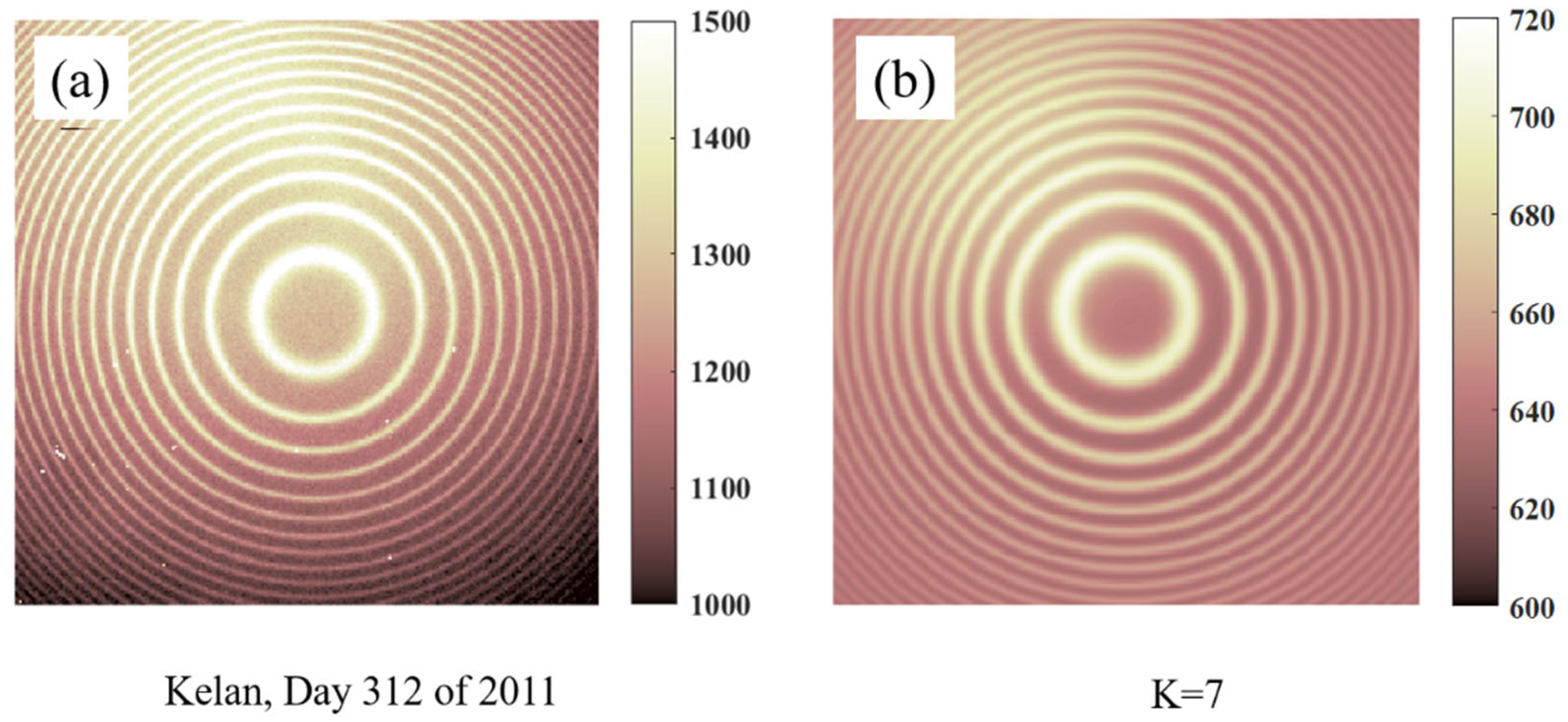
5. Application to Wind and Temperature Inversion from Real Airglow Interferograms

The FPI in Kelan is manufactured by the National Center for Atmospheric Research (NCAR). The Kelan FPI mainly includes a control system, dome, sky scanner, filter wheel, standard gear, lens, and camera. The National Center for Atmospheric Research used to calibrate it and perform trial runs, so data inversion software is available. It has been in stable operation at Kelan for several years and is currently in a state of repair. We use the airglow interferogram obtained by this FPI to test the performance of the algorithm. Figure 10 only shows the inversion by the MSDM and peak fitting, as well as a comparison with the FPI product. The interferograms of this day are distorted, and the wind and temperature inverted by using binarization are completely wrong. For the zonal wind, the three inversions are generally consistent with very little deviation, except for a very large deviation in the peak fitting at 19 h. The peak fitting inversion of the meridional wind is greater than 150 m/s at 18 h. For temperature, the deviation in MSDM is less than 50 K, while the deviation in the peak fitting exceeds 250 K at both 18 and 19 h. The wind and temperature deviations are at their maximum at 18 h, which means that the quality of the interferogram is low. Finally, we can see that the signal intensity first decreases and then increases, and is lowest at 18 and 19 h. Signal intensity is susceptible to atmospheric and other factors, thus reducing the SNR of airglow interferograms. The wind and temperature errors prove each other with the signal intensity. It is also demonstrated that the MSDM has better stability than peak fitting at low SNR.

6. Summary

We propose the MSDM for determining the center of the 2D interferogram before converting it to a 1D interferogram, by which the wind and temperature in the middle and upper atmosphere can be estimated. To check the performance of the MSDM algorithm, an analysis procedure was performed using simulation interferograms. First, we describe a forward model based on the revised model to create 2D interferograms. The 2D interferogram is then converted to 1D using annular summation. Finally, the linear regression algorithm corresponding to the forward model is used to invert wind and temperature from 1D interferograms.

Inaccurate center deviations can result in errors in wind and temperature [17]. By presenting the errors for various center deviations, we enable readers to select the appropriate level of precision based on their specific accuracy requirements. After calculating 200 images, it is found that the number of bins of 1D interferograms should be more than 100 to fully achieve the performance of the MSDM. Next, we add Gaussian white noise, Poisson noise, and distortion to the interferogram to create 500 images to study the stability of the algorithm. At the same time, binarization and peak fitting, which are currently widely used, are used as comparisons.

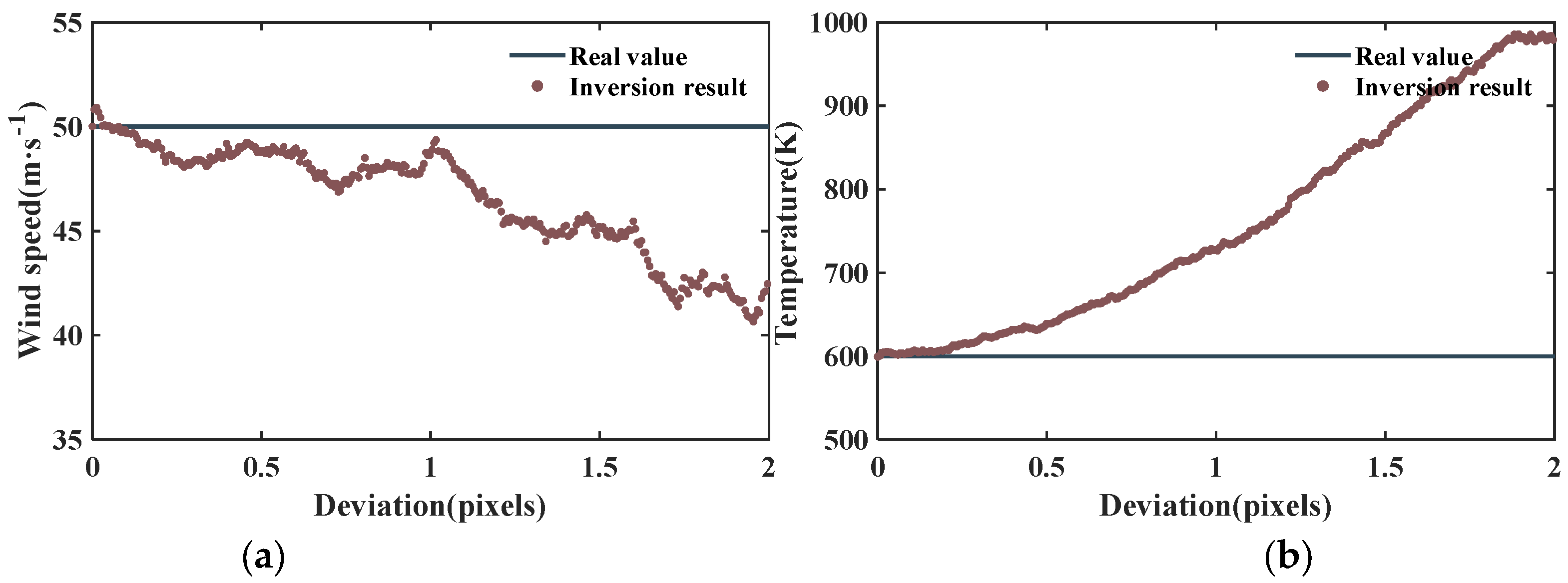
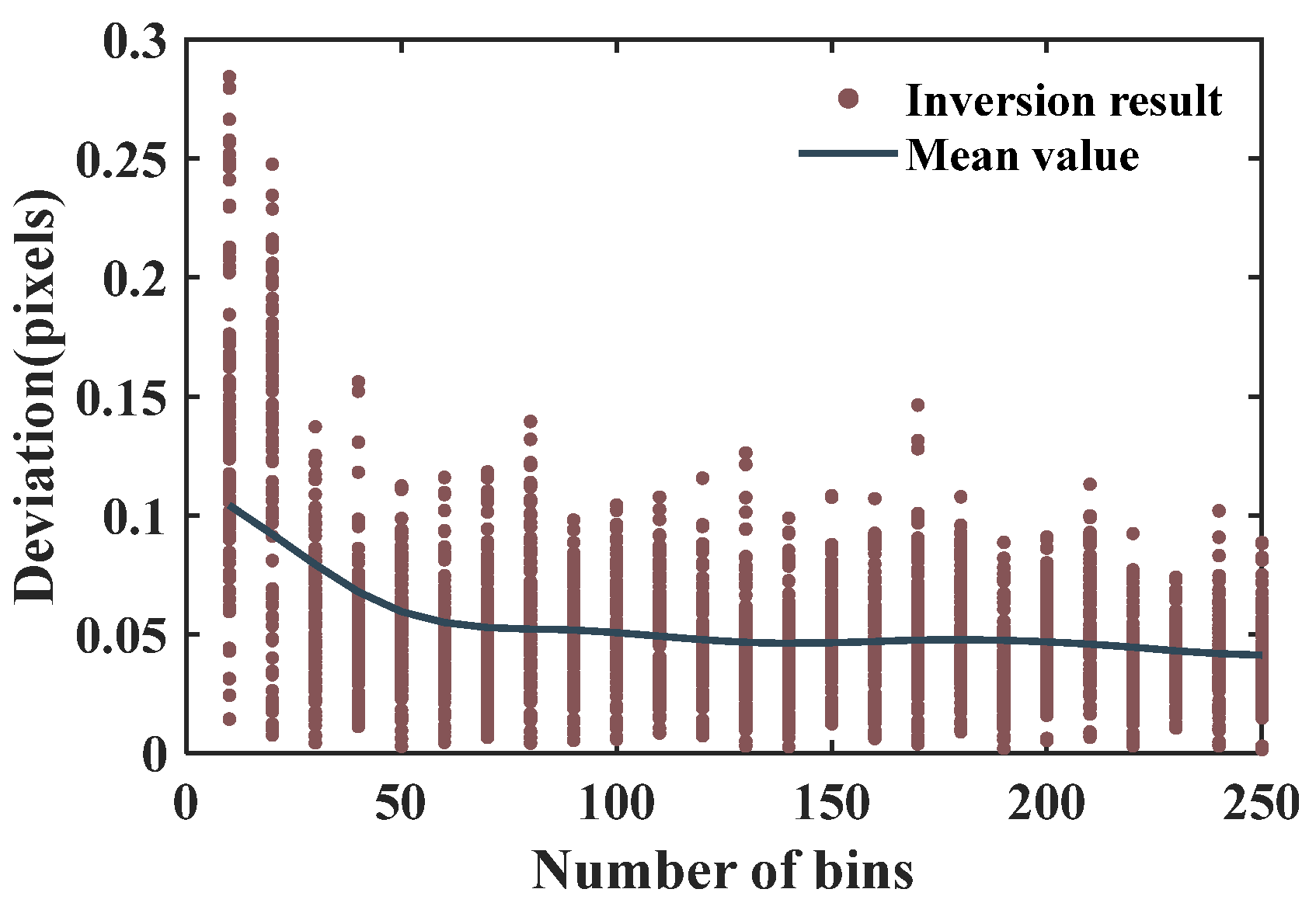
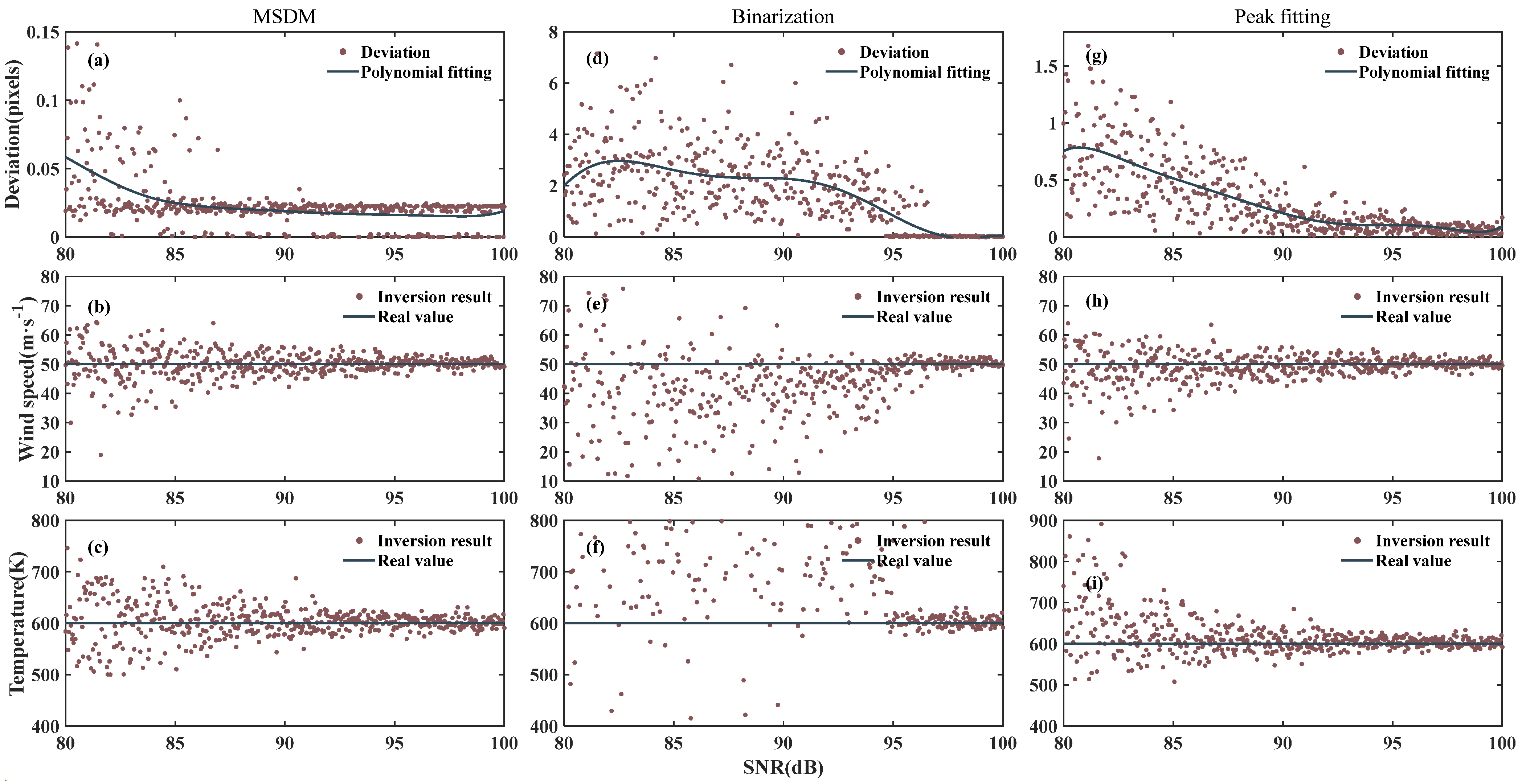
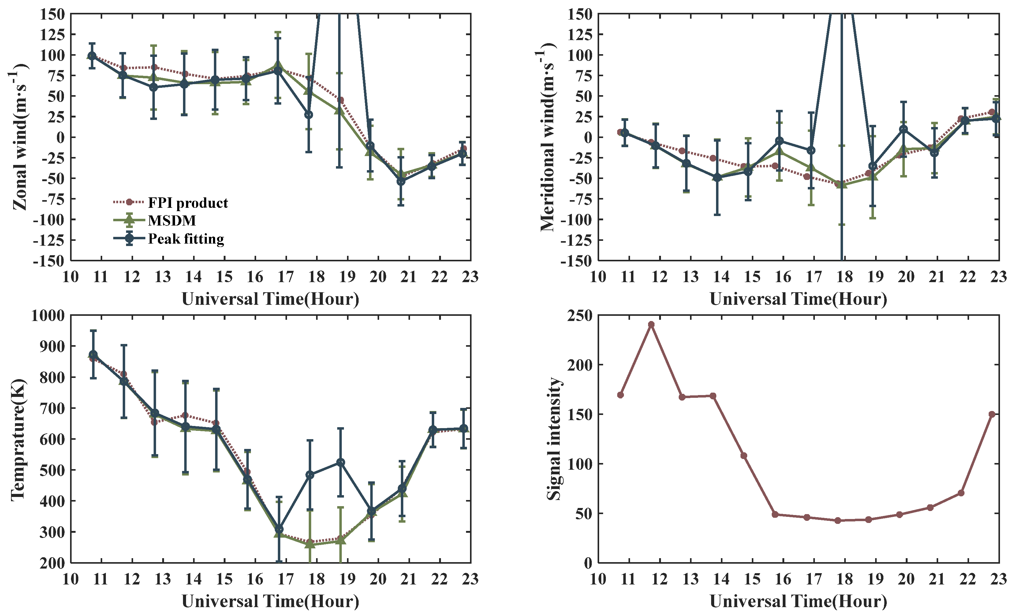
• For Poisson noise, the center deviation of the MSDM is less than 0.05 pixels. The SNR of the images has a great influence on binarization and peak fitting, so more accurate results can only be obtained from high-quality images. Especially for temperature, the MSDM results are in the range of 500 to 750 K.
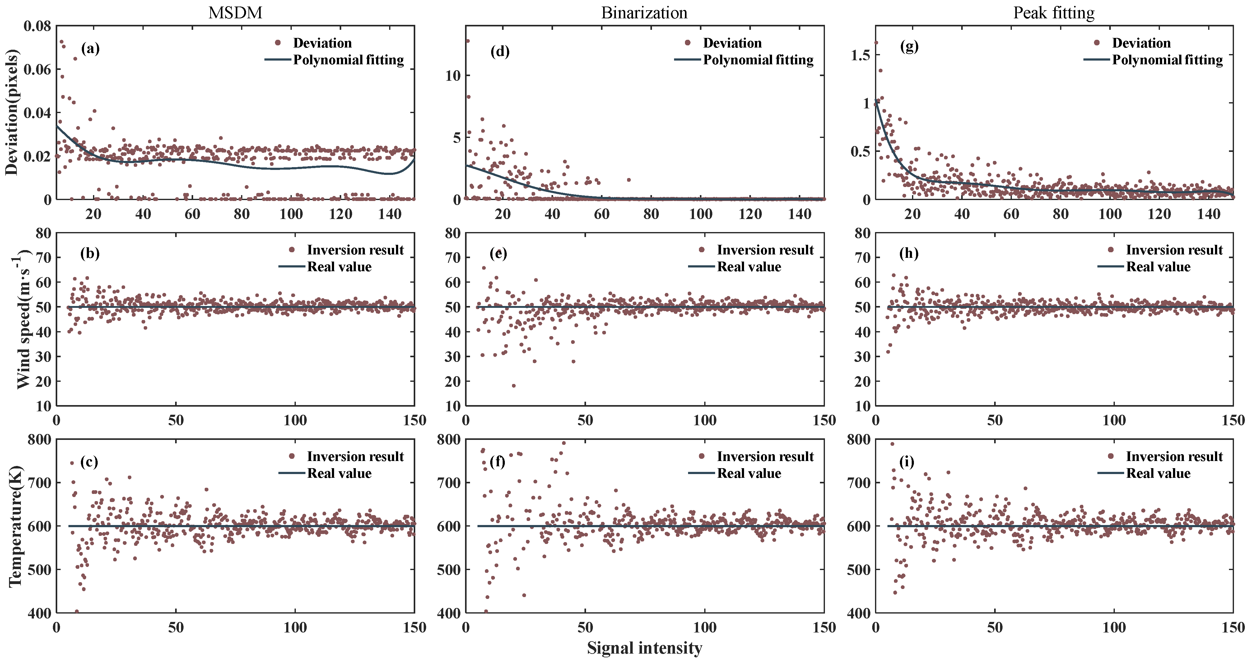
• For Poisson noise, the performance of the MSDM maintains very good performance for different signal intensities. However, binarization and peak fitting are more affected by noise.
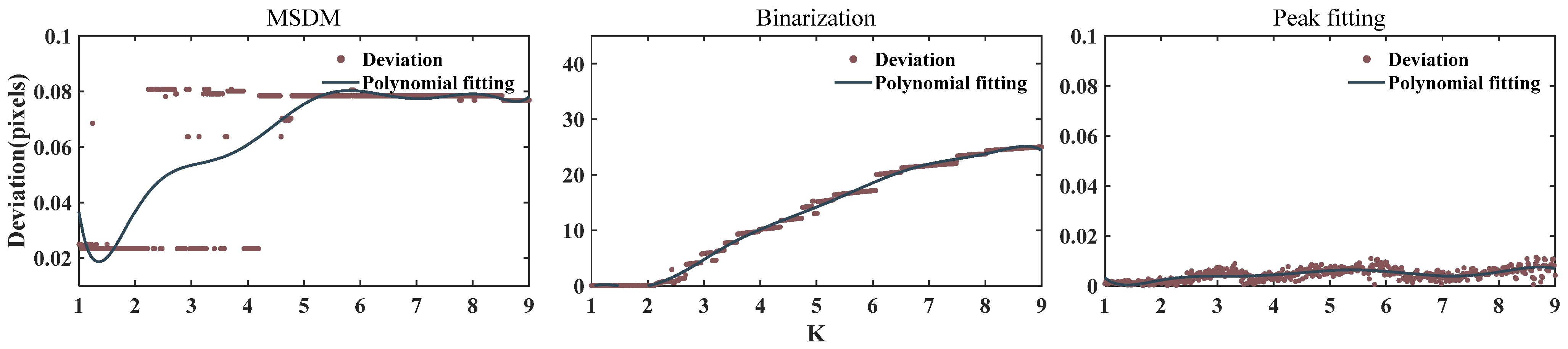
• For distortion interferograms, the binarization method calculates completely wrong centers, while the MSDM and peak fitting give more accurate results.

From the above experiments, the MSDM shows high accuracy and strong stability in both distortion and various noise interferograms. The peak fitting is accurate at high SNR, but the approximate center needs to be determined manually before calculation. Finally, we invert the wind and temperature from airglow interferograms observed by Kelan FPI. The calculation using binarization fails due to the distortion of the airglow interferogram. For high SNR images, the MSDM and peak fitting coincide well with the FPI product. For low SNRs, the MSDM better agrees well with the results of the FPI product. This demonstrates that the MSDM is not only accurate but also highly robust for automatically performance.

References

1. Chapagain, N.P.; Makela, J.J.; Meriwether, J.W.; Fisher, D.J.; Buriti, R.A.; de Medeiros, A.F. Comparison of nighttime zonal neutral winds and equatorial plasma bubble drift velocities over Brazil: Zonal neutral winds and epb velocities. J. Geophys. Res. Atmos. 2012, 117, A06309. [Google Scholar] [CrossRef]
2. Sarudin, I.; Hamid, N.S.A.; Abdullah, M.; Buhari, S.M.; Shiokawa, K.; Otsuka, Y.; Hozumi, K.; Jamjareegulgarn, P. Influence of Zonal Wind Velocity Variation on Equatorial Plasma Bubble Occurrences Over Southeast Asia. J. Geophys. Res. Space Phys. 2021, 126, e2020JA028994. [Google Scholar] [CrossRef]
3. Rabiu, A.B.; Okoh, D.I.; Wu, Q.; Bolaji, O.S.; Abdulrahim, R.B.; Dare-Idowu, O.E.; Obafaye, A.A. Investigation of the Variability of Night-Time Equatorial Thermospheric Winds Over Nigeria, West Africa. J. Geophys. Res. Space Phys. 2021, 126, e2020JA028528. [Google Scholar] [CrossRef]
4. Navarro, L.A.; Fejer, B.G. Storm-Time Thermospheric Winds Over Peru. J. Geophys. Res. Space Phys. 2019, 124, 10415–10427. [Google Scholar] [CrossRef] [Green Version]
5. Grawe, M.A.; Chu, K.T.; Makela, J.J. Measurement of atmospheric neutral wind and temperature from Fabry-Perot interferometer data using piloted deconvolution. Appl. Opt. 2019, 58, 3685–3695. [Google Scholar] [CrossRef]
6. Liu, X.; Xu, J.; Zhang, S.; Jiang, G.; Zhou, Q.; Yuan, W.; Noto, J.; Kerr, R. Thermospheric planetary wave-type oscillations observed by FPIs over Xinglong and Millstone Hill. J. Geophys. Res. Space Phys. 2014, 119, 6891–6901. [Google Scholar] [CrossRef]
7. Liu, Y.; Xu, J.; Liu, X.; Zhang, S.; Yuan, W.; Liu, W.; Wu, K.; Wang, C. Responses of Multiday Oscillations in the Nighttime Thermospheric Temperature to Solar and Geomagnetic Activities Measured by Fabry-Perot Interferometer in China. J. Geophys. Res. Space Phys. 2019, 124, 9420–9429. [Google Scholar] [CrossRef]
8. Koomen, M.J.; Gulledge, I.S.; Packer, D.M.; Tousey, R. Night Airglow Observations from Orbiting Spacecraft Compared with Measurements from Rockets. Science 1963, 140, 1087–1089. [Google Scholar] [CrossRef]
9. Sparrow, J.G.; Ney, E.P.; Burnett, G.B.; Stoddart, J.W. Airglow observations from OSO-B2 satellite. J. Geophys. Res. 1968, 73, 10. [Google Scholar] [CrossRef]
10. Chamberlain, J.W. Physics of the Aurora and Airglow: International Geophysics Series; Elsevier: Amsterdam, The Netherlands, 2016; Volume 2. [Google Scholar]
11. Shiokawa, K.; Kadota, T.; Ejiri, M.K.; Otsuka, Y.; Katoh, Y.; Satoh, M.; Ogawa, T. Three-channel imaging fabry-perot interferometer for measurement of mid-latitude airglow. Appl. Opt. 2001, 40, 4286. [Google Scholar] [CrossRef]
12. Shiokawa, K.; Otsuka, Y.; Oyama, S.; Nozawa, S.; Satoh, M.; Katoh, Y.; Hamaguchi, Y.; Yamamoto, Y.; Meriwether, J. Development of low-cost sky-scanning Fabry-Perot interferometers for airglow and auroral studies. Earth Planets Space 2012, 64, 1033–1046. [Google Scholar] [CrossRef] [Green Version]
13. Wang, H.; Wang, Y.; Fu, J. A Tiny Fabry-Perot Interferometer with Postpositional Filter for Measurement of the Thermospheric Wind. Acta Geophys. 2016, 64, 2748–2760. [Google Scholar] [CrossRef] [Green Version]
14. Wu, Q.; Gablehouse, R.D.; Solomon, S.C.; Killeen, T.L.; She, C.Y. A New Fabry-Perot Interferometer for Upper Atmosphere Research. In Proceedings of the Conference on Instruments, Science, and Methods for Geospace and Planetary Remote Sensing, Honolulu, HI, USA, 9–11 November 2004. [Google Scholar]
15. Li, W.; Chen, Y.; Liu, L.; Trondsen, T.S.; Unick, C.; Wyatt, D.; Ning, B.; Li, G.; Huang, C.; Yang, S.; et al. Variations of Thermospheric Winds Observed by a Fabry–Perot Interferometer at Mohe, China. J. Geophys. Res. Space Phys. 2021, 126, e2020JA028655. [Google Scholar] [CrossRef]
16. Smith, R.W. Vertical winds: A tutorial. J. Atmos. Solar-Terr. Phys. 1998, 60, 1425–1434. [Google Scholar] [CrossRef]
17. Makela, J.J.; Meriwether, J.W.; Huang, Y.; Sherwood, P.J. Simulation and analysis of a multi-order imaging Fabry–Perot interferometer for the study of thermospheric winds and temperatures. Appl. Opt. 2011, 50, 4403. [Google Scholar] [CrossRef]
18. Huang, Y.; Makela, J.J.; Swenson, G.R. Simulations of imaging Fabry–Perot interferometers for measuring upper-atmospheric temperatures and winds. Appl. Opt. 2012, 51, 3787. [Google Scholar] [CrossRef]
19. Harding, B.J.; Gehrels, T.W.; Makela, J.J. Nonlinear regression method for estimating neutral wind and temperature from Fabry–Perot interferometer data. Appl. Opt. 2014, 53, 666–673. [Google Scholar] [CrossRef] [Green Version]
20. Hu, G.; Ai, Y.; Zhang, Y.; Zhang, H.; Liu, J. First scanning Fabry–Perot interferometer developed in China. Chin. Sci. Bull. 2014, 59, 563–570. [Google Scholar] [CrossRef]
21. Chanin, G.; Lecullier, J.C. A scanning Fabry-Perot interferometer. Infrared Phys. 1978, 18, 589–594. [Google Scholar] [CrossRef]
22. Moiseev, A.V. Scanning Fabry–Perot Interferometer of the 6-m SAO RAS Telescope. Astrophys. Bull. 2021, 76, 316–339. [Google Scholar] [CrossRef]
23. Hays, P.B.; Roble, R.G. A Technique for Recovering Doppler Line Profiles from Fabry-Perot Interferometer Fringes of Very Low Intensity. Appl. Opt. 1971, 10, 193. [Google Scholar] [CrossRef] [PubMed]
24. Hernandez, G. Analytical Description of a Fabry–Perot Photoelectric Spectrometer. Appl. Opt. 1966, 5, 1745. [Google Scholar] [CrossRef] [PubMed]
25. Hernandez, G. Analytical Description of a Fabry-Perot Photoelectric Spectrometer 2: Numerical Results. Appl. Opt. 1970, 9, 1591. [Google Scholar] [CrossRef]
26. Niciejewski, R.J.; Killeen, T.L.; Turnbull, M. Ground-based Fabry-Perot interferometry of the terrestrial nightglow with a bare charge-coupled device: Remote field site deployment. Opt. Eng. 1994, 33, 457. [Google Scholar] [CrossRef] [Green Version]
27. Vasilyev, R.V.; Artamonov, M.F.; Beletsky, A.B.; Zherebtsov, G.A.; Medvedeva, I.V.; Mikhalev, A.V.; Syrenova, T.E. Registering Upper Atmosphere Parameters in East Siberia with Fabry-Perot Interferometer KEO Scientific “Arinae”. Sol. Terr. Phys. 2017, 3, 61–75. [Google Scholar] [CrossRef] [Green Version]
Figure 1. Simulated interferogram with V = 50 m/s, T = 600 K.
Remotesensing 15 01934 g001
Figure 2. (a) Binarization and (b) peak fitting.
Remotesensing 15 01934 g002
Figure 3. (a) Wind and (b) temperature versus the deviation between the real center and the center used.
Remotesensing 15 01934 g003
Figure 4. The analysis process of the MSDM.
Remotesensing 15 01934 g004
Figure 5. The deviation of the interferogram center using the MSDM with different numbers of bins.
Remotesensing 15 01934 g005
Figure 6. The top, middle, and bottom rows show the center deviation, wind, and temperature, respectively. The left, middle, and right columns are calculated using the MSDM, binarization, and peak fitting, respectively. The wind and temperature for each method use the center with deviations in the first column.
Remotesensing 15 01934 g006
Figure 7. Same as Figure 6, but for Poisson noise.
Remotesensing 15 01934 g007
Figure 8. (a) Distorted FPI airglow interferogram (Kelan, Day 312 of 2011) and (b) simulated distortion interferogram (K = 0.1).
Remotesensing 15 01934 g008
Figure 9. The center deviation using the three algorithms.
Remotesensing 15 01934 g009
Figure 10. Inversion with airglow interferograms on day 17 of 2012. Wind and temperature errors and signal intensity provided by FPI products manufactured by NCAR.
Remotesensing 15 01934 g010
Disclaimer/Publisher’s Note: The statements, opinions and data contained in all publications are solely those of the individual author(s) and contributor(s) and not of MDPI and/or the editor(s). MDPI and/or the editor(s) disclaim responsibility for any injury to people or property resulting from any ideas, methods, instructions or products referred to in the content.