
Radiometric Terrain Flattening of Geocoded Stacks of SAR Imagery

Abstract
:1. Introduction
Terminology
- A geocoded product or Geocoded Terrain-Corrected (GTC) product, as referenced in the SAR mission product user guides, is derived by precisely geolocating SAR imagery using a Digital Elevation Model (DEM) [7]. Alternately, the GTC products themselves could be generated directly by focusing raw radar pulses onto a regular map grid [8]. When starting from Level-1 products, SAR imagery is usually calibrated to before it is interpolated onto a regular map grid. Please note that the subscript E in indicates that the radiometry of the product has been adjusted under the assumption that the area being imaged lies on the reference ellipsoid or a well-defined flat reference surface. GTC products calibrated to or are also common. GTC products have been geolocated precisely [9] but have not been corrected for terrain-related radiometric effects. Although we have provided mathematical expressions for working with different calibration levels of GTC products in this manuscript, we specifically focus on GTC products, which we process at Descartes Labs at a global scale [10].
- A terrain-flattened or Radiometrically Terrain-Corrected (RTC) product [4] or normalized radar backscatter (NRB) [11] product is a special type of GTC product where the imagery has been corrected for terrain-related radiometric effects. In the context of this manuscript, we always assume that an RTC product has been calibrated to (Table I of [4]). RTC products are widely considered to be the most ready-for-analysis product derived from SAR imagery and most similar to optical imagery for developing similar applications [1,11]. The difference between GTC and RTC products is that the radiometry of GTC products corresponds to the reference ellipsoid or a reference flat surface and the radiometry of RTC products corresponds to the actual terrain represented by a DEM.
- In general, a collection of GTC products generated on the same map grid is referred to as a geocoded stack. In the context of this manuscript, we specifically refer to GTC products generated on a common grid from interferometrically compliant acquisitions as a geocoded stack, unless mentioned otherwise. Such products are usually labeled with a common Path-Frame identifier (ERS, ALOS, etc.) or unique burst identifiers (Sentinel-1) [10,12]. These identifiers represent unique imaging geometry configurations, i.e., all images in the collection share baselines of less than a few kilometers with respect to each other and are acquired at similar incidence angles.
2. Revisiting the Gamma Flattening Formulation
2.1. Single DEM Facet
- Equation (1) can be used to flatten GTC products corresponding to any of the standard calibration levels—, and .
- The formulation can be applied to GTC products in any well-known map projection system [14] as long as the actual area computations are performed in a 3-D geocentric cartesian projection system, e.g., EPSG:4978, to avoid projection system related distortions.
- Since the transformation of GTC products according to Equation (1) only involves computation of simple facet-by-facet area normalization factors (assuming no layover), we can significantly speed up processing and circumvent the use of large radar image index lookup tables.
2.2. Extension to Rectangular Pixels
3. Terrain Flattening of Geocoded Stacks
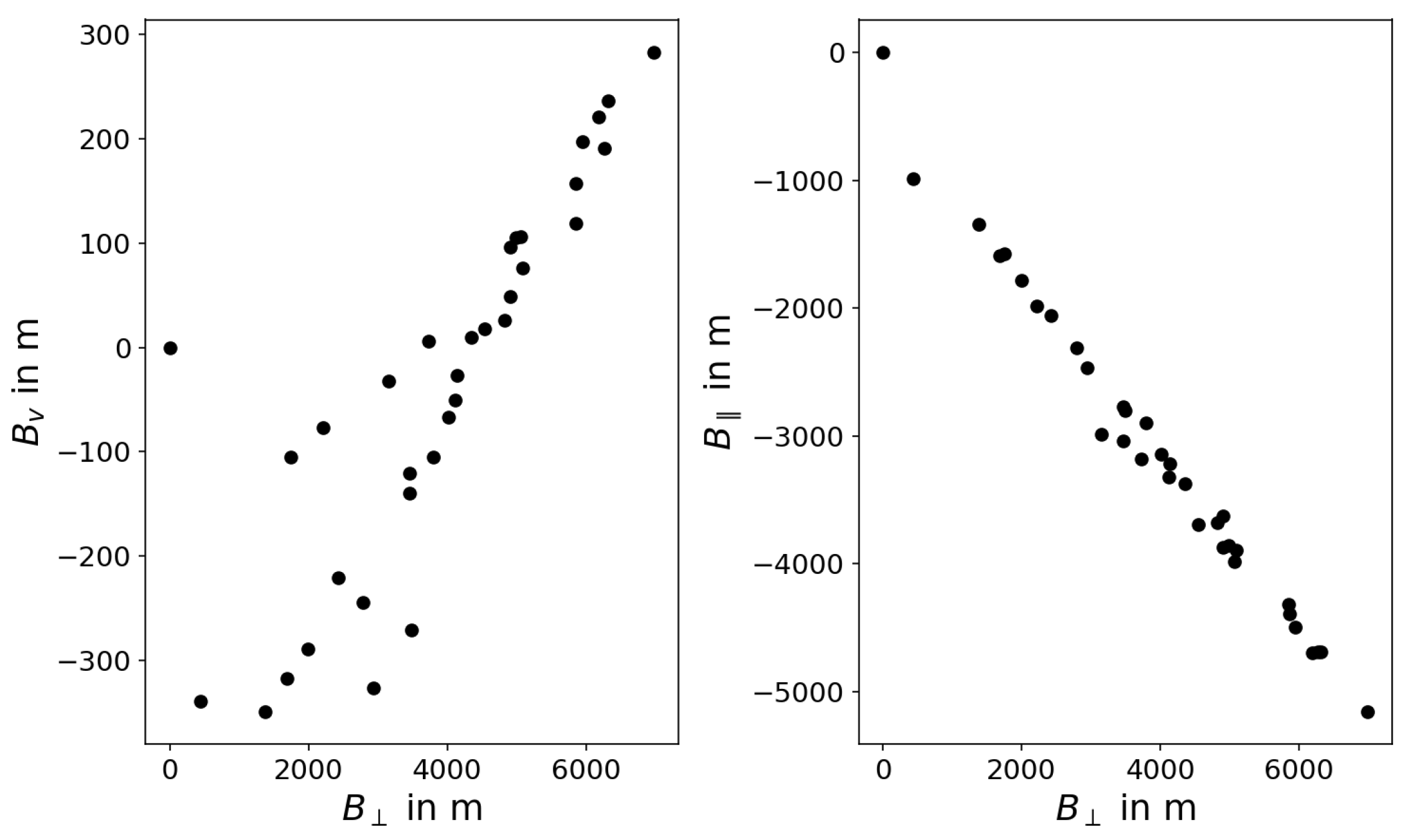
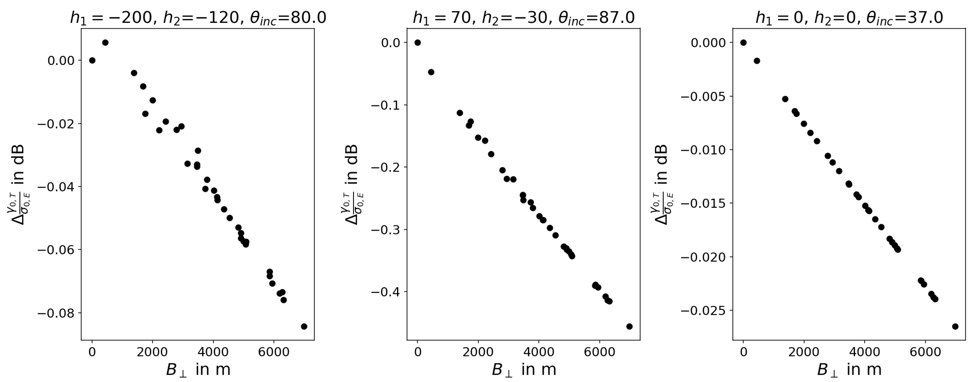
3.1. Sentinel-1
3.2. ALOS-1
3.3. Generalized Formulation
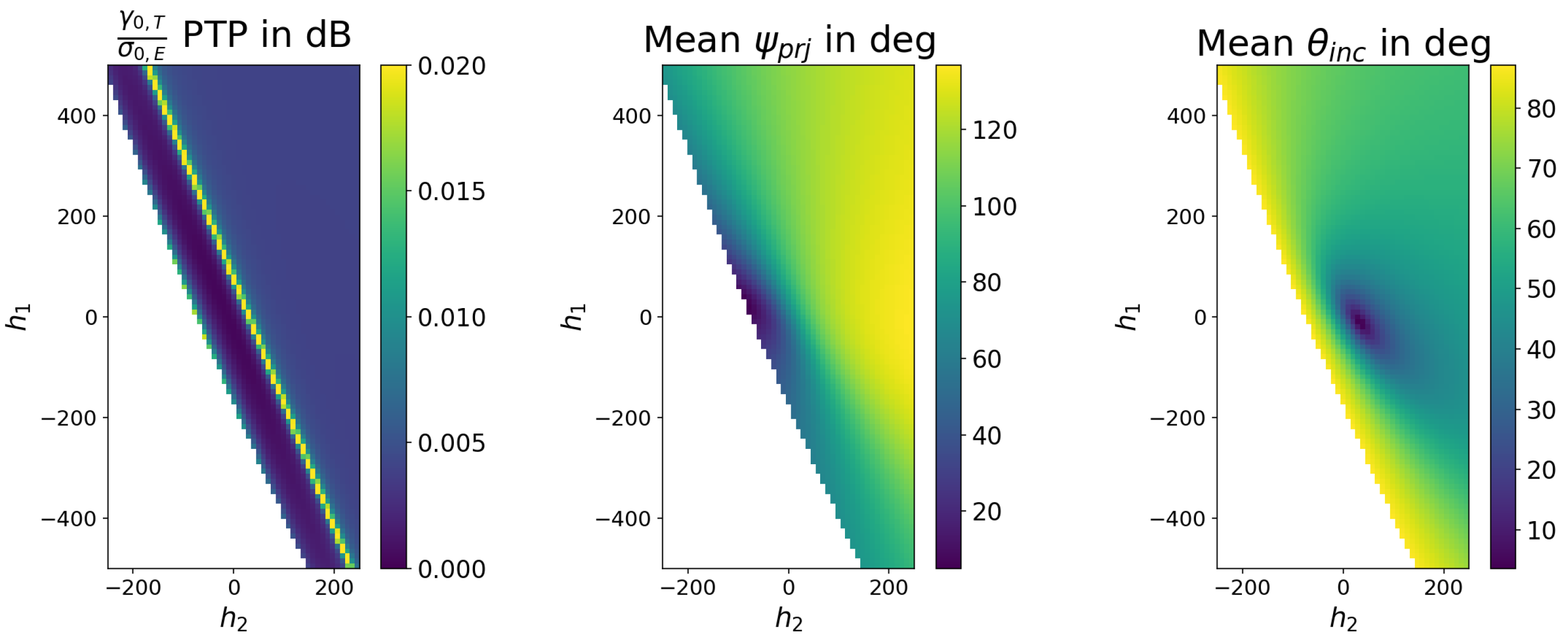
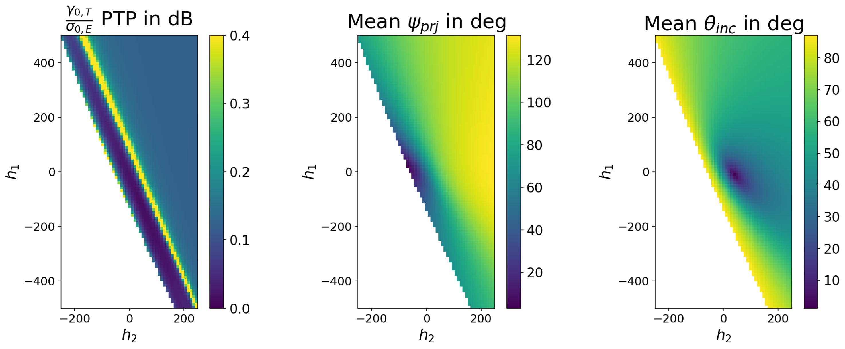
4. Impact of Layover
4.1. Single SAR Image
4.2. Stack of SAR Images
4.3. Shadow–Layover Mask
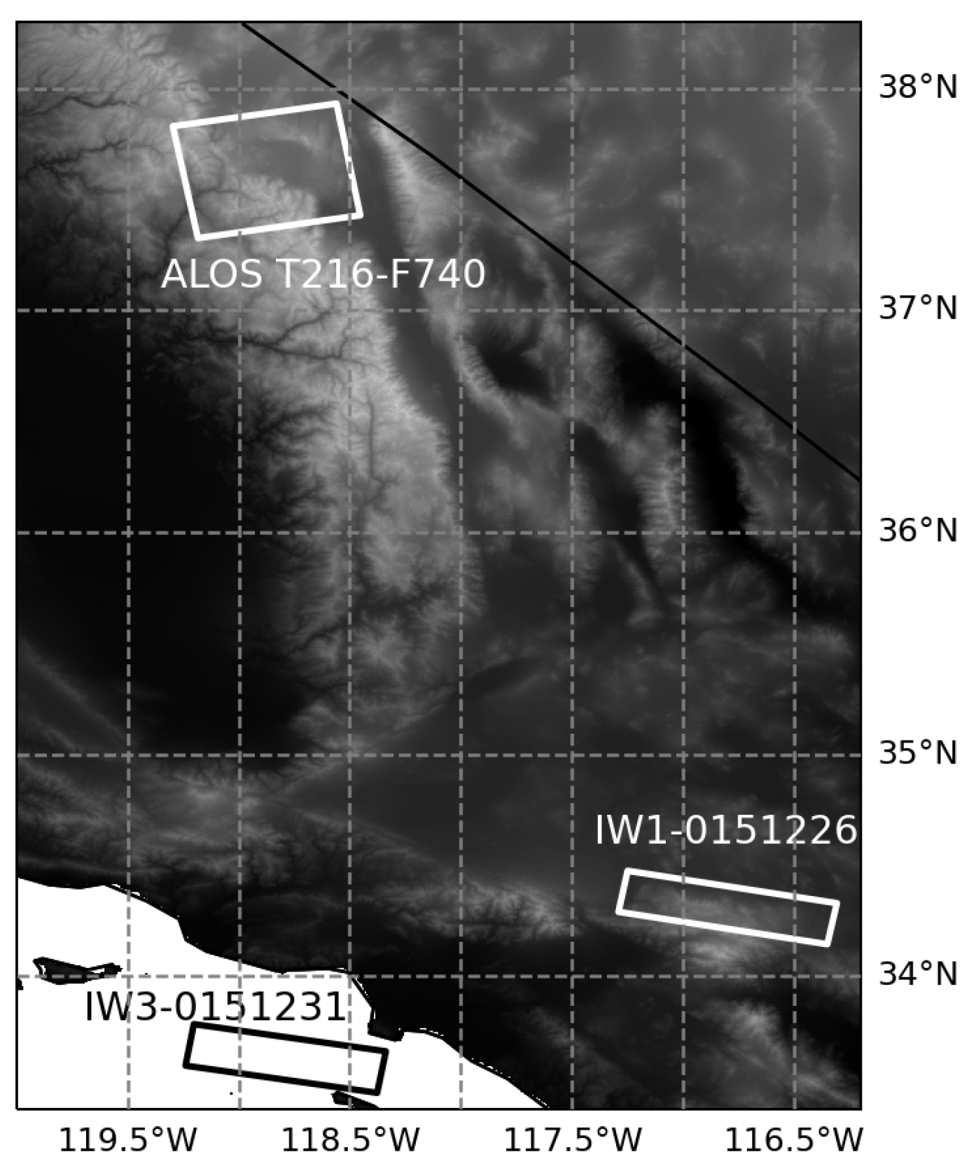
5. Experiments with the Sentinel-1 Toolbox
- The elimination of the effect of differences introduced by InSAR-grade interpolators [33] used in the complex-value interpolation of SLC data and noisier bilinear or bicubic interpolators used with real-valued intensity data in the workflow, letting us focus on geometric inconsistencies.
- A GTC product derived from a constant DN image in slant-range coordinates, which will also be a constant-valued image, thus allowing us to compare outputs with terrain-flattened products generated from GTC products as described in Section 2.
- The elimination of the effects introduced by inconsistent spatial averaging due to the use of a multilooking operator in slant-range coordinates, as multilooked products of constant DN images are also constantly valued. This effect is similar to phase-closure artifacts observed in pair-by-pair InSAR analysis as described in [10].
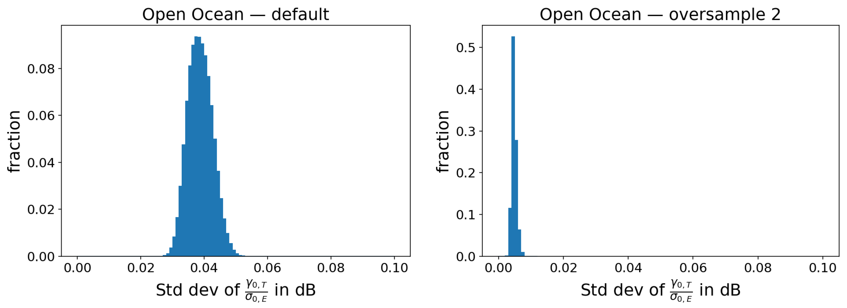
5.1. Open Ocean
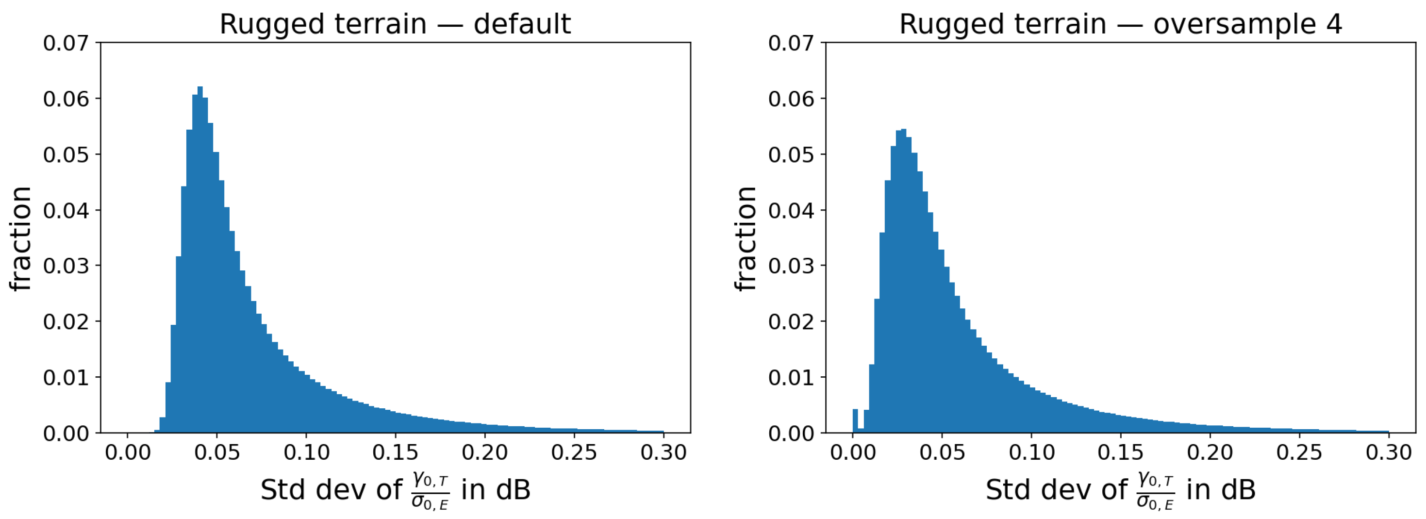
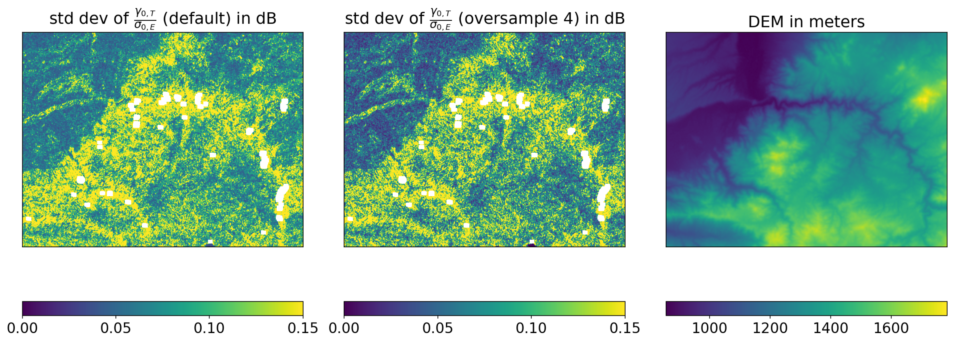
5.2. Rugged Terrain
5.3. Global Terrain-Flattening Product
- Static factor to transform to in decibel space.
- Shadow–layover mask
6. Discussion
6.1. Applicability of Terrain Flattening
- Equations (1) and (3) clearly show that terrain flattening can be considered to be a correction of a pixel-by-pixel bias term. Consequently, if the analysis of individual SAR backscatter products can be reformulated as a ratio of polarization channels, e.g., radar vegetation indices, then the terrain-flattening effects are canceled out. Such analysis can be directly performed on GTC products.
- Section 3.1 shows that the pixel-by-pixel bias is consistent for narrow orbital tube missions. Consequently, if multi-temporal backscatter analysis can be reformulated to work with relative changes regarding a reference epoch or a temporal average, terrain-flattening effects are canceled out. This is similar to using a reference epoch in InSAR time-series analysis.
- Terrain-flattened products from different imaging geometries, e.g., ascending vs. descending passes, are not necessarily comparable over heterogeneous terrain such as urban areas, where the scattering mechanism is not necessarily distributed in nature. Comparing GTC products acquired from similar imaging geometries would allow for more sensitive change detection.
- Multi-temporal and multi-modal change-detection frameworks are becoming increasingly popular for wide-area monitoring and change-detection applications, e.g., [29,34]. These frameworks are designed to analyze time-series from multiple types of sensors and combine change detections. The sensitivity of change detection from SAR data can be improved just by considering different imaging geometries as different sensors in such frameworks.
6.2. Efficient Processing
6.3. Validation of Terrain-Flattening Processors
6.4. Analysis-Ready Data Interoperability
- Normalized Radar Backscatter (NRB)
- Interferometric Radar (InSAR)
- Geocoded Single-Look Complex (GSLC)
- Polarimetric Radar (POL)
- Ocean Radar Backscatter (ORB)
6.5. Common Framework with InSAR
7. Conclusions
Author Contributions
Funding
Data Availability Statement
Acknowledgments
Conflicts of Interest
Appendix A
References
- Truckenbrodt, J.; Freemantle, T.; Williams, C.; Jones, T.; Small, D.; Dubois, C.; Thiel, C.; Rossi, C.; Syriou, A.; Giuliani, G. Towards Sentinel-1 SAR analysis-ready data: A best practices assessment on preparing backscatter data for the cube. Data 2019, 4, 93. [Google Scholar] [CrossRef] [Green Version]
- Torres, R.; Snoeij, P.; Geudtner, D.; Bibby, D.; Davidson, M.; Attema, E.; Potin, P.; Rommen, B.; Floury, N.; Brown, M.; et al. GMES Sentinel-1 mission. Remote Sens. Environ. 2012, 120, 9–24. [Google Scholar] [CrossRef]
- Dyke, G.; Rosenqvist, A.; Killough, B.; Yuan, F. Intercomparison of Sentinel-1 Datasets from Google Earth Engine and the Sinergise Sentinel Hub Card4L Tool. In Proceedings of the IEEE International Geoscience and Remote Sensing Symposium (IGARSS 2021), Brussels, Belgium, 11–16 July 2021; pp. 1796–1799. [Google Scholar] [CrossRef]
- Small, D. Flattening Gamma: Radiometric Terrain Correction for SAR Imagery. IEEE Trans. Geosci. Remote Sens. 2011, 49, 3081–3093. [Google Scholar] [CrossRef]
- Shiroma, G.H.; Lavalle, M.; Buckley, S.M. An area-based projection algorithm for SAR radiometric terrain correction and geocoding. IEEE Trans. Geosci. Remote Sens. 2022, 60, 1–23. [Google Scholar] [CrossRef]
- Veci, L.; Lu, J.; Foumelis, M.; Engdahl, M. ESA’s Multi-mission Sentinel-1 Toolbox. In Proceedings of the EGU General Assembly Conference Abstracts, Vienna, Austria, 23–28 April 2017; p. 19398. [Google Scholar]
- Meier, E.; Frei, U.; Nüesch, D. Precise terrain corrected geocoded images. In SAR Geocoding: Data and Systems; Herbert Wichman: Karlsruhe, Germany, 1993; pp. 173–185. [Google Scholar]
- Zebker, H.A. User-Friendly InSAR Data Products: Fast and Simple Timeseries Processing. IEEE Geosci. Remote Sens. Lett. 2017, 14, 2122–2126. [Google Scholar] [CrossRef]
- Small, D.; Schubert, A. Guide to ASAR geocoding. In ESA-ESRIN Technical Note RSL-ASAR-GC-AD; University of Zurich: Zurich, Switerland, 2008; Volume 1, p. 36. [Google Scholar]
- Agram, P.S.; Warren, M.S.; Calef, M.T.; Arko, S.A. An Efficient Global Scale Sentinel-1 Radar Backscatter and Interferometric Processing System. Remote Sens. 2022, 14, 3524. [Google Scholar] [CrossRef]
- CEOS CARD4L Normalized Radar Backscatter Committee. Analysis Ready Data For Land: Normalized Radar Backscatter, Version 5.5; Technical Report CARD4L-PFS_NRB_v5.5; Committee on Earth Observation Satellites: Reston, VA, USA, 2021. [Google Scholar]
- Sentinel-1 Mission Performance Cluster. Sentinel-1 Burst Id map, Version 20220530; Generated by Sentinel-1 SAR MPC. 2022. Available online: https://sar-mpc.eu/test-data-sets/ (accessed on 1 January 2023).
- Ulander, L. Radiometric slope correction of synthetic-aperture radar images. IEEE Trans. Geosci. Remote Sens. 1996, 34, 1115–1122. [Google Scholar] [CrossRef]
- PROJ Contributors. PROJ Coordinate Transformation Software Library; Open Source Geospatial Foundation: Chicago, IL, USA, 2022. [Google Scholar] [CrossRef]
- Sandwell, D.; Mellors, R.; Tong, X.; Wei, M.; Wessel, P. Open radar interferometry software for mapping surface Deformation. EOS Trans. Am. Geophys. Union 2011, 92, 234. [Google Scholar] [CrossRef] [Green Version]
- Rosen, P.A.; Gurrola, E.M.; Agram, P.; Cohen, J.; Lavalle, M.; Riel, B.V.; Fattahi, H.; Aivazis, M.A.; Simons, M.; Buckley, S.M. The InSAR Scientific Computing Environment 3.0: A Flexible Framework for NISAR Operational and User-Led Science Processing. In Proceedings of the 2018 IEEE International Geoscience and Remote Sensing Symposium (IGARSS 2018), Valencia, Spain, 22–27 July 2018; pp. 4897–4900. [Google Scholar] [CrossRef]
- Samuele, D.P.; Filippo, S.; Orusa, T.; Enrico, B.M. Mapping SAR geometric distortions and their stability along time: A new tool in Google Earth Engine based on Sentinel-1 image time series. Int. J. Remote Sens. 2021, 42, 9135–9154. [Google Scholar] [CrossRef]
- Lavalle, M.; Shiroma, G.H.; Agram, P.; Gurrola, E.; Sacco, G.F.; Rosen, P. Plant: Polarimetric-interferometric lab and analysis tools for ecosystem and land-cover science and applications. In Proceedings of the IEEE International Geoscience and Remote Sensing Symposium (IGARSS 2016), Beijing, China, 10–15 July 2016; pp. 5354–5357. [Google Scholar]
- Navacchi, C.; Cao, S.; Bauer-Marschallinger, B.; Snoeij, P.; Small, D.; Wagner, W. Utilising Sentinel-1’s orbital stability for efficient pre-processing of sigma nought backscatter. ISPRS J. Photogramm. Remote Sens. 2022, 192, 130–141. [Google Scholar] [CrossRef]
- Bourbigot, M.; Johnsen, H.; Piantanida, R.; Hajduch, G. Sentinel-1 Product Definition; Technical Report S1-RS-MDA-52-7440; European Space Agency: Paris, France, 2020. [Google Scholar]
- Rosen, P.; Hensley, S.; Joughin, I.; Li, F.; Madsen, S.; Rodriguez, E.; Goldstein, R. Synthetic aperture radar interferometry. Proc. IEEE 2000, 88, 333–382. [Google Scholar] [CrossRef]
- Kropatsch, W.G.; Strobl, D. The generation of SAR layover and shadow maps from digital elevation models. IEEE Trans. Geosci. Remote Sens. 1990, 28, 98–107. [Google Scholar] [CrossRef]
- Simard, M.; Riel, B.V.; Denbina, M.; Hensley, S. Radiometric Correction of Airborne Radar Images Over Forested Terrain With Topography. IEEE Trans. Geosci. Remote Sens. 2016, 54, 4488–4500. [Google Scholar] [CrossRef]
- Novellino, A.; Cigna, F.; Brahmi, M.; Sowter, A.; Bateson, L.; Marsh, S. Assessing the Feasibility of a National InSAR Ground Deformation Map of Great Britain with Sentinel-1. Geosciences 2017, 7, 19. [Google Scholar] [CrossRef] [Green Version]
- Eckerstorfer, M.; Malnes, E.; Müller, K. A complete snow avalanche activity record from a Norwegian forecasting region using Sentinel-1 satellite-radar data. Cold Reg. Sci. Technol. 2017, 144, 39–51. [Google Scholar] [CrossRef]
- Karbou, F.; Veyssière, G.; Coleou, C.; Dufour, A.; Gouttevin, I.; Durand, P.; Gascoin, S.; Grizonnet, M. Monitoring Wet Snow Over an Alpine Region Using Sentinel-1 Observations. Remote Sens. 2021, 13, 381. [Google Scholar] [CrossRef]
- Burrows, K.; Marc, O.; Remy, D. Using Sentinel-1 radar amplitude time series to constrain the timings of individual landslides: A step towards understanding the controls on monsoon-triggered landsliding. Nat. Hazards Earth Syst. Sci. 2022, 22, 2637–2653. [Google Scholar] [CrossRef]
- Vollrath, A.; Mullissa, A.; Reiche, J. Angular-Based Radiometric Slope Correction for Sentinel-1 on Google Earth Engine. Remote Sens. 2020, 12, 1867. [Google Scholar] [CrossRef]
- Durieux, A.M.; Rustowicz, R.; Sharma, N.; Schatz, J.; Calef, M.T.; Ren, C.X. Expanding SAR-based probabilistic deforestation detections using deep learning. In Proceedings of the Applications of Machine Learning 2021—International Society for Optics and Photonics, Online, 13–16 December 2021; Volume 11843, p. 1184307. [Google Scholar]
- Nagler, T.; Rott, H.; Ripper, E.; Bippus, G.; Hetzenecker, M. Advancements for Snowmelt Monitoring by Means of Sentinel-1 SAR. Remote Sens. 2016, 8, 348. [Google Scholar] [CrossRef] [Green Version]
- Zhao, J.; Pelich, R.; Hostache, R.; Matgen, P.; Cao, S.; Wagner, W.; Chini, M. Deriving exclusion maps from C-band SAR time-series in support of floodwater mapping. Remote Sens. Environ. 2021, 265, 112668. [Google Scholar] [CrossRef]
- Truckenbrodt, J.; Cremer, F.; Baris, I.; Eberle, J. Pyrosar: A framework for large-scale sar satellite data proessing. In Proceedings of the Big Data from Space, Munich, Germany, 19–21 February 2019; pp. 19–20. [Google Scholar]
- Hanssen, R.; Bamler, R. Evaluation of interpolation kernels for SAR interferometry. IEEE Trans. Geosci. Remote Sens. 1999, 37, 318–321. [Google Scholar] [CrossRef]
- Durieux, A.M.; Ren, C.X.; Calef, M.T.; Chartrand, R.; Warren, M.S. Budd: Multi-modal bayesian updating deforestation detections. In Proceedings of the 2020 IEEE International Geoscience and Remote Sensing Symposium (IGARSS 2020), Waikoloa, HI, USA, 26 September–2 October 2020; pp. 6638–6641. [Google Scholar]
- Ticehurst, C.; Zhou, Z.S.; Lehmann, E.; Yuan, F.; Thankappan, M.; Rosenqvist, A.; Lewis, B.; Paget, M. Building a SAR-Enabled Data Cube Capability in Australia Using SAR Analysis Ready Data. Data 2019, 4, 100. [Google Scholar] [CrossRef] [Green Version]
- Bauer-Marschallinger, B.; Cao, S.; Navacchi, C.; Freeman, V.; Reuß, F.; Geudtner, D.; Rommen, B.; Vega, F.C.; Snoeij, P.; Attema, E.; et al. The normalised Sentinel-1 Global Backscatter Model, mapping Earth’s land surface with C-band microwaves. Sci. Data 2021, 8, 277. [Google Scholar] [CrossRef] [PubMed]
- Fattahi, H.; Amelung, F. DEM Error Correction in InSAR Time Series. IEEE Trans. Geosci. Remote Sens. 2013, 51, 4249–4259. [Google Scholar] [CrossRef]
- Eineder, M. Efficient simulation of SAR interferograms of large areas and of rugged terrain. IEEE Trans. Geosci. Remote Sens. 2003, 41, 1415–1427. [Google Scholar] [CrossRef] [Green Version]


Disclaimer/Publisher’s Note: The statements, opinions and data contained in all publications are solely those of the individual author(s) and contributor(s) and not of MDPI and/or the editor(s). MDPI and/or the editor(s) disclaim responsibility for any injury to people or property resulting from any ideas, methods, instructions or products referred to in the content. |
© 2023 by the authors. Licensee MDPI, Basel, Switzerland. This article is an open access article distributed under the terms and conditions of the Creative Commons Attribution (CC BY) license (https://creativecommons.org/licenses/by/4.0/).
Share and Cite
Agram, P.S.; Warren, M.S.; Arko, S.A.; Calef, M.T. Radiometric Terrain Flattening of Geocoded Stacks of SAR Imagery. Remote Sens. 2023, 15, 1932. https://doi.org/10.3390/rs15071932
Agram PS, Warren MS, Arko SA, Calef MT. Radiometric Terrain Flattening of Geocoded Stacks of SAR Imagery. Remote Sensing. 2023; 15(7):1932. https://doi.org/10.3390/rs15071932
Chicago/Turabian StyleAgram, Piyush S., Michael S. Warren, Scott A. Arko, and Matthew T. Calef. 2023. "Radiometric Terrain Flattening of Geocoded Stacks of SAR Imagery" Remote Sensing 15, no. 7: 1932. https://doi.org/10.3390/rs15071932