Article

Spatio-Temporal Changes of Mangrove-Covered Tidal Flats over 35 Years Using Satellite Remote Sensing Imageries: A Case Study of Beibu Gulf, China

1
Guangxi Key Laboratory of Spatial Information and Geomatics, Guilin University of Technology, Guilin 541004, China
2
College of Geomatics and Geoinformation, Guilin University of Technology, Guilin 541004, China
3
College of Earth Sciences, Guilin University of Technology, Guilin 541004, China
*
Author to whom correspondence should be addressed.
Remote Sens. 2023, 15(7), 1928; https://doi.org/10.3390/rs15071928
Submission received: 28 February 2023 / Revised: 30 March 2023 / Accepted: 31 March 2023 / Published: 3 April 2023

Abstract

:
Tidal flats provide ecosystem services to billions of people worldwide; however, their changing status is largely unknown. Several challenges in the fine extraction of tidal flats using remote sensing techniques, including tide-level and water-edge line changes, exist at present, especially regarding the spatial and temporal distribution of mangroves. This study proposed a tidal flats extraction method using a combination of threshold segmentation and tidal-level correction, considering the influence of mangrove changes. We extracted the spatial distribution of tidal flats in Beibu Gulf, Southwest China, from 1987 to 2021 using time-series Landsat and Sentinel-2 images, and further analyzed the dynamic variation characteristics of the total tidal flats, each coastal segment, and the range of erosion and silting. To quantitatively investigate the interaction between tidal flats and mangroves, this study established a regression model based on multi-temporal tidal flats and mangrove data. The results indicated that the overall accuracy of the tidal flat extraction results was 93.9%, and the kappa coefficient was 0.82. The total area of tidal flats in Beibu Gulf decreased by 130 km2 from 1987 to 2021, with an average annual change of −3.7 km2/a. In addition, a negative correlation between the tidal flat change area and mangrove change area in Shankou, Maowei Sea, and Pearl Bay was observed, with correlation coefficients of −0.28, −0.30 and −0.64, respectively. These results demonstrate that the distribution of tidal flats provides a good environment and expansion space for the rapid growth of mangroves. These results can provide references for tidal flats’ resource conservation, ecological health assessment, and vegetation changes in coastal wetlands in China and other countries in Southeast Asia.

1. Introduction

Tidal flats (especially in mangrove-covered areas) have great ecological value as a sedimentary zone for bidirectional sand from the sea and land. They play an important role in maintaining global biodiversity, reducing the impact of extreme storm surges, slowing carbon-containing greenhouse gas emissions, and reducing the global greenhouse effect [1,2,3,4,5]. However, in recent years, human activities, the construction of various coastal projects, sea level rises, and erosion have led to dramatic changes in the location and alignment of tidal flats [4,6,7]. Tidal flat areas are rapidly decreasing and their natural properties are gradually weakening, with a serious impact on their original production capacity and ecological function [8,9,10,11]. According to these statistics, the total global tidal flat area has decreased by approximately 16% over the 33-year period between 1984 and 2016 [6]. The accurate and efficient acquisition of the dynamic distribution of tidal flat resources, monitoring of the spatio-temporal dynamics of tidal flats, and analysis of their spatio-temporal changes are important ways to reasonably assess their health status and protect coastal zone ecology. This could provide a scientific basis and decision support for the sustainable development of coastal zone economy and protection of the natural environment.
It is extremely difficult to conduct a large-area ground survey and monitor tidal flats, as it not only requires considerable human and material resources but also a harsh observation environment [12]. The lack of periodic tidal flat data greatly restricts spatio-temporal dynamic monitoring and analyses of changes in tidal flats. With the rapid development of remote sensing technology, the number of high-quality remote sensing satellites is increasing, along with spatial, temporal, and spectral resolutions of remote sensing images [13,14,15,16]. This has gradually become the preferred method for large-scale observation and the spatio-temporal distribution study of tidal flats [6]. The primary methods related to the application of remote sensing technology to extract the distribution of tidal flats in recent years include the waterline method based on the tidal correction model for tidal flats’ extraction [17,18,19]. The waterline method is widely used to extract tidal flats by acquiring a waterline during satellite transit and combining it with the tidal correction data. Murray et al. [17] used a regional tidal model and Landsat satellite data to obtain information on changes in the Yellow Sea coastal wetlands in China, and Han et al. [20] used a tidal correction model to monitor changes in Chinese tidal flats between 1995 and 2015. However, the differences in the environments of different regions, complexity of coastal zone topography, and influence of tidal changes considerably affect the accuracy and precision of extraction. A machine learning algorithm was used for sample training to classify and extract tidal flats. Machine learning algorithms, such as random forests and support vector machines with training samples, have also been widely applied to tidal flats’ classification [21]. Zhang et al. [22] used machine learning algorithms to extract tidal flats’ information from the coastal zone, from Hangzhou Bay to the Yalu River in eastern China, and Wang et al. [1,2] used a decision tree algorithm based on expert knowledge to extract the range of tidal flats and coastal wetlands in China. However, these algorithms require considerable time and energy to train samples and are prone to misclassification. For example, a wide range of ponds and inland mudflats are often misclassified as tidal flats [6]. A threshold segmentation method was used to extract instantaneous waterlines and tidal flats. Wang et al. [23] proposed the same tide-level comparison method based on extracting the instantaneous waterline in a single time phase, and selected the most suitable remote sensing images coinciding with the lowest and highest tide time of the high tide to track and analyze the evolution pattern of tidal flats in the Caofeidian area for the last 30 years. Jia et al. [7] proposed the MSIC-OA method [24] based on a large number of Sentinel-2 images from a long time series, comparing multiple spectral indices for different land classes and using the spectral index composite method and Otsu algorithm to automatically map the intertidal zone of China. Aedla et al. [25] combined histogram clipping equalization contrast-enhancement technology with automatic threshold averaging to propose an automatic coastline monitoring method. The coastline of the estuarine region on the west coast of India was extracted using pixel adjustments to smoothen the morphological image of the coastline. However, these methods heavily depend on the hydrological conditions at the time of acquiring remote sensing images, thus the results of tidal flats’ extraction are contingent to a certain extent. In summary, these methods are influenced by tide-level data, sample training results, remote sensing image acquisition time, and other auxiliary data when extracting tidal shoal information over a large area. However, it is difficult to obtain high-precision tidal shoal distribution results because of drastic environmental changes and the interconversion of various feature coverage types. In addition, densely distributed tidal flats are usually accompanied by the large distribution of salt-tolerant vegetation (such as mangrove and Spartina alterniflora) [26,27,28]. However, there has been scarce research on the interaction between mangrove vegetation clusters and the spatio-temporal distribution of tidal flats.
This study uses the modified normalized difference water index (MNDWI), spectral index threshold, and tidal-level correction to extract the spatio-temporal distribution of tidal flat resources in Beibu Gulf, Southwest China from 1987 to 2021 each year. The spatio-temporal variation characteristics of the tidal flats and distribution of sedimentation and erosion were analyzed. The distribution range of mangrove clusters in key tidal flat study areas from 1996 to 2021 was extracted using an object-oriented classification method, and then the spatio-temporal variation characteristics of the mangrove clusters were analyzed. The interclass changes and centroid shift in tidal flats and mangroves in the study area were quantitatively analyzed, and the regression relationship between spatio-temporal changes in tidal flats and mangroves was constructed.

2. Materials and Methods
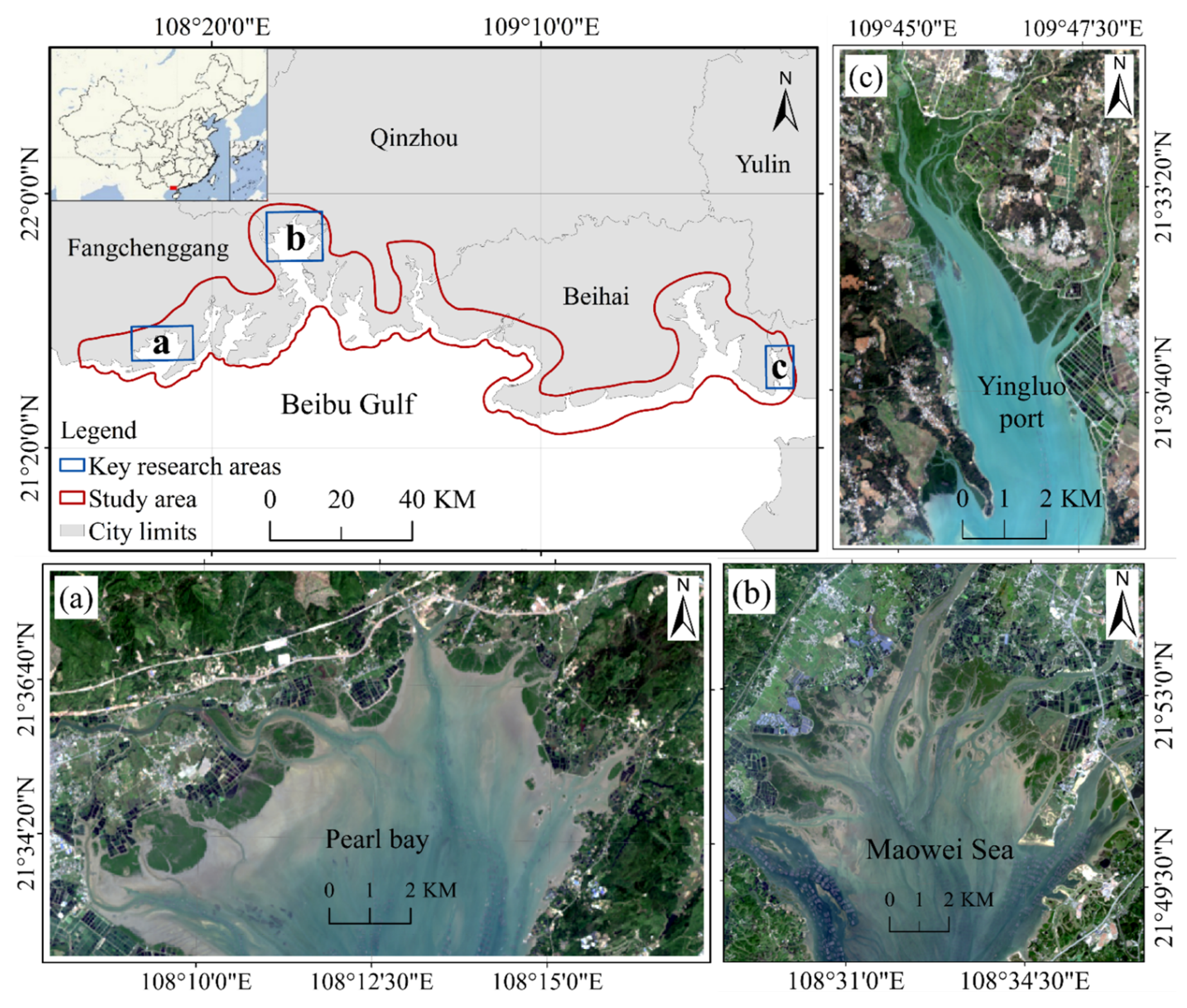
2.1. Study Area

The study area is located in the Guangxi coastal zone of Beibu Gulf in China (Long. from 21°24′20″N to 22°01′20″N, Lat. from 107°56′30″E to 109°40′00″E). The study area is a typical distribution of tidal flats and mangroves with abundant ecological resources [29,30,31]. The area covers the southwest end of mainland China, close to the Leizhou Peninsula in the east and Vietnam in the west, and has a total length of approximately 1600 km [31]. The Beilun, Fangcheng, Maoling, Qinjiang, and other rivers flow into the Beibu Gulf (Figure 1). Mangroves are widely distributed in the study area and are the dominant vegetation of coastal tidal flats in China (Figure 1).

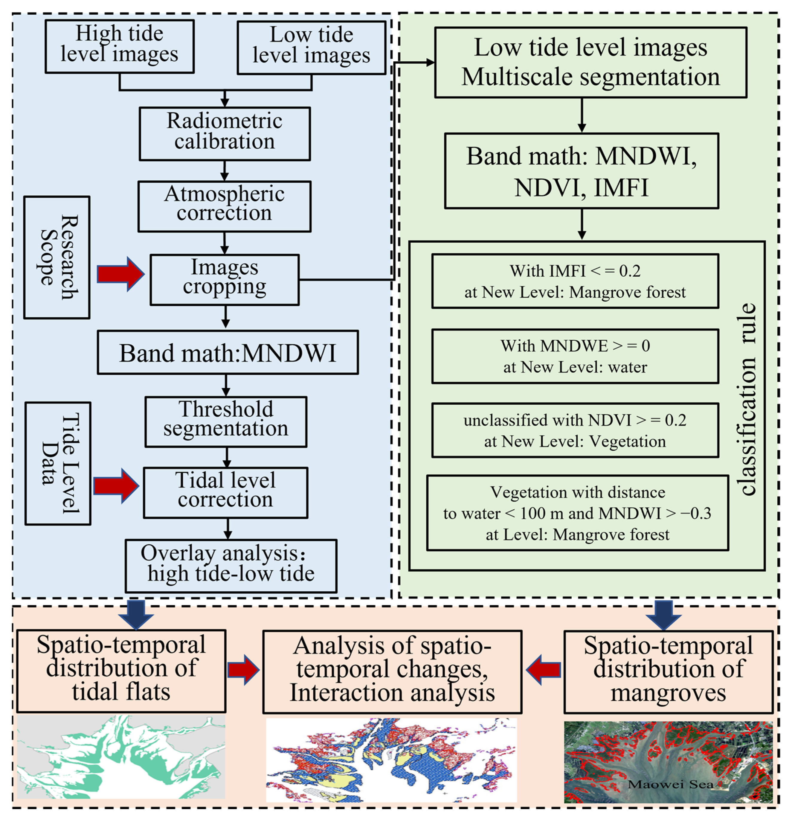
2.2. Data Acquisition and Pre-Processing

In this study, Landsat 5-TM imageries, Landsat 7-ETM+, Landsat 8-OLI, Landsat 9-OLI2 imageries were downloaded from China’s Geospatial Data Cloud (GSCloud, www.gscloud.cn) and United States Geological Survey (USGS, earthexplorer.usgs.gov) accessed on 5 January 2022 and 9 January 2022, respectively, and Sentinel-2 imageries were downloaded from the European Space Agency (ESA, scihub.copernicus.eu (accessed on 1 February 2022)). A total of 148 images from various sensors covering the study area with a cloud cover of less than 10% were selected (Table 1), covering the period from 1987 to 2021. To ensure that the images covered the entire study area, two Landsat series images and four Sentinel-2 images were selected for stitching. As the images were acquired at different time periods, it was necessary to conduct a tide-level correction and then merge [32,33]. The Raster Processing Batch Tool of ENVI 5.6 software was used for radiometric calibration, atmospheric correction, and image cropping. For radiation calibration, the “Radiometric Calibration Batch” tool was used to batch process Landsat series images. The radiation calibration parameter settings are as follows: Set the calibration type to radiance data, set the storage format to BIL, output a single precision floating point data type, and fix the adjustment coefficient to 0.1 [34]. Atmospheric correction uses the “QUAC Batch” tool to process radiometric calibrated images, allowing for the quick batch processing of images from the same sensor by simply setting the sensor type. The Sen2Cor plug-in released by the ESA was used to preprocess the Sentinel-2 image L1C product data [31].
The daily maximum and minimum tide levels at the three tide gauge stations at Fangcheng Harbor, Longmen Harbor, and Beihai Harbor from 1987 to 2021 were obtained from the China Ocean Information Center (http://globaltide.nmdis.org.cn/ (accessed on 7 January 2022)) [35], and the annual average high- and low-tide levels at the three tide gauge stations were calculated.

2.3. Extraction of Tidal Flats

The range of tidal flats to be extracted in this study was the tidal intrusion zone between the annual mean high- and low-tide levels [36]. The major steps included:

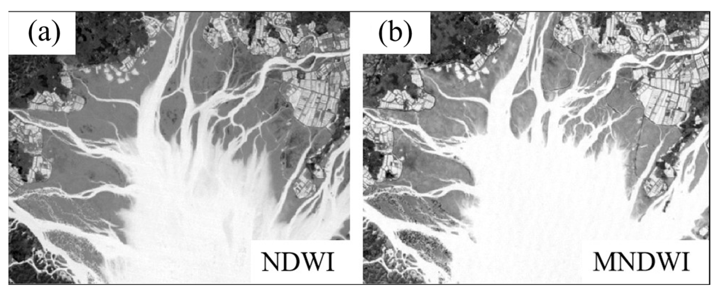
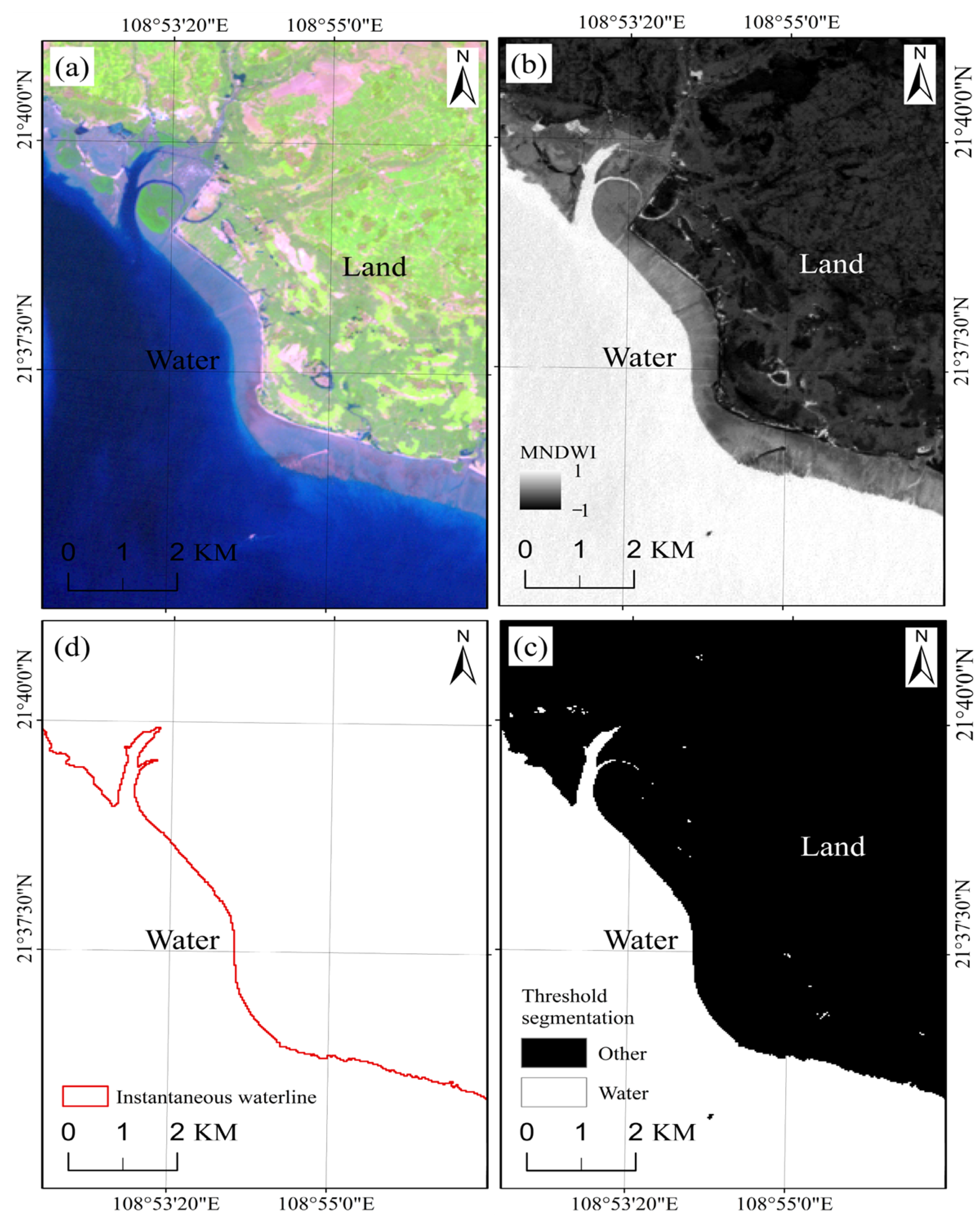
2.3.1. Instantaneous Water-Edge Line Extraction

Traditional methods were applied to remotely sensed images with bands of 0.4−2.5 μm to identify the water bodies, but it is difficult to identify the water-edge line accurately due to the influence of water depth, suspended matter, and impurities [37,38]. This study proposes a combination of multiband differences or ratios [7], including the normalized difference water index (NDWI) and modified normalized difference water index (MNDWI) [1,2].
N D W I = ( R G reen - R N I R ) ( R G reen + R N I R )
M N D W I = ( R G reen - R S W I R 1 ) ( R G reen + R S W I R 1 )
where RGreen is the green band reflectance, RNIR is the reflectance of the near-infrared band, and RSWIR1 is the reflectance of the mid-infrared band.
As shown in Figure 2, the MNDWI can suppress the influence of suspended sediment in water and prevent their identification as shoals. The experimental results demonstrated that the proposed method can effectively extract water bodies’ information containing a small number of fragmented patches and more accurately extract the instantaneous water-edge line represented by remote sensing images. Therefore, this study adopted the threshold segmentation method, setting the segmentation threshold based on the MNDWI index, retrieving all pixels in the image according to the set threshold [24], and dividing them into water and non-water categories. Owing to the different image acquisition times, it was difficult to use a fixed threshold to distinguish all water and non-water images. In this paper, we first counted the boundary thresholds of multiple images and their range from 0 to 0.1, and then applied this threshold range to all images. After threshold segmentation, the image was binarized, and the vector graphics derived. The results are shown in Figure 3.

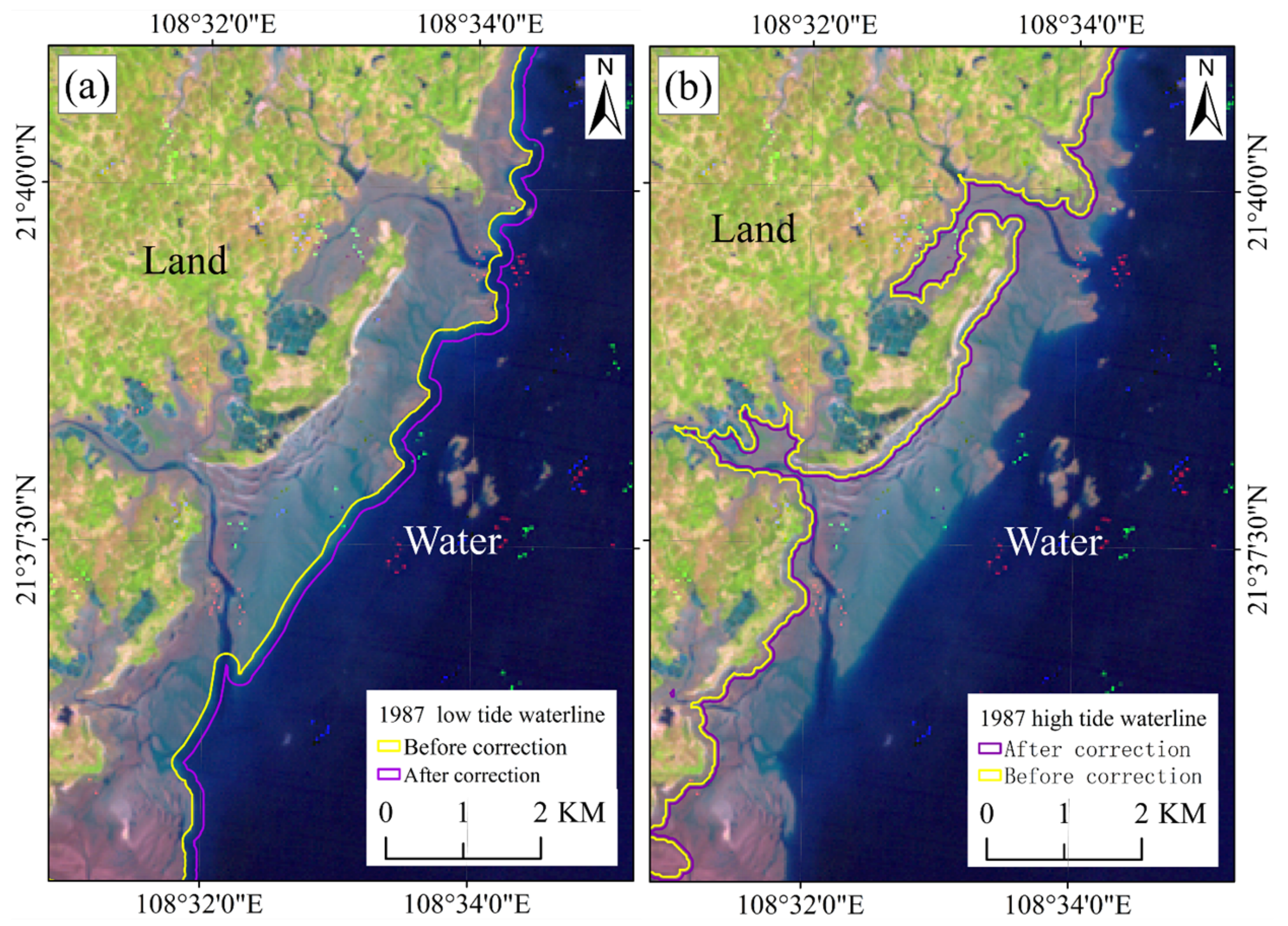
2.3.2. Tidal-Level Correction

The extent of exposure to tidal flats depends heavily on tidal height. Moreover, the instantaneous water-edge line extracted using a single time phase cannot represent the true land–sea interface [39]. Therefore, it is necessary to define the range of tidal flats at a unified scale to study their sequential changes. The instantaneous water-edge line was corrected to the annual high- and low-tide lines [40,41,42], as shown in Figure 4 [43,44].
In this study, two instantaneous waterside lines were extracted using two remote sensing images acquired at similar times, and several points were considered from two adjacent waterside lines at a certain distance. The distance between the adjacent points depended on the straightness of the coastline, and was reduced if the coastline was curved. The average distance between the two waterside lines was determined using corresponding points on the two waterside lines, and the slope of the tidal flats was calculated based on the difference in the tidal level of the two waterside lines. Finally, the instantaneous water-edge line was corrected to the annual mean spring-, high-tide line or annual mean neap-, low-tide line based on the tidal flats’ slope and tide-level data at the moment of image acquisition [45,46].
Where Hhigh is the annual mean high-water spring tide; Hlow is the annual mean low-water neap tide; h1 is the instantaneous tide height at the moment of high-tide image acquisition; h2 is the instantaneous tide height at the moment of low-tide image acquisition; ΔH is the tidal-level difference at the time of high-tide and low-tide image acquisition; ΔL is the distance between the instantaneous high-tide water edge and the instantaneous low-tide water edge; θ is the slope of tidal flats; Lhigh and Llow are the correction distances for the tide level. Different parameters were calculated using the following equations:
Δ H = h 1 h 2
θ = arctan Δ H Δ L
L l o w = h 2 H l o w tan θ
L h i g h = H h i g h h 2 tan θ
As shown in Equations (5) and (6), to obtain the high- and low-tide correction distances Lhigh and Llow, it is necessary to calculate the instantaneous tide height at the moment of high-tide and low-tide image acquisition h1 and h2. The tide-level data could only be obtained from the China Marine Information Center for the entire point and peak of the day. However, the tidal change within a day was an approximate trigonometric curve, and the tidal change between adjacent points could be estimated as a linear relationship. Therefore, the height of the tidal level at a certain time was calculated using Equation (7).
h = h l e f t + ( h l e f t h r i g h t ) T h T l e f t T r i g h T l e f t
where h is the instantaneous tide height at the time of image acquisition, hleft is the instantaneous tide height at one full point before the image acquisition time, hright is the instantaneous tide height at one full point after the image acquisition time, Th is the time of image acquisition, Tleft is the time before the image acquisition time, and Tright is the time after the image acquisition time. Tleft and Tright could be extrapolated from Th, the corresponding hleft and hright could be queried, and then Equation (7) could be interpolated to calculate h1 and h2. Substituting h1 and h2 in Equations (3)–(6), the correction distance was obtained using Lhigh and Llow. Based on the tidal correction distances Lhigh and Llow, a tidal correction was applied to the extracted instantaneous water-edge line, where positive values indicated seaward extension and negative values indicated shoreward movement. Figure 5 shows a comparison before and after correction of the local water-edge line. In 1987, the low-tide water-edge line extended 146 m into the sea, whereas the high-tide water-edge line extended 68 m into the sea. The range of tidal flats can be obtained using a superposition analysis of high-tide and low-tide water-edge lines after the completion of tidal-level correction.

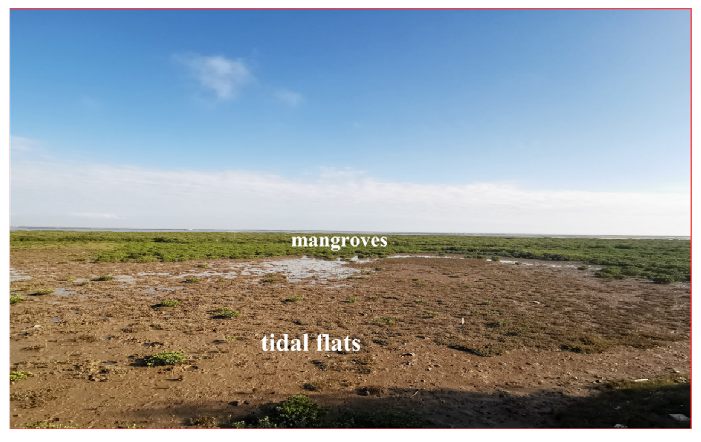
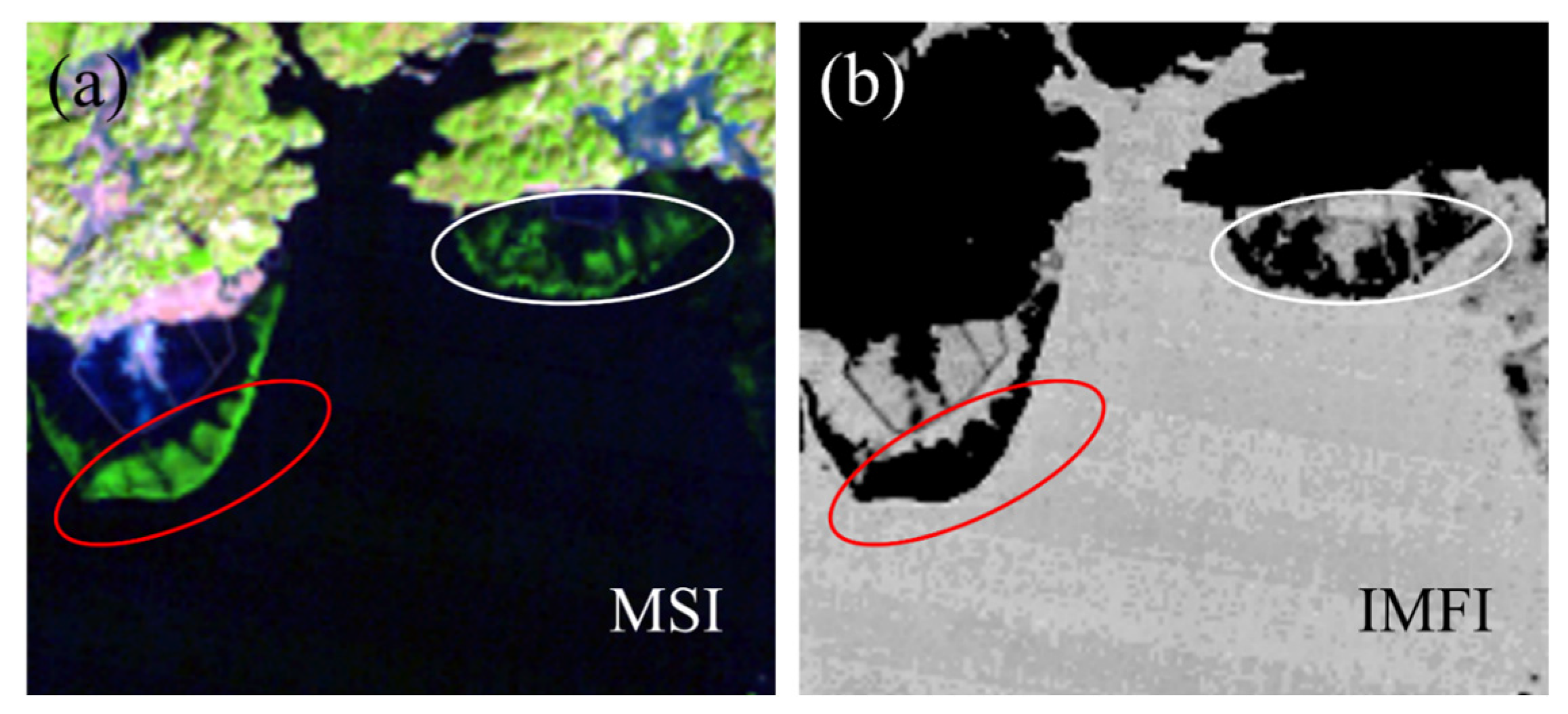
2.3.3. Spatial Distribution of Mangroves in Tidal Flats

Mangrove forests can reduce the velocity of seawater, facilitate sediment deposition, and accelerate the development of tidal flats (Figure 6) [47,48,49,50]. To quantitatively investigate the role that spatio-temporal changes in mangroves play in the spatio-temporal changes in tidal flats, this study used an object-oriented multiscale segmentation method based on eCognition 10.2 software to remotely identify and extract the main mangrove distributions in the study area [51,52]. In this study, the segmentation scale was determined to be 200, and the shape factor and compactness were set as 0.2 and 0.5, respectively. Image elements of remote sensing images were no longer the smallest unit of classification after multiscale segmentation, and image objects replaced the spectral, shape, texture, and spatial relationship features among the image objects.
To accurately extract the required object information, the MNDWI, normalized difference vegetation index (NDVI), inundated mangrove forest index (IMFI) [53], and the spatial relationship feature of distance from mangroves to water bodies were selected to build the rule tree in this study. NDVI was calculated using Equation (8). It ranges from −1 to 1 and is often used to distinguish between vegetation and non-vegetation.
N D V I = ( R N I R R R ) ( R N I R + R R )
where RNIR is the reflectance of the near-infrared band and RR is the reflectance of the visible red band.
The IMFI calculated using Equation (9) was used to extract a small number of mangroves inundated by the tide at low tide [53]. This index can distinguish between the inundation of mangroves and tides by combining the characteristics of visible blue wave segments with strong water penetration ability, and visible green and near-infrared bands with extreme sensitivity to green plants.
I M F I = ( R b l u e + R g r e e n 2 R n i r ) ( R b l u e + R green + 2 R n i r )
where Rblue is the visible blue band reflectance, Rgreen is the visible green band reflectance, and Rnir is the NIR band reflectance.
Figure 7a,b shows the multispectral imagery and IMFI imagery, respectively. The figure shows that the IMFI index can enhance the display of mangroves in the seawater inundation area. In the IMFI imagery, the overall brightness of the mangrove is lower than that of the surrounding seawater, and the outline of the mangrove is clearly visible. This shows that IMFI has the ability to differentiate between inundated mangroves and seawater.
After several experiments, the following classification rules were developed: ① Objects with IMFI ≤ 0.2 were classified as mangroves, and objects with MNDWI ≥ 0 as water bodies; ② objects with NDVI ≥ 0.2 were classified as vegetation in the unclassified objects; ③ in vegetation classification, objects with MNDWI > −0.3 and less than 100 m away from the water bodies were classified as mangroves to realize the time sequence extraction of mangroves in the study area.
In summary, the technical route of this paper is shown in Figure 8.

3. Results and Discussion

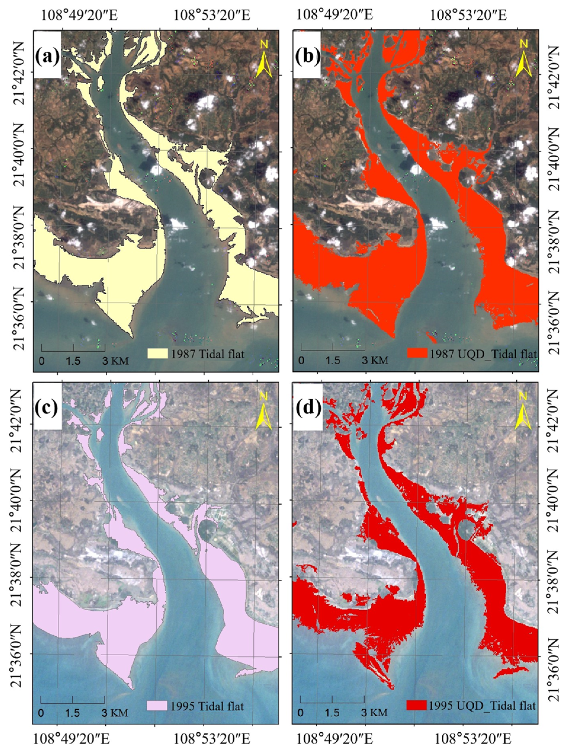
3.1. Reliability Analysis of Tidal Flat Extraction Results

In this study, a confusion matrix was used to analyze the accuracy of the obtained tidal flats, and random points were generated on the edges of the high- and low-tide lines without tidal-level correction. The confusion matrix was calculated for every year for 35 years through a visual interpretation of the land class, and the overall accuracy and kappa coefficient were used to evaluate the classification accuracy (see Table 2 and Table 3). As shown in Table 2 and Table 3, the overall accuracy of the annually extracted tidal flats was greater than 90%, and the kappa coefficient was greater than 0.75. Moreover, the kappa coefficient of the tidal flats’ extraction results for 27 years was greater than 0.8, accounting for approximately 77% of the tidal flats’ extraction results. The combined 35 years of extraction results showed an overall accuracy of 93.9%, a kappa coefficient of 0.82, and a user accuracy and mapping accuracy of >85% for tidal flats. The confusion matrix showed that the extent of the tidal flats extracted based on spectral index threshold segmentation was highly consistent with the visually interpreted ground types, and the extraction results were reliable.
In addition, this study compared the accuracy of the tidal flats dataset UQD (University of Queensland global tidal flats dataset) produced by Murray et al. from the University of Queensland during 1986−2016 to analyze the tidal flats’ extraction results of each bank segment of Beibu Gulf [6]. The UQD is a global tidal flats dataset obtained based on the random forest algorithm and a large number of training samples; however, some inland wastelands, aquaculture ponds, and intertidal salt marshes in the UQD are included in the tidal flats range [7]. Figure 9 shows a comparison between the tidal flats range of the Beihai section extracted in this study (Figure 9a,c) and the UQD data (Figure 9b,d). The UQD is shown to be consistent with the extraction range of this study. However, a small trench is slightly different, and part of the inland soil in the UQD was misclassified as tidal flats.
In summary, the tidal flats’ extraction method using threshold segmentation and tidal-level correction can obtain a wide range of tidal flat distributions, and the obtained results have high accuracy and a wide range. The method can be used for large-scale tidal flats’ extraction, long-distance shoreline extraction, and coastal zone wetland classification.

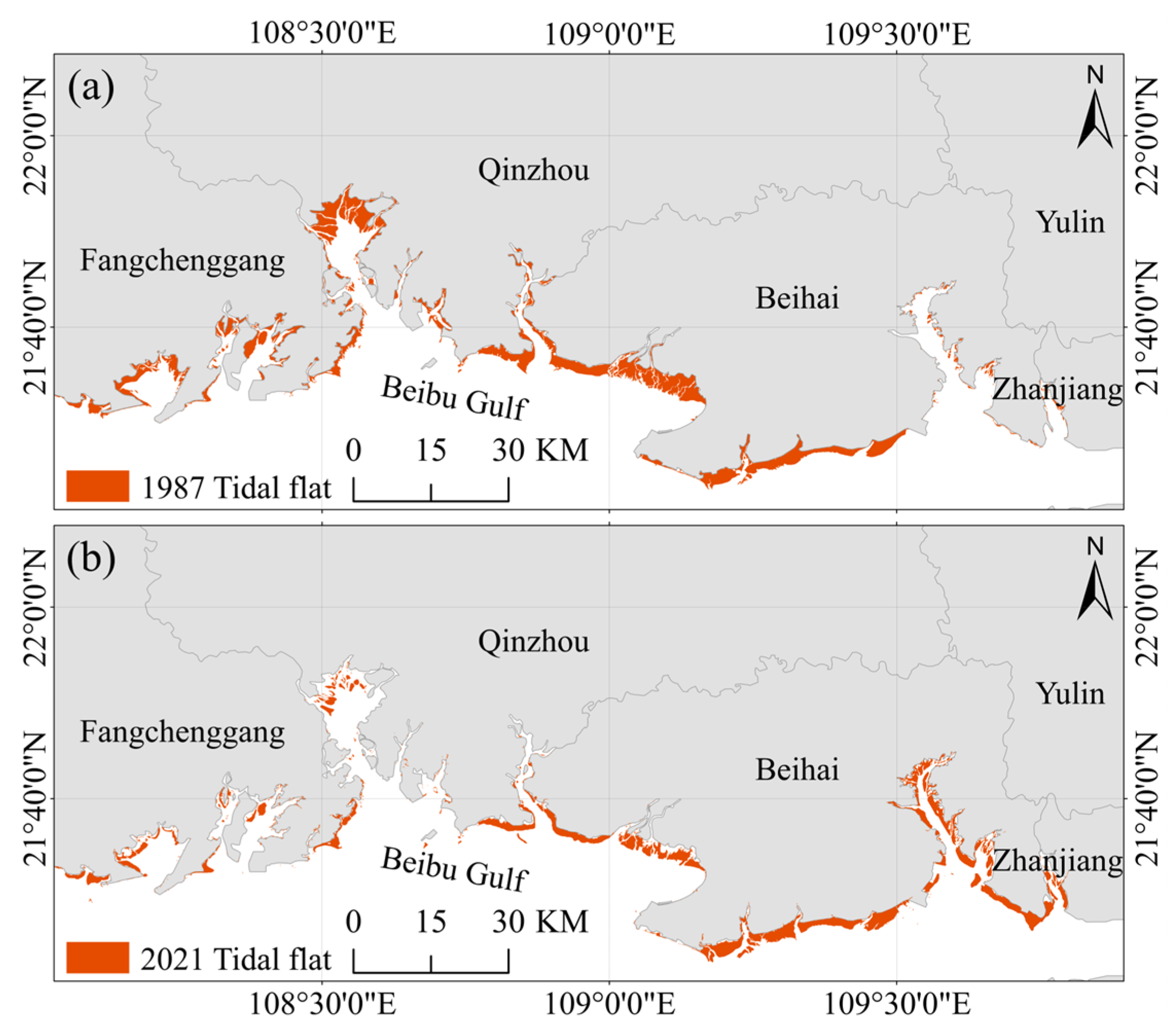
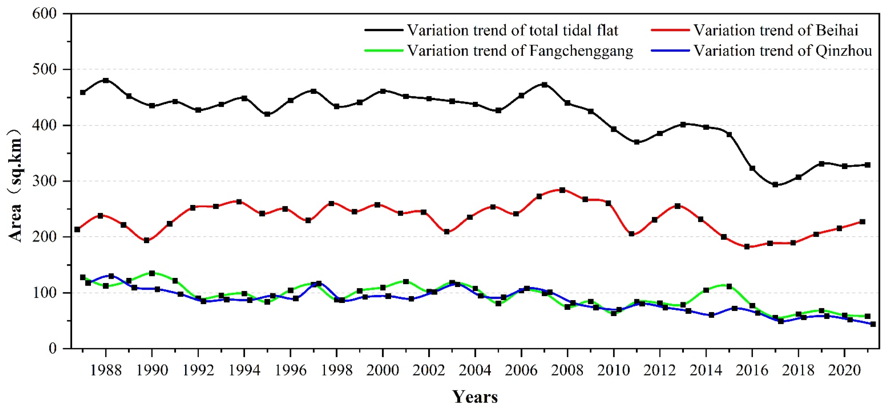
3.2. Spatio-Temporal Variation of Tidal Flats in Beibu Gulf

The distribution of tidal flats in the Beibu Gulf of Guangxi in 1987 and 2021 is shown in Figure 10, and the temporal variation in the total tidal flats and tidal flats in each bank segment from 1987 to 2021 are shown in Figure 11. The total tidal flat area decreased from 458.9 km2 in 1987 to 328.9 km2 in 2021, with a decrease of 28.3% and an average annual change of −3.7 km2/a. The tidal flat area gradually changed from 1987 to 2005; from 1992 to 2000, it increased and decreased regularly within a three-year cycle, and fluctuated between 420 km2 and 460 km2. Since 2001, the overall tidal flat area of the study area decreased. From 2007 to 2011, the tidal flat area continued to decrease at a rapid rate, with the total area decreasing to 102.3 km2 at the rate of −25.6 km2/a. The tidal flat area slightly increased from 2011 to 2013, and then continued to decrease until 2018. Over the 35 years, the largest tidal flat area was 480.2 km2 in 1988, followed by 472 km2 in 2007. In 2017, the tidal flat area was the smallest at 293.7 km2. Overall, the total tidal flat area in the study area continuously decreased from 1987 to 2021.
Due to the large east–west span of the study area and obvious tidal differences, the study area was divided from west to east into three sections according to administrative regions: the Fangchenggang bank section from Beilun Estuary to the west coast of Qinzhou Bay; the west coast of Qinzhou Bay to the south Qinzhou bank section of the Fengjiang River; and the Beihai section from the south of the Fengjiang River to Yingluo Port.
The tidal flat area in the Beihai section slightly increased between 1987 and 1993. The trend from 1994 to 2008 was moderate, with little change in the overall stock. From 2003 to 2005 and 2006 to 2008, there were short periods of continuous slow growth, by areas of 44.1 km2 and 42.2 km2, respectively. This increase in area was primarily due to tidal siltation, with a decrease over the remaining years. From 2003 to 2005, the main silting coasts were Tieshan Port and Yingluo Port. From 2006 to 2008, the main silted coast extended from Lianzhou Bay to Beiwu Salt Farm (Figure 12). In 2008, the tidal flat area of the northern coastal section reached 283.8 km2, accounting for 64.5% of the total tidal flat area of Beibu Gulf in Guangxi. From 2008 to 2018, the tidal area gradually decreased to 189.7 km2, at a rate of −9.4 km2/a and an amplitude of 93.6 km2. The primary reason for this decrease was tidal erosion, which was distributed along the coast from Lian Zhou Bay to Bailong Port. From 2019 to 2021, the tidal flats area of the Beihai section slowly increased, and the tidal flats stock in 2021 was 227.4 km2.
The maximum tidal flat area of Qinzhou shore was 129.9 km2 in 1988 and the minimum tidal flat area was 43.6 km2 in 2021, with an area variation of 86.3 km2 over 35 years, as shown in Figure 13. From 1987 to 1993, a slow reduction interval occurred, with a reduction rate of 29.9 km2 at approximately −3 km2/a. The main reduction shores were the southern shoreline of the outlet of the Dafeng River, the northwestern shoreline of Xiniujiao Town, and the northern near-shore shallow area of the Maowei Sea. The overall stock of tidal flats was stable from 1993 to 2007, and increased by 29 km2 from 1993 to 1997. The primary reason for the increase in area was the siltation of the tidal flats near the shallow Maowei Sea and along the southern coast of the Dafeng River outlet. A decrease of 20.9 km2 occurred from 1997 to 1998, and the main erosional area was shallow along the northern coast of the Maowei Sea. From 1999 to 2007, the siltation erosion area and regional distribution were consistent with the changes during this period. From 2008 to 2021, the tidal flat area shows an obvious decreasing trend, which is consistent with the changing trend of the total tidal flat area in Guangxi. In the past 13 years, the tidal flat area decreased by 38.3 km2, with a reduction rate of about −3 km2/a. The main cause of the tidal flats erosion was the reclamation of coastal tidal flats north of the Maowei Sea for aquaculture.
The maximum tidal area of the Fangchenggang shore section was 134.9 km2 in 1990, and the minimum was 55.8 km2 in 2017. In the past 35 years, the area change range reached 79.1 km2, with an average annual change rate of −3 km2/a. The chronological changes are shown in Figure 14. From 1987 to 1993, the total area decreased by 32.7 km2, first increasing, and then rapidly decreasing. The eroded area is evenly distributed throughout the shore section of Fangchenggang, except on the artificial coast. The period from 1995 to 2005 was stable: the regularity fluctuated and the tidal flats stock tended to be stable. From 2008 to 2017, the tidal flat area initially increased and then decreased, peaking in 2015. It increased slowly in the early period and decreased rapidly in the late period, which differed from the tidal flat areas of the other two bank segments and the total tidal flat area in Guangxi. Among them, the tidal flat area increased by 36.8 km2 from 2008 to 2015, accounting for 49% of the tidal flat area of Fangchenggang in 2008, with a change rate of 7 km2/a. The largest increase and rate of the tidal flats siltation area occurred over 35 years, with the main siltation areas being the Beilun Estuary, Pearl Bay coast, and the western coast of Qinzhou Bay. In the period 2015−2017, the tidal flat area decreased by 55.5 km2, and the tidal flats along each bay were largely eroded.

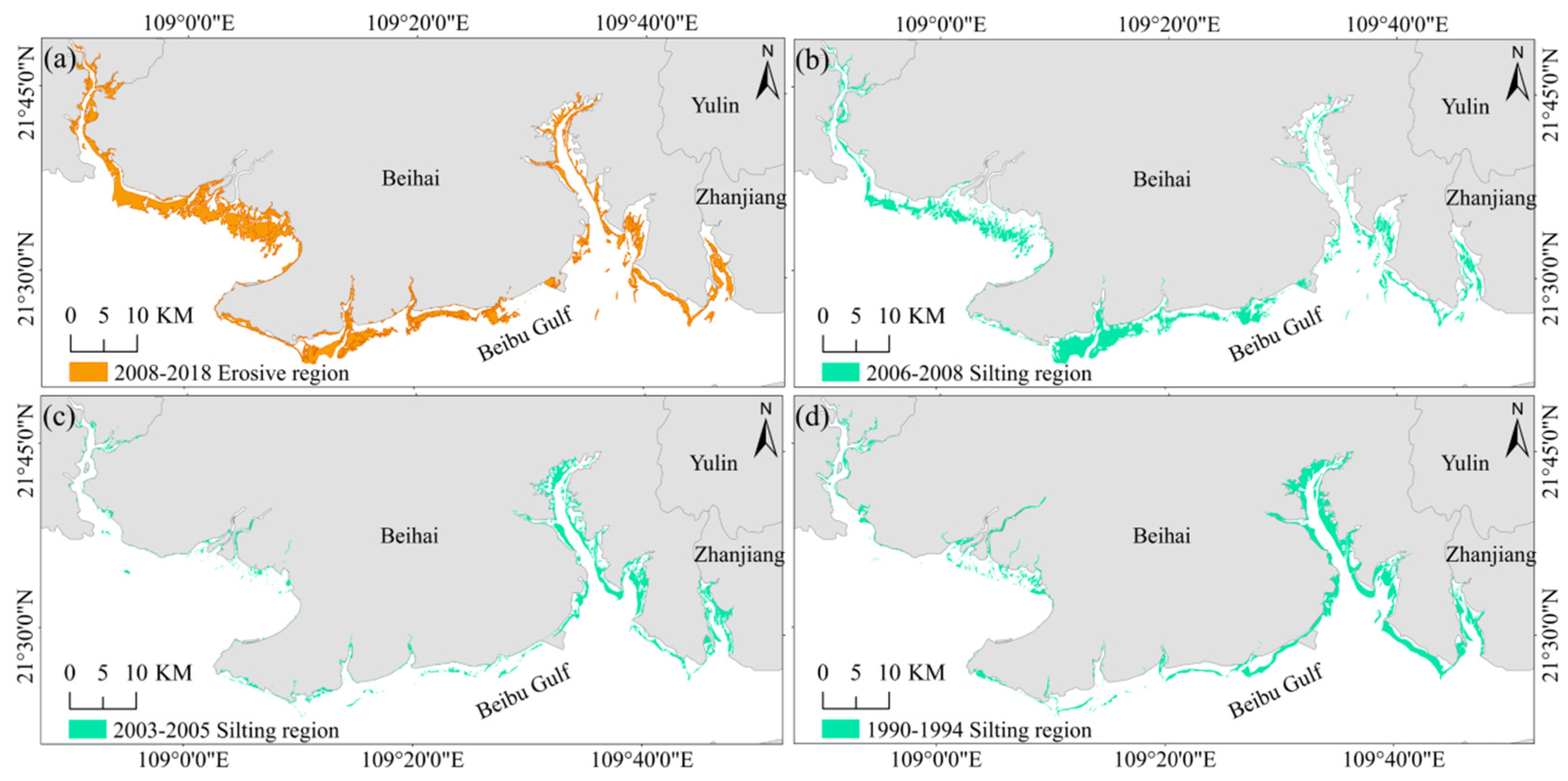
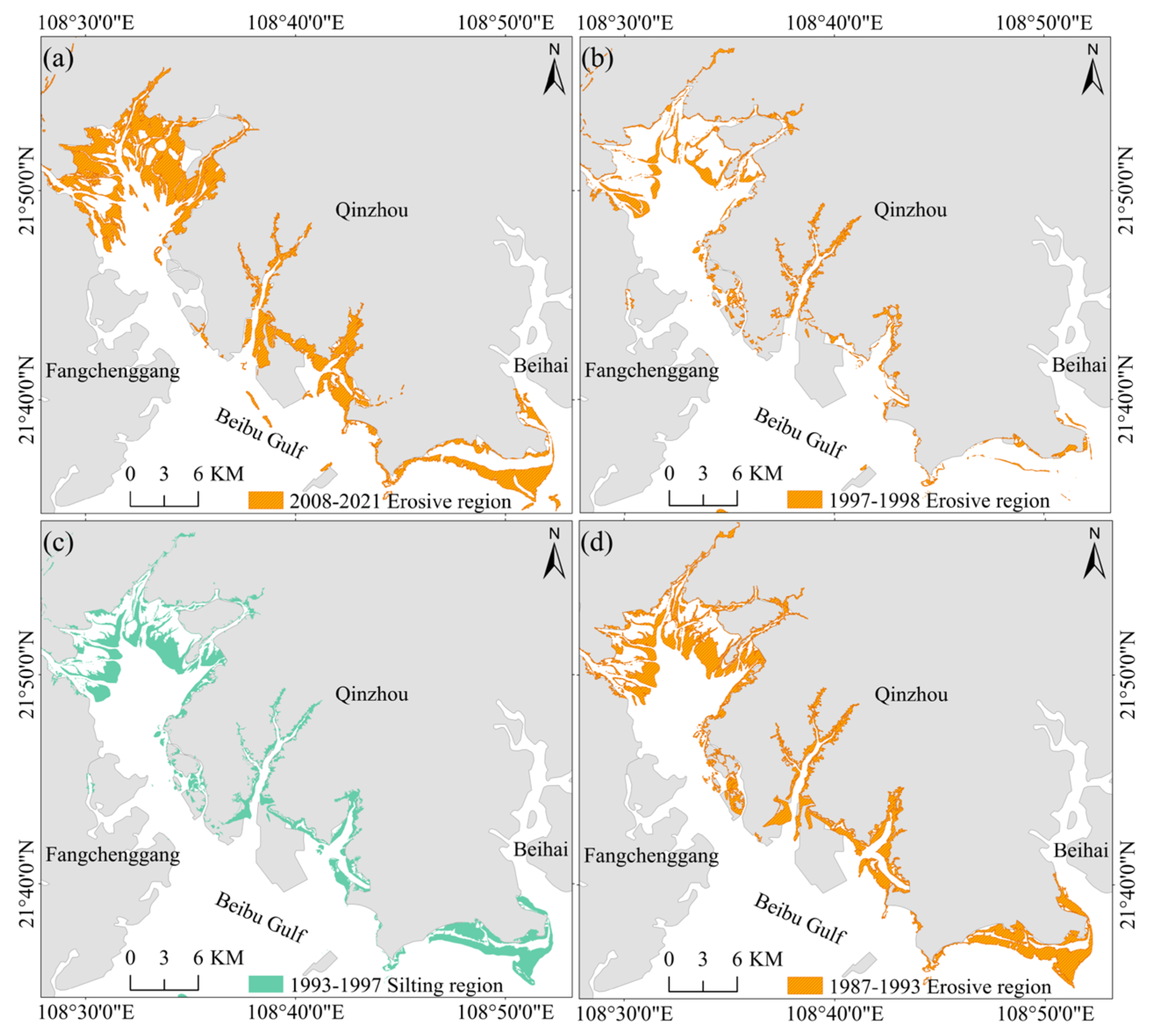
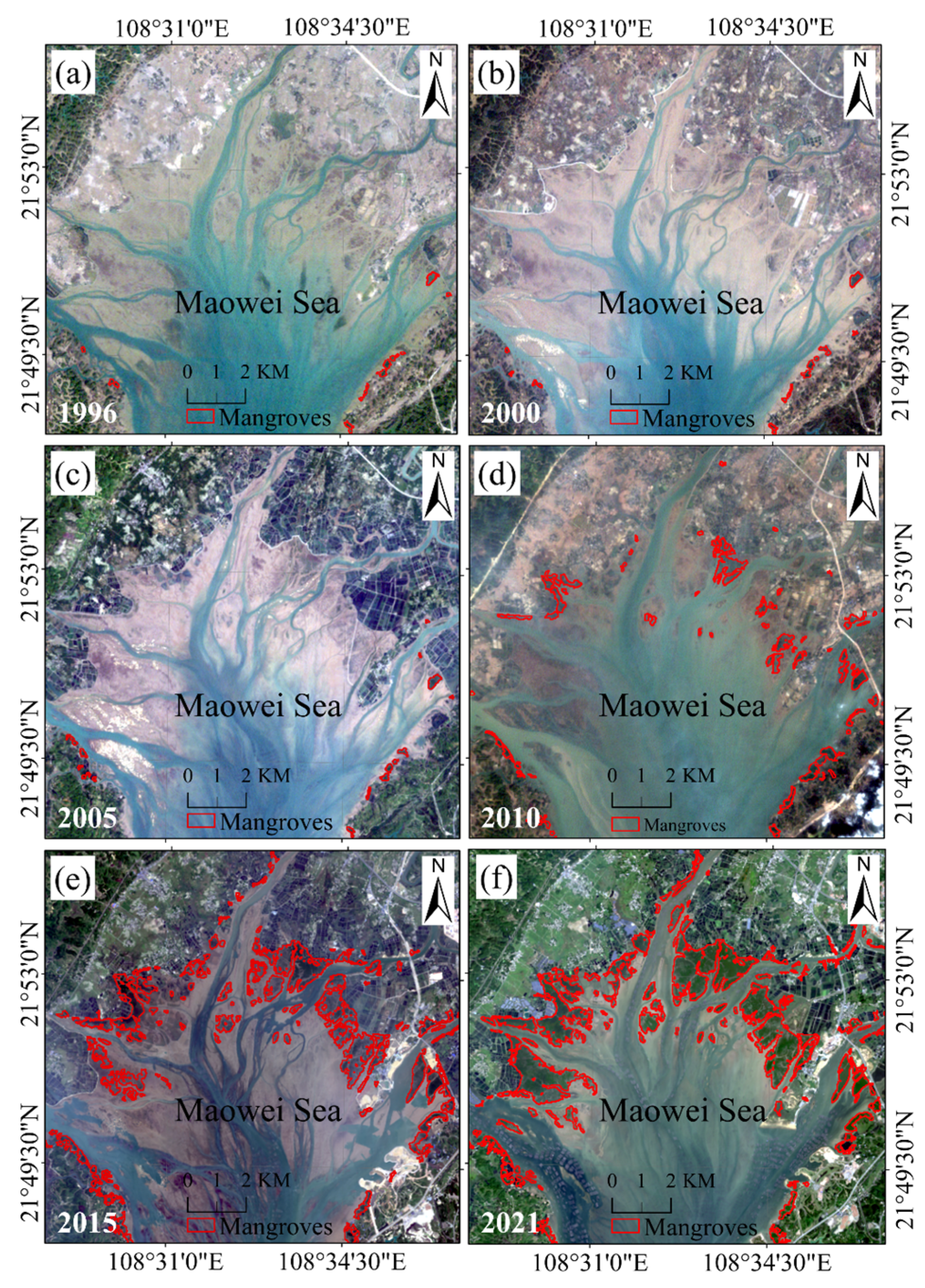
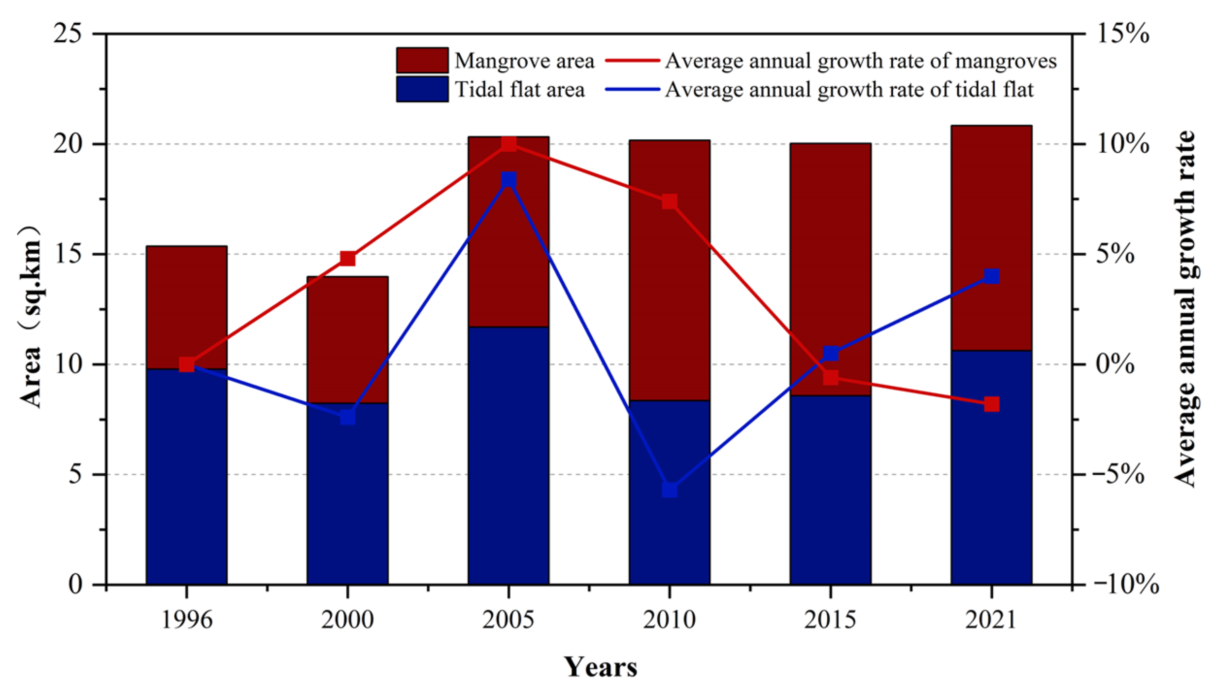
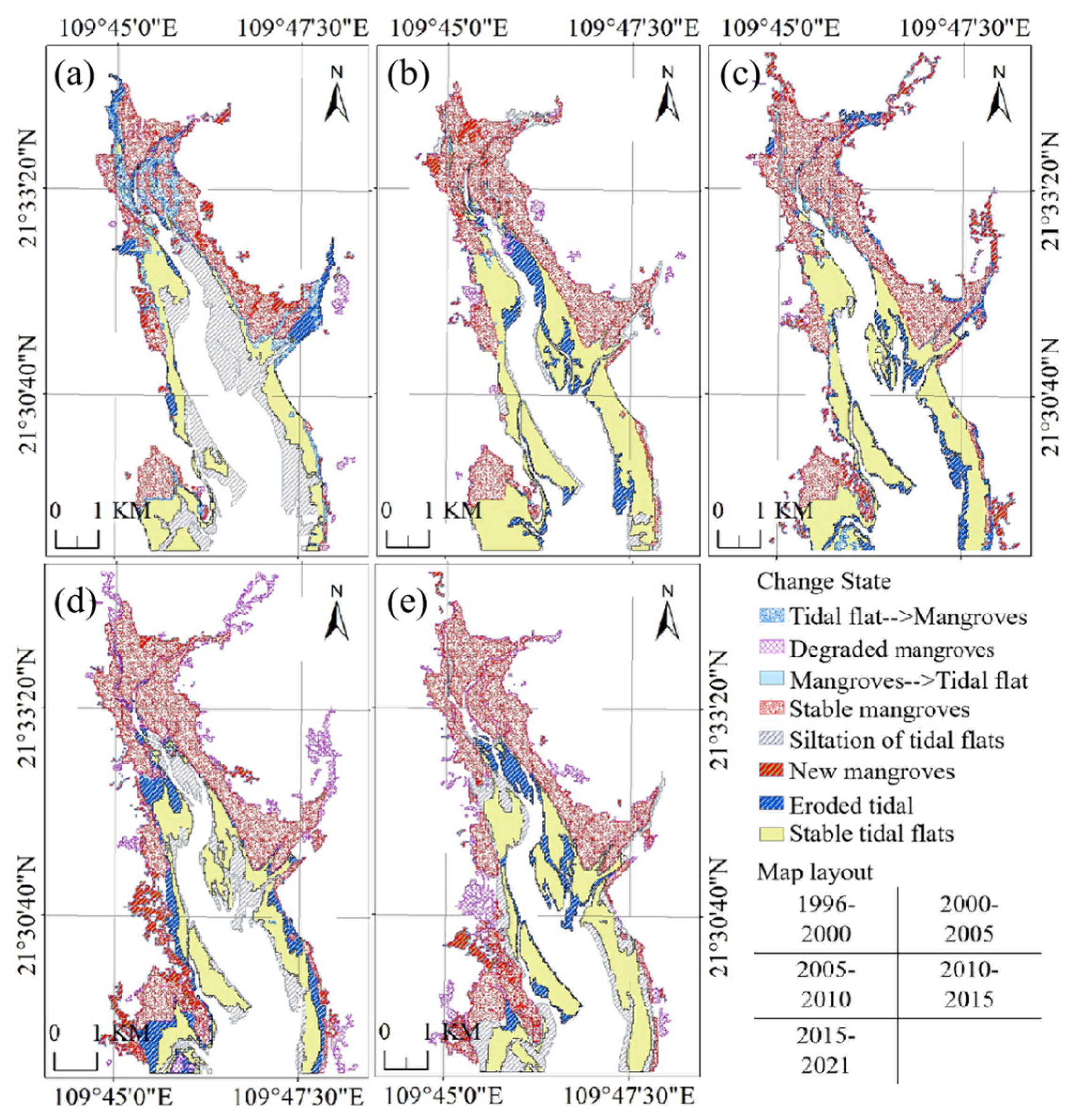
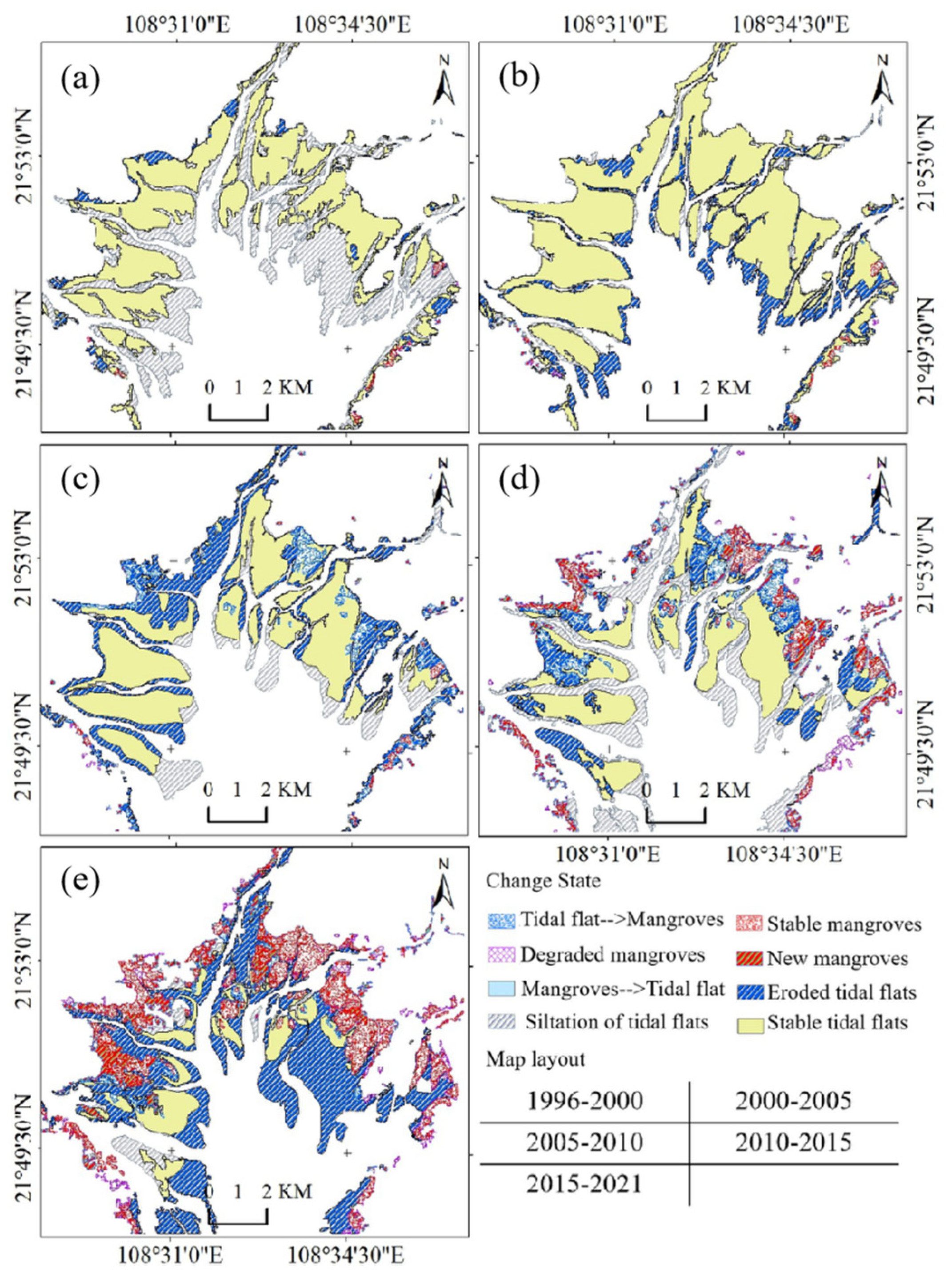
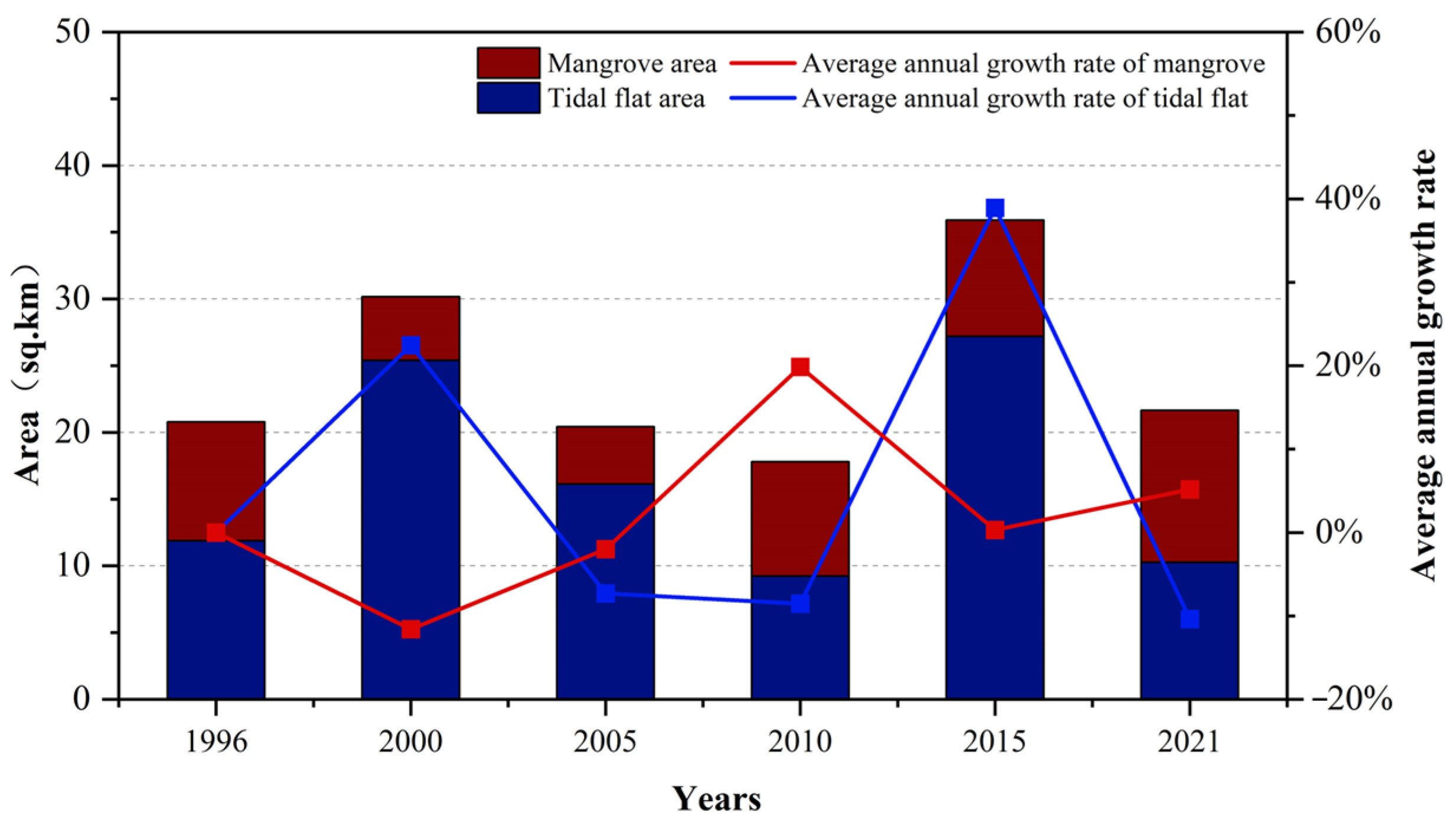
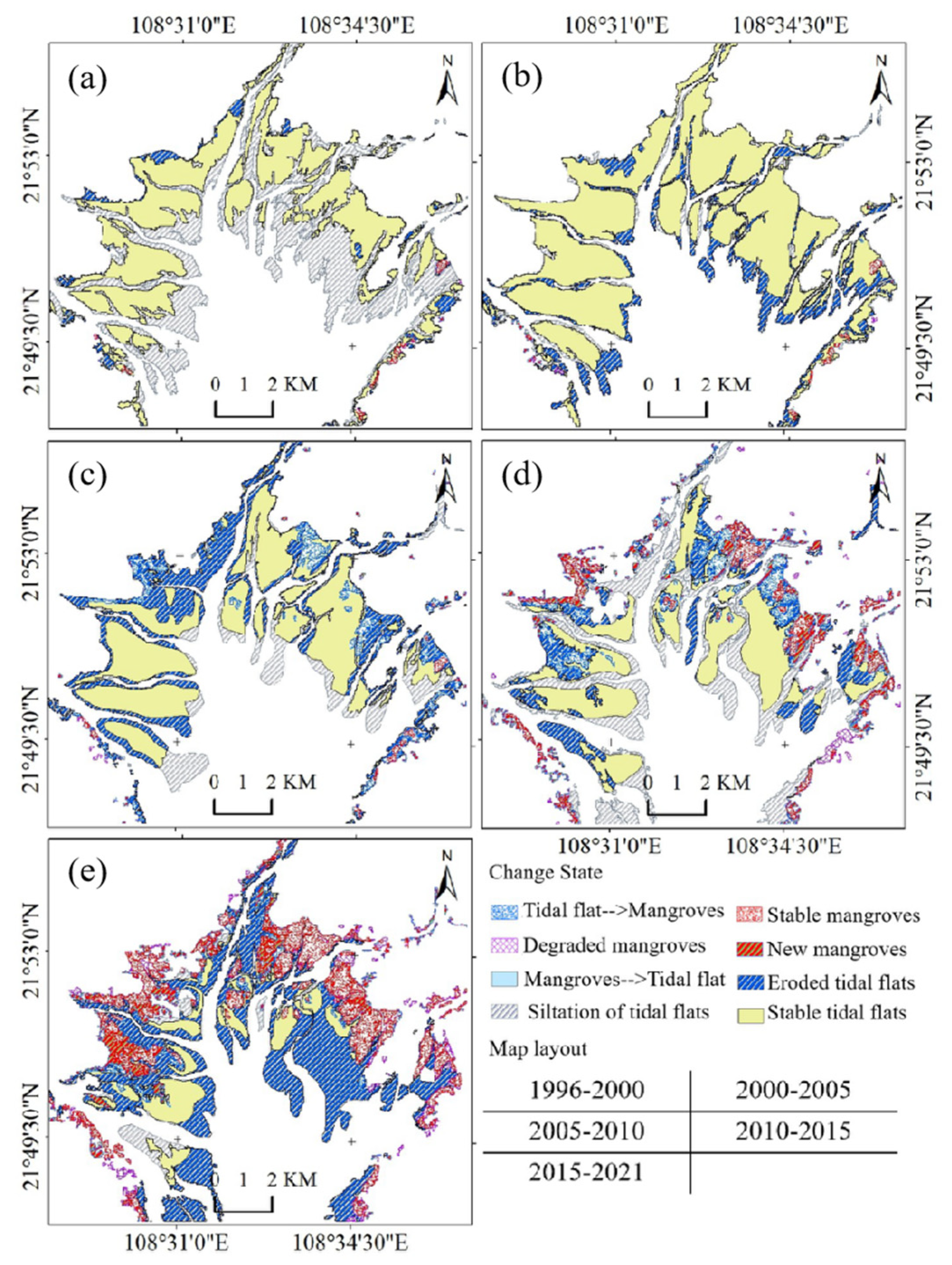
3.3. Analysis of Spatio-Temporal Changes in Tidal Flats as Influenced by Temporal Changes in Mangrove Forests

The mangroves in the study area were concentrated in three areas namely, Shankou, Maowei Sea, and Pearl Bay. As the mangrove area in the study area was very small before 1996 and the magnitude of change was small, the time-series distribution of mangroves in the three areas from 1996 to 2021 was extracted in this study. Considering the Maowei Sea Mangrove Reserve as a case study, Figure 15 shows the time-series changes in the distribution range of mangrove vegetation in the Maowei Sea over a 25-year period, suggesting that the area of mangroves continues to grow rapidly. Time-series changes in mangrove areas are shown in Table 4.
The distribution of tidal flats and mangroves in the study area in 2021 is shown in Figure 16. The mangrove stock in the three mangrove concentration areas showed an increasing trend, except for the years 1996−2000, when the total stock was negative. The remaining years showed a positive growth, with a maximum annual average growth rate of 16.6% in 2010. However, the total tidal flats in the three mangrove areas showed a decreasing trend, with a maximum negative annual growth rate of −9.1% in 2021 and a total decrease of 21 km2 in tidal flats over the 25-year period.
The stock and annual growth rates of tidal flats and mangroves in the Shankou area from 1996 to 2021 are shown in Figure 17. The mangrove stock generally showed an increasing trend, with a continuous increase from 1996 to 2010 and an average annual growth rate of 10% from 2000 to 2010. The highest average annual growth rate was observed for many years. In 2021, the total mangrove stock increased by 4.63 km2 compared with 1996, with a cumulative growth rate of 83%. The overall trend of tidal flats stock was stable, with a dynamic balance of growth followed by a decline, in which the average annual growth rate reached 8.4% during 2000−2005 and −5.7% during 2005−2010. The correlation coefficient r between the change in tidal flats stock and the change in mangrove stock was −0.28; that is, the growth of tidal flat areas and mangrove areas showed a weak negative correlation. The temporal changes in tidal flats and mangroves for each of the five years are shown in Figure 18. Analysis of the temporal changes in tidal flats and mangroves between the study areas showed that the natural growth in mangroves in Shankou was mainly distributed along the northern coast of Yingluo Bay during 1996–2005, the eastern coastal Cape during 2005, and the western coast during 2010–2021. Mangrove degradation was mainly distributed along the eastern Cape of Yingluo Bay from 1996 to 2000, several capes along the eastern coast from 2010 to 2015, and the eastern coast from 2015 to 2021. However, the distribution of the tidal flats was relatively stable, and there was no large-scale disappearance of the tidal flats.
A one-dimensional cubic polynomial regression model was developed based on the changes in the mangrove and tidal flat areas. The coefficient of determination R2 of the regression model was calculated as 0.88 for the study area of Yingluo Bay. This suggested that the relationship between mangroves and tidal flats that increased and decreased in the Shankou Mangrove Nature Reserve from 1996 to 2021 had a high fit with this regression model. The relationship between changes in mangrove and tidal flat areas was assessed based on a high-fit model.
The stock and average annual growth rates of land types (tidal flats and mangroves) in the Maowei Sea region from 1996–2021 are shown in Figure 19. Mangrove stocks showed a growing trend, with a continuous increase from 1996 to 2021 and an average annual growth rate of 145% from 2005 to 2010. The largest average annual growth rate over many years was mainly due to the small base of mangrove stocks in the previous period, which caused a dramatic increase in the rate of change with even a slight increase in area. In 2021, compared with 1996, the total number of mangroves increased by 18.09 km2. The tidal flats stock generally exhibited a decreasing trend, with the interval showing an increase followed by a decrease. The average annual growth rate was 17.1% from 1996 to 2000 and −11.3% from 2015 to 2021. The correlation coefficient r between the change in tidal flats stock and the change in mangrove stock was −0.30, and the growth in tidal beach area was negatively correlated with the growth in mangrove area.
As shown in Figure 20, the growth area of mangroves in the Maowei Sea from 2005 to 2010 was an inlet on the western side of the Qinjiang River which evolved from tidal flats. From 2010 onwards, mangroves gradually grew along the coast of the Maowei Sea and, by 2015, they had spread all over the shallow areas along the coast of the Maowei Sea, concentrating at the river inlets. From 2015 to 2021, the growth rate of mangrove areas slowed down. According to the growth source, the natural growth increased by 5.7 km2, and the tidal flats’ growth increased by 1.6 km2, while the tidal flats’ growth of the mangrove area decreased. There has been serious tidal flats erosion in the riverbed at the mouth of the Qinjiang River from 2000 to 2021, resulting in a considerable decrease in the tidal flats stock across the region. Human activity is the major cause of tidal flats erosion along the northeastern coast of the Maowei Sea, with many tidal flats in the area being reclaimed for aquaculture. A regression model was established based on the changes in mangrove and tidal flat areas. The change in mangrove area was the independent variable, and the change in tidal flat area was the dependent variable. The regression model was a cubic polynomial with an R2 of 0.62; that is, the relationship between mangrove areas and tidal flats in the Maowei Sea mangrove area from 1996 to 2021 had a high degree of fit with the regression model.
The stock and average annual growth rates of land types (tidal flats and mangroves) in the Pearl Bay region from 1996 to 2021 are shown in Figure 21. The stock of mangrove trees first decreased and then increased, and continued to decrease from 1996 to 2005, with a decrease of 4.61 km2 in nine years. The average annual growth rate decreased to −11.6% from 1996 to 2000, which was the lowest annual growth rate in many years. In 2021, compared to 1996, the total area of mangroves increased by 2.48 km2, and the average annual growth rate was 19.9% from 2005 to 2010. The tidal flats stock was stable overall, with a total decrease of 1.6 km2, and the range fluctuated, with both increases and decreases. The average annual growth rate was positive during 1996−2000 and 2010−2015, at 28.4% and 38.9%, respectively. From 2000−2005 and 2015−2021, the average annual growth rates were negative, at −7.3% and −10.4%, respectively. The correlation coefficient between tidal flats stock change and mangrove stock change was −0.63; tidal flat area growth showed a significant negative correlation with mangrove area growth, and the time-series change in tidal flats and mangroves in each zone is shown in Figure 22.
The early reduction area of mangroves in Pearl Bay was northwest of the bay, which degraded from mangroves to tidal flats. The degraded area was 3.2 km2, and there were no newly added mangrove areas. Since 2005, mangroves have grown rapidly and exposed tidal flats have been replaced by mangroves. The areas of accumulation and growth are located on the western coast of Pearl Bay. By 2021, the mangrove growth area was more concentrated and mainly distributed along the west coast, bounded by the estuary of the Huangzhujiang River. The periods of severe tidal flats’ erosion were 2000−2005 and 2015−2021, and the erosion ranges were similar. The erosion area on the west coast, bounded by the Huangzhujiang River estuary, was larger than that on the east coast. In addition to tidal flats’ erosion, mangrove growth was also a key reason for the decrease in tidal flat area.

4. Conclusions

In this study, the spatio-temporal features of tidal flats in the Beibu Gulf coastal zone of Guangxi, China, from 1987 to 2021 were extracted and analyzed using an improved normalized differential water index, spectral index threshold segmentation method, and improved tide correction method. The spatio-temporal distributions of the mangroves in the study area were extracted using object-oriented segmentation and classification methods. The spatio-temporal interactions between the tidal flats and mangroves were quantified and investigated. The major conclusions drawn are as follows.
The annual tidal flats distribution from 1987 to 2021 in the Beibu Gulf of Guangxi, China was extracted, and the interannual spatio-temporal changes in tidal flats, erosion, and siltation was quantitatively analyzed. The accuracy of tidal flats extraction reached 93.9%, the kappa coefficient reached 0.82, and the user and mapping accuracies of the tidal flats were greater than 85%.
The total area of tidal flats in Beibu Gulf in Guangxi, China, decreased from 458.9 to 328.9 km2 in 35 years, with a reduction of 28.3% and an average annual reduction of −3.7 km2/a. The tidal flats of the Qinzhou and Fangchenggang shores of Beibu Gulf (Beihai, Fangchenggang, and Qinzhou shore sections) decreased by 74 km2 and 69.8 km2, respectively. The tidal flats from Lianzhou Bay to Bailong Port and the northern tidal flats of the Maowei Sea showed major erosion, whereas the tidal flats in the Beihai section were generally stable. The main reasons for the decrease in tidal flats are tidal erosion, artificial reclamation, coastal tourism, the communication and transportation industry, and sea level rises [6,54,55,56].
The tidal flat area is decreasing, while the mangroves area is increasing. This phenomenon indicates a significant negative correlation, which indicates a mutual transformation between terrestrial species. The correlation coefficients in the Shankou area, Maowei Sea area, and Pearl Bay area were −0.28, −0.30, and −0.64, respectively. The tidal flats move in the same direction as the mangroves’ overall center of mass. The coefficients of determination for the regression models were 0.88, 0.62, and 0.43, respectively, and the fit was better for the Shankou and Maowei Sea regions. The results above indicate that the distribution of tidal flats can provide a good environment and expansion space for the rapid growth of mangroves. Additionally, the rapid growth of mangroves covered part of the tidal flats, resulting in an inability to identify the tidal flats covered by mangroves on the remote sensing images. Therefore, there is a significant negative correlation between tidal flats and mangroves.

Author Contributions

Conceptualization, G.Z. and E.G.; methodology, G.Z. and E.G.; software, E.G.; validation, E.G.; writing—original draft preparation, E.G.; writing—review and editing, G.Z.; supervision, E.G. All authors have read and agreed to the published version of the manuscript.

Funding

This work was supported by Guangxi Science and Technology Base and Talent Project (grant #: Guike AD19254002), the Guangxi Natural Science Foundation for Innovation Research Team (grant #: 2019GXNSFGA245001), the National Natural Science of China (grant #: 41961065), the BaGuiScholars program of Guangxi (Guoqing Zhou), the Open Fund of Guangxi Key Laboratory of Spatial Information and Geomatics (grant #: 19-050-11-13), and the Guangxi Young and Middle-aged Teachers’ Basic Scientific Research Ability Improvement Project (grant #: 2023KY0265).

Data Availability Statement

Not applicable.

Acknowledgments

The authors would like to thank the reviewers for their constructive comments and suggestions.

Conflicts of Interest

The authors declare no conflict of interest.

References

  1. Wang, X.; Xiao, X.; Zou, Z.; Hou, L.; Qin, Y.; Dong, J.; Doughty, R.; Chen, B.; Zhang, X.; Chen, Y.; et al. Mapping coastal wetlands of China using time series Landsat images in 2018 and Google Earth Engine. ISPRS-J. Photogramm. Remote Sens. 2020, 163, 312–326. [Google Scholar] [CrossRef] [PubMed]
  2. Wang, X.; Xiao, X.; Zou, Z.; Chen, B.; Ma, J.; Dong, J.; Doughty, R.; Zhong, Q.; Qin, Y.; Dai, S.; et al. Tracking annual changes of coastal tidal flats in China during 1986–2016 through analyses of Landsat images with Google Earth Engine. Remote Sens. Environ. 2020, 238, 110987. [Google Scholar] [CrossRef] [PubMed]
  3. Yuan, R.; Zhang, H.; Qiu, C.; Wang, Y.; Guo, X.; Wang, Y.; Chen, S. Mapping Morphodynamic Variabilities of a Meso-Tidal Flat in Shanghai Based on Satellite-Derived Data. Remote Sens. 2022, 14, 4123. [Google Scholar] [CrossRef]
  4. Chang, M.; Li, P.; Li, Z.; Wang, H. Mapping Tidal Flats of the Bohai and Yellow Seas Using Time Series Sentinel-2 Images and Google Earth Engine. Remote Sens. 2022, 14, 1789. [Google Scholar] [CrossRef]
  5. Ghosh, S.; Mishra, D.; Gitelson, A. Long-term monitoring of biophysical characteristics of tidal wetlands in the northern Gulf of Mexico-A methodological approach using MODIS. Remote Sens. Environ. 2016, 173, 39–58. [Google Scholar] [CrossRef] [Green Version]
  6. Murray, N.; Phinn, S.; DeWitt, M.; Ferrari, R.; Johnston, R.; Lyons, M.; Clinton, N.; Thau, D.; Richard, A. The global distribution and trajectory of tidal flats. Nature 2019, 565, 222–225. [Google Scholar] [CrossRef]
  7. Jia, M.; Wang, Z.; Mao, D.; Ren, C.; Wang, C.; Wang, Y. Rapid, robust, and automated mapping of tidal flats in China using time series Sentinel-2 images and Google Earth Engine. Remote Sens. Environ. 2021, 255, 112285. [Google Scholar] [CrossRef]
  8. Ren, C.; Wang, Z.; Zhang, Y.; Zhang, B.; Chen, L.; Xi, Y.; Xiao, X.; Doughty, R.; Liu, M.; Jia, M.; et al. Rapid expansion of coastal aquaculture ponds in China from Landsat observations during 1984–2016. Int. J. Appl. Earth Obs. Geoinf. 2019, 82, 101902. [Google Scholar] [CrossRef]
  9. Mao, D.; Wang, Z.; Wu, J.; Wu, B.; Zeng, Y.; Song, K.; Yi, K.; Luo, L. China’s wetlands loss to urban expansion. Land Degrad. 2018, 29, 2644–2657. [Google Scholar] [CrossRef]
  10. Zhou, G.; Huang, J.; Yue, T.; Luo, Q.; Zhang, G. Temporal-spatial distribution of wave energy: A case study of Beibu Gulf, China. Renew. Energy 2015, 74, 344–356. [Google Scholar] [CrossRef]
  11. Xu, N.; Gong, P. Significant coastline changes in China during 1991–2015 tracked by Landsat data. Sci. Bull. 2018, 63, 883–886. [Google Scholar] [CrossRef] [PubMed] [Green Version]
  12. Cao, W.; Zhou, Y.; Li, R.; Li, X. Mapping changes in coastlines and tidal flats in developing islands using the full time series of Landsat images. Remote Sens. Environ. 2020, 239, 111665. [Google Scholar] [CrossRef]
  13. Zhou, G.; Xie, M. Three-dimensional (3D) GIS-based topographically morphological analysis and dynamical visualization of Assateague Island National Seashore. J. Coast. Res. 2009, 25, 435–447. [Google Scholar] [CrossRef]
  14. Zhou, G.; Li, C.; Zhang, D.; Liu, D.; Zhou, X.; Zhan, J. Overview of Underwater Transmission Characteristics of Oceanic LiDAR. IEEE J. Sel. Top. Appl. Earth Obs. Remote Sens. 2021, 14, 8144–8159. [Google Scholar] [CrossRef]
  15. Zhou, G. Urban High-Resolution Remote Sensing: Algorithms and Modelling, 1st ed.; CRC Press: Boca Raton, FL, USA, 2021; pp. 3–15. [Google Scholar]
  16. Zhou, G.; Zhou, X. Seamless Fusion of LiDAR and Aerial Imagery for Building Extraction. IEEE Trans. Geosci. Remote Sens. 2014, 52, 7393–7407. [Google Scholar] [CrossRef]
  17. Murray, N.; Clemens, R.; Phinn, S.; Possingham, H.; Fuller, R. Tracking the rapid loss of tidal wetlands in the Yellow Sea. Front. Ecol. Environ. 2014, 12, 267–272. [Google Scholar] [CrossRef] [Green Version]
  18. Murray, N.; Phinn, S.; Clemens, R.; Roelfsema, C.; Fuller, R. Continental Scale Mapping of Tidal Flats across East Asia Using the Landsat Archive. Remote Sens. 2012, 4, 3417–3426. [Google Scholar] [CrossRef] [Green Version]
  19. Li, T.; Wang, J.; Wu, F.; Zhao, Z.; Zhang, W. Construction of tidal flat DEM based on multi-algorithm waterline extraction. Remote Sens. Nat. Resour. 2021, 33, 38–44. [Google Scholar] [CrossRef]
  20. Han, Q.; Niu, Z. Remote-sensing monitoring and analysis of China intertidal zone changes based on tidal correction. Chin. Sci. Bull. 2019, 64, 456–473. [Google Scholar] [CrossRef] [Green Version]
  21. Zhang, H.; Jiang, Q.; Xu, J. Coastline Extraction Using Support Vector Machine from Remote Sensing Image. J. Multimedia 2013, 8, 175–182. [Google Scholar] [CrossRef] [Green Version]
  22. Zhang, K.; Dong, X.; Liu, Z.; Gao, W.; Hu, Z.; Wu, G. Mapping Tidal Flats with Landsat 8 Images and Google Earth Engine: A Case Study of the China’s Eastern Coastal Zone circa 2015. Remote Sens. 2019, 11, 924. [Google Scholar] [CrossRef] [Green Version]
  23. Wang, X. Remote sensing monitoring of the Caofeidian tidal zone evolution. Mar. Sci. Bull. 2014, 33, 559–565. [Google Scholar] [CrossRef]
  24. Otsu, N. A Threshold Selection Method from Gray-Level Histograms. IEEE Trans. Syst. Man Cybern. 1979, 9, 62–66. [Google Scholar] [CrossRef] [Green Version]
  25. Aedla, R.; Dwarakish, G.; Venkat, R. Automatic Shoreline Detection and Change Detection Analysis of Netravati-GurpurRivermouth Using Histogram Equalization and Adaptive Thresholding Techniques. Aquat. Procedia 2015, 4, 563–570. [Google Scholar] [CrossRef]
  26. Fu, B.; Xie, S.; He, H.; Zuo, P.; Sun, J.; Liu, L.; Huang, L.; Fan, D.; Gao, E. Synergy of multi-temporal polarimetric SAR and optical image satellite for mapping of marsh vegetation using object-based random forest algorithm. Ecol. Indic. 2021, 131, 108173. [Google Scholar] [CrossRef]
  27. Campbell, A.; Wang, Y.; Christiano, M.; Stevens, S. Salt marsh monitoring in Jamaica Bay, New York from 2003 to 2013: A decade of change from restoration to hurricane sandy. Remote Sens. 2017, 9, 131. [Google Scholar] [CrossRef] [Green Version]
  28. Gong, P.; Liu, H.; Zhang, M.; Li, C.; Wang, J.; Huang, H.; Clinton, N.; Ji, L.; Li, W.; Bai, Y.; et al. Stable classification with limited sample: Transferring a 30-m resolution sample set collected in 2015 to mapping 10-m resolution global land cover in 2017. Sci. Bull. 2019, 64, 370–373. [Google Scholar] [CrossRef] [Green Version]
  29. Fu, B.; He, X.; Yao, H.; Liang, Y.; Deng, T.; He, H.; Fan, D.; Lan, G.; He, W. Comparison of RFE-DL and stacking ensemble learning algorithms for classifying mangrove species on UAV multispectral images. Int. J. Appl. Earth Obs. Geoinf. 2022, 112, 102890. [Google Scholar] [CrossRef]
  30. Li, Y.; Fu, B.; Sun, X.; Fan, D.; Wang, Y.; He, H.; Gao, E.; He, W.; Yao, Y. Comparison of Different Transfer Learning Methods for Classification of Mangrove Communities Using MCCUNet and UAV Multispectral Images. Remote Sens. 2022, 14, 5533. [Google Scholar] [CrossRef]
  31. Zhang, R.; Jia, M.; Wang, Z.; Zhou, Y.; Wen, X.; Tan, Y.; Cheng, L. A Comparison of Gaofen-2 and Sentinel-2 Imagery for Mapping Mangrove Forests Using Object-Oriented Analysis and Random Forest. IEEE J. Sel. Top. Appl. Earth Obs. Remote Sens. 2021, 14, 4185–4193. [Google Scholar] [CrossRef]
  32. Lee, S.; Ryu, J. High-Accuracy Tidal Flat Digital Elevation Model Construction Using TanDEM-X Science Phase Data. IEEE J. Sel. Top. Appl. Earth Obs. Remote Sens. 2017, 10, 2713–2724. [Google Scholar] [CrossRef]
  33. Liu, X.; Zhou, G.; Zhang, W.; Luo, S. Study on Local to Global Radiometric Balance for Remotely Sensed Imagery. Remote Sens. 2021, 13, 2068. [Google Scholar] [CrossRef]
  34. Zhao, Y.; Liu, Q.; Huang, R.; Pan, H.; Xu, M. Recent Evolution of Coastal Tidal Flats and the Impacts of Intensified Human Activities in the Modern Radial Sand Ridges, East China. Int. J. Environ. Res. Public Health 2020, 17, 3191. [Google Scholar] [CrossRef]
  35. Xu, J.; Zhou, G.; Su, S.; Cao, Q.; Tian, Z. The Development of A Rigorous Model for Bathymetric Mapping from Multispectral Satellite-Images. Remote Sens. 2022, 14, 2495. [Google Scholar] [CrossRef]
  36. Liu, X.; Gao, Z.; Ning, J.; Yu, X.; Zhang, Y. An Improved Method for Mapping Tidal Flats Based on Remote Sensing Waterlines: A Case Study in the Bohai Rim, China. IEEE J. Sel. Top. Appl. Earth Obs. Remote Sens. 2016, 9, 5123–5129. [Google Scholar] [CrossRef]
  37. Zhou, G.; Zhang, R.; Huang, S. Generalized Buffering Algorithm. IEEE Access 2021, 9, 27140–27157. [Google Scholar] [CrossRef]
  38. Zhou, G.; Xie, M.; Allen, T. Assateague Island National Seashore Coastline Monitoring via LIDAR Series Datasets. In Proceedings of the International Colloquium Series on Land Use/Cover Change Science and Applications—Studying Land Use Effects in Coastal Zones with Remote Sensing and GIS, Istanbul, Turkey, 13–16 August 2003. [Google Scholar]
  39. Campbell, A.; Wang, Y. Examining the Influence of Tidal Stage on Salt Marsh Mapping Using High-Spatial-Resolution Satellite Remote Sensing and Topobathymetric LiDAR. IEEE Trans. Geosci. Remote Sens. 2018, 56, 5169–5176. [Google Scholar] [CrossRef]
  40. Choi, C.; Kim, D. Optimum Baseline of a Single-Pass In-SAR System to Generate the Best DEM in Tidal Flats. IEEE J. Sel. Top. Appl. Earth Obs. Remote Sens. 2018, 11, 919–929. [Google Scholar] [CrossRef]
  41. Xia, Q.; He, T.-T.; Qin, C.-Z.; Xing, X.-M.; Xiao, W. An Improved Submerged Mangrove Recognition Index-Based Method for Mapping Mangrove Forests by Removing the Disturbance of Tidal Dynamics and S. alterniflora. Remote Sens. 2022, 14, 3112. [Google Scholar] [CrossRef]
  42. Peng, W.; Wang, Q.; Cao, Y.; Xing, X.; Hu, W. Evaluation of Tidal Effect in Long-Strip DInSAR Measurements Based on GPS Network and Tidal Models. Remote Sens. 2022, 14, 2954. [Google Scholar] [CrossRef]
  43. Zhang, X.; Zhang, X.; Yang, B.; Zhuang, Z.; Shang, K. Coastline extraction using remote sensing based on coastal type and tidal correction. Remote Sens. Nat. Resour. 2013, 25, 91–97. [Google Scholar] [CrossRef]
  44. Wang, J.; Niu, Z. Remote-sensing analysis of Yancheng intertidal zones based on tidal correction. Acta Oceanol Sin. 2017, 39, 149–160. [Google Scholar] [CrossRef]
  45. Guan, M.; Li, Q.; Zhu, J.; Wang, C.; Zhou, L.; Huang, C.; Ding, K. A method of establishing an instantaneous water level model for tide correction. Ocean Eng. 2019, 171, 324–331. [Google Scholar] [CrossRef]
  46. Wicaksono, A.; Wicaksono, P.; Khakhim, N.; Farda, N.; Marfai, M. Tidal Correction Effects Analysis on Shoreline Mapping in Jepara Regency. J. Appl. Geospat. Inf. 2018, 2, 145–151. [Google Scholar] [CrossRef]
  47. Zhang, H.; Wang, T.; Liu, M.; Jia, M.; Lin, H.; Chu, L.; Devlin, A.T. Potential of Combining Optical and Dual Polarimetric SAR Data for Improving Mangrove Species Discrimination Using Rotation Forest. Remote Sens. 2018, 10, 467. [Google Scholar] [CrossRef] [Green Version]
  48. Lee, K.; Shih, S.; Huang, Z. Mangrove colonization on tidal flats causes straightened tidal channels and consequent changes in the hydrodynamic gradient and siltation potential. J Environ. Manag. 2022, 314, 115058. [Google Scholar] [CrossRef] [PubMed]
  49. Chen, B.; Xiao, X.; Li, X.; Pan, L.; Doughty, R.; Ma, J.; Dong, J.; Qin, Y.; Zhao, B.; Wu, Z.; et al. A mangrove forest map of China in 2015: Analysis of time series Landsat 7/8 and Sentinel-1A imagery in Google Earth Engine cloud computing platform. ISPRS-J. Photogramm. Remote Sens. 2017, 131, 104–120. [Google Scholar] [CrossRef]
  50. Jia, M.; Wang, Z.; Zhang, Y.; Ren, C.; Song, K. Landsat-Based Estimation of Mangrove Forest Loss and Restoration in Guangxi Province, China, Influenced by Human and Natural Factors. IEEE J. Sel. Top. Appl. Earth Obs. Remote Sens. 2015, 8, 311–323. [Google Scholar] [CrossRef]
  51. Cao, J.; Leng, W.; Liu, K.; Liu, L.; He, Z.; Zhu, Y. Object-Based Mangrove Species Classification Using Unmanned Aerial Vehicle Hyperspectral Images and Digital Surface Models. Remote Sens. 2018, 10, 89. [Google Scholar] [CrossRef] [Green Version]
  52. He, Z.; Shi, Q.; Liu, K.; Cao, J.; Zhan, W.; Cao, B. Object-Oriented Mangrove Species Classification Using Hyperspectral Data and 3-D Siamese Residual Network. IEEE Geosci. Remote Sens. Lett. 2020, 17, 2150–2154. [Google Scholar] [CrossRef]
  53. Jia, M.; Wang, Z.; Li, L.; Song, K.; Ren, C.; Liu, B.; Mao, D. Mapping China’s mangroves based on an object-oriented classification of Landsat imagery. Wetlands 2014, 34, 277–283. [Google Scholar] [CrossRef]
  54. Zhao, D.; Xiao, M.; Huang, C.; Liang, Y.; Yang, Z. Land Use Scenario Simulation and Ecosystem Service Management for Different Regional Development Models of the Beibu Gulf Area, China. Remote Sens. 2021, 13, 3161. [Google Scholar] [CrossRef]
  55. Lu, J.; Zhang, Y.; Shi, H.; Lv, X. Spatio-temporal changes and driving forces of reclamation based on remote sensing: A case study of the Guangxi Beibu Gulf. Front. Mar. Sci. 2023, 10, 1112487. [Google Scholar] [CrossRef]
  56. Song, S.; Wu, Z.; Wang, Y.; Cao, Z.; He, Z.; Su, Y. Mapping the rapid decline of the intertidal wetlands of China over the past half century based on remote sensing. Front. Earch Sci. 2020, 8, 36. [Google Scholar] [CrossRef]
Figure 1. Geographical location of the study area. (a) Pearl Bay Mangrove Reserve. (b) Maowei Sea Mangrove Reserve. (c) Shankou Mangrove Reserve.
Remotesensing 15 01928 g001
Figure 2. Comparison of calculation results of NDWI and MNDWI. (a) NDWI of water bodies; (b) MNDWI of water bodies.
Remotesensing 15 01928 g002
Figure 3. Instantaneous water-edge line extraction process. (a) Water edge image to be extracted. (b) MNDWI Index. (c) Threshold segmentation binarization. (d) Instantaneous water edge extraction.
Remotesensing 15 01928 g003
Figure 4. Schematic diagram of tidal-level correction principle.
Remotesensing 15 01928 g004
Figure 5. Comparison of before and after correction of tide level in 1987. (a) Before and after correction of tide level at low tide. (b) Before and after correction of tide level at high tide.
Remotesensing 15 01928 g005
Figure 6. Photo of tidal flats and mangroves in the study area.
Remotesensing 15 01928 g006
Figure 7. Comparison of multispectral imagery (MSI) and IMFI imagery. (a) Mangroves on MSI. (b) Mangroves on IMFI imagery.
Remotesensing 15 01928 g007
Figure 8. Research technical route of this study.
Remotesensing 15 01928 g008
Figure 9. Comparison of tidal flats extractions with UQD data in Beihai Coast. (a) The 1987 tidal flats extracted by the method in this paper. (b) The 1987 tidal flats of UQD. (c) The 1995 tidal flats extracted by the method in this paper. (d) The 1995 tidal flats of UQD.
Remotesensing 15 01928 g009
Figure 10. Distribution of tidal flats in Beibu Gulf in 1987 and 2021. (a) Distribution of tidal flats in Beibu Gulf in 1987. (b) Distribution of tidal flats in Beibu Gulf in 2021.
Remotesensing 15 01928 g010
Figure 11. Statistics of total tidal flat area in Beibu Gulf, 1987–2021.
Remotesensing 15 01928 g011
Figure 12. Distribution of spatio-temporal siltation and erosion of tidal flats in the Beihai shore section. (a) Erosion distribution of tidal flats in Beihai shore section from 2008 to 2018. (b) Siltation distribution of tidal flats in Beihai shore section from 2006 to 2008. (c) Siltation distribution of tidal flats in Beihai shore section from 2003 to 2005. (d) Siltation distribution of tidal flats in Beihai shore section from 1990 to 1994.
Remotesensing 15 01928 g012
Figure 13. Spatio-temporal siltation erosion distribution of tidal flats in Qinzhou shore section. (a) Erosion distribution of tidal flats in Qinzhou shore section from 2008 to 2021. (b) Erosion distribution of tidal flats in Qinzhou shore section from 1997 to 1998. (c) Siltation distribution of tidal flats in Qinzhou shore section from 1993 to 1997. (d) Erosion distribution of tidal flats in Qinzhou shore section from 1987 to 1993.
Remotesensing 15 01928 g013
Figure 14. Spatio-temporal siltation erosion distribution of tidal flats in Fangchenggang shore section. (a) Erosion distribution of tidal flats in Fangchenggang shore section from 2015 to 2017. (b) Siltation distribution of tidal flats in Fangchenggang shore section from 2008 to 2015. (c) Siltation distribution of tidal flats in Fangchenggang shore section from 1998 to 2001. (d) Erosion distribution of tidal flats in Fangchenggang shore section from 1987 to 1993.
Remotesensing 15 01928 g014
Figure 15. Spatio-temporal distribution of mangroves in Maowei Sea. (a) Distribution of mangroves in Maowei Sea in 1996. (b) Distribution of mangroves in Maowei Sea in 2000. (c) Distribution of mangroves in Maowei Sea in 2005. (d) Distribution of mangroves in Maowei Sea in 2010. (e) Distribution of mangroves in Maowei Sea in 2015. (f) Distribution of mangroves in Maowei Sea in 2021.
Remotesensing 15 01928 g015
Figure 16. Latest (2021) tidal flats and mangrove distribution in the study area. (a) Pearl Bay tidal flats and mangrove distribution. (b) Maowei Sea Mangrove Reserve tidal flats and mangrove distribution. (c) Shankou Mangrove Reserve tidal flats and mangrove distribution.
Remotesensing 15 01928 g016
Figure 17. Map of land stock and annual growth rate in Shankou region from 1996 to 2021.
Remotesensing 15 01928 g017
Figure 18. Tidal sequence change and centroid transfer of mangrove tidal flat in Shankou area. (a) Interclass changes of mangroves and tidal flats in Shankou area from 1996 to 2000. (b) Interclass changes of mangroves and tidal flats in Shankou area from 2000 to 2005. (c) Interclass changes of mangroves and tidal flats in Shankou area from 2005 to 2010. (d) Interclass changes of mangroves and tidal flats in Shankou area from 2010 to 2015. (e) Interclass changes of mangroves and tidal flats in Shankou area from 2015 to 2021.
Remotesensing 15 01928 g018
Figure 19. Map of land stock and annual growth rate in Maowei sea region from 1996 to 2021.
Remotesensing 15 01928 g019
Figure 20. Tidal sequence change and centroid transfer of mangrove tidal flat in Maowei sea area. (a) Interclass changes of mangroves and tidal flats in Maowei sea from 1996 to 2000. (b) Interclass changes of mangroves and tidal flats in Maowei sea from 2000 to 2005. (c) Interclass changes of mangroves and tidal flats in Maowei sea from 2005 to 2010. (d) Interclass changes of mangroves and tidal flats in Maowei sea from 2010 to 2015. (e) Interclass changes of mangroves and tidal flats in Maowei sea from 2015 to 2021.
Remotesensing 15 01928 g020
Figure 21. Map of land stock and annual growth rate in Pearl bay region from 1996 to 2021.
Remotesensing 15 01928 g021
Figure 22. Tidal sequence change and centroid transfer of mangrove tidal flat in Pearl bay. (a) Interclass changes of mangroves and tidal flats in Pearl bay from 1996 to 2000. (b) Interclass changes of mangroves and tidal flats in Pearl bay from 2000 to 2005. (c) Interclass changes of mangroves and tidal flats in Pearl bay from 2005 to 2010. (d) Interclass changes of mangroves and tidal flats in Pearl bay from 2010 to 2015. (e) Interclass changes of mangroves and tidal flats in Pearl bay from 2015 to 2021.
Remotesensing 15 01928 g022
Table 1. Summary of specific information on multi-source remote sensing images.
SensorsResolution (m)Year of AcquisitionSource of ImagesNumber
Landsat 5-TM301987–1999GSCloud76
2002–2005
2008–2009
2011
Landsat 7-ETM302000–2001USGS24
2006–2007
2010–2012
Landsat 8-OLI302013–2021USGS36
Landsat 9-OLI2302021USGS4
Sentinel-2102018–2020ESA8
Table 2. Total confusion matrix extracted from tidal flats from 1987 to 2021.
Visual InterpretationClassification ResultMapping Accuracy
Tidal FlatsOthersTotal
Tidal flats1024169119385.8%
Others1744286446096.1%
Total119844555653
User accuracy85.5%96.2%
Overall accuracy93.9%Kappa0.82
Table 3. 1987–2021 Tidal flats extraction accuracy.
YearOverall AccuracyKappaYearOverall AccuracyKappaYearOverall AccuracyKappa
198793.7%0.83 199995.3%0.88 201195.7%0.89
198890.4%0.76 200095.2%0.88 201292.5%0.82
198991.5%0.79 200195.2%0.85 201394.4%0.80
199096.0%0.83 200294.2%0.83 201493.1%0.79
199193.4%0.78 200395.6%0.81 201595.9%0.87
199293.6%0.77 200494.4%0.81 201693.4%0.82
199396.3%0.82 200594.5%0.81 201795.4%0.89
199494.9%0.81 200694.4%0.84 201893.3%0.81
199592.3%0.83200795.2%0.86 201993.3%0.78
199692.4%0.80 200892.8%0.83 202093.4%0.87
199791.1%0.75 200994.6%0.82 202191.8%0.80
199896.6%0.90 201096.8%0.90
Table 4. Mangrove area in key study area.
TimeMangrove Area of Shankou AreaMangrove Area of Maowei SeaMangrove Area of Pearl Bay
19964.60.48.9
20005.80.54.8
20058.60.54.3
201011.84.28.3
201511.413.38.7
202110.218.511.4
Disclaimer/Publisher’s Note: The statements, opinions and data contained in all publications are solely those of the individual author(s) and contributor(s) and not of MDPI and/or the editor(s). MDPI and/or the editor(s) disclaim responsibility for any injury to people or property resulting from any ideas, methods, instructions or products referred to in the content.

