Article

Estimation of Daily Arctic Winter Sea Ice Thickness from Thermodynamic Parameters Using a Self-Attention Convolutional Neural Network

1
Chinese Antarctic Center of Surveying and Mapping, Wuhan University, Wuhan 430079, China
2
Key Laboratory of Polar Surveying and Mapping Science, Ministry of Natural Resources, Wuhan 430079, China
3
State Key Laboratory of Information Engineering in Surveying, Mapping and Remote Sensing (LIESMARS), Wuhan University, Wuhan 430079, China
*
Author to whom correspondence should be addressed.
Remote Sens. 2023, 15(7), 1887; https://doi.org/10.3390/rs15071887
Submission received: 21 February 2023 / Revised: 30 March 2023 / Accepted: 30 March 2023 / Published: 31 March 2023

Abstract

:
Thermodynamic parameters play a crucial role in determining polar sea ice thickness (SIT); however, modeling their relationship is difficult due to the complexity of the influencing mechanisms. In this study, we propose a self-attention convolutional neural network (SAC-Net), which aims to model the relationship between thermodynamic parameters and SIT more parsimoniously, allowing us to estimate SIT directly from these parameters. SAC-Net uses a fully convolutional network as a baseline model to detect the spatial information of the thermodynamic parameters. Furthermore, a self-attention block is introduced to enhance the correlation among features. SAC-Net was trained on a dataset of SIT observations and thermodynamic data from the 2012–2019 freeze-up period, including surface upward sensible heat flux, surface upward latent heat flux, 2 m temperature, skin temperature, and surface snow temperature. The results show that our neural network model outperforms two thermodynamic-based SIT products in terms of accuracy and can provide reliable estimates of SIT. This study demonstrates the potential of the neural network to provide accurate and automated predictions of Arctic winter SIT from thermodynamic data, and, thus, the network can be used to support decision-making in certain fields, such as polar shipping, environmental protection, and climate science.

1. Introduction

Sea ice is a crucial component of the Earth’s cryosphere. Sea ice covers the sea surface and the energy transfer between the ocean–ice–atmosphere is the main reason for its freezing and melting. In winter, rapid heat transfer from the ocean to the atmosphere contributes to the rapid formation of ice [1]. When the radiant energy is enhanced, the temperature around the ice rises, which can easily cause the ice to melt [2]. Owing to the amplification of global warming based on various feedback mechanisms, SIT is an early indicator of global warming [3], and variation in SIT has an impact on the ocean temperature, salt balance, and marine ecological and biochemical cycles, and, thus, on the polar and global climate and environmental changes [4]. The Intergovernmental Panel on Climate Change (IPCC) reported unprecedented sea ice loss in the Arctic Ocean, particularly in the central Arctic, which is dominated by thick multi-year ice cover [5].
The measurement of the SIT remains a challenge. The traditional methods, such as buoys [6], moored upward-looking sonar instruments [7], and electromagnetic induction sounders mounted on sleds, ships, or helicopters/airplanes [8], can provide relatively accurate results at specific locations or cross sections [9]. However, they are limited in terms of cost, accessibility, and resolution, and are generally used for validating data. Hence, there is a need for alternative methods that can provide a more comprehensive and cost-effective solution.
Satellite remote sensing is an increasingly important technology for obtaining large-scale information on SIT [10]. The existing satellite-based SIT retrieval algorithms can be roughly categorized into hydrostatic equilibrium-based and thermodynamic-based methods. The hydrostatic equilibrium-based SIT retrieval methods assume that sea ice is in hydrostatic equilibrium and that the densities of ice, seawater, and snow load on the ice are known. The SIT can be obtained by solving the hydrostatic equilibrium equation. The key parameters for these methods are the sea ice freeboard and snow depth; the former can be obtained using laser and radar altimeter satellite data, such as ICESat-2 [11,12,13] and Cryosat-2 [11,14,15], and the latter is often obtained through sea ice climatology models [16] or by interpolating in situ measurements [17]. The main shortcomings of these hydrostatic equilibrium-based methods are the limited spatial and temporal coverages of satellite data owing to deficiencies in the measurement principle and the insensitivity of sensors to thin ice [18,19].
Physically, the freezing and melting of sea ice can be considered a thermodynamic process closely related to energy changes; thus, the energy of the ice surface can be considered to be in equilibrium [20]. The soil moisture and ocean salinity (SMOS) Level 3 SIT product, inspired by field and airborne experiments [21], was based on a thermodynamic sea ice model and a three-layer radiative transfer model [22]. Notably, the retrieval of SIT from the SMOS has been well received by the scientific community [23,24]; however, the SMOS SIT retrieval methods are applicable only to relatively thin ice and cannot be used during the melting period [25]. The research of Kaleschke et al. stated that the synergistic combination of SMOS and CryoSat-2 altimeter may be a possible alternative to cover the full thickness range of sea ice [26]. The published daily SIT product, namely the Extended Advanced Very High-Resolution Radiometer (AVHRR) Polar Pathfinder (APP-x) Climate Data Record, was derived based on a one-dimensional thermodynamic ice model (OTIM) [27]. However, it tends to overestimate the SIT [19].
It has been revealed by Olonscheck et al., that Arctic sea ice variability is influenced by multiple factors, such as solar radiation, atmosphere, wind, and energy transfer between atmosphere and ocean, with the influence of atmospheric temperature fluctuations playing a dominant role [28]. Theoretically, constructing ocean–ice systems based on reanalysis systems of thermodynamics and embedding them in fully coupled climate models to simulate sea ice variations is an excellent method for obtaining the SIT [29,30], such as the sea ice product from pan-Arctic ice–ocean modeling and assimilation system (PIOMAS) [31]. However, the physical processes of sea ice freezing and melting are extremely complex, making it difficult to perfectly simulate sea ice variations, and systematic biases indicate shortcomings in the atmospheric or ocean–sea ice models [32]. The neural network is a type of artificial intelligence that has shown promising results in various fields [33], such as vision-based concrete crack detection [34], torsional capacity evaluation [35], etc. Furthermore, the neural network has been used in polar science fields, including sea ice feature detection [36], sea ice type classification [37], and sea ice concentration retrieval [38]; however, it has not been used for modeling between thermodynamics parameters and SIT data. Instead, most of the similar studies conducted recently have used it to obtain SIT from remote sensing data; for example, Chi et al. proposed an ensemble neural network model to determine the hidden relationships between the brightness temperatures of the Advanced Microwave Scanning Radiometer channels and SITs measured by CryoSat-2 [39]. Dawson et al., used optical and synthetic aperture radar (SAR) images from the summer months to train a 1D convolutional neural network for separating CryoSat-2 radar altimeter data and to generate the first pan-Arctic measurements of the sea ice radar freeboard in summer [40]. Later, Landy et al. improved it and included the thickness of sea ice [41]. Can a neural network model be effectively established between thermodynamic parameters and SIT to estimate SIT? This is worth a try.
This study aims to generate a neural network model to relate five Arctic thermodynamic parameters from ERA5 reanalysis data, namely surface upward sensible heat flux (SSHF), surface upward latent heat flux (SLHF), 2 m temperature (T2M), skin temperature (SKT), and temperature of snow layer (TSN), as well as SIT from satellite observations. The main contribution of this study is to demonstrate the feasibility and effectiveness of a neural network for estimating SIT from thermodynamic data and to provide a more accurate and cost-effective method for estimating SIT that can complement existing methods. The study will contribute to the advancement of sea ice research and will have practical implications for Arctic environmental management and policymaking. In this paper, the data and methods are described in Section 2. The results and discussion are presented in Section 3 and Section 4, respectively. Finally, we conclude the paper in Section 5.

2. Data and Methods

2.1. Data Used in This Study

This study aimed to generate a neural network model to relate five Arctic thermodynamic parameters from ERA5 reanalysis data; the region above 60°N was delineated as the study area (Figure 1). The ERA5 hourly data on single levels and the SMOS–CryoSat-2 merged SIT Level 4 product (CS2SMOS) were utilized to build a deep-learning SIT estimation model. SIT products from the APP-x, PIOMAS, and snow and ice mass balance array (SIMBA) were used for comparison and accuracy evaluation. The information regarding the data used in this study is presented in Table 1.
ERA5 reanalysis combines model data with observations from across the world into a globally complete and consistent dataset using the laws of physics, and provides hourly estimates for many atmospheric parameters, with a spatial resolution of 0.25°. This dataset is widely used in the study of global climate change and can be downloaded from the ECMWF website (https://cds.climate.copernicus.eu/cdsapp#!/home, accessed on 15 February 2023). In this study, several thermodynamic parameters during the freeze-up period from 2012 to 2019 were used to train the developed neural network.
CS2SMOS SIT is an averaged product with a spatial resolution of 25 km, which is generated by merging the weekly CrysSat-2 and daily SMOS SIT product. In theory, the merged SIT products are no longer limited by the measurement range; however, coverage is limited to the October–April (winter) period in the Northern Hemisphere due to the melting season from 2010 onwards. This data is important available data for polar sea ice research with high reliability and can be downloaded from the European Space Agency website (https://earth.esa.int/eogateway/catalog/smos-cryosat-l4-sea-ice-thickness, accessed on 15 February 2023). In this study, CS2SMOS SIT data during the freeze-up period from 2012 to 2019 were used as the target data for the developed neural network.
APP-x estimates SIT based on the assumption of a surface energy balance at thermo-equilibrium using an energy budget model with satellite-derived variables as the input. It can retrieve daily SIT; however, the accuracy of the input parameters can significantly impact that of the ice thickness calculations, and the SIT is proven to be overestimated. This product provides daily SIT distribution with a spatial resolution of 25 km, currently spanning the period from 1982–2022. This product is available on the website of the National Centers for Environmental Information (https://www.ncei.noaa.gov/products/climate-data-records/extended-avhrr-polar-pathfinder/, accessed on 15 February 2023). In this study, daily APP-x SIT data from 2019 to 2021 were used for comparison.
The PIOMAS is a coupled ocean and sea ice model that couples the Parallel Ocean Program with a 12-category thickness and enthalpy distribution sea ice model, which is a dynamic thermodynamic model originating from the Thorndike thickness distribution theory, and it is enhanced by the enthalpy distribution theory. The PIOMAS dataset provides estimates of some key ice and ocean variables, wherein the daily Arctic SIT from 1979 to the present is available on the Polar Science Center website (http://psc.apl.uw.edu/research/projects/arctic-sea-ice-volume-anomaly/data/, accessed on 15 February 2023). In this study, we used the daily average SIT data from PIOMAS from 2019 to 2021 for comparison.
SIMBA SIT is measured by a thermistor chain that is 5.12 m long and equipped with 256 thermistors and has a high measurement accuracy of 0.02 m [43]. Based on a manual identification method, SIMBA original data was processed to yield the ice thickness, which is important high-precision reference data for SIT variation studies. The SIMBA buoys are mainly located in the Amundsen Basin and Fram Strait, with the latitude ranging from 78° to 90°N (Figure 1b). This data is published on the website of Data Publisher for Earth & Environmental Science (https://doi.pangaea.de/10.1594/PANGAEA.938242, accessed on 15 February 2023). In this study, SIMBA buoy data from October 2019 to August 2020 were used for quantitative validation. The values of the buoy measurement points within a 25 km grid from the National Snow and Ice Data Center (NSIDC) for the Arctic were averaged to fit the spatial resolution of the SIT distribution maps.

2.2. Generation of the SIT Estimation Dataset

In this study, five thermodynamic parameters from ERA5 reanalysis data were selected as model input, which are abbreviated as T2M (Figure 1a), SKT, TSN, SSHF, and SLHF, respectively. In this study, the period from October 15 of each year to April 9 of the following year is considered the Arctic winter, which is consistent with the date range of available data for CS2SMOS.
First, 15 thermodynamic parameters that may be related to Arctic winter sea ice changes were selected as candidates from the available parameters of ERA5, and their information is shown in Table 2 below. Then, a linear least-squares regression was calculated between each parameter and SIT, and the correlations of each regression model are shown in Figure 2 below. It is obvious that three parameters, SKT, TSN, and T2M, have relatively high negative correlations with SIT (−0.56, −0.55, and −0.53), while SLHF and SSHF have relatively high positive correlations (0.35 and 0.29). All p-values less than 0.05 indicate statistical significance. SKT, TSN, and T2M are three direct quantities of temperature, representing the temperature of the surface layer of sea ice, the temperature of the snow layer, and the air temperature at 2 m, respectively. SLHF and SSHF represent the heat transfer of sea ice. Many studies show that the variability of the sea ice is tightly linked to atmospheric temperature fluctuations at the sea–ice interface [28,49]. Heat flux provides information about the energy exchange between the ocean and atmosphere, which is critical for understanding the mechanisms driving the growth and melting of sea ice [27,50]. This is the theoretical basis for the selection of model input parameters in this study.
In this study, the five selected thermodynamic parameters were superimposed into a three-dimensional matrix. The matrix had a length, width, and depth of 282, 282, and 5, respectively. To prevent integer division problems when downsampling features and to avoid feature loss, the matrices were padded with zeros to make their dimensions 288 × 288 × 5. All values of the matrices were scaled down to ensure that the feature magnitudes were on the same scale, and the scaling multipliers were 10−5 for SSHF and SLHF and 10−2 for T2M, SKT, and TSN. All matrices were re-projected onto the same WGS 1984 NSIDC Sea Ice Polar Stereographic North grid with a spatial resolution of 25 km. The CS2SMOS SIT matrices were also re-projected onto the same grid. The SIT value of the open water was set to −0.1 to avoid small data fluctuations in the SIT output from the neural network. The reanalysis matrices and corresponding CS2SMOS SIT matrices resulted in 1318 sets of training data.

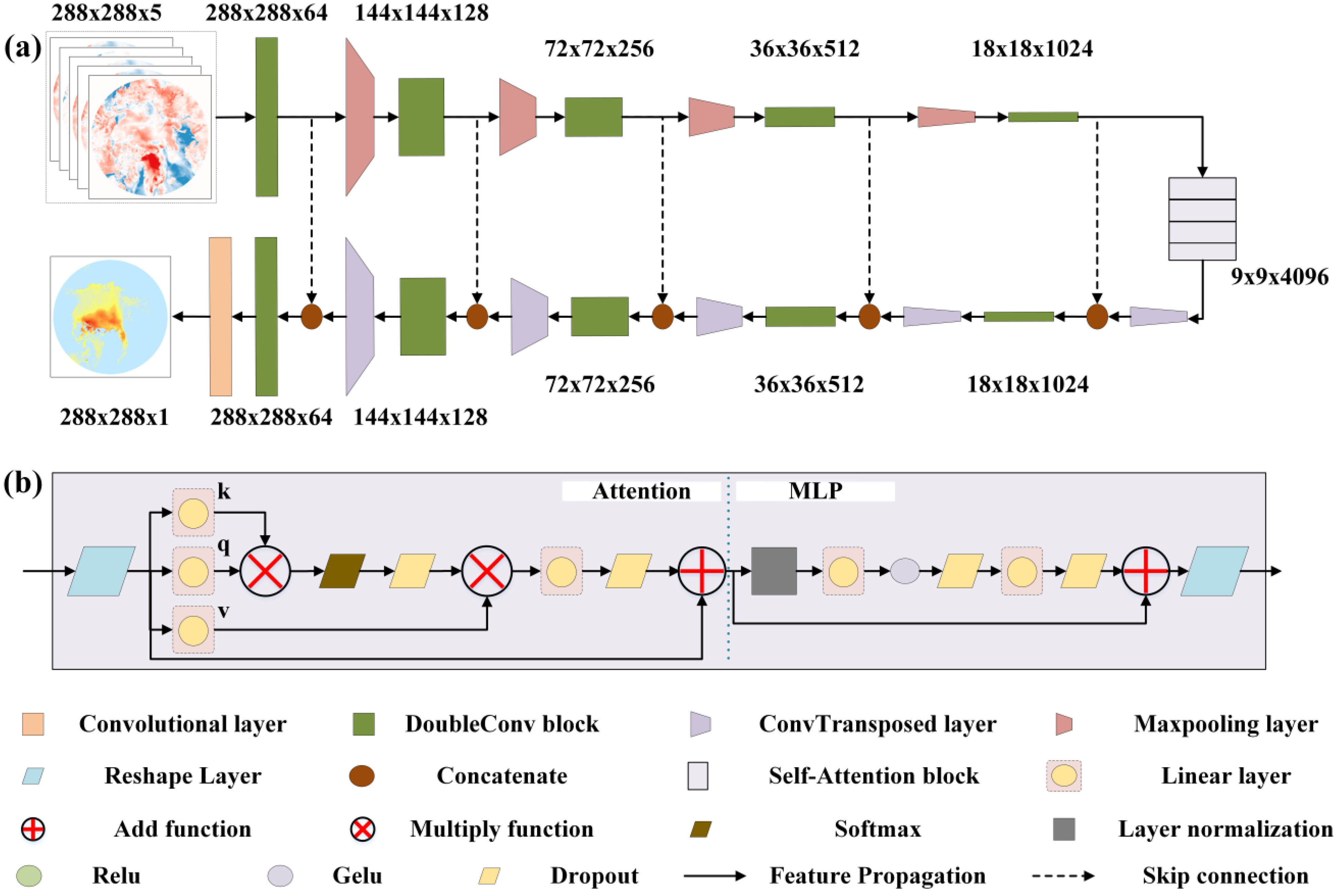
2.3. Self-Attention Convolutional Neural Network (SAC-Net)

Considering the spatiality and continuity of Arctic SIT, a novel deep learning-based self-attention convolutional neural network (SAC-Net) was designed for Arctic SIT estimation by combining a fully convolutional neural network [51] and a self-attention block [52] (Figure 3a).

2.3.1. Fully Convolutional Neural Network

The fully convolutional network was used as a baseline model for thermodynamic matrix spatial feature detection. It mainly consists of a downsampling branch and an up-sampling branch. The downsampling branch received a thermodynamic matrix with dimensions of 288 × 288 × 5, and it sampled them into highly abstract feature maps with dimensions of 18 × 18 × 1024 using continuous five double convolutional blocks and four max pooling layers. The upsampling branch was responsible for recovering the highly abstract feature map into a SIT prediction distribution with dimensions 288 × 288 × 1 by continuous five transposed convolutional layers, five double convolutional blocks, and a single convolutional layer. Additionally, skip connections were used to concatenate features with the same dimensions during upsampling and downsampling to compensate for the feature loss due to scale transformation.
Each double convolutional block consisted of two combined layers of a two-dimensional convolutional layer with a kernel size of 3 × 3 and a ReLU (rectified linear unit) activation layer for improving sensitivity to features. Each max pooling layer had a kernel size of 2 for feature dimension scaling. Each transposed convolutional layer had a kernel size of 2 × 2, a stride of 2, and served both feature abstraction and dimensional scaling. The single convolutional layer with a kernel size of 1 × 1 was used to organize the depth of the features to 1 to fit the thickness matrix of the sea ice.

2.3.2. Self-Attention Block

The feature maps exported from the downsampling branch were delivered into the self-attention block; feature maps of size 9 × 9 × 4096 exported from the self-attention block were then delivered to the upsampling branch.
The self-attention block contained four self-attention layers, and the structure of each self-attention layer, are shown in Figure 3b. Each self-attention layer comprised two components: attention and multilayer perceptron (MLP). In attention, the received feature maps were first reshaped to dimensions of 81 × 4096 to prepare for the subsequent operations, and three feature tensors (k, q, and v) were then obtained after applying three independent linear layers. The product of k and q was multiplied by v after SoftMax and dropout operations, and then fed into a linear layer and added with the reshaped features to obtain the output of attention. Subsequently, the features were fed into the MLP, where they first passed through a layer normalization, then through a linear layer with GeLU (Gaussian error linear units) and dropout functions, and finally through a linear layer with only the dropout function; they were then summed with the input features of the MLP. Finally, the output features were reshaped to their original dimensions of 9 × 9 × 4096.

2.4. Network Parameter Settings and Quantitative Evaluation Indices

During the training, the stochastic gradient descent (SGD) algorithm [53], which is one of the most commonly used algorithms, was used as the optimizer to minimize the loss and update the network parameters; the learning rate was set to 0.001. The batch size, number of training epochs, and the number of iterations in each epoch were set as 4, 100, and 1000, respectively.
To quantitatively evaluate the accuracy of the proposed method for SIT estimation, the BIAS, mean absolute error (MAE), root mean square error (RMSE), and Pearson correlation coefficient (r) were used. The formulae are as follows:
BIAS = 1 n i = 1 n ( y i x i )
MAE = 1 n i = 1 n | y i x i |
RMSE = 1 n i = 1 n ( y i x i ) 2
r = i = 1 n ( x i x ¯ ) ( y i y ¯ ) i = 1 n ( x i x ¯ ) 2 i = 1 n ( y i y ¯ ) 2
where n denotes the number of samples, and y i and x i denote prediction and truth value, respectively. x ¯ and y ¯ denote the average values of sample x and sample y, respectively.

3. Results

3.1. Model Performance on the Test Data

First, a Pearson correlation test was conducted between the SAC-Net-derived daily SIT values and the corresponding SIT values derived from the test CS2SMOS data from 2020 to 2021. Here, 50 values were randomly selected from each daily SIT map, and a total of 15,152 pairs of values participated in the statistics. The statistical results are shown in Figure 4a. Obviously, most sample points are concentrated near the 1:1 line, which shows that there is a remarkable correlation between CS2SMOS SIT and SAC-Net SIT with a Pearson correlation coefficient of 0.88. However, there is an overestimation in the interval of 2–3 m thickness. In statistical terms, 26 cm of MAE, 37 cm of RMSE, and 2 cm of bias for the test data are achieved. A p-value of approximately 0 indicates that statistics are significant. In general, the results of this model are in good agreement with those of CS2SMOS.
The SAC-Net proposed in this study was constructed by introducing a self-attention block using a fully convolutional network as the baseline model, and an ablation experiment was conducted to validate the performance improvement of the SAC-Net. In this experiment, an inter-comparison among SIT from the SAC-Net with four, three, two, and one attention layers, and the baseline network, was conducted. In addition, SIT from the FCN-8s [54], which is one of the popular networks for image processing, also participated in the comparison. The training and test data remained unchanged. When reducing the number of attention layers from four to one one by one (Figure 4a–d), there is a tendency for the evaluation index to become worse, indicating the effectiveness of four attention layers. When only the baseline network is available (Figure 4e), the r, RMSE, MAE, and bias values are 0.85, 42 cm, 30 cm, and 0.6 cm, respectively, which are worse than the results after the introduction of the attention layer, indicating the usefulness of the attention layer. Figure 4f shows that the results for FCN-8s are relatively much worse, indicating the proposed SAC-Net is a significant improvement over the FCN-8s.

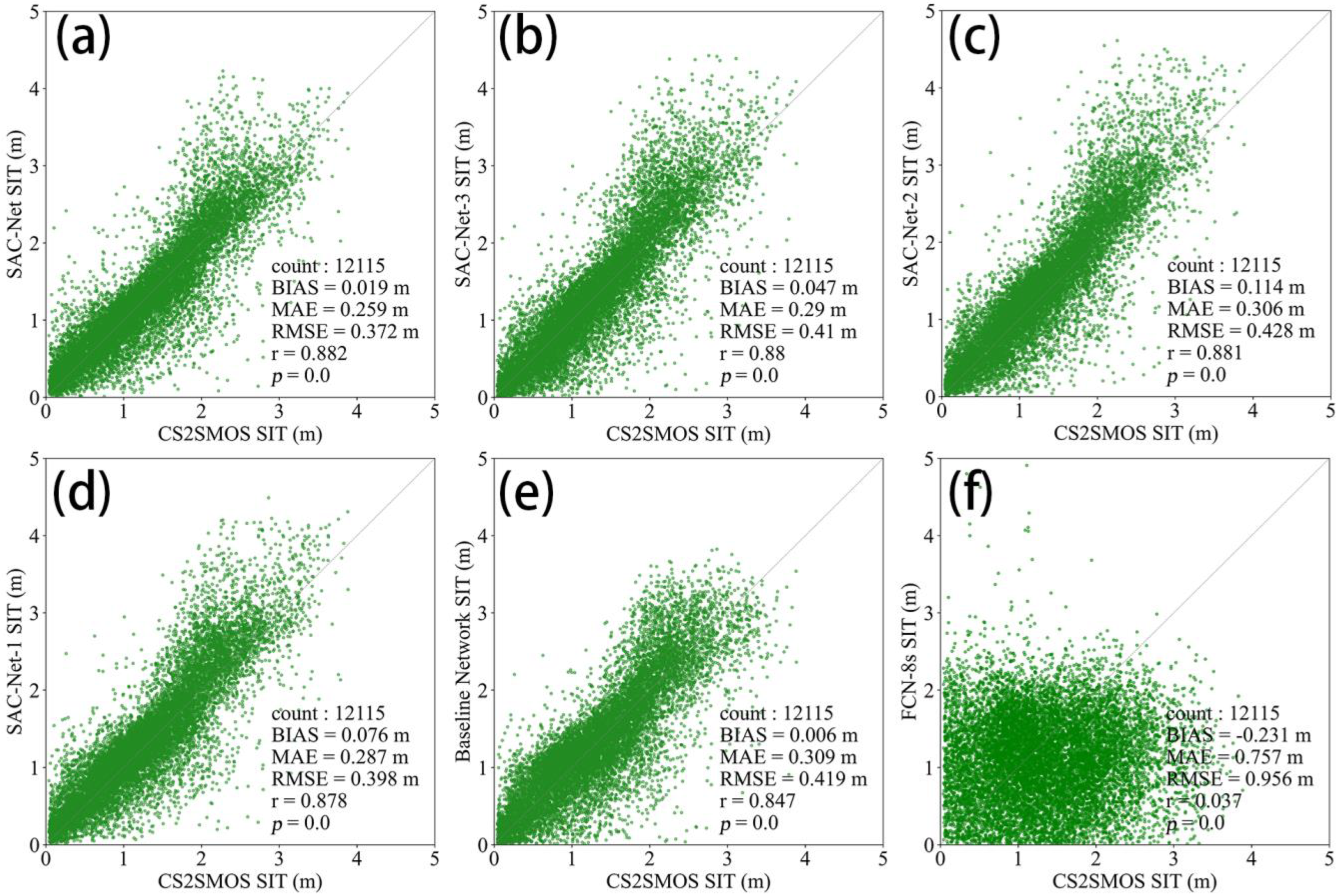
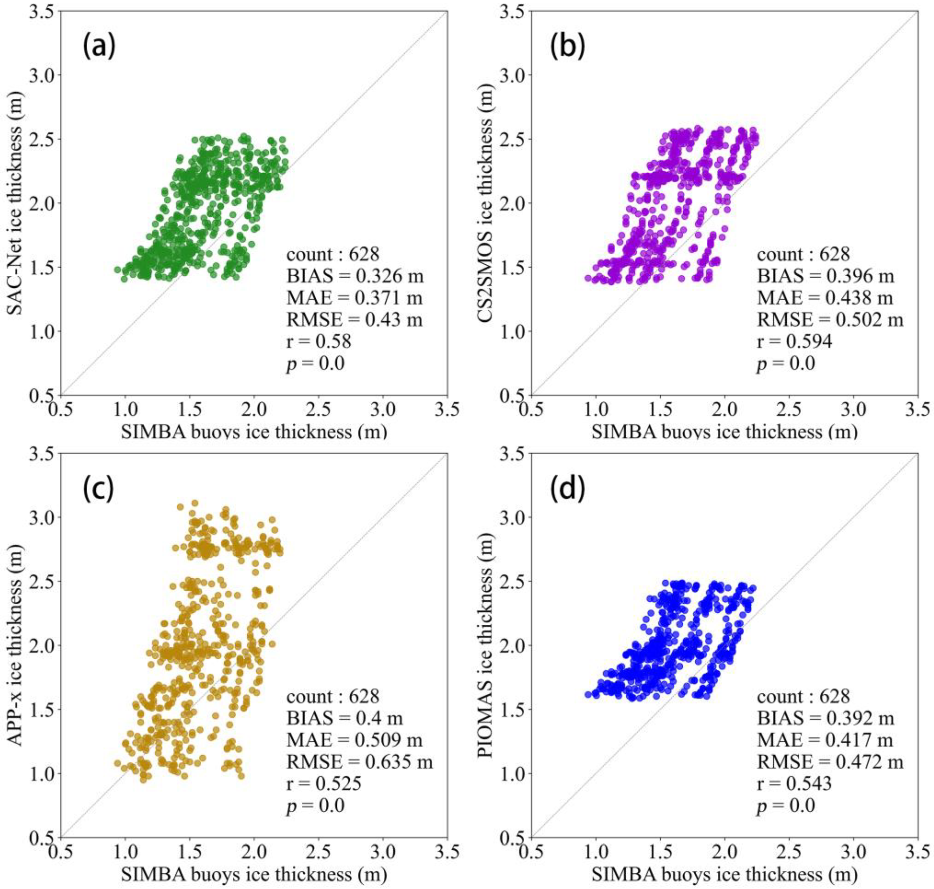
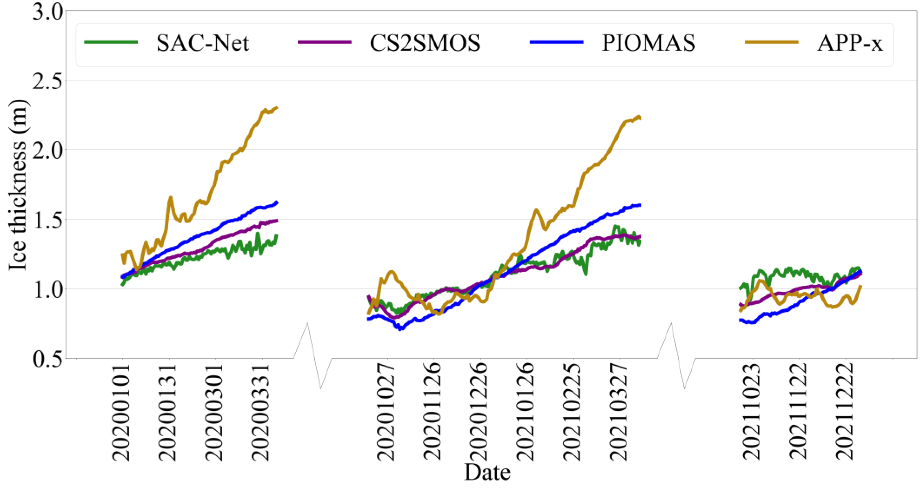
3.2. Accuracy Assessment of SIT with Other Methods Based on SIMBA Buoys

The accuracy of the CS2SMOS estimated, APP-x estimated, PIOMAS estimated, and the proposed thermodynamically estimated SIT was quantitatively assessed by a Pearson correlation analysis using the SIT measured by SIMBA buoys. In this experiment, SIT values were selected from CS2SMOS, APP-x, and SAC-Net based on the coordinates of SIMBA measurement points to form 628 pairs for statistical analyses. The results are shown in Figure 5.
Overall, the SIT from SIMBA is positively correlated with those from CS2SMOS, APP-x, and SAC-Net. Specifically, the r, RMSE, MAE, and bias of SIT between SIMBA and CS2SMOS are 0.59, 0.50 m, 0.44 m, and 0.40 m, respectively (Figure 5b). The quantitative evaluation data of APP-x and SIT measured from buoys are slightly worse than those of CS2SMOS and SIT measured from buoys, with an r of 0.53, RMSE of 0.64 m, MAE of 0.51 m, and bias of 0.4 m (Figure 5c). The data in Figure 5d reveals that SIMBA and PIOMAS have an r of 0.54, RMSE of 0.47, MAE of 0.42 m, and bias of 0.39. Figure 5a is the correlation statistics of SAC-Net and SIMBA, showing that the accuracy of the two is relatively good among the four products, as evidenced by the RMSE, MAE, and bias of 0.43 m, 0.37 m, and 0.33 m, respectively, although r is 0.58, slightly less than that of CS2SMOS.

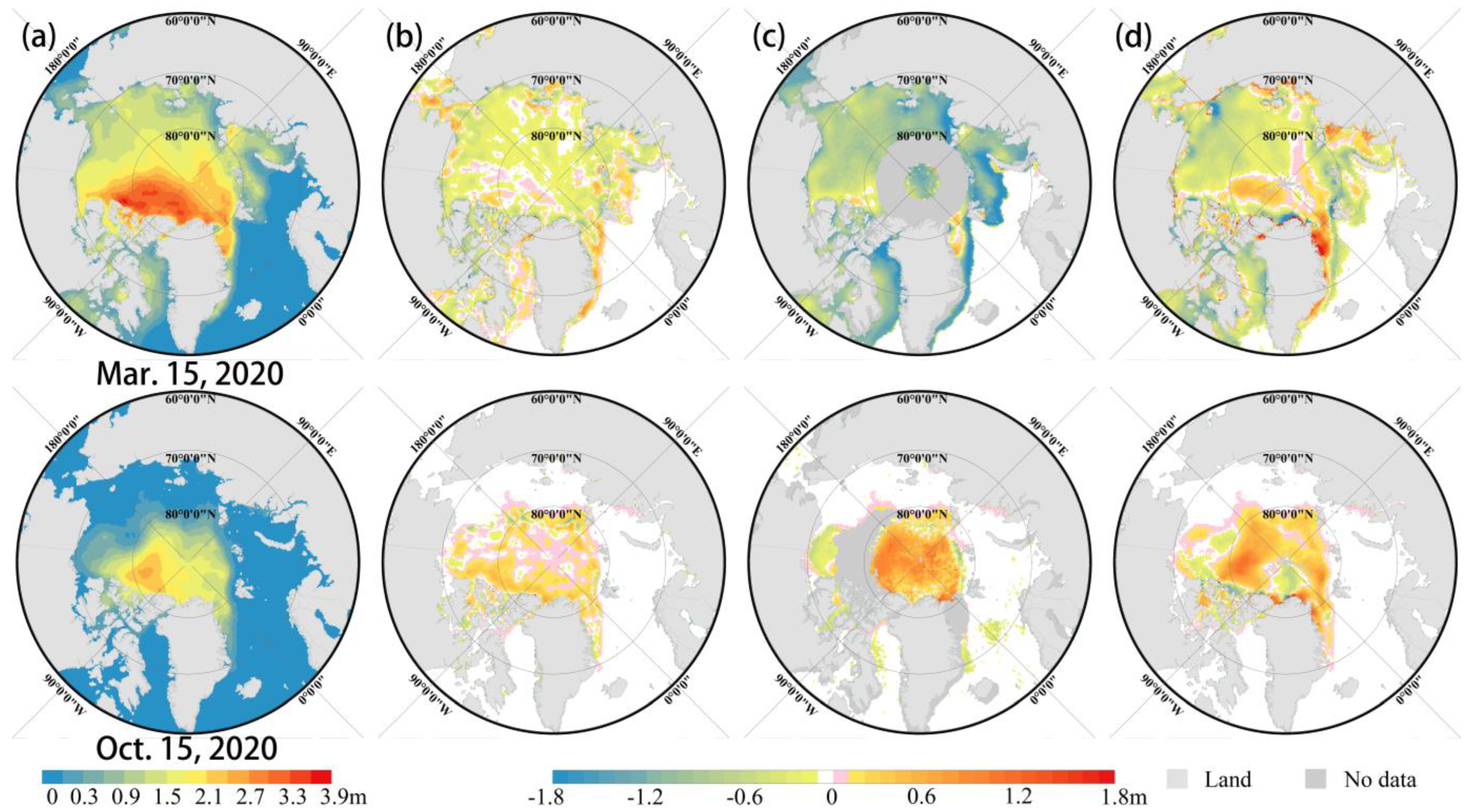
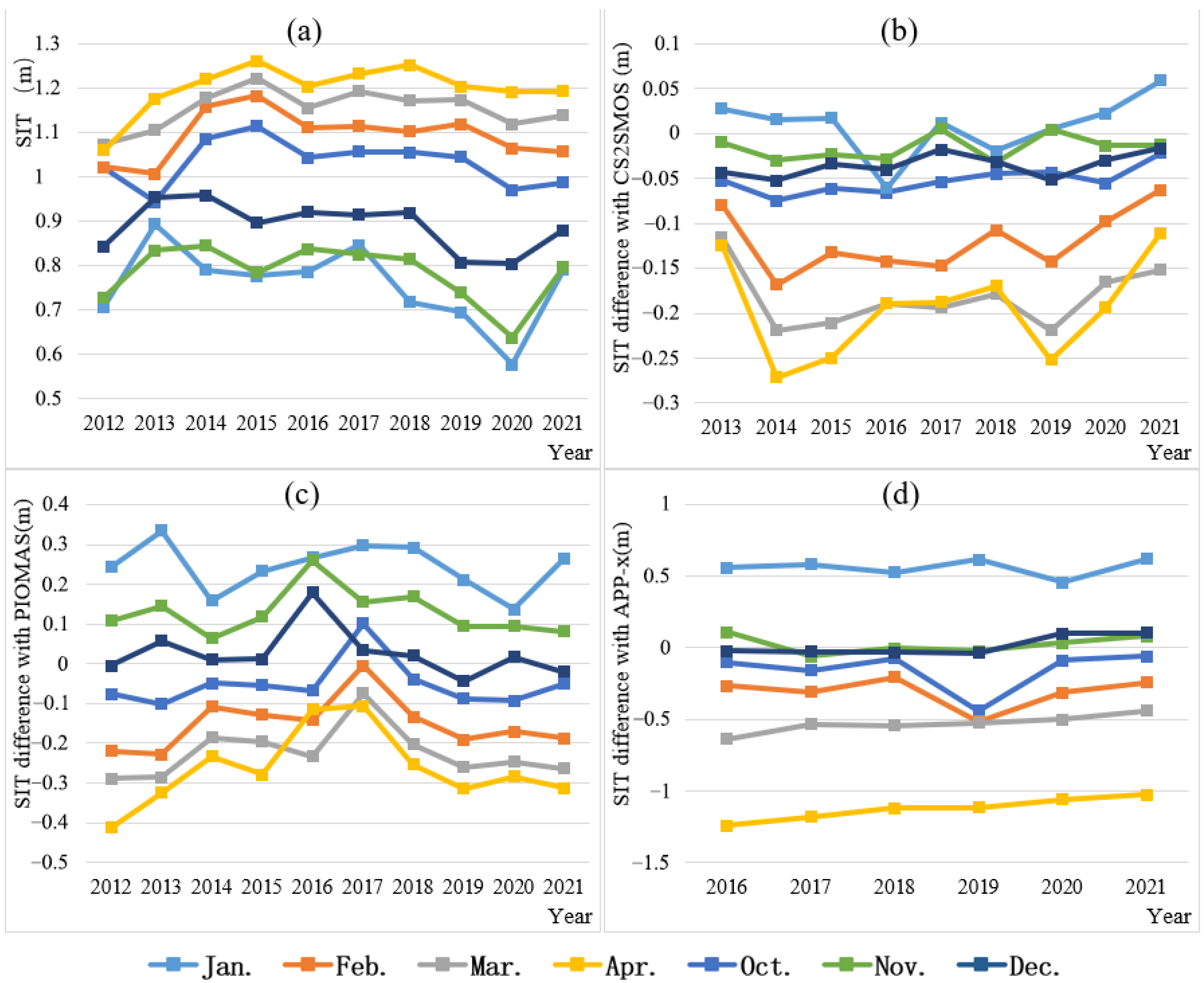
3.3. Comparisons among Different SIT Products

The average daily CS2SMOS-, APP-x-, PIOMAS-, and the SAC-Net thermodynamically estimated SITs from 2020 to 2021 were calculated and compared, as shown in Figure 6. Overall, the daily average SIT trend of each data set rises in winter. These four datasets have similar daily average SIT values from October to December every year. The daily average SIT of CS2SMOS (purple line) reaches its lowest value in October–November each year and then continues to increase in April of the following year. The daily average SIT of PIOMAS (blue line) is lower than that of CS2SMOS in the low-SIT period and higher in the high-SIT period. The daily average SIT of APP-x (brown line) is significantly higher, and the high value is at least 0.6 m higher than others. The green line, which indicates the daily average SIT derived from the proposed SAC-Net, matches well with the purple line, especially from October to December 2020, suggesting that our model data fits well with the CS2SMOS data. However, the SAC-Net results show that the value in March 2020 is slightly lower than the other three, slightly higher in October 2021, and the value fluctuates slightly.
The spatial distribution of SIT was derived from five selected parameters from the gridded ERA5 reanalysis data using SAC-Net. See Figure 7 for the SAC-Net derived SIT distribution on March 15th and 15 October 2020 and the differences with the other three products. As the target value of open water in the training dataset was set to −0.1 to avoid the influence of small data fluctuations, any value less than 0 in the obtained results was designated as 0. All distributions were cropped to a size of 282 × 282, projected onto the WGS 1984/NSIDC Sea Ice Polar Stereographic North grid with a spatial resolution of 25 km, and land-masked. Figure 7a shows that the sea ice edge is well defined by the SAC-Net SIT because of the substantial difference in thermodynamic parameters between the ice and water. On March 15th, the sea ice with a thickness of more than 2 m mainly appears in northern Greenland and the northern Canadian Archipelago, while the other areas are mainly the new ice, young ice, and the first-year ice during the Arctic freezing period, with obvious gradient change law. On October 15th, after summer melting, the original thick sea ice becomes thinner as a whole, and the original thin sea ice completely melts and disappears. The difference maps with the results of CS2SMOS show there is little difference between them, and the SIT from SAC-Net is slightly higher on 15th October (Figure 7b). Compared with APP-x, our results are lower in March and higher in October (Figure 7c). As shown in Figure 7d, in March, it is overestimated compared with PIOMAS on the east coast of Greenland, underestimated in the East Siberian Sea and the Beaufort Sea, and our results are high in October. Generally speaking, the spatial distribution of our SIT results is more in line with CS2SMOS.
Furthermore, we conducted an analysis of the interannual SIT variations over the past 10 years. In this experiment, monthly average SIT from the winter months of 2012 to 2021, as calculated by SAC-Net, were plotted as a line graph in Figure 8a. In addition, the differences between SAC-Net and CS2SMOS, PIOMAS, and APP-x were also calculated and plotted as graphs in Figure 8b–d. Due to missing data, the difference with CS2SMOS was only provided for the years 2013 to 2021, and the difference with APP-x was only provided for the years 2016 to 2021. From Figure 8a, it can be observed that the SIT reaches its maximum thickness of around 1.2 m in April almost every year between 2012 and 2021, and it reaches its minimum thickness of around 0.7 m in January every year. In 2020, the ice thickness in January reached the lowest value in ten years, at 0.58 m. Figure 8b shows that the differences in SIT between SAC-Net and CS2SMOS are within the range of [−0.3, 0.05] m, with the two being closest in SIT from October to January each year, and the differences increasing in February, March, and April. Figure 8c shows that SAC-Net and PIOMAS are closest in SIT from October to December each year, with overall differences within the range of [−0.4, 0.4] m. Figure 8d shows that the differences between SAC-Net and APP-x are relatively large, with differences within the range of [−1.3, 0.6] m, and the two are closest in ice thickness from October to December each year. In April, the absolute difference between the two exceeds 1 m. Overall, SAC-Net’s results are closest to those of CS2SMOS, with a higher reliability for SIT between October and December each year.

4. Discussion

In this study, we proposed a novel SAC-Net based on a neural network to build a model to simulate the potential influence relationship between thermodynamic parameters and SIT, and then attempted to automatically obtain the daily Arctic winter SIT. In SAC-Net, a self-attention block was introduced into a fully convolutional network to improve its performance. The self-attention block was developed and released by Google [52]; it has been updated and upgraded several times [55] and has often been used as an effective mechanism for improving neural network models for image feature extraction [56,57]. Preliminary experimental results demonstrated that the proposed method had a better consistency with CS2SMOS than was found before improvement, and that it correlated well with the SIT of SIMBA buoys and provided reliable estimates of SIT.
The previous results showed large differences between the SIT of SAC-Net and APP-x; therefore, we further investigated the potential reasons for this by comparing the pan-Arctic SIT distributions on 9 April 2020, when a relatively large daily SIT difference was observed between SAC-Net and APP-x (approximately −1 m). The SIT of PIOMAS and CS2SMOS were also compared. The result is shown in Figure 9. Notably, the overall SIT of APP-x (Figure 9c) is greater than 2 m, and thicker than that of any other satellite product, as evidenced by the studies conducted by [19,58]. There is a clear demarcation in the SIT obtained by SAC-Net, CS2SMOS, and PIOMAS, unlike that by APP-x. In particular, the SIT in the marginal ice zone was compared in each of the four products. The first row in Figure 9 is located in Nansen Basin in the Arctic, and the second row is located in the Chukchi Sea in the Arctic. It shows that the SIT of different products in the same position is quite different. At both sites, APP-x has a SIT of about 2 m, while the other three have SITs below 1 m. The SIT variation of SAC-Net, CS2SMOS, and PIOMAS is more reasonable than the cliff-like SIT of APP-x in the marginal ice zone, and the spatial gradient variation of SAC-Net and CS2SMOS is very similar. It has been revealed that the SIT of APP-x shows little interannual variation and SIT gradient variation [58]. This explains why the bias of SIT between SAC-Net and APP-x in Figure 5, Figure 6 and Figure 7 is prominent, indicating that the sea ice distribution of SAC-Net is more reliable.
The error sources of this study mainly come from two aspects. The first is the inherent error of the target data CS2SMOS in the training dataset. When deriving the SIT from the freeboard measured by CryoSat-2, uncertainties in the snow depth, snow, ice, and water density can affect the final SIT results [59]. Additionally, errors arising when filling the CryoSat-2 data gaps or during fusion with the SMOS data can lead to increased uncertainty in the results [43]. As a matter of course, these errors are also considered by SAC-Net. The second error source is the quality of the thermodynamic data. Inaccurate input data lead to inaccurate SIT. Furthermore, there may be other factors affecting SIT that are not included in the selected five thermodynamic data, and the model may not be able to capture the full complexity of the relationships between thermodynamic variables and SIT.

5. Conclusions

In this study, a neural network named SAC-Net was proposed to build a model to simulate the potential influencing relationship between thermodynamic parameters and SIT more parsimoniously, and to attempt to automatically obtain the daily Arctic SIT. SAC-Net used a fully convolutional network as the baseline model to detect spatial features from thermodynamic data, and also introduced a self-attention block to further explore the deeper hidden connections of abstract features and to achieve a better feature fit. To construct a suitable training dataset, the five thermodynamic parameters (SSHF, SLHF, T2M, SKT, and TSN) from ERA5 and the SIT from CS2SMOS were used as input and target, where the five selected thermodynamic parameters are the most relevant to SIT variation among the available parameters of ERA5, and the SIT data of CS2SMOS have proven to be highly reliable and widely used in polar sea ice studies. The SAC-Net was trained on the training dataset to obtain a neural network model for estimating SIT from Arctic thermodynamic parameters.
The experimental results of the model performance test showed that the SIT obtained from untrained thermodynamic data in 2020–2021 can achieve high consistency with CS2SMOS, and the ablation experiments suggested the effectiveness of the improved components of the SAC-Net. When verifying the accuracy of CS2SMOS-, APP-x-, PIOMAS-, and SAC-Net thermodynamically estimated SIT using SIT measurements from SIMBA buoys, the r value between SIT from SAC-Net and SIMBA reached 0.58 and the RMSE was 0.43 m, which was better than those of APP-x and PIOMAS. In terms of the time series of SIT changes, from 2020 to 2021, the daily average SIT trend of SAC-Net and CS2SMOS was very similar, and the bias between them was very small; however, the maximum bias between SAC-Net and PIOMAS was about 0.4 m, and the maximum bias between SAC-Net and APP-x was over 1 m. In terms of the spatial distribution of SIT, the difference in SIT distribution showed a large difference between SAC-Net and APP-x, as the SIT of APP-x is unreasonably large, while the difference with CS2SMOS is minimal. The comparisons of interannual SIT variations over the past 10 years among SIT products revealed that the SAC-Net has higher SIT reliability between October and December each year.
SAC-Net proved the feasibility and effectiveness of modeling using thermodynamic data and SIT by the neural network, and successfully obtains reliable daily SIT data for the Arctic winter. This method could complement existing thermodynamic-based SIT products to assist with research on Arctic sea ice and global climate change. Future research could consider using more comprehensive and precise environmental data related to sea ice changes, as well as SIT data (such as buoys) to construct models. This may result in more reliable SIT estimation models. Additionally, it is worthwhile to investigate how to obtain SIT in summer and the driving forces behind sea ice changes.

Author Contributions

Conceptualization, X.P. and Q.J.; methodology, Z.L. and X.Y.; software, Z.L.; validation, Z.L., P.F., Y.C. (Yizhuo Chen) and Z.Y.; formal analysis, Z.L. and P.F.; investigation, Z.L.; resources, Z.L., P.F. and Y.C. (Ying Chen); data curation, Z.L. and P.F.; writing—original draft preparation, Z.L.; writing—review and editing, X.P., Q.J., Z.L., P.F., X.Y., Y.C. (Yizhuo Chen), Y.C. (Ying Chen) and Z.Y.; visualization, Z.L. and Y.C. (Ying Chen); supervision, X.P. and Q.J.; project administration, X.P. and Q.J.; funding acquisition, X.P. and Q.J. All authors have read and agreed to the published version of the manuscript.

Funding

This work was partly supported by the National Natural Science Foundation of China (Grant NO. 42076235) and the Fundamental Research Funds for the Central Universities (Grant NO. 2042022kf0018).

Data Availability Statement

Not applicable.

Conflicts of Interest

The authors declare no conflict of interest.

References

  1. Kwok, R. Deformation of the Arctic Ocean Sea Ice Cover between November 1996 and April 1997: A Qualitative Survey. In Proceedings of the IUTAM Symposium on Scaling Laws in Ice Mechanics and Ice Dynamics, Fairbanks, AK, USA, 13–16 June 2001; pp. 315–322. [Google Scholar] [CrossRef]
  2. Perovich, D.K.; Nghiem, S.V.; Markus, T.; Schweiger, A. Seasonal Evolution and Interannual Variability of the Local Solar Energy Absorbed by the Arctic Sea Ice-Ocean System. J. Geophys. Res. Ocean. 2007, 112, 1–13. [Google Scholar] [CrossRef]
  3. Lee, S.M.; Meier, W.N.; Sohn, B.J.; Shi, H.; Gasiewski, A.J. Estimation of Arctic Basin-Scale Sea Ice Thickness from Satellite Passive Microwave Measurements. IEEE Trans. Geosci. Remote Sens. 2021, 59, 5841–5850. [Google Scholar] [CrossRef]
  4. Demir, O.; Jezek, K.; Brogioni, M.; Macelloni, G.; Kaleschke, L.; Johnson, J. Studies of the Retrieval of Sea Ice Thickness and Salinity with Wideband Microwave Radiometry. In Proceedings of the 2021 IEEE International Geoscience and Remote Sensing Symposium IGARSS, Brussels, Belgium, 11–16 July 2021; pp. 5544–5545. [Google Scholar] [CrossRef]
  5. Meredith, M.; Sommerkorn, M.; Cassotta, S.; Derksen, C.; Ekaykin, A.; Hollowed, A.; Kofinas, G.; Mackintosh, A.; Melbourne-Thomas, J.; Muelbert, M.M.C.; et al. Polar Regions. In IPCC Special Report on the Ocean and Cryosphere in a Changing Climate; Pörtner, H.-O., Roberts, D.C., Masson-Delmotte, V., Zhai, P., Tignor, M., Poloczanska, E., Mintenbeck, K., Alegría, A., Nicolai, M., Okem, A., et al., Eds.; Cambridge University Press: Cambridge, UK; New York, NY, USA, 2019; pp. 203–320. ISBN 9781009157964. [Google Scholar]
  6. Richter-Menge, J.A.; Perovich, D.K.; Elder, B.C.; Claffey, K.; Rigor, I.; Ortmeyer, M. Ice Mass-Balance Buoys: A Tool for Measuring and Attributing Changes in the Thickness of the Arctic Sea-Ice Cover. Ann. Glaciol. 2006, 44, 205–210. [Google Scholar] [CrossRef] [Green Version]
  7. Fukamachi, Y.; Simizu, D.; Ohshima, K.I.; Eicken, H.; Mahoney, A.R.; Iwamoto, K.; Moriya, E.; Nihashi, S. Sea-Ice Thickness in the Coastal Northeastern Chukchi Sea from Moored Ice-Profiling Sonar. J. Glaciol. 2017, 63, 888–898. [Google Scholar] [CrossRef] [Green Version]
  8. Matsumoto, M.; Yoshimura, M.; Naoki, K.; Cho, K.; Wakabayashi, H. Ground Penetrating Radar Data Interpretation Using Electromagnetic Field Analysis for Sea Ice Thickness Measurement. Int. Arch. Photogramm. Remote Sens. Spat. Inf. Sci. 2019, 42, 47–50. [Google Scholar] [CrossRef] [Green Version]
  9. Stroeve, J.; Barrett, A.; Serreze, M.; Schweiger, A. Erratum: Using Records from Submarine, Aircraft and Satellites to Evaluate Climate Model Simulations of Arctic Sea Ice Thickness (Cryosphere (2014) 8 (1839–1854)). Cryosphere 2015, 9, 81. [Google Scholar] [CrossRef] [Green Version]
  10. Kwok, R. Satellite Remote Sensing of Sea-Ice Thickness and Kinematics: A Review. J. Glaciol. 2011, 56, 1129–1140. [Google Scholar] [CrossRef] [Green Version]
  11. Kwok, R.; Kacimi, S.; Webster, M.A.; Kurtz, N.T.; Petty, A.A. Arctic Snow Depth and Sea Ice Thickness from ICESat-2 and CryoSat-2 Freeboards: A First Examination. J. Geophys. Res. Ocean. 2020, 125, 1–19. [Google Scholar] [CrossRef]
  12. Xu, Y.; Li, H.; Liu, B.; Xie, H.; Ozsoy-Cicek, B. Deriving Antarctic Sea-Ice Thickness from Satellite Altimetry and Estimating Consistency for NASA’s ICESat/ICESat-2 Missions. Geophys. Res. Lett. 2021, 48, 1–12. [Google Scholar] [CrossRef]
  13. Pang, X.; Chen, Y.; Ji, Q.; Li, G.; Shi, L.; Lan, M.; Liang, Z. An Improved Algorithm for the Retrieval of the Antarctic Sea Ice Freeboard and Thickness from ICESat-2 Altimeter Data. Remote Sens. 2022, 14, 1069. [Google Scholar] [CrossRef]
  14. Xiao, F.; Zhang, S.; Li, J.; Geng, T.; Xuan, Y.; Li, F. Arctic Sea Ice Thickness Variations from CryoSat-2 Satellite Altimetry Data. Sci. China Earth Sci. 2021, 64, 1080–1089. [Google Scholar] [CrossRef]
  15. Ji, Q.; Li, B.; Pang, X.; Zhao, X.; Lei, R. Arctic Sea Ice Density Observation and Its Impact on Sea Ice Thickness Retrieval from CryoSat–2. Cold Reg. Sci. Technol. 2021, 181, 103177. [Google Scholar] [CrossRef]
  16. Petty, A.A.; Kurtz, N.T.; Kwok, R.; Markus, T.; Neumann, T.A. Winter Arctic Sea Ice Thickness from ICESat-2 Freeboards. J. Geophys. Res. Ocean. 2020, 125, 1–28. [Google Scholar] [CrossRef]
  17. Warren, S.G.; Rigor, I.G.; Untersteiner, N.; Radionov, V.F.; Bryazgin, N.N.; Aleksandrov, Y.I.; Colony, R. Snow Depth on Arctic Sea Ice. J. Clim. 1999, 12, 1814–1829. [Google Scholar] [CrossRef]
  18. Laxon, S.; Peacock, H.; Smith, D. High Interannual Variability of Sea Ice Thickness in the Arctic Region. Nature 2003, 425, 947–950. [Google Scholar] [CrossRef]
  19. Wang, X.; Key, J.; Kwok, R.; Zhang, J. Comparison of Arctic Sea Ice Thickness from Satellites, Aircraft, and PIOMAS Data. Remote Sens. 2016, 8, 713. [Google Scholar] [CrossRef] [Green Version]
  20. Yu, Y.; Rothrock, D.A. Thin Ice Thickness from Satellite Thermal Imagery. J. Geophys. Res. C Ocean. 1996, 101, 25753–25766. [Google Scholar] [CrossRef]
  21. Kaleschke, L.; Maaß, N.; Haas, C.; Hendricks, S.; Heygster, G.; Tonboe, R.T. A Sea-Ice Thickness Retrieval Model for 1.4 GHz Radiometry and Application to Airborne Measurements over Low Salinity Sea-Ice. Cryosphere 2010, 4, 583–592. [Google Scholar] [CrossRef] [Green Version]
  22. Tian-Kunze, X.; Kaleschke, L.; Maaß, N.; Mäkynen, M.; Serra, N.; Drusch, M.; Krumpen, T. SMOS-Derived Thin Sea Ice Thickness: Algorithm Baseline, Product Specifications and Initial Verification. Cryosphere 2014, 8, 997–1018. [Google Scholar] [CrossRef] [Green Version]
  23. Gupta, M.; Gabarro, C.; Turiel, A.; Portabella, M.; Martinez, J. On the Retrieval of Sea-Ice Thickness Using SMOS Polarization Differences. J. Glaciol. 2019, 65, 481–493. [Google Scholar] [CrossRef] [Green Version]
  24. Huntemann, M.; Heygster, G.; Kaleschke, L.; Krumpen, T.; Mäkynen, M.; Drusch, M. Empirical Sea Ice Thickness Retrieval during the Freeze-up Period from SMOS High Incident Angle Observations. Cryosphere 2014, 8, 439–451. [Google Scholar] [CrossRef] [Green Version]
  25. Kaleschke, L.; Tian-Kunze, X.; Maaß, N.; Beitsch, A.; Wernecke, A.; Miernecki, M.; Müller, G.; Fock, B.H.; Gierisch, A.M.U.; Schlünzen, K.H.; et al. SMOS Sea Ice Product: Operational Application and Validation in the Barents Sea Marginal Ice Zone. Remote Sens. Environ. 2016, 180, 264–273. [Google Scholar] [CrossRef]
  26. Kaleschke, L.; Tian-Kunze, X.; Maas, N.; Ricker, R.; Hendricks, S.; Drusch, M. Improved Retrieval of Sea Ice Thickness from SMOS and CryoSat-2. In Proceedings of the 2015 IEEE International Geoscience and Remote Sensing Symposium (IGARSS), Milan, Italy, 26–31 July 2015; pp. 5232–5235. [Google Scholar] [CrossRef]
  27. Wang, X.; Key, J.R.; Liu, Y. A Thermodynamic Model for Estimating Sea and Lake Ice Thickness with Optical Satellite Data. J. Geophys. Res. Ocean. 2010, 115, 1–14. [Google Scholar] [CrossRef] [Green Version]
  28. Olonscheck, D.; Mauritsen, T.; Notz, D. Arctic Sea-Ice Variability Is Primarily Driven by Atmospheric Temperature Fluctuations. Nat. Geosci. 2019, 12, 430–434. [Google Scholar] [CrossRef]
  29. Notz, D.; Jahn, A.; Holland, M.; Hunke, E.; Massonnet, F.; Stroeve, J.; Tremblay, B.; Vancoppenolle, M. The CMIP6 Sea-Ice Model Intercomparison Project (SIMIP): Understanding Sea Ice through Climate-Model Simulations. Geosci. Model Dev. 2016, 9, 3427–3446. [Google Scholar] [CrossRef] [Green Version]
  30. Yang, C.Y.; Liu, J.; Xu, S. Seasonal Arctic Sea Ice Prediction Using a Newly Developed Fully Coupled Regional Model with the Assimilation of Satellite Sea Ice Observations. J. Adv. Model. Earth Syst. 2020, 12, 1–25. [Google Scholar] [CrossRef] [Green Version]
  31. Zhang, J.; Rothrock, D.A. Modeling Global Sea Ice with a Thickness and Enthalpy Distribution Model in Generalized Curvilinear Coordinates. Mon. Weather Rev. 2003, 131, 845–861. [Google Scholar] [CrossRef]
  32. Shi, Q.; Yang, Q.; Mu, L.; Wang, J.; Massonnet, F.; Mazloff, M.R. Evaluation of Sea-Ice Thickness from Four Reanalyses in the Antarctic Weddell Sea. Cryosphere 2021, 15, 31–47. [Google Scholar] [CrossRef]
  33. Zhu, X.X.; Tuia, D.; Mou, L.; Xia, G.S.; Zhang, L.; Xu, F.; Fraundorfer, F. Deep Learning in Remote Sensing: A Review. IEEE Geosci. Remote Sens. Mag. 2017, 5, 8–36. [Google Scholar] [CrossRef] [Green Version]
  34. Yu, Y.; Samali, B.; Rashidi, M.; Mohammadi, M.; Nguyen, T.N.; Zhang, G. Vision-Based Concrete Crack Detection Using a Hybrid Framework Considering Noise Effect. J. Build. Eng. 2022, 61, 105246. [Google Scholar] [CrossRef]
  35. Yu, Y.; Liang, S.; Samali, B.; Nguyen, T.N.; Zhai, C.; Li, J.; Xie, X. Torsional Capacity Evaluation of RC Beams Using an Improved Bird Swarm Algorithm Optimised 2D Convolutional Neural Network. Eng. Struct. 2022, 273, 115066. [Google Scholar] [CrossRef]
  36. Liang, Z.; Pang, X.; Ji, Q.; Zhao, X.; Li, G.; Chen, Y. An Entropy-Weighted Network for Polar Sea Ice Open Lead Detection from Sentinel-1 SAR Images. IEEE Trans. Geosci. Remote Sens. 2022, 60, 1–14. [Google Scholar] [CrossRef]
  37. Zakhvatkina, N.; Smirnov, V.; Bychkova, I. Satellite SAR Data-Based Sea Ice Classification: An Overview. Geosci. 2019, 9, 152. [Google Scholar] [CrossRef] [Green Version]
  38. Jun Kim, Y.; Kim, H.C.; Han, D.; Lee, S.; Im, J. Prediction of Monthly Arctic Sea Ice Concentrations Using Satellite and Reanalysis Data Based on Convolutional Neural Networks. Cryosphere 2020, 14, 1083–1104. [Google Scholar] [CrossRef] [Green Version]
  39. Chi, J.; Kim, H.C. Retrieval of Daily Sea Ice Thickness from AMSR2 Passive Microwave Data Using Ensemble Convolutional Neural Networks. GIScience Remote Sens. 2021, 58, 812–830. [Google Scholar] [CrossRef]
  40. Dawson, G.; Landy, J.; Tsamados, M.; Komarov, A.S.; Howell, S.; Heorton, H.; Krumpen, T. A 10-Year Record of Arctic Summer Sea Ice Freeboard from CryoSat-2. Remote Sens. Environ. 2022, 268, 112744. [Google Scholar] [CrossRef]
  41. Landy, J.C.; Dawson, G.J.; Tsamados, M.; Bushuk, M.; Stroeve, J.C.; Howell, S.E.L.; Krumpen, T.; Babb, D.G.; Komarov, A.S.; Heorton, H.D.B.S.; et al. A Year-Round Satellite Sea-Ice Thickness Record from CryoSat-2. Nature 2022, 609, 517–522. [Google Scholar] [CrossRef]
  42. Muñoz Sabater, J. ERA5-Land Hourly Data from 1981 to Present. Copernic. Clim. Chang. Serv. Clim. Data Store (CDS) 2019, 13, 4349–4383. [Google Scholar] [CrossRef]
  43. Ricker, R.; Hendricks, S.; Kaleschke, L.; Tian-Kunze, X.; King, J.; Haas, C. A Weekly Arctic Sea-Ice Thickness Data Record from Merged CryoSat-2 and SMOS Satellite Data. Cryosphere 2017, 11, 1607–1623. [Google Scholar] [CrossRef] [Green Version]
  44. Key, J.; Wang, X.; Liu, Y.; Dworak, R.; Letterly, A. The AVHRR Polar Pathfinder Climate Data Records. Remote Sens. 2016, 8, 167. [Google Scholar] [CrossRef] [Green Version]
  45. Zhang, J.; Rothrock, D. A Thickness and Enthalpy Distribution Sea-Ice Model. J. Phys. Oceanogr. 2001, 31, 2986–3001. [Google Scholar] [CrossRef]
  46. Thorndike, A.S.; Rothrock, D.A.; Maykut, G.A.; Colony, R. The Thickness Distribution of Sea Ice. J. Geophys. Res. 1975, 80, 4501–4513. [Google Scholar] [CrossRef]
  47. Ruibo, L.; Bin, C.; Mario, H.; Guangyu, Z. Snow Depth and Sea Ice Thickness Derived from the Measurements of SIMBA Buoys Deployed in the Arctic Ocean during the Legs 1a, 1, and 3 of the MOSAiC Campaign in 2019–2020. PANGAEA 2021. [Google Scholar] [CrossRef]
  48. Jackson, K.; Wilkinson, J.; Maksym, T.; Meldrum, D.; Beckers, J.; Haas, C.; Mackenzie, D. A Novel and Low-Cost Sea Ice Mass Balance Buoy. J. Atmos. Ocean. Technol. 2013, 30, 2676–2688. [Google Scholar] [CrossRef] [Green Version]
  49. Deser, C.; Walsh, J.E.; Timlin, M.S. Arctic Sea Ice Variability in the Context of Recent Atmospheric Circulation Trends. J. Clim. 2000, 13, 617–633. [Google Scholar] [CrossRef]
  50. Lepparanta, M. A Review of Analytical Models of Sea-ice Growth. Atmosphere-Ocean 1993, 31, 123–138. [Google Scholar] [CrossRef]
  51. Shelhamer, E.; Long, J.; Darrell, T. Fully Convolutional Networks for Semantic Segmentation. IEEE Trans. Pattern Anal. Mach. Intell. 2017, 39, 640–651. [Google Scholar] [CrossRef]
  52. Vaswani, A.; Shazeer, N.; Parmar, N.; Uszkoreit, J.; Jones, L.; Gomez, A.N.; Kaiser, Ł.; Polosukhin, I. Attention Is All You Need. IEEE Ind. Appl. Mag. 2017, 8, 8–15. [Google Scholar] [CrossRef] [Green Version]
  53. Ruder, S. An Overview of Gradient Descent Optimization Algorithms. arXiv 2016, arXiv:1609.04747, 1–14. [Google Scholar]
  54. Shelhamer, E.; Long, J.; Darrell, T. Fully Convolutional Networks for Semantic Segmentation. In Proceedings of the British Machine Vision Conferece, York, UK, 19–22 September 2016; pp. 124.1–124.14. [Google Scholar] [CrossRef]
  55. Cordonnier, J.-B.; Loukas, A.; Jaggi, M. On the Relationship between Self-Attention and Convolutional Layers. arXiv 2019, arXiv:1911.03584. [Google Scholar]
  56. Zhou, Y.; Wang, F.; Zhao, J.; Yao, R.; Chen, S.; Ma, H. Spatial-Temporal Based Multi-Head Self-Attention for Remote Sensing Image Change Detection. IEEE Trans. Circuits Syst. Video Technol. 2022, 32, 6615–6626. [Google Scholar] [CrossRef]
  57. Cao, R.; Fang, L.; Lu, T.; He, N. Self-Attention-Based Deep Feature Fusion for Remote Sensing Scene Classification. IEEE Geosci. Remote Sens. Lett. 2021, 18, 43–47. [Google Scholar] [CrossRef]
  58. Sallila, H.; Farrell, S.L.; McCurry, J.; Rinne, E. Assessment of Contemporary Satellite Sea Ice Thickness Products for Arctic Sea Ice. Cryosphere 2019, 13, 1187–1213. [Google Scholar] [CrossRef] [Green Version]
  59. Kurtz, N.T.; Galin, N.; Studinger, M. An Improved CryoSat-2 Sea Ice Freeboard Retrieval Algorithm through the Use of Waveform Fitting. Cryosphere 2014, 8, 1217–1237. [Google Scholar] [CrossRef] [Green Version]
Figure 1. Study area and dataset. (a) An example of the Arctic 2 m temperature data distribution for 1 January 2021, obtained from the ERA5 reanalysis data; (b) an example of the Arctic SIT distribution on 1 January 2021, obtained from CS2SMOS. Grey regions represent the land. Green points represent the SIMBA buoys.
Remotesensing 15 01887 g001
Figure 2. Correlation coefficient statistics between each candidate thermodynamic parameter and Arctic winter SIT.
Remotesensing 15 01887 g002
Figure 3. Structure of SAC-Net as proposed in this study. (a) The overall structure of the proposed SAC-Net and the 3D numbers representing the feature dimensions after the convolutional operation; (b) the structure of the self-attention block.
Remotesensing 15 01887 g003
Figure 4. Statistical accuracies of the proposed SIT estimation model using the test data. (ad) Scatter plots of the SIT estimated by the SAC-Net with four, three, two, and one attention layers vs. CS2SMOS SIT; (e) scatter plot of baseline network estimated SIT vs. CS2SMOS SIT; (f) scatter plot of FCN-8s estimated SIT vs. CS2SMOS SIT.
Remotesensing 15 01887 g004
Figure 5. Statistical accuracy comparisons using 628 matched samples from SIMBA buoys, the proposed SAC-Net, CS2SMOS, APP-x, and PIOMAS SIT. (a) Scatter plot of SIMBA buoys SIT vs. SAC-Net SIT; (b) scatter plot of SIMBA buoys SIT vs. CS2SMOS SIT; (c) scatter plot of SIMBA buoys SIT vs. APP-x SIT; (d) scatter plot of SIMBA buoys SIT vs. PIOMAS SIT.
Remotesensing 15 01887 g005
Figure 6. Comparison of daily average SIT from different SIT products in winter during 2020–2021. The lines in green, purple, blue, and brown denote the trend of SIT from SAC-Net thermodynamically estimated, CS2SMOS estimated, PIOMAS estimated, and APP-x estimated SIT with time.
Remotesensing 15 01887 g006
Figure 7. Daily spatial distribution of SIT from SAC-Net and difference with other SIT products. (a) SAC-Net thermodynamically estimated SIT maps on March 15th and 15 October 2020, with a separate color bar; (b) difference with CS2SMOS estimated SIT maps; (c) difference with APP-x estimated SIT maps; (d) difference with PIOMAS estimated SIT maps. The plots in columns (bd) have a common color bar.
Remotesensing 15 01887 g007
Figure 8. Interannual variations in Arctic sea ice thickness between 2012 and 2021, along with a comparison to various products. (a) The interannual variation of monthly mean SIT obtained by SAC-Net; (bd) depict the differences between monthly average SIT obtained by SAC-Net and those obtained by CS2SMOS, PIOMAS, and APP-x, respectively.
Remotesensing 15 01887 g008
Figure 9. Comparison of the details of SIT distribution using different methods on 9 April 2020. Each column represents the SIT distribution of different methods. (a) SAC-Net thermodynamically estimated; (b) CS2SMOS estimated; (c) APP-x estimated; (d) PIOMAS estimated. Each row represents a comparison of different regions: NANSEN BASIN (first row) and CHUKCHI SEA (second row).
Remotesensing 15 01887 g009
Table 1. Information on data used in this study.
DatasetGrid ResolutionTemporal RangeGapTheoretical BasisUsed for
ERA50.25°2012–2019/4D-Var data assimilation and CY41R2 model [42]Training
2020–2021Testing
CS2SMOS25 km2012–201910 April–14 OctoberThermodynamic and hydrostatic-equilibrium [43]Training
2020–2021Testing
APP-x25 km2020/Thermodynamic [27,44]Comparison
PIOMAS/2020/Thermodynamic [31,45,46]Comparison
SIMBA/2020/Thermistor string [47,48].Comparison
Table 2. List of candidate parameters.
Parameter NameAbbrUnitsParameter NameAbbrUnits
Surface sensible heat fluxSSHFJ/m2Downward UV radiation at the surfaceUVBJ/m2
Surface latent heat fluxSLHFJ/m2Top net solar radiationTSRJ/m2
Instantaneous surface sensible heat fluxISHFW/m2Surface net solar radiationSSRJ/m2
Surface net thermal radiationSTRJ/m2Surface thermal radiation downwardsSTRDJ/m2
Sea surface temperatureSSTK2 m temperatureT2MK
Total sky direct solar radiation at surfaceFDIRJ/m2Temperature of snow layerTSNK
TOA incident solar radiationTISRJ/m2Skin temperatureSKTK
Surface solar radiation downwardsSSRDJ/m2
Disclaimer/Publisher’s Note: The statements, opinions and data contained in all publications are solely those of the individual author(s) and contributor(s) and not of MDPI and/or the editor(s). MDPI and/or the editor(s) disclaim responsibility for any injury to people or property resulting from any ideas, methods, instructions or products referred to in the content.

