Article

Simulation of Diffuse Solar Radiation with Tree-Based Evolutionary Hybrid Models and Satellite Data

1
School of Hydraulic and Ecological Engineering, Nanchang Institute of Technology, Nanchang 330099, China
2
Institute of Water-Saving Agriculture in Arid Areas of China, Northwest A&F University, Yangling 712100, China
3
Key Laboratory of Agricultural Soil and Water Engineering in Arid and Semiarid Areas of Ministry of Education, Northwest A&F University, Yangling 712100, China
4
State Key Laboratory of Water Resources and Hydropower Engineering Science, Wuhan University, Wuhan 430072, China
5
Institute of RS and GIS, School of Earth and Space Sciences, Peking University, Beijing 100871, China
*
Author to whom correspondence should be addressed.
Remote Sens. 2023, 15(7), 1885; https://doi.org/10.3390/rs15071885
Submission received: 16 February 2023 / Revised: 25 March 2023 / Accepted: 29 March 2023 / Published: 31 March 2023
(This article belongs to the Special Issue Remote Sensing for Mapping Global Land Surface Parameters)

Abstract

:
Diffuse solar radiation (Rd) provides basic data for designing and optimizing solar energy systems. Owing to the notable unavailability in many regions of the world, Rd is traditionally estimated by models through other easily available meteorological factors. However, in the absence of ground weather station data, such models often need to be supplemented according to satellite remote sensing data. The performance of Himawari-7 satellite inversion of Rd was evaluated in the study, and hybrid models were established (XGBoost_DE, XGBoost_FPA, XGBoost_GOA, and XGBoost_GWO), so as to improve the satellite data and achieve a better utilization effect. The meteorological data of 14 Rd stations in mainland China from 2011 to 2015 were used. Four input combinations (L1–L4) and eight input combinations (S1–S8) of meteorological factors corresponding to satellite remote sensing data were used for model simulation, while two optimal combinations (S7 and S8) were selected for cross-station application. The results revealed that the accuracy of Himawari-7 satellite Rd data was low, with RMSE, R2, MAE, and MBE values of 2.498 MJ·m−2·d−1, 0.617, 1.799 MJ·m−2·d−1, and 0.323 MJ·m−2·d−1, respectively. The performance of these coupled models based on satellite data was significantly improved. The RMSE and MAE values increased by 15.5% and 9.4%, respectively, while the R2 value decreased by 10.9 %. Compared with others based on satellite data, the XGBoost_GOA model exhibited optimal performance. The mean values of RMSE, R2, and MAE were 1.63 MJ·m−2·d−1, 0.76 and 1.21 MJ·m−2·d−1, respectively. The XGBoost_GWO model exhibited optimal performance in the cross-station application, and the average RMSE value was reduced by 2.3–10.5% compared with the other models. The meteorological factors input by the models exhibited different levels of significance in different scenarios. Rd_s was the main meteorological parameter that affected the model based on satellite data, while RH exhibited a significant improvement in the XGBoost_FPA and XGBoost_GWO models based on ground weather stations data. Accordingly, the present authors believe that the XGBoost_GOA model has excellent ability for simulating Rd, while the XGBoost_GWO model allows for cross-station simulation of Rd from satellite data.

Graphical Abstract

1. Introduction

Amongst the background of the continuous consumption of non-renewable high-carbon energy, there has been a significant increase in the demand for renewable pollution-free energy. As a kind of pollution-free energy source, solar energy is highly preferred due to the abundant reserves, wide geographical distribution, long-term stability, and low maintenance costs thereof [1]. In the evaluation of the solar energy resources of any type of solar-concentrating thermal or photovoltaic technology, Rd is indispensable. However, the measurement of Rd requires solar trackers and other additional equipment. The difficulty and cost of measurement are considerably higher than the measurement of other meteorological data, which has resulted in a scarcity of Rd data [2,3]. As such, the separation model was commonly adopted for the prediction of Rd data. In China, most solar radiation stations only record the global solar horizontal radiation, and the number of stations is as many as 700, of which only 17 stations measure Rd. The significance of measuring Rd lies in that after acquisition, the performance of some solar equipment on various inclined surfaces can be evaluated [4].
Numerous researchers have developed different models for the prediction of Rd. Among such developments, the empirical model has emerged as the most commonly used prediction method because of the easy input and low computational cost thereof [5]. Clearness index is a meteorological factor highly correlated with Rd [3]; Liu and Jordan [6] proposed the first empirical model in which the clearness index was linked with the Rd, so as to enhance the effect of the model in different functional forms. Such research became a foundation for new empirical models proposed by subsequent researchers. Notably, many developing countries cannot afford the cost of measuring Rd. To establish an empirical model based on sunshine duration, Ali [7] used the Rd data and mathematical formulas of two cities in Iraq, Baghdad, and Mosul. Sabzpooshani et al. [8] established 16 new empirical models based on clearness index to simulate the average Rd in Isfahan, central Iran. For simulation of the daily Rd in northern Sudan, Mohammed et al. [9] used the sunshine hours and solar radiation values recorded by two observation stations to establish seven new empirical models. Despite such efforts, a large number of research results have shown that empirical models have various limitations in respect to the prediction of Rd. Thus, several researchers used machine learning models to overcome the aforementioned issues. Jiang [10] input solar radiation data from nine observatories with different climatic conditions in China into an ANN model and compared the results with other empirical regression models. The results showed that the prediction results of ANN were close to the measured values and the model was superior to other models. Based on the meteorological data of Lhasa, Urumqi, Beijing, and Wuhan from 1981 to 2010, Liu et al. [11] established three models: SVM-FFA, CNQR, and an empirical model. During the validation period, the performance of the three models was as follows: SVM-FFA > CNQR > empirical model. Therefore, owing to the high accuracy, a machine learning model is generally used to predict Rd instead of an empirical model.
Commonly used machine learning models include SVM, RF, and others, which traditionally use a combination of ground weather station data for prediction. Based on the observation database of one-minute irradiance and auxiliary data from 54 sites around the world, Aler [5] used gradient lifting machine learning algorithms to improve the separation of solar radiation components. Husain [12] input the clearness index as the only meteorological factor into 12 machine learning models, and the results revealed that the KNN model had the optimal effect in the training period and test period. At present, direct measurement at ground weather stations and measurement by satellites are the two commonly used methods for obtaining the predicted solar radiation information. There are still many remote areas in the world with sufficient solar energy but a lack of ground weather stations which are significantly needed for the development of solar energy resources. Therefore, satellite remote sensing data need to be used to supplement the lack of ground weather station data. As a rapidly developed method in recent years, measurement by geosynchronous meteorological satellites has advantages in scanning large areas with high spatial and temporal resolution [13]. Based on satellite remote sensing data, Rusen et al. [14] compared and evaluated the effectiveness of solar radiation and scattered solar radiation prediction methods at nine sites in Turkey. Ground measurement data was applied to examine the method, and the results revealed that the HELIOSAT method was the most reliable alternative to ground measurement data. Several researchers chose to use an optimization algorithm and a machine learning model for coupling prediction, so as to further improve the model prediction ability. For simulation of the Rd in air-polluted areas, Fan et al. [15] proposed three optimization algorithms (PSO, BAT, and WOA) combined with the SVM. The results showed that compared with SVM, SVM-BAT promoted the convergence speed of the Rd model, which indicated that the coupled model could significantly improve the prediction performance of a single model.
Himawari-7 was a satellite developed by Japan for meteorological and environmental observation missions on the geostationary orbit and was used to collect and distribute second-generation multi-purpose transport satellites in the Asia-Pacific region. The payload of Himawari-7 was used for meteorological observation and aviation control. As an orbiting spare satellite, Himawari-7 replaced Himawari-6 in 2010. As a three-axis stabilized aircraft, Himawari-7 was equipped with a solar panel that could rotate to track the sun, so that the north-facing passive radiation cooler of the imager was facing towards space. The satellite’s visual camera had a resolution of 1 km, while its infrared camera had a resolution of 4 km. The Rd is provided with a spatial resolution of 5 km. Rd has been investigated using meteorological data measured by the Himawari series of satellites. For prediction of solar diffuse radiation based on Himawari-8 satellite data, Ma et al. [16] developed a hybrid method combined with deep neural network (DNN), and the results showed that the hybrid method performed well.
In the present study, meteorological data were obtained from 14 solar diffuse radiation measurement stations in China, as well as Himawari-7 data. They were established into 12 combinations and input into the model coupled with the XGBoost model by four heuristic algorithms. Additionally, four relatively close groups of stations were selected for cross-station application. Notably, there is a scarcity of research in which the ability of coupling models is evaluated based on different databases for the simulation of Rd. There is also a limited number of studies on the comprehensive comparison of models based on cross-station application using various coupling models, especially in solar diffuse radiation, for which no researchers have applied such method. Therefore, for the development of solar energy resources in remote areas where solar energy is urgently needed, selection of the appropriate model and parameter combination to estimate the Rd and cross-station application at the appropriate station is of considerable significance.

2. Materials and Methods

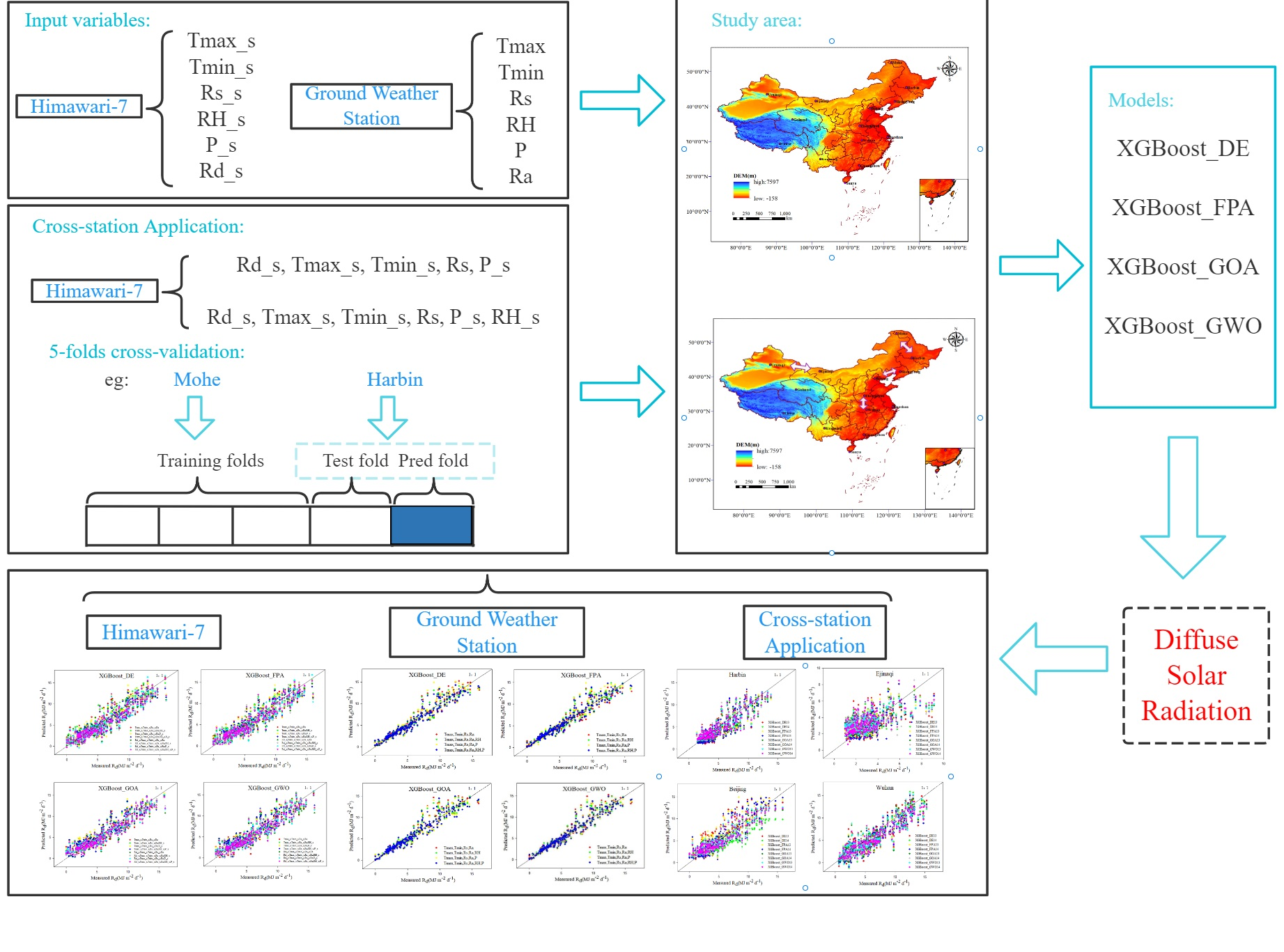
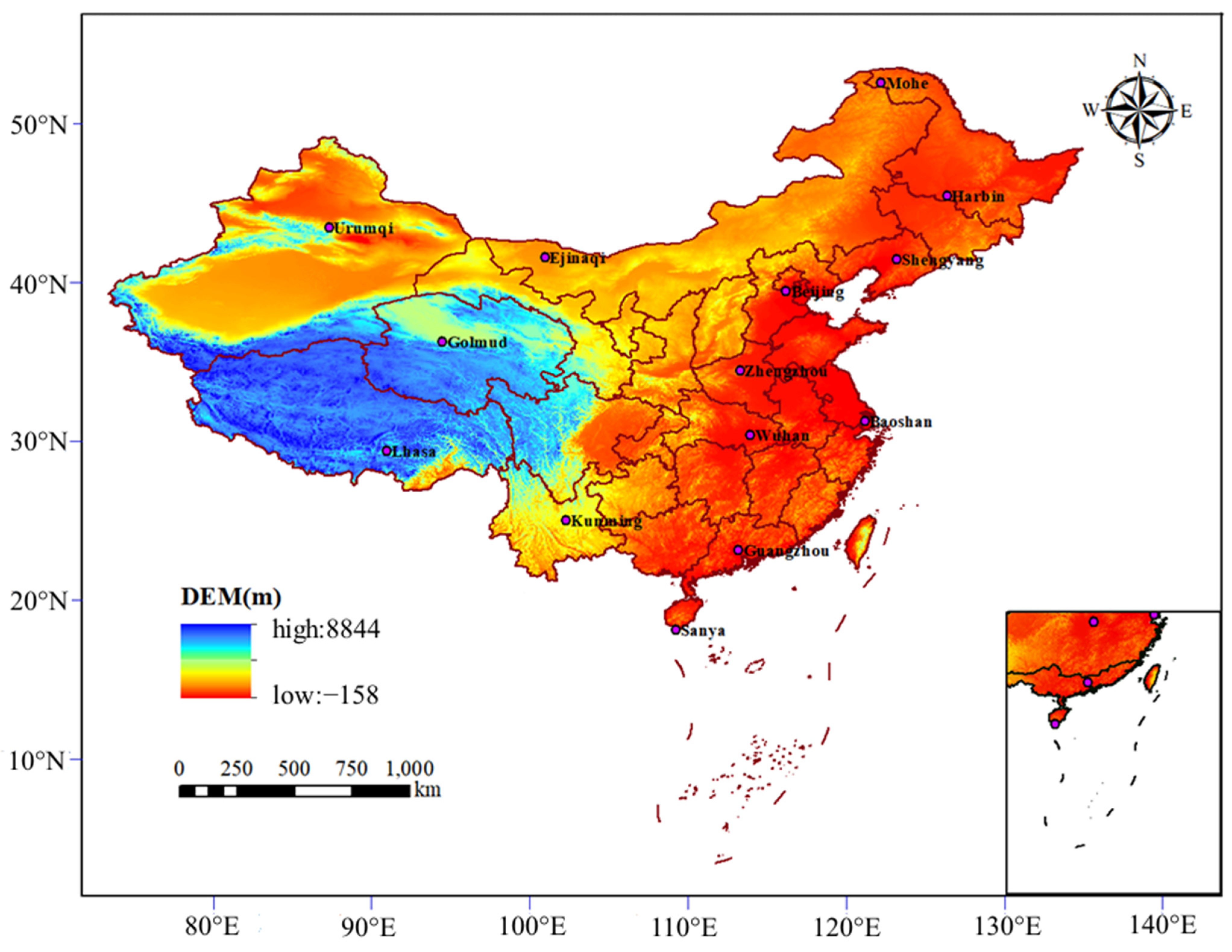
2.1. Study Area and Meteorological Data

2.1.1. Himawari-7 Data

The data of Himawari-7 from 2011 to 2015 at 14 stations with Rd measurement capabilities in mainland China were downloaded from the NSRDB (Figure 1) [17,18]. The meteorological data obtained included maximum/minimum temperature (Tmax_s/Tmin_s), relative humidity (RH_s), precipitation (P_s), solar horizontal total radiation (Rs_s), and solar diffuse radiation (Rd_s). The detailed geographic locations and satellite weather information for the 14 stations are shown in Table 1.

2.1.2. Ground Weather Stations Data

Some meteorological factors from 14 ground weather stations in mainland China were collected, including maximum/minimum temperature (Tmax/Tmin), relative humidity (RH), solar radiation (Rs), precipitation (P), and diffuse solar radiation (Rd). Daily extraterrestrial radiation (Ra) was calculated at latitude and each day of the year [19]. Table 1 showed the detailed geographical location and data of the selected stations, including the average values of meteorological factors obtained from 14 ground weather stations in 2011–2015. Each station has an average of more than 400 rows of data missing. Incomplete meteorological data were deleted during data processing.

2.2. Extreme Gradient Boosting

XGBoost was proposed by Chen et al. [20]. Through additional training to avoid overfitting, XGBoost integrates many weak learners and develops a strong learner, which is essentially a kind of boosting algorithm for ensemble learning in supervised learning. The objective function of XGBoost is expressed as the sum of the loss function and the regularization term. A smaller loss function indicates better model fitting effect, while a smaller regularization term indicates a lower model complexity. Similar to the traditional model, XGBoost uses residuals. Its algorithm utilizes split data in the data set to model separately [21], and unlike traditional, this is also a parameter-based algorithm. When the model is dealing with classification or regression problems, the model does not need to change the determined parameters. XGBoost has higher accuracy and greater flexibility. It adds regular terms to the objective function to prevent overfitting, which is one of the characteristics of XGBoost that is superior to traditional GBDT. However, it needs to traverse the data set in the process of node splitting. The pre-sorting process has high space complexity and consumes a lot of memory. The expressions are as follows:
f i ( t ) = k = 1 t f k ( x i ) = f i ( t 1 ) + f t ( x i )
where fi(t) is the simulation result of sample i after the t-th iteration, and fi(t−1) is the simulation result of step t − 1.
The accuracy of the model depends on the variance and deviation of the model, where the deviation is related to the loss function. In order to reduce the variance of the model and prevent overfitting, the regularization term needs to be added to the objective function. Therefore, the objective function consists of a loss function and a regularization term, which is defined as follows:
L = i = 1 n l ( y i , y i ¯ )
O b j = i = 1 n l ( y i , y i ¯ ) + i = 1 t Ω ( f i )
where L is the loss function, n is the number of samples, Obj is the objective function, and Ω is the sum of the complexity of all trees. Further computational programs and more information about XGBoost can be found in Chen’s research [22].

2.3. Heuristic Algorithms

2.3.1. Differential Evolution (DE) Algorithm

First proposed by Storn and Price [23], the DE algorithm is a kind of evolutionary algorithm that is extensively used in data mining, pattern recognition, electromagnetics, and other fields, owing to the simple structure and strong robustness thereof [24]. The optimization of DE algorithm firstly is to use floating point vector encoding to generate individuals, and select two individuals to generate a difference vector. Secondly, sum the difference vector generated in the previous step with another individual to generate an experimental individual; then, operate the individual generated by the previous generation and the experimental individual to generate a new generation of individuals; finally, choose the most suitable individual between the two generations to enter the next generation. The core idea of the DE algorithm is to use mutation and crossover operation to generate a test population and evaluate the fitness, and then compare the original population and test population one by one through the selection mechanism of greedy thought, and select the next generation. The DE algorithm has the advantages of simple operation, less controllable parameters, fast convergence speed, and strong global search ability, but it inevitably has the problem of stagnation when optimizing complex problems such as high dimension, multi-peak and multi-objective problems. The specific steps and expressions are as follows:
(1)
Initialization population
x i , j ( 0 ) = x i , j L + r a n d ( 0 , 1 ) ( x i , j U x i , j L )
where xi,jL and xi,jU denote the upper and lower bounds of dimension j, respectively, and rand(0,1) denotes the random number on the interval [0, 1].
(2)
Variation
The DE algorithm realizes individual mutation through differentiation strategy. The common differential strategy is to randomly select two different individuals in the population, and synthesize the vector with the individual to be mutated after the vector difference is scaled.
V i ( g + 1 ) = X r 1 ( g ) + F ( X r 2 ( g ) X r 3 ( g ) )
where r1, r2 and r3 are three random numbers in the interval [1, NP], F is the scaling factor, and g is the g-th generation.
(3)
Crossover
The purpose of crossover operation is to randomly select individuals.
U i , j ( g + 1 ) = V i , j ( g + 1 ) i f r a n d ( 0 , 1 ) C R x i , j ( g ) o t h e r w i s e
where CR is the crossover probability, which generates new individuals according to different probabilities.
(4)
Selection
DE algorithm selects the better individual as the new individual.
X i ( g + 1 ) = U i ( g + 1 ) i f f ( U i ( g + 1 ) ) f ( X i ( g ) ) X i ( g )
Further details about the differential evolution algorithm can be found in Storn and Price’s research [23].

2.3.2. Flower Pollination Algorithm (FPA)

The flower pollination algorithm (FPA) is a new meta-heuristic swarm intelligence optimization algorithm proposed by Yang [25]. The basic concept of the FPA was derived from the simulation of self-pollination and cross-pollination of flowers in nature. The algorithm is more effective than the genetic algorithm, and the convergence speed of the FPA is almost exponential. The algorithm follows the following four standardization principles: (1) during cross-pollination, the pollinator performs Lévy flight (long-distance movement), which is mapped to a global search process; (2) self-pollination is considered to be a local search process; (3) the stability of flowers can be regarded as the ratio of reproduction probability and similarity of two flowers during pollination; (4) the change of pollination method is controlled by switching probability p(p ∈ [0, 1]), that is, when random number “rand” < p, self-pollination is executed; otherwise, cross-pollination is executed. The algorithm imitates two mechanisms of natural flower pollination. Owing to the reliance on pollinators to spread pollen remotely, cross-pollination corresponds to a global search process, while self-pollination corresponds to the local search process due to the close distance in the physical position of pollination. A switching probability p(p ∈ [0, 1]) is introduced to weigh the ratio between the two search processes. The FPA is simple in theory and easy to implement, but there are still problems such as low convergence accuracy and sensitivity to dimensions. The expressions are as follows:
(1)
Cross-pollination formula:
X i t + 1 = X i t + L ( X i t g t )
where Xit denotes the i-th solution of the t-th generation respectively; gt is the t-th generation optimal solution; L is the step length.
(2)
Self-pollination formula:
The design idea of self-pollination algorithm is to simulate the close pollination between flowers of the same species in nature. The mathematical description is as follows:
X i t + 1 = X i t + ε ( X j t X k t )
where ε ∈ [0, 1] denotes the random number, Xjt and Xkt denote the j-th and k-th solutions in the t-th population, respectively. Further details about the flower pollination algorithm can be found in Yang’s research [25].

2.3.3. Grasshopper Optimization Algorithm (GOA)

The grasshopper optimization algorithm (GOA) is a swarm intelligence optimization algorithm proposed by Saremi et al. [26]. Similar to most other intelligence optimization algorithms, the GOA ensures that the algorithm can effectively search globally and avoid stopping at local optimum in both exploration and development. The life cycle of grasshoppers is primarily divided into two stages: larvae and adults. The main feature of the larvae stage is that grasshoppers move slowly in a small range, while in the adult stage, grasshoppers have strong hind legs and are good at jumping, being able to move long distances quickly. The exploration process of the GOA is equivalent to the adult stage, and the development process is equivalent to the larval stage. Looking for food sources is another main feature of the grasshopper population, with a food source being equivalent to the optimal solution, and the search for food being the process of finding the optimal solution. The GOA is stable and has good local search ability. However, its convergence speed is not fast. Since each individual accumulates other individuals except itself, the new position difference between individuals is small, and the locusts are easy to fall into local optimum in group aggregation. The expressions are as follows:
X i d = c j = 1 j i N c u b d l b d 2 s x j d x i d x j x i d i j + T d ¯
where Xid is the position of the i-th locust in the d-th dimension; ubd and lbd are the upper and lower bounds of the variable of the i-th locust in the d-th dimension; t is the target position of locust swarm.
c = c max t c max c min T max
where t represents the current number of iterations, Tmax is the maximum number of iterations, cmax and cmin are the maximum and minimum values of parameter c, respectively. Further details about the GOA can be found in Saremi’s research [26].

2.3.4. Gray Wolf Optimizer (GWO) Algorithm

Inspired by the predation activities of gray wolves, the gray wolf optimization (GWO) algorithm is a swarm intelligence optimization algorithm proposed by Mirjalili et al. [27]. The algorithm has the characteristics of strong convergence performance and easy implementation. Gray wolves strictly abide by a social dominance hierarchy. When designing a GWO algorithm, the gray wolf social hierarchy model needs to be firstly constructed, the fitness of each individual needs to be calculated, and the three gray wolves with the best fitness need to be placed on the higher level in turn. Gray wolves approach prey when searching, but gray wolves cannot determine the exact location of prey. The higher-level gray wolves are assumed to have stronger ability to obtain location information about their prey than lower-level ones for simulating the hunting behavior of gray wolves. Therefore, in each iteration process, several optimal gray wolves are kept, and the locations of other gray wolves are updated according to their location information. Compared with other algorithms, the optimization process of the GWO algorithm is faster. However, the GWO algorithm is a heuristic optimization algorithm, and the optimal solution is only close to the original optimal solution, not the real optimal solution of the problem. The expressions are as follows:
D = C X p t X t
X t + 1 = X p t A D
Equation (11) represents the distance between the individual and the prey, and Equation (12) is the position update formula of the gray wolf. Where t is the current number of iterations, Xp and X are the position vectors of prey and gray wolf, respectively, and A and C are the coefficient vectors. The calculation formulas are as follows:
A = 2 a r 1 a
C = 2 r 2
where a is the convergence factor. As the number of iterations decreases linearly from 2 to 0, r1 and r2 are random numbers in the interval [0, 1].
After the gray wolf recognizes the location of the prey, β and δ, led by α, guide the wolves to surround the prey. The expression is as follows:
D α = C 1 X α X D β = C 2 X β X D δ = C 3 X δ X
where Dα, Dβ and Dδ represent the distance between α, β and δ and other individuals, respectively; Xα, Xβ and Xδ denote the current positions α, β and δ, respectively. C1, C2 and C3 are random vectors, and X is the current position of the gray wolf.
X 1 = X α A 1 D α X 2 = X β A 2 D β X 3 = X δ A 3 D δ
X t + 1 = X 1 + X 2 + X 3 3
Equation (15) defines the step length and direction of ω individuals in the wolf pack towards α, β and δ, respectively. Equation (16) defines the final position ω. More details about the GWO algorithm can be found in Mirjalili’s research [27].

2.4. Input Combinations Based on Satellite and Ground Weather Station Data

Twelve meteorological environment variable input combinations of four coupling models were used to evaluate the effects of various input factors on Rd prediction: (1) eight combinations of input parameters were set based on satellite data (see Table 2); and (2) four combinations of input parameters were set based on ground weather station data (see Table 3). The K-fold cross-validation method was used for all the data obtained in the modeling process. The first three fifths (2011–2013) of these data were used to train these models, and the last two fifths (2014 and 2015) were used to test and verify these models.
XGBoost_DE1-8 represents the coupling model with combined S1-S8 inputs based on satellite data (see Table 2). XGBoost_DE9-12 represents the coupling model with combined L1-L4 input based on ground weather station data (see Table 3), and the symbolic meaning of others are the same as above.

2.5. Input Combinations Based on Cross-Station Application

According to the location of 14 stations, the relatively close stations were divided into pairs to test and verify the model of the adjacent stations based on satellite data of the target station. On the basis of satellite data, two sets of optimal-simulated combinations (see Table 4) were selected for cross-station application and four sets of stations with the highest data accuracy and optimal model performance were presented.

2.6. Statistical Indicators

The performance evaluation of four coupled models for simulation of the level of daily Rd was based on four widely adopted statistical indicators, including MAE, MBE, RMSE, and R2. RMSE reflects the overall estimation accuracy of the model, and R2 represents the percentage of data that the model can describe. MAE is used to describe the average deviation degree of each point, and MBE reflects the positive and negative deviation of the model. The formula of the statistical indicators could be denoted below:
MAE = 1 t i = 1 t X i , m X i , e
MBE = 1 t i = 1 t ( X i , m X i , e )
RMSE = 1 t i = 1 t ( X i , m X i , e ) 2
R 2 = [ i = 1 t ( X i , e X i , e ¯ ) ( X i , m X i , m ¯ ) ] 2 i = 1 t ( X i , e X i , e ¯ ) 2 i = 1 t ( X i , m X i , m ¯ ) 2
where Xi,m, Xi,e, Xi,m, Xi,e and t are the measured value of Rd, the simulated value of Rd, the average measured value of Rd, the average simulated value of Rd, and the data sample size, respectively. Higher R2 (close to 1) and lower MAE, MBE, and RMSE (close to 0) indicate better model fit and higher model performance.

3. Results

3.1. Accuracy Assessment of Diffuse Solar Radiation Data from Satellites

The Rd_s values of 14 stations in mainland China were obtained from Himawari-7 data, and the satellite measurements were statistically analyzed with the ground weather station measurements of the corresponding stations (see Table 5). During the validation period, an observation can be made from Table 5 that the RMSE and MAE of Harbin station were the lowest, being 1.741 MJ·m−2·d−1 and 1.196 MJ·m−2·d−1, respectively. The R2 of Lhasa station was the highest, being 0.81, and the MBE of Beijing station was the lowest, being 0.201 MJ·m−2·d−1. Compared with the other 12 stations, the satellite Rd data of Harbin and Beijing stations were more accurate. The average RMSE, MAE, and MBE values were 41.1%, 50.4%, and 57.8% lower, respectively, than the other stations, and the average R2 was 32.4% higher. In general, only a small number of stations could obtain a higher data accuracy by using Rd_s obtained by Himawari-7 data. The accuracy of Himawari-7 data at most stations was low and the error was large. Among them, the accuracy of satellite measurements of Rd_s in Urumqi, Guangzhou, and Sanya stations is significantly different from that of other stations. This may be due to the thickness of clouds at these stations and the changes of aerosols and water vapor on sunny days. There are difficulties in obtaining the ideal effect in practical application, and improvements are needed. This section analyzed and evaluated the accuracy of the Rd and measured values of 14 stations measured by Himawari-7, and these data were used for comparison with the simulation results of the tree-based coupling model in the following sections.

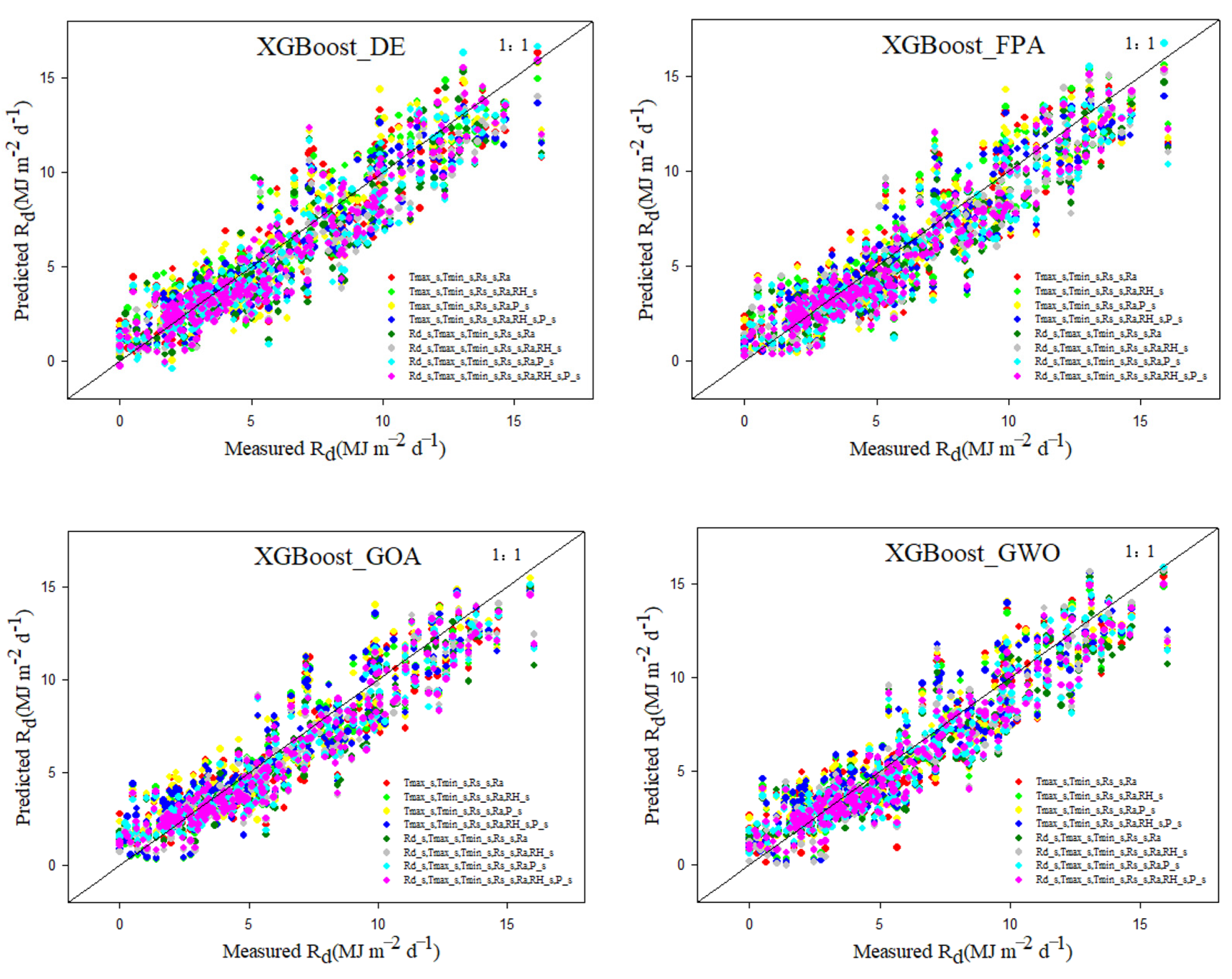
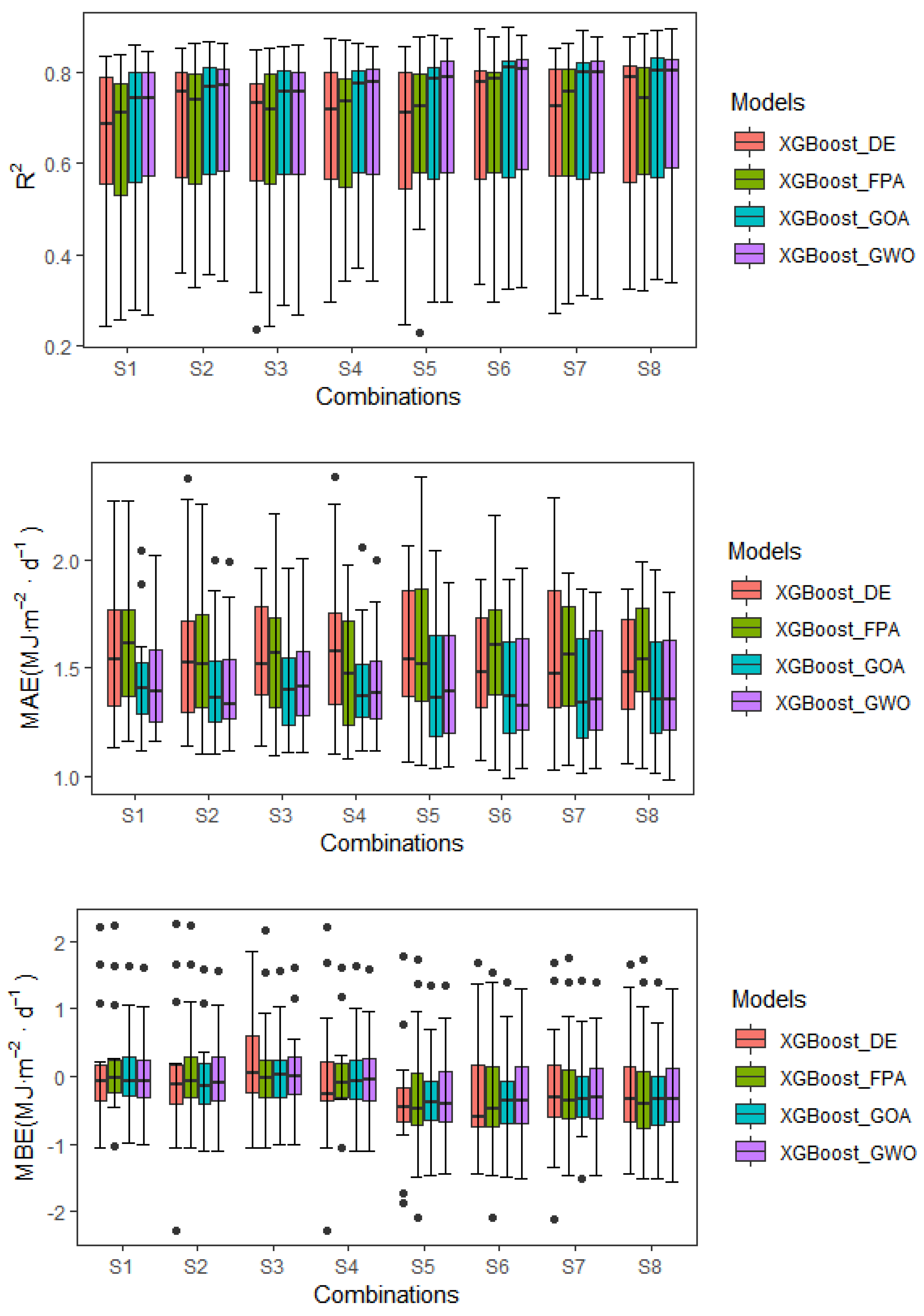
3.2. Model Performance Based on Himawari-7 Data

Four optimization algorithms (DE, FPA, GOA, and GWO) were used for coupling with the XGBoost model, so as to make better use of satellite data and improve the accuracy. Seven different parameters were selected: Tmax_s, Tmin_s, Rs_s, Rd_s, P_s, RH_s, and Ra. The parameters were divided into eight different input combinations to drive the four aforementioned coupling models (see Table 2). Based on satellite data of 14 stations, the Rd was predicted. The statistical summary of the verification period is shown in Table 6.
An observation can be made from the table that the four coupling models exhibited different accuracies under the input of different parameter combinations. Most models had MBE values less than 0 at most stations, so the simulation of Rd was generally underestimated. The RMSE, R2, and MAE values of the XGBoost_DE model were 1.948–2.11 MJ·m−2·d−1, 0.652–0.692, and 1.484–1.618 MJ·m−2·d−1, respectively. The RMSE, R2, and MAE values of the XGBoost_FPA model were 1.97–2.112 MJ·m−2·d−1, 0.642–0.682, and 1.493–1.607 MJ·m−2·d−1, respectively. The accuracy fluctuation of the XGBoost_DE model was the largest, followed by XGBoost_FPA model, while the accuracy fluctuations of the XGBoost_GOA and XGBoost_GWO model were small and considerably close.
The XGBoost_GOA model performed most optimally in simulating Rd based on satellite data, with RMSE and MAE values of 1.874 MJ·m−2·d−1 and 1.422 MJ·m−2·d−1, respectively. The XGBoost_DE model exhibited worse performance than the other three models, with RMSE and MAE values of 2.039 MJ·m−2·d−1 and 1.556 MJ·m−2·d−1, respectively. The analytical results reveal that the XGBoost_GOA model exhibited better performance. Scatter plots were used to present the simulated and measured values of the models for the Beijing station (Figure 2), so as to better compare the simulation performance of the XGBoost_DE, XGBoost_FPA, XGBoost_GOA, and XGBoost_GWO coupling models for Rd. As Figure 2 illustrates, the four coupling models showed high accuracy in simulating Rd. Among the four, the XGBoost_GOA model showed the most reliable estimation trend, and the dispersion level of the scatter was markedly lower than that of the XGBoost_DE and XGBoost_FPA model, and slightly lower than XGBoost_GWO model.
In order to explore whether relative humidity, precipitation, and satellite-measured Rd were dominant factors in simulating Rd, eight combinations were set up to respectively drive the model. Table 6 shows that the addition of P_s and RH_s could improve the simulation accuracy of Rd. Taking XGBoost_GOA model as an example, MBE, S1, S3, and S4 were used as input to obtain a smaller positive value, while the four groups of S5–S8 were significantly underestimated, and MBE was less than −0.15 MJ·m−2·d−1. In terms of RMSE and MAE, the model performed best when S8 was used as input, and the values were 1.856 MJ·m−2·d−1 and 1.409 MJ·m−2·d−1, respectively. When S1 was used as input, the model performed worst, with RMSE and MAE values of 1.905 MJ·m−2·d−1 and 1.451 MJ·m−2·d−1, respectively. As such, based on temperature, solar radiation, Rd, relative humidity, and precipitation, the XGBoost_GOA model was more accurate than the XGBoost_GOA model in terms of temperature and solar radiation. For the XGBoost_FPA model, when S7 was used as input, the RMSE, MAE, and MBE values of the model were better than those of the model when S8 was input, with differences of 0.27%, 0.35%, and 14.2%, respectively. For the XGBoost_DE model, in terms of R2, when S6 was used as input, R2 was the highest, being 0.692, but performed poorly in terms of MBE, being −0.198 MJ·m−2·d−1, second only to S7, which showed a serious underestimation of the model. With S2 as the input, the MBE was optimal at 0.011 MJ·m−2·d−1. For the XGBoost_GWO model, when S2 was used as input, the model performed optimally in terms of RMSE and MBE, which were 1.848 MJ·m−2·d−1 and 0.015 MJ·m−2·d−1, respectively, and there was no obvious overestimation. In terms of R2, the model performance was second only to S6 and S8, thereby demonstrating that the accuracy of the XGBoost_GWO model simulation and the Rd value measured by the satellite were less significant than the other three models under the input of the model. The aforementioned analysis results show that precipitation was more significant than relative humidity in simulating Rd using the XGBoost_FPA model. For the XGBoost_FPA and XGBoost_GOA models, the Rd values measured by satellites were more significant than those of the other two models. Figure 2 clearly illustrates the different effects of different factors’ inputs on the accuracy of these four models for simulating Rd. For XGBoost_DE and XGBoost_GOA model, the first seven combinations had higher errors, and the model input S8 (Rd_s, Tmax_s, Tmin_s, Rs_s, Ra, and RH_s, P_s) could produce higher simulation accuracy.
Boxplots were used to demonstrate the differences between the four coupled models for simulating Rd based on the Himawari-7 data at 14 stations in mainland China (Figure 3). Figure 3 shows that the abnormal values detected by the four combinations of S5–S8 were less than those of S1–S4. In terms of RMSE, the levels of the XGBoost_GOA and XGBoost_GWO model outperformed others. In terms of R2, the XGBoost_GOA model had better effect than the XGBoost_GWO model. In the case of input S1–S4, the dispersion degrees of the XGBoost_DE and XGBoost_FPA model simulation values were higher, while the dispersion degree of the XGBoost_GOA model simulation value was the lowest. As Figure 3 clearly shows, the simulation values of the XGBoost_GOA model were concentrated and showed high simulation levels in S3–S8. Although XGBoost_DE performed well in terms of the MBE values in S7–S8, the average simulation level was markedly lower than others.
In general, the XGBoost_GOA model performed optimally in the verification period, and Rd_s had the most remarkable effect on the performance of these models. Due to the limited number of research stations and the large span of the climate zone, the accuracy of the model based on satellite data to simulate the level of Rd was not high. Thus, attempts were made to investigate the performance of four coupling models to simulate Rd based on ground weather station data of the same 14 stations, and to compare the accuracy differences with the satellite data model.
Table 6. Statistical results of the XGBoost_DE, XGBoost_FPA, XGBoost_GOA, and XGBoost_GWO models for Rd prediction with eight combinations based on satellite data.
ModelsCombinations/Statistical IndicatorsRMSER2MAEMBE
XGBoost_DE1-8S12.084 0.652 1.577 0.164
S22.094 0.688 1.600 0.011
S32.019 0.652 1.553 0.215
S42.110 0.673 1.618 −0.033
S52.058 0.654 1.563 −0.383
S61.970 0.6921.499 −0.198
S72.033 0.670 1.554 −0.186
S81.9480.686 1.484−0.120
XGBoost_FPA1-8S12.112 0.642 1.607 0.205
S22.032 0.673 1.548 0.195
S32.040 0.660 1.560 0.182
S41.9700.673 1.4930.047
S52.081 0.669 1.586 −0.261
S62.078 0.6821.564 −0.271
S72.016 0.678 1.531 −0.142
S82.022 0.680 1.536 −0.166
XGBoost_GOA1-8S11.9050.6781.4510.038
S21.8580.6991.416−0.042
S31.8780.6861.4330.025
S41.8630.6961.4180.022
S51.8890.6951.425−0.263
S61.8720.7061.41−0.236
S71.8710.7031.413−0.193
S81.8560.7091.409−0.24
XGBoost_GWO1-8S11.9050.681.4570.035
S21.8480.7011.4160.015
S31.8890.6851.4470.069
S41.8530.6961.4210.029
S51.9020.6961.434−0.225
S61.8580.7131.409−0.239
S71.8880.7011.426−0.193
S81.8510.7131.402−0.237
Figure 2. Scatter plots of Rd predicted by the coupling models based on Himawari-7 data in Beijing.
Remotesensing 15 01885 g002
Figure 3. Boxplot of statistical indicators for the prediction of Rd by the coupling model based on Himawari-7 data.
Remotesensing 15 01885 g003aRemotesensing 15 01885 g003b

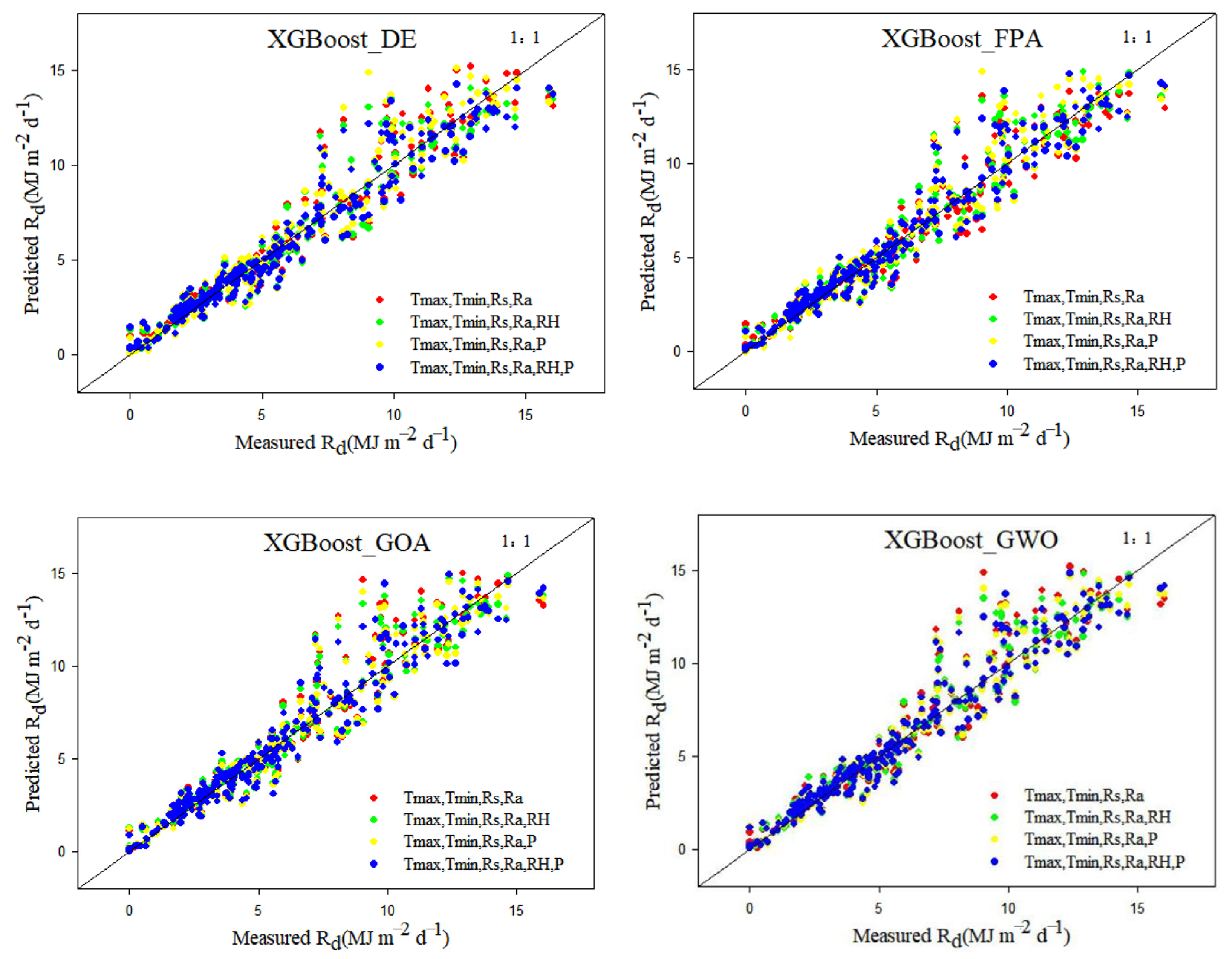
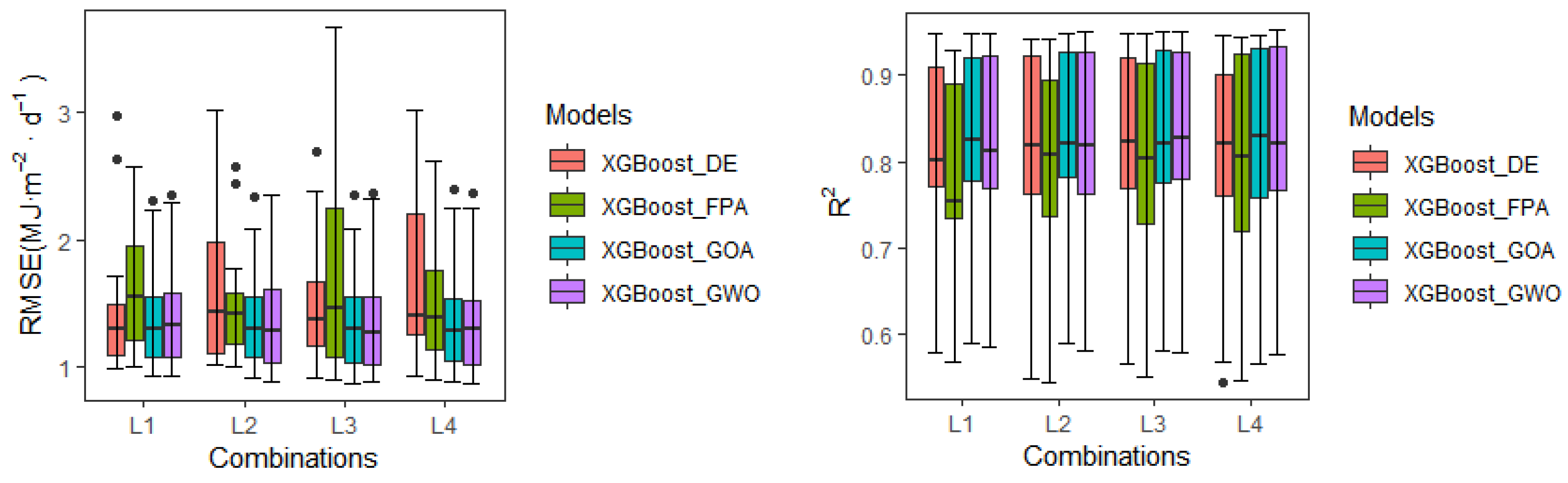
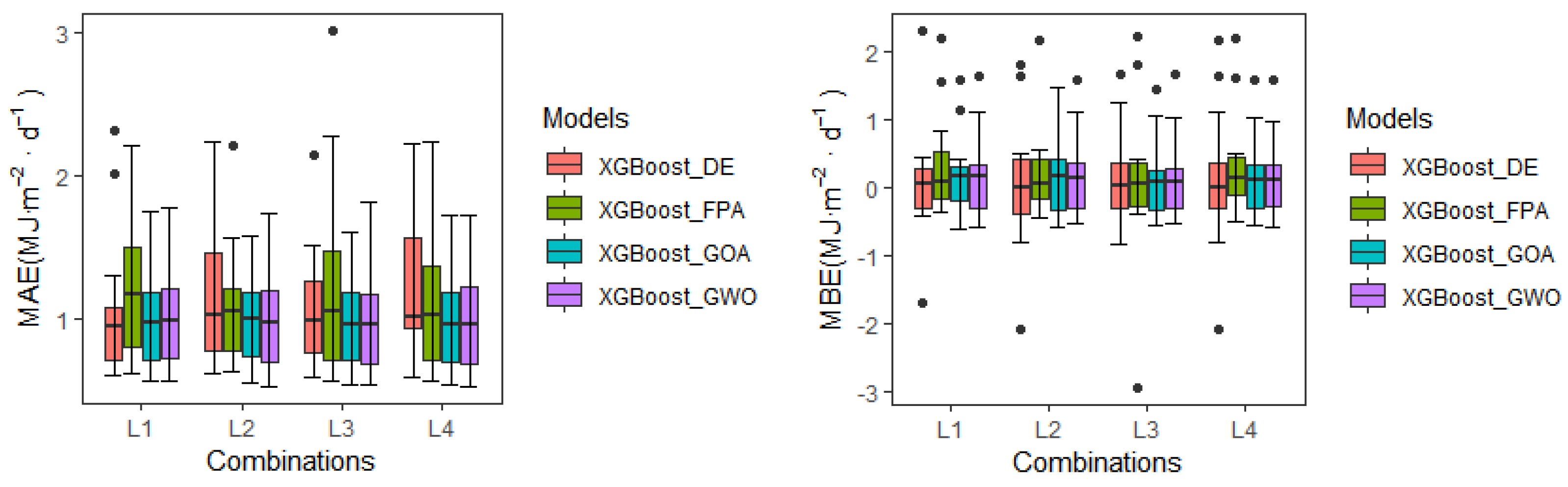
3.3. Model Performance Based on Ground Weather Station Data

The factors obtained from the ground weather station, namely Tmax, Tmin, Rs, RH, and P, were applied to simulate the Rd. The five parameters were divided into four groups (see Table 3) and input into four coupling models. The statistical indicators of the simulated Rd were contrasted with the statistical indicators based on Himawari-7 data simulation. Based on the observation stations and satellite data, the significance of parameters from observation station to the performance of these models’ simulation and the differences in the performance of the simulated Rd were evaluated (see Table 7). An observation can be made from the table that in the case of inputting the same meteorological factors, the XGBoost_GOA model (mean RMSE = 1.381 MJ·m−2·d−1, R2 = 0.832, MAE = 0.993 MJ·m−2·d−1, MBE = 0.162 MJ·m−2·d−1) was significantly better than others (mean RMSE = 1.387–1.589 MJ·m−2·d−1, R2 = 0.799–0.831, MAE = 0.996–1.167 MJ·m−2·d−1, MBE = 0.1–0.235 MJ·m−2·d−1). Scatter plots of the four coupling models were drawn based on the data observed in Beijing station (Figure 4). Figure 4 showed that the capability of the XGBoost_GOA model and the XGBoost_GWO model exhibited a similar simulation trend, being closer to the fitting line and more evenly distributed than the other two models. The dispersion degree of each model in the case of inputting the L4 combination was lower than the dispersion degrees of the other three combinations.
Table 7 shows that the accuracy of each model was different when different parameter combinations were input. For the XGBoost_DE model, the model showed the optimal simulation level in the case of inputting the L1 combination. Compared with the L2-L4 combinations, the RMSE and MAE values were reduced by 0.2–11.1%, 1–13.4%, and R2 increased by 0.8–1.6%. For the XGBoost_FPA model, when the L2 combination was input, the RMSE and MAE values of the model were the lowest, being 1.495 MJ·m−2·d−1 and 1.097 MJ·m−2·d−1, respectively. For the XGBoost_GOA model, the four input effects of the model were significantly better than the XGBoost_DE and XGBoost_FPA models. The accuracy performance was as follows: L3 > L4 > L1 > L2. The L3 input combination performed most optimally among all models and combinations, with RMSE, R2, MAE, and MBE values of 1.362 MJ·m−2·d−1, 0.834, 0.979 MJ·m−2·d−1, and 0.129 MJ·m−2·d−1, respectively. For the XGBoost_GWO model, the relatively complex parameter combination of L4 had the optimal model simulation effect (RMSE = 1.374 MJ·m−2·d−1, MAE = 0.988 MJ·m−2·d−1), which was slightly better than the L3 combination (RMSE = 1.375 MJ·m−2·d−1, MAE = 0.99 MJ·m−2·d−1). From the aforementioned analysis, an observation can be made that relative humidity and precipitation had an adverse effect on the XGBoost_DE model. Relative humidity can refine the ability of the XGBoost_FPA model. Precipitation has a positive effect on the XGBoost_GOA model, and the co-input of such meteorological factors significantly refined the performance of the XGBoost_GWO model.
The statistical indicators of the model simulation values based on ground weather station data are shown in Figure 5. An observation can be made from the boxplots that the data of the XGBoost_DE model fluctuated greatly with the input combinations of L2 and L4, and the data of the XGBoost_FPA model fluctuated greatly with the input combinations of L1 and L3. Overall, the RMSE values of the XGBoost_GOA and XGBoost_GWO model were markedly lower than those of others. As the complexity of the input meteorological factors increased, the data for the XGBoost_GWO model became more concentrated. As such, the XGBoost_GOA model and the XGBoost_GWO model were superior to others in simulating Rd, thereby revealing the significance of the input of two meteorological factors, relative humidity and precipitation, to the XGBoost_GWO model simulation.
Table 7. Statistical results of the XGBoost_DE, XGBoost_FPA, XGBoost_GOA, and XGBoost_GWO models for Rd prediction with four combinations based on ground weather stations data.
ModelsCombination/Statistical IndicatorsRMSER2MAEMBE
XGBoost_DE9-12L11.4780.8211.0700.057
L21.605 0.819 1.167 0.056
L31.480 0.814 1.082 0.148
L41.662 0.808 1.235 0.140
XGBoost_FPA9-12L11.643 0.777 1.215 0.321
L21.4950.800 1.0970.224
L31.695 0.8121.251 0.086
L41.523 0.808 1.104 0.310
XGBoost_GOA9-12L11.3900.8321.0050.186
L21.3920.8311.0000.162
L31.3620.8340.9790.129
L41.3780.8310.9890.170
XGBoost_GWO9-12L11.4080.8281.0100.178
L21.3930.8300.9970.173
L31.3750.8340.9900.158
L41.3740.8330.9880.159
Figure 4. Scatter plots of Rd predicted by the coupling models based on ground weather station data in Beijing.
Remotesensing 15 01885 g004
Figure 5. Boxplot of statistical indicators for the prediction of Rd by the coupling model based on ground weather station data.
Remotesensing 15 01885 g005aRemotesensing 15 01885 g005b

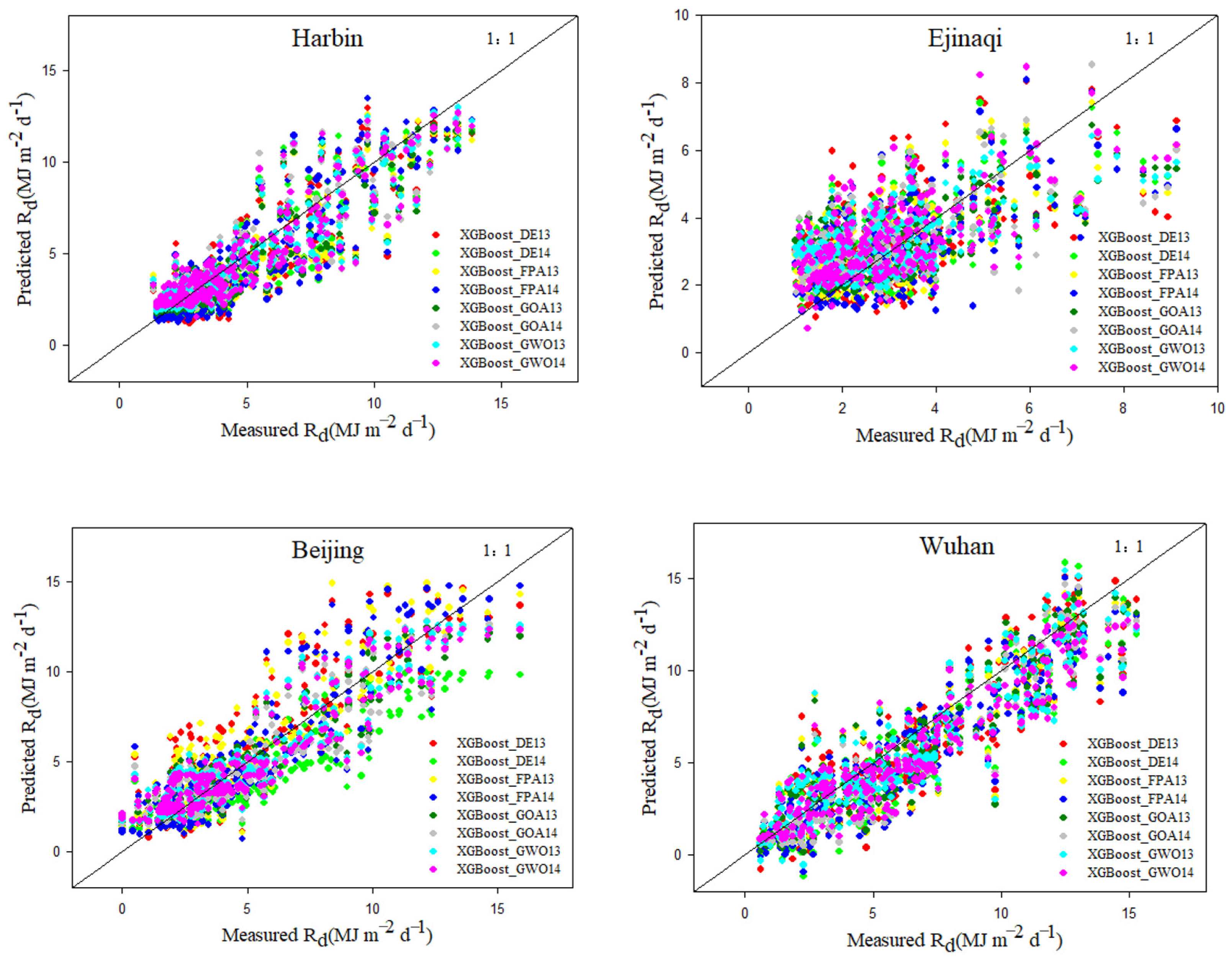
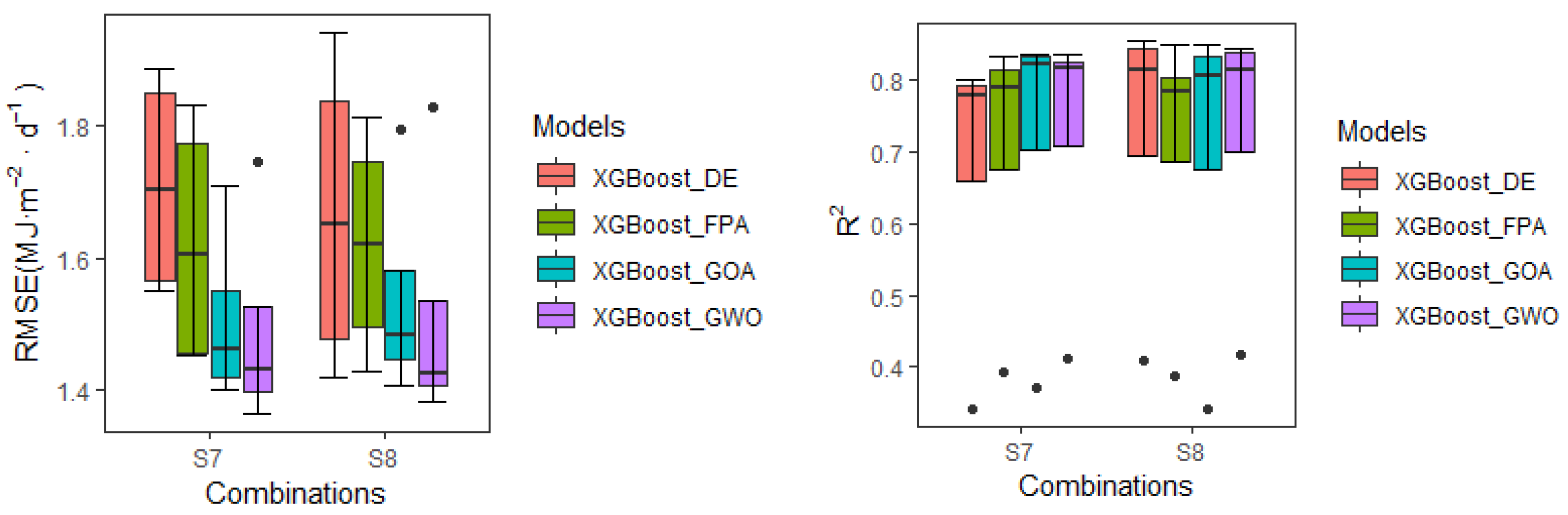
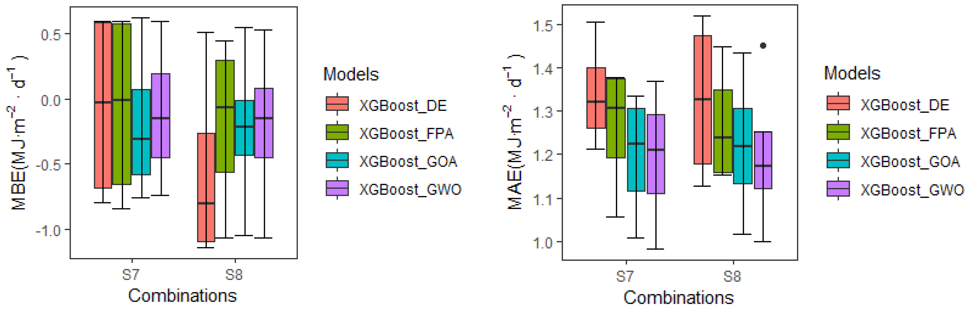
3.4. Model Performance Based on Cross-Station Application

When areas lacking basic data for simulating Rd were identified, such areas were replaced by data from adjacent regions that have the required data, which was described as “cross-station application”. In China and many developing countries, where local meteorological data are missing or insufficient, satellite data are often used to establish models for the simulation of Rd. However, in certain remote areas of China, ground meteorological data are often missing and there is a lack of full coverage of satellite remote sensing. In the traditional simulation of Rd values of a station, the ground weather station data of adjacent stations are often used. In the present study, the satellite data of adjacent stations were replaced to explore the universality of satellite remote sensing data in remote areas around the world. An assumption was made that there were four stations (Harbin, Ejinaqi, Beijing, and Wuhan stations) missing several significant data used to simulate Rd. Therefore, the meteorological data of one station were replaced with the Himawari-7 data obtained from the station closest to the four stations, and the four aforementioned coupling models were used to simulate the Rd. The Rd value of the station was simulated based on satellite data of the adjacent station (see Table 8).
As shown in Table 8, different station data adapted to different models. The XGBoost_GWO13 model performed optimally at Harbin and Beijing stations, and the RMSE values were 1.2–13.1% and 0.4–27.4% lower than the other models, respectively. The XGBoost_DE model and the XGBoost_FPA model exhibited resembling simulation level, but were obviously inferior to the XGBoost_GOA model and the XGBoost_GWO model. For Harbin station, the MAE, MBE, and RMSE values of the former were 13.5%, 6.4%, and 8.8% lower than the latter, respectively. The XGBoost_GOA model (average RMSE = 1.752 MJ·m−2·d−1) was only slightly better than the XGBoost_GWO model (average RMSE = 1.787 MJ·m−2·d−1) at the Wuhan station. Scatter plots were drawn of the Rd simulated using the four coupled models in cross-station application at these four stations (Figure 6). Figure 6 clearly illustrated that the scatter distribution of the model established at each station had a certain linear relationship. The scatter distribution at the Wuhan station was the most uniform, and the model showed the most accurate simulation trend. The dispersion degrees of the scatter plot at the Beijing and Harbin stations were slightly higher than that at the Wuhan station, while the scatter distribution at the Ejinaqi station deviated greatly from the fitting line. Further, the fitting degree of the XGBoost_GWO model was markedly higher than that of the others. In general, each model exhibited ideal results in cross-station applications, especially the XGBoost_GWO model. The simulation performance was the most optimal, and thus, use of the adjacent station data to replace the local station data in the absence of satellite data is feasible.
Different combinations used at different stations in the same model can also lead to differences in model simulation capabilities. Table 8 shows that at Harbin, Beijing, and Wuhan stations, the performance of these models’ input combination of S7 was better than that of the combination of S8. Taking Harbin station as an instance, the average RMSE of the former was 0.2 % lower than that of the latter, while at Ejinaqi station, the average RMSE of the former was 2.8 % higher than that of the latter. The XGBoost_DE model reveled the best simulation performance at Harbin, Ejinaqi, and Wuhan stations for the input combination of S8 (mean RMSE = 1.67 MJ·m−2·d−1, R2 = 0.64, MAE = 1.33 MJ·m−2·d−1, MBE = −0.29 MJ·m−2·d−1) compared with S7 (mean RMSE = 1.57 MJ·m−2·d−1, R2 = 0.68, MAE = 1.26 MJ·m−2·d−1, MBE = −0.37 MJ·m−2·d−1). At the four stations, the XGBoost_GOA model input combination of S7 was better than the input combination of S8. As such, increasing the input of RH_s reduced the simulation performance of the model, which could be attributed to the large difference in relative humidity caused by the excessive number of influencing factors, thereby reducing the accuracy of the data. Figure 7 shows the boxplots of the statistical indicators of these coupling models using the satellite data to detect the Rd values. In terms of RMSE, the accuracy levels of these models were as follows: XGBoost_GWO > XGBoost_GOA > XGBoost_FPA > XGBoost_DE. In terms of MBE, when the combination of S8 was input into the XGBoost_DE model, the model was significantly underestimated, which indicates that the accuracy of RH_s was insufficient, which made the model less stable.
In summary, the XGBoost_GWO13 model performed optimally in simulating Rd. The model is most suitable for cross-station applications at Harbin and Beijing stations, while the XGBoost_GOA13 model had better simulation performance at Wuhan station. In addition, the relative humidity obtained by the Himawari-7 satellite is not suitable for model simulations. In the present study, only a few groups of stations were adopted as representatives to prove the applicability of cross-station applications for simulating Rd. In the future, a more suitable model should be explored and established, higher-precision satellite remote sensing data should be used, and more groups of stations should be selected for cross-station applications, so as to estimate the level of each model to predict Rd values using satellite remote sensing data at stations in different climate zones.
Table 8. Statistical results of XGBoost_DE, XGBoost_FPA, XGBoost_GOA, and XGBoost_GWO models for simulating Rd in Mohe, Urumqi, Shengyang, and Zhengzhou stations based on satellite data at Harbin, Ejinaqi, Beijing, and Wuhan stations.
StationsModelsCombinations/Statistical IndicatorsRMSER2MAEMBE
HarbinXGBoost_DE13S71.5690.7891.211−0.651
XGBoost_DE14S81.4960.7901.129−0.526
XGBoost_FPA13S71.457 0.805 1.055 −0.599
XGBoost_FPA14S81.5160.7851.153−0.392
XGBoost_GOA13S71.4010.8101.009−0.520
XGBoost_GOA14S81.4070.7841.016−0.200
XGBoost_GWO13S71.3630.8070.982−0.357
XGBoost_GWO14S81.3800.7941.001−0.246
EjinaqiXGBoost_DE13S71.5510.3421.2780.593
XGBoost_DE14S81.4190.4101.1960.508
XGBoost_FPA13S71.4520.3931.2380.568
XGBoost_FPA14S81.4270.3891.1620.446
XGBoost_GOA13S71.4990.3721.2980.622
XGBoost_GOA14S81.5100.3421.2630.548
XGBoost_GWO13S71.4520.4131.2660.593
XGBoost_GWO14S81.4360.4181.1850.535
BeijingXGBoost_DE13S71.8390.7631.3650.589
XGBoost_DE14S81.9420.8371.519−1.144
XGBoost_FPA13S71.8310.7701.3760.600
XGBoost_FPA14S81.7250.7841.3160.247
XGBoost_GOA13S71.4240.8311.150−0.106
XGBoost_GOA14S81.4570.8251.173−0.226
XGBoost_GWO13S71.4090.8331.1530.061
XGBoost_GWO14S81.4150.8341.161−0.068
WuhanXGBoost_DE13S71.8860.7991.506−0.800
XGBoost_DE14S81.8040.8521.457−1.081
XGBoost_FPA13S71.7540.8311.372−0.844
XGBoost_FPA14S81.8150.8481.447−1.072
XGBoost_GOA13S71.7090.8331.334−0.756
XGBoost_GOA14S81.7950.8491.433−1.050
XGBoost_GWO13S71.7450.8221.369−0.744
XGBoost_GWO14S81.8290.8431.450−1.070
Figure 6. Scatter plot of Rd predicted by the coupling models based on Himawari-7 data at other stations in cross-station application.
Remotesensing 15 01885 g006
Figure 7. Boxplot of statistical indicators for the prediction of Rd predicted by the coupling models based on Himawari-7 data at other stations in cross-station application.
Remotesensing 15 01885 g007aRemotesensing 15 01885 g007b

4. Discussion

Rd is a significant parameter in the design of various solar devices, and various techniques have been developed due to the inconsistency of the frequencies at which Rd is measured [28,29]. Owing to scarce ground weather stations and uneven distribution of meteorological data in time and space, satellite remote sensing data are often used by researchers to simulate Rd due to the wide coverage and continuous advantages in time and space. As an example, for mapping with data from four ground weather stations in Thailand, Charuchittipan et al. [30] used data from the multi-functional transport satellite (Himawari-6) for 2006–2015 and the Himawari-8 satellite for 2016 to design a semi-empirical model for Rd estimation. The results revealed that the estimated values of the developed semi-empirical model agreed well with the measured values. To improve the empirical model of monthly and daily Rd in northern China, Feng et al. [31] used the aerosol optical depth measured by the MODIS satellite and the solar radiation measured by a ground weather station. The improved model was found to have improved the estimation accuracy of Rd compared with the existing model. Bakirci [32] compared the Rd value obtained from the NASR-SSE database with the Rd value calculated by the model in two cities in Turkey to examine the ability of these models. The statistical results revealed that the optimal model could maintain good prediction accuracy using the Rd value obtained from the NASA-SSE database. To evaluate the European Centre for Medium-Range Weather Prediction fifth-Generation Reanalysis (ERA5) data and JiEA Satellite Retrieval Centre (JiEA) for Rd in East Asia, Jiang et al. [33] used ground weather station measurements from 39 stations of the World Radiation Data Centre (WRDC) and the China Meteorological Administration. The results showed that JiEA was in good agreement with the measurements, while ERA5 significantly underestimated the Rd. Such research has indicated that satellite data had certain accuracy in simulating Rd. In the present study, four heuristic algorithms were proposed for optimizing the machine learning model and simulating Rd based on satellite data, with the aim of evaluating the performance of these models. An observation can be made from Figure 2 that the models based on Himawari-7 data revealed a good fitting trend, which was consistent with the research results.
In the condition of simulating Rd based on satellite data, the input of different meteorological factors had different effects on the model. The input of P_s was found to have a more significant improvement than RH_s when using the XGBoost_FPA model. Zhou et al. [34] revealed that the introduction of precipitation could efficiently improve the underestimation of Rd. In humid areas, the correlation between precipitation and Rd was stronger than that of relative humidity, and similar results were obtained in this study. Yang et al. [35] selected data from 17 stations from 2000 to 2017 to build 18 Rd models and found that models with a combination of relative humidity, air temperature, and two other parameters (clearness index and relative sunshine hours) performed optimally among all models, which is consistent with the discoveries of the present study that using the XGBoost_DE and XGBoost_GWO models with a combination of relative humidity as an input could improve model performance. There were few studies on the simulation of diffuse solar radiation using the same machine learning model and heuristic optimization algorithm as this study, but some researchers used similar techniques to simulate diffuse solar radiation. For example, Fan et al. [15] proposed three new hybrid support vector machines to simulate diffuse solar radiation. The results showed that the coupled models (i.e., SVM-WOA, SVM-PSO, and SVM-BAT) further improved the prediction accuracy compared with the SVM model, which indicated that the use of heuristic algorithms to optimize the machine learning model could significantly improve the prediction results. It confirmed the feasibility of the coupling model method in this study.
Since certain areas are outside the satellite radiation range, the corresponding meteorological data could not be obtained. However, use of the available satellite data of adjacent stations as the training set of the model to simulate local Rd has become a widely used and effective method [36,37,38,39]. In most prior studies, the method of cross-station application was used to estimate ET0, rather than Rd. For instance, Shiri et al. [40] collected meteorological data from the Basque Country (humid region) and Valencia Country (non-humid region) in Spain to train a neuro-fuzzy model. The results revealed that the GNF model successfully estimated the ET0 value in Iran. In this study, four coupling models were selected to conduct cross-station applications at four similar groups of stations, showing high simulation accuracy. The Rd values at four stations were also successfully estimated, which indicated that the cross-station application method was feasible in many fields including the direction of Rd.
In investigating Rd, most previous researchers used the data of ground weather stations, and there was a lack of significant meteorological factors. Therefore, the selection of satellite products with high accuracy of measurement data and the improvement of satellite data with low accuracy were used to promote the performance of the model, which is of considerable significance in the simulation of Rd. In this study, four coupling models were selected to input different parameter combinations to simulate Rd based on satellite data and meteorological data of 14 stations. At the same time, cross-station applications were conducted on four groups of stations in terms of Rd, in accordance with the experiences of previous researchers. The present study can provide certain reference value for exploring the performance of the four coupling models in the assessment of Rd and the regional applicability of cross-station applications in mainland China. In a follow-up study, better heuristic algorithms and models based on the data of other satellite products should be used to conduct cross-station applications in other countries with different climates to overcome the low accuracy of the meteorological parameters input in this study and the limited number of stations.

5. Conclusions

The performances of four coupled models (XGBoost_DE, XGBoost_FPA, XGBoost_GOA, and XGBoost_GWO) in simulating Rd based on satellite data and ground weather station data were evaluated, as well as the performances in terms of cross-station applications based on satellite data at four stations (Harbin-Mohe, Ejina-Urumqi, Beijing-Shenyang, and Wuhan-Zhengzhou).
The results show that: (1) the model based on Himawari-7 data was markedly promoted compared with the satellite original Rd data; (2) among the models based on satellite and ground weather station data, the XGBoost_GOA model performed optimally, slightly better than the XGBoost_GWO model, and the XGBoost_GWO model had the optimal simulation performance in cross-station application; and (3) in the case of satellite data, the input of P_s and Rd_s could improve the performance of the XGBoost_FPA and XGBoost_GWO models. In the case of ground weather station data, the input of relative humidity was beneficial for improving the performance of the XGBoost_FPA and XGBoost_GWO models, and the input of precipitation was beneficial for improving the performance of XGBoost_GOA model, both of which were not suitable for the input of the XGBoost_DE model.
The present study can contribute a scheme for the global prediction of Rd in the absence of ground weather station and satellite data. In future research, more parameters and different algorithms can be introduced to simulate Rd, and adjacent stations in the same climate zone can be selected for cross-station application to avoid the impact of regional differences on data integrity.

Author Contributions

Conceptualization, S.Z., L.W. and Y.X.; methodology, S.Z., L.W. and Y.X.; software, S.Z.; validation, S.Z., L.W. and Y.X.; formal analysis, S.Z. and X.L.; investigation, S.Z. and J.D.; resources, S.Z. and F.Z.; data curation, S.Z., Y.C. and Z.L.; writing—original draft preparation, S.Z.; writing—review and editing, S.Z., L.W. and Y.X.; visualization, S.Z.; supervision, S.Z.; project administration, L.W. and Y.X.; funding acquisition, L.W. and Y.X. All authors have read and agreed to the published version of the manuscript.

Funding

This research was funded by [Lifeng Wu] grant number [20212BDH80016].

Data Availability Statement

Himawari-7 satellite remote sensing data is located in the National Solar Radiation Database(https://nsrdb.nrel.gov/data-viewer).

Conflicts of Interest

The authors declare no conflict of interest.

Nomenclature

Variables
RaExtra-terrestrial solar radiation (MJ·m−2·d−1)
Tmaxmaximum temperature from weather station(°C)
Tminminimum temperature from weather station(°C)
Rsglobal solar radiation from weather station (MJ·m−2·d−1)
RHDaily average air relative humidity from weather station (%)
Pprecipitation from weather station(mm)
Tmax_smaximum temperature from satellite(°C)
Tmin_sminimum temperature from satellite(°C)
Rs_sglobal solar radiation from satellite (MJ·m−2·d−1)
Rd_sdiffuse solar radiation from satellite (MJ·m−2·d−1)
RH_sDaily average air relative humidity from satellite (%)
P_sprecipitation from satellite(mm)
Abbreviations
XGBoostExtreme gradient boosting
DEDifferential Evolution Algorithm
FPAFlower Pollination Algorithm
GOAGrasshopper Optimization Algorithm
GWOGrey Wolf Optimizer Algorithm
RMSEroot mean square error (MJ·m−2·d−1)
R2coefficient of determination
MAEmean absolute error (MJ·m−2·d−1)
MBEmean bias error (MJ·m−2·d−1)
NSRDBNational Solar radiation Database
ANNArtificial Neural Network
SVMSupport Vector Machine
FFAfirefly algorithm
CNQRcopula-base nonlinear quantile regression
RFRandom Forest
KNNK- Nearest Neighbor
PSOParticle Swarm Optimization
WOAWhale Optimization Algorithm
BATBat Algorithm
ET0reference evapotranspiration
GNFGeneralized Neuro-fuzzy

References

  1. Khosravi, A.; Koury, R.N.N.; Machado, L.; Pabon, J.J.G. Prediction of hourly solar radiation in Abu Musa Island using machine learning algorithms. J. Clean. Prod. 2018, 176, 63–75. [Google Scholar] [CrossRef]
  2. Jiang, Y. Estimation of monthly mean daily diffuse radiation in China. Appl. Energ. 2009, 86, 1458–1464. [Google Scholar] [CrossRef]
  3. Khorasanizadeh, H.; Mohammadi, K. Diffuse solar radiation on a horizontal surface: Reviewing and categorizing the empirical models. Renew. Sustain. Energy Rev. 2016, 53, 338–362. [Google Scholar] [CrossRef]
  4. Fan, J.; Chen, B.; Wu, L.; Zhang, F.; Lu, X.; Xiang, Y. Evaluation and development of temperature-based empirical models for estimating daily global solar radiation in humid regions. Energy 2018, 144, 903–914. [Google Scholar] [CrossRef]
  5. Aler, R.; Galván, I.M.; Ruiz-Arias, J.A.; Gueymard, C.A. Improving the separation of direct and diffuse solar radiation components using machine learning by gradient boosting. Sol. Energy 2017, 150, 558–569. [Google Scholar] [CrossRef]
  6. Liu, B.Y.; Jordan, R.C. The interrelationship and characteristic distribution of direct, diffuse and total solar radiation. Sol. Energy 1960, 4, 1–19. [Google Scholar] [CrossRef]
  7. Ali, K.H. Empirical Model for Estimating Global Solar and Diffuse Solar Radiations on Horizontal Surfaces. J. Energy Technol. Policy 2016, 6, 40–50. [Google Scholar]
  8. Sabzpooshani, M.; Mohammadi, K. Establishing new empirical models for predicting monthly mean horizontal diffuse solar radiation in city of Isfahan, Iran. Energy 2014, 69, 571–577. [Google Scholar] [CrossRef]
  9. Mohammed, O.W.; Yanling, G. Estimation of Diffuse Solar Radiation in the Region of Northern Sudan. Int. Energy J. 2016, 16, 163–172. [Google Scholar]
  10. Jiang, Y. Prediction of monthly mean daily diffuse solar radiation using artificial neural networks and comparison with other empirical models. Energ. Policy 2008, 36, 3833–3837. [Google Scholar] [CrossRef]
  11. Liu, Y.; Zhou, Y.; Chen, Y.; Wang, D.; Wang, Y.; Zhu, Y. Comparison of support vector machine and copula-based nonlinear quantile regression for estimating the daily diffuse solar radiation: A case study in China. Renew. Energ. 2020, 146, 1101–1112. [Google Scholar] [CrossRef]
  12. Husain, S.; Khan, U.A. Machine learning models to predict diffuse solar radiation based on diffuse fraction and diffusion coefficient models for humid-subtropical climatic zone of India. Clean. Eng. Technol. 2021, 5, 100262. [Google Scholar] [CrossRef]
  13. Karaveli, A.B.; Akinoglu, B.G. Comparisons and critical assessment of global and diffuse solar irradiation estimation methodologies. Int. J. Green Energy 2018, 15, 325–332. [Google Scholar] [CrossRef]
  14. Rusen, S.E.; Konuralp, A. Quality control of diffuse solar radiation component with satellite-based estimation methods. Renew. Energ. 2020, 145, 1772–1779. [Google Scholar] [CrossRef]
  15. Fan, J.; Wu, L.; Ma, X.; Zhou, H.; Zhang, F. Hybrid support vector machines with heuristic algorithms for prediction of daily diffuse solar radiation in air-polluted regions. Renew. Energ. 2020, 145, 2034–2045. [Google Scholar] [CrossRef]
  16. Ma, R.; Letu, H.; Yang, K.; Wang, T.; Shi, C.; Xu, J.; Shi, J.; Shi, C.; Chen, L. Estimation of Surface Shortwave Radiation From Himawari-8 Satellite Data Based on a Combination of Radiative Transfer and Deep Neural Network. IEEE Trans. Geosci. Remote 2020, 58, 5304–5316. [Google Scholar] [CrossRef]
  17. Dong, J.; Liu, X.; Huang, G.; Fan, J.; Wu, L.; Wu, J. Comparison of four bio-inspired algorithms to optimize KNEA for predicting monthly reference evapotranspiration in different climate zones of China. Comput. Electron. Agric. 2021, 186, 106211. [Google Scholar] [CrossRef]
  18. Dong, J.; Wu, L.; Liu, X.; Fan, C.; Leng, M.; Yang, Q. Simulation of Daily Diffuse Solar Radiation Based on Three Machine Learning Models. Comput. Model. Eng. Sci. 2020, 123, 49–73. [Google Scholar] [CrossRef]
  19. Allen, R.; Pereira, L.; Raes, D.; Smith, M.; Allen, R.G.; Pereira, L.S.; Martin, S. Crop Evapotranspiration: Guidelines for Computing Crop Water Requirements; FAO Irrigation and Drainage Paper 56; FAO: Rome, Italy, 1998; p. 56. [Google Scholar]
  20. Chen, T.; Guestrin, C. Xgboost: A scalable tree boosting system. In Proceedings of the 22nd ACM Sigkdd International Conference on Knowledge Discovery and Data Mining, San Francisco, CA, USA, 13–17 August 2016; pp. 785–794. [Google Scholar]
  21. Cui, Y.; Jia, L.; Fan, W. Estimation of actual evapotranspiration and its components in an irrigated area by integrating the Shuttleworth-Wallace and surface temperature-vegetation index schemes using the particle swarm optimization algorithm. Agric. For. Meteorol. 2021, 307, 108488. [Google Scholar] [CrossRef]
  22. Chen, T.; He, T.; Benesty, M.; Khotilovich, V.; Tang, Y.; Cho, H.; Chen, K. Xgboost: Extreme gradient boosting. R Package Version 0.4-2 2015, 1, 1–4. [Google Scholar]
  23. Storn, R.; Price, K. Differential evolution–a simple and efficient heuristic for global optimization over continuous spaces. J. Glob. Optim. 1997, 11, 341–359. [Google Scholar] [CrossRef]
  24. Das, S.; Suganthan, P.N. Differential Evolution: A Survey of the State-of-the-Art. IEEE Trans. Evol. Comput. 2011, 15, 4–31. [Google Scholar] [CrossRef]
  25. Yang, X. Flower pollination algorithm for global optimization. In Proceedings of the International Conference on Unconventional Computing and Natural Computation, Orléans, France, 3–7 September 2012; Springer: Berlin/Heidelberg, Germany, 2012; pp. 240–249. [Google Scholar]
  26. Saremi, S.; Mirjalili, S.; Lewis, A. Grasshopper Optimisation Algorithm: Theory and application. Adv. Eng. Softw. 2017, 105, 30–47. [Google Scholar] [CrossRef] [Green Version]
  27. Mirjalili, S.; Mirjalili, S.M.; Lewis, A. Grey wolf optimizer. Adv. Eng. Softw. 2014, 69, 46–61. [Google Scholar] [CrossRef] [Green Version]
  28. Mubiru, J.; Banda, E.J.K.B. Performance of empirical correlations for predicting monthly mean daily diffuse solar radiation values at Kampala, Uganda. Appl. Clim. 2007, 88, 127–131. [Google Scholar] [CrossRef]
  29. Katiyar, A.K.; Pandey, C.K.; Katiyar, V.K. Correlation model of hourly diffuse solar radiation based on ASHRAE model: A study case in India. Int. J. Renew. Energy Technol. 2012, 3, 341–355. [Google Scholar] [CrossRef]
  30. Charuchittipan, D.; Choosri, P.; Janjai, S.; Buntoung, S.; Nunez, M.; Thongrasmee, W. A semi-empirical model for estimating diffuse solar near infrared radiation in Thailand using ground- and satellite-based data for mapping applications. Renew. Energ. 2018, 117, 175–183. [Google Scholar] [CrossRef]
  31. Feng, Y.; Chen, D.; Zhao, X. Improved empirical models for estimating surface direct and diffuse solar radiation at monthly and daily level: A case study in North China. Prog. Phys. Geog. 2019, 43, 80–94. [Google Scholar] [CrossRef]
  32. Bakirci, K. Prediction of diffuse radiation in solar energy applications: Turkey case study and compare with satellite data. Energy 2021, 237, 121527. [Google Scholar] [CrossRef]
  33. Jiang, H.; Yang, Y.; Wang, H.; Bai, Y.; Bai, Y. Surface Diffuse Solar Radiation Determined by Reanalysis and Satellite over East Asia: Evaluation and Comparison. Remote Sens. 2020, 12, 1387. [Google Scholar] [CrossRef]
  34. Zhou, Y.; Wang, D.; Liu, Y.; Liu, J. Diffuse solar radiation models for different climate zones in China: Model evaluation and general model development. Energ. Convers. Manag. 2019, 185, 518–536. [Google Scholar] [CrossRef]
  35. Yang, L.; Cao, Q.; Yu, Y.; Liu, Y. Comparison of daily diffuse radiation models in regions of China without solar radiation measurement. Energy 2020, 191, 116571. [Google Scholar] [CrossRef]
  36. Wu, L.; Peng, Y.; Fan, J.; Wang, Y. Machine learning models for the estimation of monthly mean daily reference evapotranspiration based on cross-station and synthetic data. Hydrol. Res. 2019, 50, 1730–1750. [Google Scholar] [CrossRef] [Green Version]
  37. Thomas, A.M.; Bostock, M.G. Identifying low-frequency earthquakes in central Cascadia using cross-station correlation. Tectonophysics 2015, 658, 111–116. [Google Scholar] [CrossRef] [Green Version]
  38. Farzanpour, H.; Shiri, J.; Sadraddini, A.A.; Trajkovic, S. Global comparison of 20 reference evapotranspiration equations in a semi-arid region of Iran. Nord. Hydrol. 2019, 50, 282–300. [Google Scholar] [CrossRef]
  39. Lu, X.; Ju, Y.; Wu, L.; Fan, J.; Zhang, F.; Li, Z. Daily pan evaporation modeling from local and cross-station data using three tree-basedmachine learning models. J. Hydrol. 2018, 566, 668–684. [Google Scholar] [CrossRef]
  40. Shiri, J.; Nazemi, A.H.; Sadraddini, A.A.; Landeras, G.; Kisi, O.; Fard, A.F.; Marti, P. Global cross-station assessment of neuro-fuzzy models for estimating daily reference evapotranspiration. J. Hydrol. 2013, 480, 46–57. [Google Scholar] [CrossRef]
Figure 1. Distribution of the 14 stations with Rd measurements in China.
Remotesensing 15 01885 g001
Table 1. Summary of geographical location and meteorological data for 14 stations in China during 2011–2015.
StationLatitude (°N)Longitude (°E)Elevation (m)Tmax_sTmin_sRH_sRs_sP_sRd_sTmaxTminRHRsPRaRd
Mohe52.58122.31297.30 −3.09 −12.48 82.18 9.87 19.81 5.00 1.37 −14.43 68.83 9.45 14.91 19.65 5.17
Harbin45.51126.39143.00 5.69 −4.82 73.11 12.00 29.11 5.67 6.69 −3.27 68.00 10.45 17.49 23.08 5.61
Urumqi43.4787.39918.70 5.41 −5.14 58.63 13.29 17.43 5.91 7.21 −1.16 64.16 9.90 10.80 22.19 4.66
Ejinaqi41.57101.04941.30 9.00 −2.86 36.73 12.81 18.08 5.95 9.95 −2.82 34.32 12.65 1.28 21.49 5.53
Golmud36.2594.552809.20 −1.23 −13.36 45.25 13.21 7.80 5.58 8.44 −4.15 33.66 13.29 1.47 24.12 5.83
Shengyang41.44123.3145.20 10.05 −0.53 68.41 12.39 33.21 6.09 10.28 −0.86 66.84 10.81 17.61 24.15 5.75
Beijing39.48116.2854.70 15.73 4.42 58.37 12.86 39.56 6.82 15.35 6.18 54.73 10.69 17.77 25.45 6.07
Lhasa29.491.083650.10 5.27 −7.86 45.09 18.27 9.73 6.02 13.39 −0.50 32.01 16.00 9.02 27.09 5.74
Kunming25102.391896.80 21.85 10.25 73.90 14.19 53.27 8.01 21.05 11.10 72.95 13.52 29.70 31.66 6.96
Zhengzhou34.43113.39111.30 18.79 7.98 63.07 12.67 51.63 7.80 18.35 9.47 58.61 10.42 18.81 27.98 7.43
Wuhan30.36114.0327.00 19.90 11.42 76.76 11.77 70.39 7.68 19.58 10.96 80.72 9.45 40.78 29.68 6.74
Baoshan31.24121.278.20 18.53 12.45 80.79 11.97 67.98 7.23 19.07 12.81 72.85 10.09 41.65 29.42 6.80
Guangzhou23.13113.294.20 26.66 17.96 80.57 14.63 103.59 8.61 25.51 17.89 79.48 11.29 63.80 32.53 7.80
Sanya18.13109.357.00 26.89 24.46 83.97 14.60 111.86 9.05 24.88 20.27 89.97 13.78 54.25 32.99 8.94
Table 2. The input combinations based on satellite data for four coupling models.
No.ModelsInput Combinations
XGBoost_DEXGBoost_FPAXGBoost_GOAXGBoost_GWO
S1XGBoost_DE1XGBoost_FPA1XGBoost_GOA1XGBoost_GWO1Tmax_s, Tmin_s, Rs_s, Ra
S2XGBoost_DE2XGBoost_FPA2XGBoost_GOA2XGBoost_GWO2Tmax_s, Tmin_s, Rs_s, Ra, RH_s
S3XGBoost_DE3XGBoost_FPA3XGBoost_GOA3XGBoost_GWO3Tmax_s, Tmin_s, Rs_s, Ra, P_s
S4XGBoost_DE4XGBoost_FPA4XGBoost_GOA4XGBoost_GWO4Tmax_s, Tmin_s, Rs_s, Ra, RH_s, P_s
S5XGBoost_DE5XGBoost_FPA5XGBoost_GOA5XGBoost_GWO5Rd_s, Tmax_s, Tmin_s, Rs_s, Ra
S6XGBoost_DE6XGBoost_FPA6XGBoost_GOA6XGBoost_GWO6Rd_s, Tmax_s, Tmin_s, Rs_s, Ra, RH_s
S7XGBoost_DE7XGBoost_FPA7XGBoost_GOA7XGBoost_GWO7Rd_s, Tmax_s, Tmin_s, Rs_s, Ra, P_s
S8XGBoost_DE8XGBoost_FPA8XGBoost_GOA8XGBoost_GWO8Rd_s, Tmax_s, Tmin_s, Rs_s, Ra, RH_s, P_s
Table 3. The input combinations based on ground weather station for four coupling models.
No.ModelsInput Combinations
XGBoost_DEXGBoost_FPAXGBoost_GOAXGBoost_GWO
L1XGBoost_DE9XGBoost_FPA9XGBoost_GOA9XGBoost_GWO9Tmax, Tmin, Rs, Ra
L2XGBoost_DE10XGBoost_FPA10XGBoost_GOA10XGBoost_GWO10Tmax, Tmin, Rs, Ra, RH
L3XGBoost_DE11XGBoost_FPA11XGBoost_GOA11XGBoost_GWO11Tmax, Tmin, Rs, Ra, P
L4XGBoost_DE12XGBoost_FPA12XGBoost_GOA12XGBoost_GWO12Tmax, Tmin, Rs, Ra, RH, P
Table 4. The input combination of Himawari-7 satellite data based on four target stations and four neighboring stations in different periods.
No.ModelsTrainTestPredInput Combinations
1XGBoost_
DE
XGBoost_
FPA
XGBoost_
GOA
XGBoost_
GWO
MoheHarbinHarbinRd_s, Tmax_s, Tmin_s, Rs_s, Ra, P_sRd_s, Tmax_s, Tmin_s, Rs_s, Ra, RH_s, P_s
2XGBoost_
DE
XGBoost_
FPA
XGBoost_
GOA
XGBoost_
GWO
UrumqiEjinaqiEjinaqi
3XGBoost_
DE
XGBoost_
FPA
XGBoost_
GOA
XGBoost_
GWO
ShengyangBeijingBeijing
4XGBoost_
DE
XGBoost_
FPA
XGBoost_
GOA
XGBoost_
GWO
ZhengzhouWuhanWuhan
Table 5. Statistical results of Rd_s obtained by Himawari-7 satellite and Rd obtained by ground weather stations.
Stations/Statistical IndicatorsRMSER2MAEMBE
Mohe2.1510.6781.4240.377
Harbin1.7410.7651.1960.230
Urumqi3.6710.3282.4660.414
Ejinaqi2.3790.5961.7500.348
Golmud2.0680.6871.5030.317
Shengyang2.1350.6771.4790.284
Beijing1.9530.7961.3170.201
Lhasa2.1710.8101.4910.331
Kunming3.4620.5102.5390.408
Zhengzhou2.1580.7251.5490.239
Wuhan2.5820.6561.9270.300
Baoshan2.0290.6911.5060.248
Guangzhou2.9070.3872.1960.307
Sanya3.5610.3272.8500.509
Disclaimer/Publisher’s Note: The statements, opinions and data contained in all publications are solely those of the individual author(s) and contributor(s) and not of MDPI and/or the editor(s). MDPI and/or the editor(s) disclaim responsibility for any injury to people or property resulting from any ideas, methods, instructions or products referred to in the content.

