
On Doppler Shifts of Breaking Waves

1
Applied Marine Physics Laboratory, Marine Hydrophysical Institute Russian Academy of Sciences, 2 Kapitanskaya, 299011 Sevastopol, Russia
2
Satellite Oceanography Laboratory, Russian State Hydrometeorological University, 98 Malookhtinskiy, 195196 St. Petersburg, Russia
3
Department of Atmospheric and Oceanic Science, University of Maryland, College Park, MD 20742, USA
4
Laboratoire d’Océanographie Physique Spatiale, Institut Français de Recherche pour l’Exploitation de la Mer, 29280 Plouzané, France
*
Author to whom correspondence should be addressed.
Remote Sens. 2023, 15(7), 1824; https://doi.org/10.3390/rs15071824
Submission received: 28 February 2023
/
Revised: 22 March 2023
/
Accepted: 27 March 2023
/
Published: 29 March 2023
(This article belongs to the Special Issue Recent Advancements in Remote Sensing for Ocean Current)
Abstract
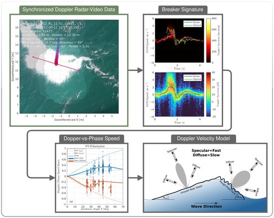
:Field-tower-based observations were used to estimate the Doppler velocity of deep water plunging breaking waves. About 1000 breaking wave events observed by a synchronized video camera and dual-polarization Doppler continuous-wave Ka-band radar at incidence angles varying from 25 to 55 degrees and various azimuths were analyzed using computer vision methods. Doppler velocities (DVs) associated with breaking waves were, for the first time, directly compared to whitecap optical velocities measured as the line-of-sight projection of the whitecap velocity vector (LOV). The DV and LOV were found correlated; however, the DV was systematically less than the LOV with the ratio dependent on the incidence angle and azimuth. The largest DVs observed at up-wave and down-wave directions were accompanied by an increase of the cross-section polarization ratio, HH/VV, up to 1, indicating a non-polarized backscattering mechanism. The observed DV was qualitatively reproduced in terms of a combination of fast specular (coherent) and slow non-specular (incoherent) returns from two planar sides of an asymmetric wedge-shaped breaker. The difference in roughness and tilt between breaker sides (the front face was rougher than the rear face) explained the observed DV asymmetry and was consistent with previously reported mean sea surface Doppler centroid data and normalized radar cross-section measurements.
1. Introduction
Studying the sea surface Doppler radar shifts has a long history, dating back to Crombie’s [1] discovery, which pioneered the high-frequency radar technology by using measured Doppler spectra as the basic input for sea surface current retrieval [2,3]. Because of the rapid growth in the number of new microwave satellite radar sensors over recent decades, the focus in shorter microwave bands has traditionally been on power (cross-section), rather than Doppler radar characteristics. However, understanding sea surface Doppler shift is instrumental in gaining a comprehensive understanding of the sea surface radar backscattering mechanisms [4,5,6,7,8,9,10,11,12].
Doppler scatterometry, aimed at the simultaneous wind and current retrievals at a high spatial resolution, has become more realistic as satellite radar technology has advanced [13,14,15,16,17]. Hence, explaining and understanding sea surface radar Doppler spectra are now not only a stand-alone academic task, but also a critical step in future mission data retrieval.
It is generally understood that the sea surface microwave Doppler shift contains the Bragg wave velocity modulated by longer surface wave orbital velocities [4,18,19]. This wave-induced Doppler velocity component is part of the total radar Doppler velocity, which also includes the desired component due to the footprint of mean sea surface currents. For practical oceanography retrieval needs, the two components should be separated.
Several complementary approaches have contributed to the understanding of the physics of sea surface radar echo. These include, but are not limited to asymptotic electromagnetic theories [20,21,22,23,24], empirical geophysical model function approaches [15,25,26], and/or semi-empirical modulation transfer function (MTF) concept models [27,28,29,30]. Using this latter method, a semi-empirical MTF-based Doppler centroid model, KaDOP, was developed [31] based on Ka-band Doppler radar measurements from a research tower in the Black Sea. The above models fairly well explain/predict the sea surface Doppler shifts. However, none of them directly involve one important phenomenon—wave breaking—which has a significant impact on sea surface radar backscattering [32,33,34,35,36].
A Doppler radar imaging model (DopRIM) [37,38] is a semi-empirical MTF-based model that takes wave breaking into account as a separate scattering mechanism. With the addition of wave breaking scattering, it was able to explain some Doppler shift features that were not explained by the theoretical MTF included in this model. Alternatively, asymptotic solutions can implicitly include wave breaking via sea surface non-Gaussianity [23,39,40], while the empirical MTF can also help explain the wave breaking contribution via cross-section modulations [31,41,42].
Because of the complexity of breaker Doppler shift representation, the direct inclusion of breakers into models is difficult. Breaking waves are usually associated with fast scatterers, which are thought to be responsible for the high-frequency tails of sea surface microwave Doppler spectra [43,44,45,46,47,48]. Using low-grazing-angle X-band radar observations of coastal surf, Farquharson et al. [49] demonstrated that the shallow water breaker Doppler velocity is dominated by the phase velocity of a breaking wave. Similarly, a significant increase in observed low-grazing-angle X-band Doppler velocity (up to the breaking wave phase velocity) has been reported [50,51] for waves entering the surf zone. Even for moderate incidence angles, the DopRIM [37,38] uses the same relationship between the breaker Doppler velocity and phase speed.
Yet, this intuitive relationship requires further confirmation. For example, Sletten et al. [11] demonstrated that, at low grazing angles, spilling breakers have Doppler speeds close to the wave crest speed, while for more intensive plunging breakers, the radar echo envelope propagates with a speed faster than the Doppler speed. In Ka-band laboratory experiments with steep gravity–capillary micro-scale wave breaking performed at moderate incidence angles, Ermakov et al. [36] reported a Doppler velocity close to the carrier wave phase speed for short >4 Hz waves and a difference between them for longer <3–3.5 Hz waves (with a slower Doppler velocity). Previously, Lee et al. [44] proposed a scenario in which fast (phase velocity) scatterers observed at the beginning of wave breaking were gradually replaced by slower (wave orbital velocity) scatterers as breakers age and decay.
All these findings imply that the breaker Doppler velocity is at least dependent on the scattering mechanism, which in turn is dependent on the breaking intensity, a specific stage of wave breaking, and the sensor look geometry (incidence angle and azimuth relative to the breaking wave crest, operating radar wavelength). The complex evolving breaker can be replaced by a simple time-independent model capable of describing observations at a specific configuration, depending on the dominant (in terms of cross-section) mechanism. Using the Black Sea tower Ka-band collocated radar–video measurements, it was investigated how the whitecap Doppler speed relates to its visual signature speed [52]. A manual examination of a few tens of whitecap events at moderate incidence angles [52] revealed that the Doppler speed is indeed slower than the breaker phase speed. This finding justified the omission of the explicit wave breaking contribution in the Doppler centroid KaDOP model [31] (remembering that breakers implicitly contribute to the empirical MTF) and was incorporated in a new DopRIM SAR [53,54].
Nonetheless, many details about the sea surface Doppler shifts caused by breakers remain unknown. This investigation started with a manual inspection of breaker Doppler properties [52]. Following that, a model for the breaker normalized radar cross-section (NRCS) was developed [55] using automated methods for breaker detection. In this paper, the same dataset was used to evaluate breaker Doppler shifts at various observation look geometries using computer vision breaker detection with far richer statistics than that for manual detection. Using these data, the observed Doppler velocity was, for the first time, directly compared to the visible (optical) line-of-sight velocity of whitecaps. Despite the fact that the two variables are connected, the Doppler velocity was systematically lower than the line-of-sight optical velocity. Their mean ratio depends on the incidence angle and azimuth look direction. A basic asymmetric wedge-shaped breaker model with a smooth transition between fast/specular (coherent) and slow/non-specular (non-coherent) scattering mechanisms, whose balance determines the resulting wave breaking Doppler signature, qualitatively explained this relationship.
The paper is organized as follows. Section 2 briefly describes the dataset used in the study. Section 3 presents the direct comparison between the optical and Doppler speeds of whitecaps. In Section 4, a simplified model of the breaker is developed to explain the observations. Section 5 summarizes the study and gives possible extensions of the presented framework.
2. Materials and Methods
The field data used in this study were collected between 2009 and 2015 from the Black Sea Research platform. This database includes Ka-band continuous-wave Doppler radar records accompanied by synchronous video records of the radar footprint. The data processing algorithm is described in detail in [31,52,56].
Briefly, the processing algorithm is focused on the detection of whitecap events within the radar footprint. The footprint is evaluated from the calibrated two-way radar pattern and known look geometry of the radar and video camera. The measurements were performed at 25, 30, 33, 35, 40, 45, 53, and 55 incidence angles, . Raw radar in-phase and quadrature signals, digitized by a 14-bit analog-to-digital (ADC) converter at 40 kHz, were averaged over 0.2 s time intervals, yielding instantaneous Doppler spectra, . Their zeroth and first moments were used to evaluate the instantaneous surface cross-section, , and Doppler frequency shift, , respectively:
where t is the time and f is the Doppler frequency.
The radar and video camera were synchronized by recording the same background noise audio signal from the camera’s microphone. These two identical signals recorded by the radar ADC and video camera were matched with accuracy better than one video frame (1/25 s) using the usual cross-correlation analysis.
In contrast to [31], the data collected at a large incidence angle, , were not considered here because, at such high incidence angles, the optical whitecap speed estimates are significantly distorted due to non-planar projection errors. For the duration of each detected whitecap event, the following radar and sea surface parameters were estimated and stored in the database: Doppler spectra, NRCS, instantaneous Doppler centroid velocity (DV), and whitecap geometrical parameters. The latter include whitecap area, length, speed, azimuth, and whitecap footprint fraction, Q:
where B is the binary image brightness ( for whitecaps, for a regular surface), G is the radar footprint on the mean sea horizontal plane, is the point coordinates on the mean sea surface, and R is the distance between the radar and -point. Every breaking event from the database was visualized (Figure 1) to gain deeper insights into the studied phenomenon, conduct a “quality control”, and discard possible fault detection cases. Examples of such a visualization can be found in the Supplementary Video S1.
In this study, the DV is the radial velocity (i.e., the component of velocity toward or away from the radar). It is defined as
where is the Doppler frequency shift and is the radar wavenumber. This radial direction is also termed the line-of-site (LOS) direction. The optical velocity (OV) was estimated from tracking a whitecap (using the radar–video processing illustrated in Figure 1) and reflects the phase velocity of a breaker, i.e., . For the majority of comparisons, the DV was compared to the LOS projection of the breaker optical velocity (LOV), i.e., , where is the breaker azimuth determined from the trajectory of the whitecap centroid.
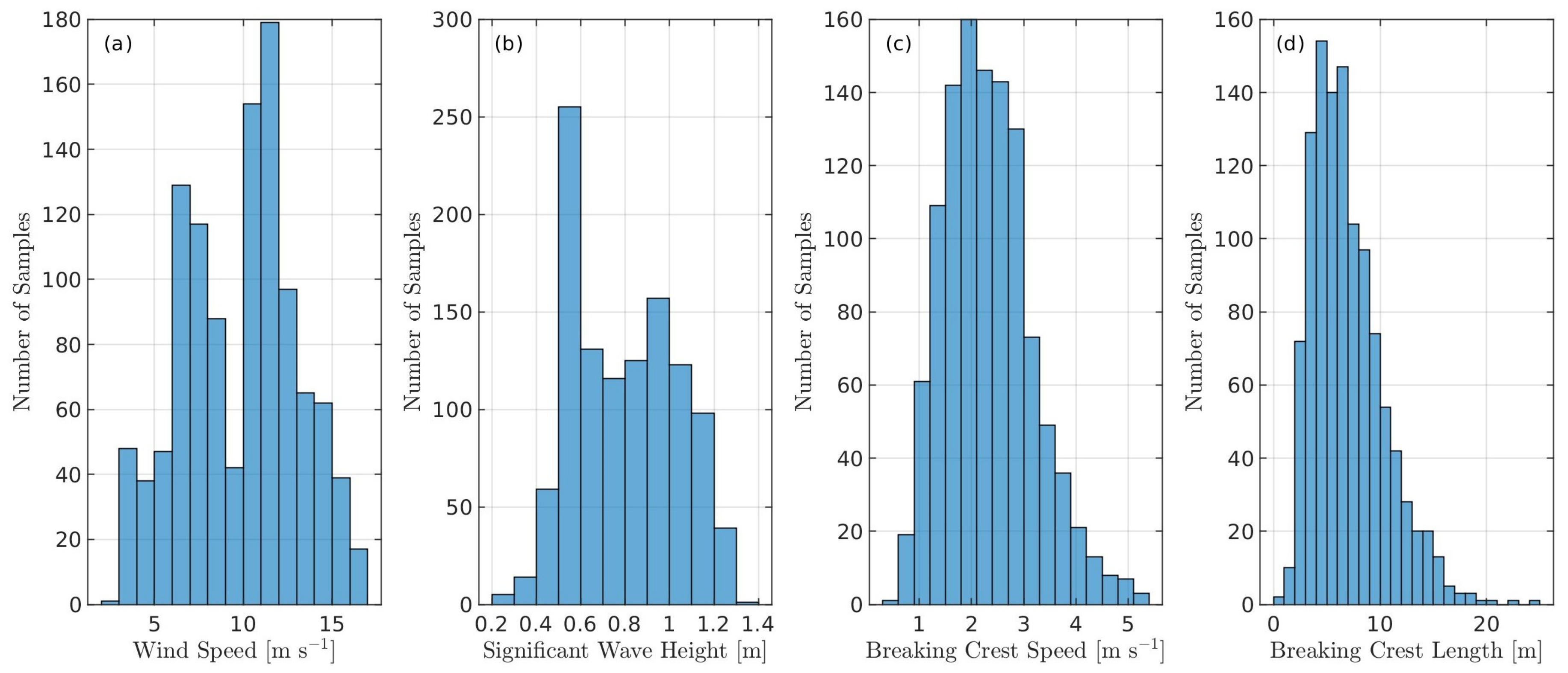
The measurements were collected in various environmental conditions, with the wind speed varying from 3 to 16 m s. However, the vast majority of breaking events were collected at 7–12 m s, with the significant wave height ranging from 0.5 to 1.1 m (Figure 2 and Table 1). Since only breaking wave cases were considered, any significant impact of the environmental conditions on the breaking wave structure was not expected and ignored in this study.
The median breaker speed in the dataset was ∼2.2 m s. Assuming that it corresponds to the phase speed of dominant breakers, this speed suggested breaking of ∼3.2 m-long waves. In turn, this corresponds to the breaking of ∼3.75 waves, where Hz is the typical wave spectrum peak frequency at the platform site. Shorter breakers were also present, but excluded from the consideration using the threshold. Such short breakers are too short to dominate the radar signal, given the background regular (non-breaking) surface scattering. The described processing technique retains only quite intense breaking events, and thus, only plunging breakers were considered in this study.
The total number of detected breaking events was 1100. It included about 140,000 processed frames (the video frame rate was 25 fps). For further analyses, two types of data were distinguished:
- “Instant” dataset: All processed frames were considered independently. One sample in the “instant” dataset was one video frame, with a radar footprint occupied by a breaker. Note that these data involved all breaking stages, including both young active whitecaps and decaying passive foam wakes following active breaker passage.
- “Average” dataset: All parameters corresponding to each breaking event, x, were weight-averaged using a time-varying Q, i.e., , with the overline denoting the time averaging over the whitecap lifetime. In this case, each sample corresponded to one breaking event, and the event mean whitecap and radar geometric characteristics were approximately related to the moment when the whitecap footprint fraction, Q, was maximized.
3. Results
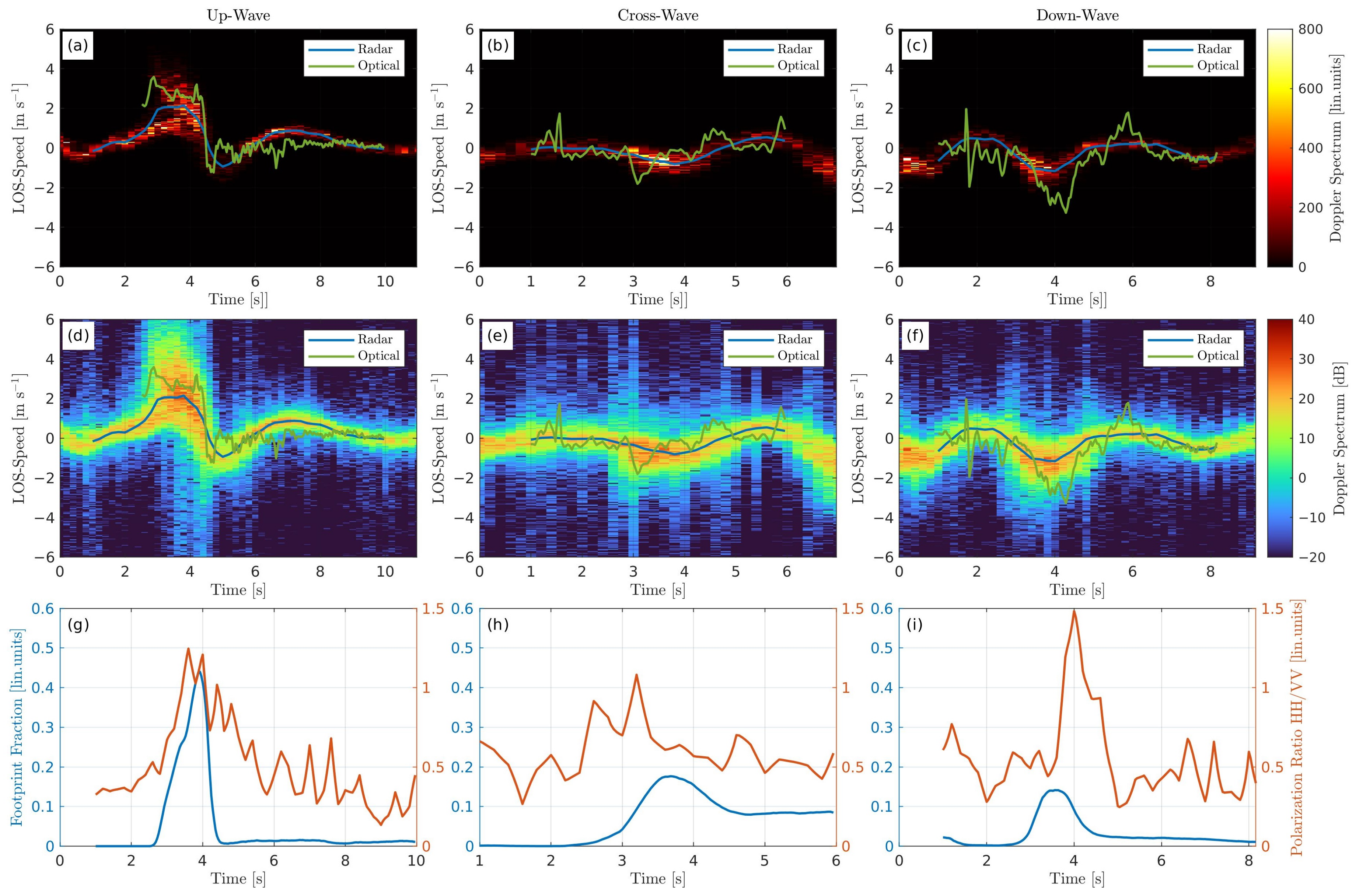
Three typical examples from the processed dataset are shown in Figure 3. They illustrate up-wave, cross-wave, and down-wave observations at (the up-wave case is the same as that shown in Figure 1).
The first prominent thing seen from the samples (Figure 3) was a Doppler spectrum widening during the peak of breaking events. This was especially the case for up-wave look direction. Both slow and fast populations of scatterers can be distinguished in this particular situation. The spectrum widening was better observed in the logarithmic scale (Figure 3d–f). Noticeably, the up-wave spectrum was wider than the down-wave and cross-wave ones.
Though the fast scatterers were seen by the radar, the instantaneous Doppler velocity (DV), estimated through the first moment of the Doppler spectrum (blue line in Figure 3a–f), was still dominated by slow motions. As a consequence, the line-of-sight optical velocity (LOV), i.e., an optical proxy for the DV, was always higher in magnitude than the DV, except for the cross-wave observation geometry, when both were near zero due to the vanishing LOS projection.
Noticeably, all three events were accompanied by similar increases in the polarization ratio between the HH and VV backscattering cross-section components (PR = ). Normally, the PR is less than 1 over a regular sea surface where the resonant (Bragg) backscattering mechanism dominates. During whitecap passage (Figure 3g–i), the observed PR values spiked up to 1 and even higher, reflecting a so-called non-polarized (NP) backscattering regime. Events with a PR higher than 1, which were also observed in the measurements, are known as super-events [57]. They are usually attributed to the Brewster damping of the VV signal and/or the effect of the multiple scattering typical for low-grazing-angle observations or steep surface features. In these measurements, similar super-events also can result from the speckle nature of the radar signal and the difference between the VV and HH footprints.
Although fast scatterers were practically visible only in up-wave data, the non-polarized backscattering (corresponding to the PR spikes) was observed in all three cases. This means that both fast and slow scatterers belong to the NP category. It is also interesting that, for the up-wave direction, the whitecap (Q) and PR spikes were almost coincident in time. For the cross-wave direction, the Q spike lagged the PR spike. For the down-wave direction, the PR spike lagged the Q spike. This suggested that, depending on the look geometry, different whitecap parts dominated the NP backscattering.
In this study, we attempted to estimate how fast the DV was in comparison with the breaking wave phase velocity (estimated from the optical whitecap detection). The relationship between the Doppler and optical velocities can vary widely, as the examples in Figure 3 illustrate. However, regardless of the rather strong scatter between the DV and LOV, some average relationship between them can be deduced.
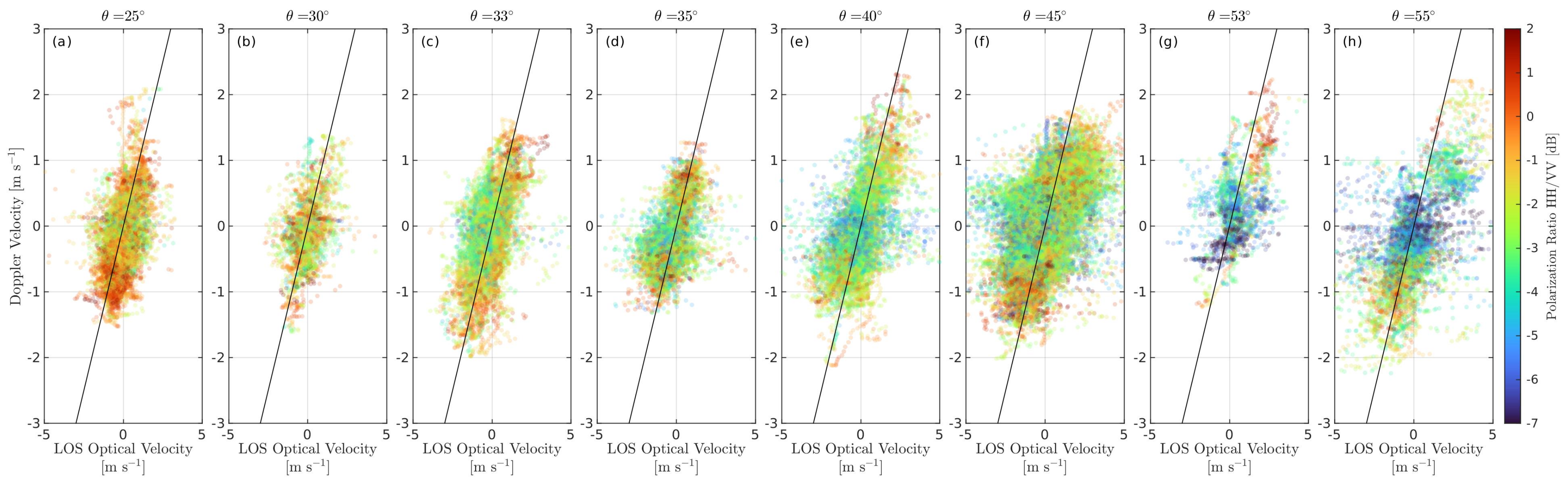
Figure 4 shows the DV versus LOV scatterplots for each incidence angle based on the “instant” dataset (see the dataset definition above). The data points group around the lines, but the scatter is huge since the “instant” dataset includes all stages of breaker evolution, e.g., the LOV may correspond to the remaining foam wake, which does not impact the DV.
Independent of the incidence angle, the common feature of all panels in Figure 4 is that the PR was maximized at both edges of the point clouds. These high positive and negative DV values correspond to up-wave (positive) and down-wave (negative) radar observations. This indicates the presence of the NP in both the up-wave and down-wave cases. In the cross-wave direction (DV ≈ 0), the PR decreased, suggesting a weaker NP contribution. The general tendency reflecting PR values closer to 1 for smaller (where specular reflections dominate) held. Yet, even at moderate incidence angles, , the PR was still about 1 for the highest velocity magnitudes.
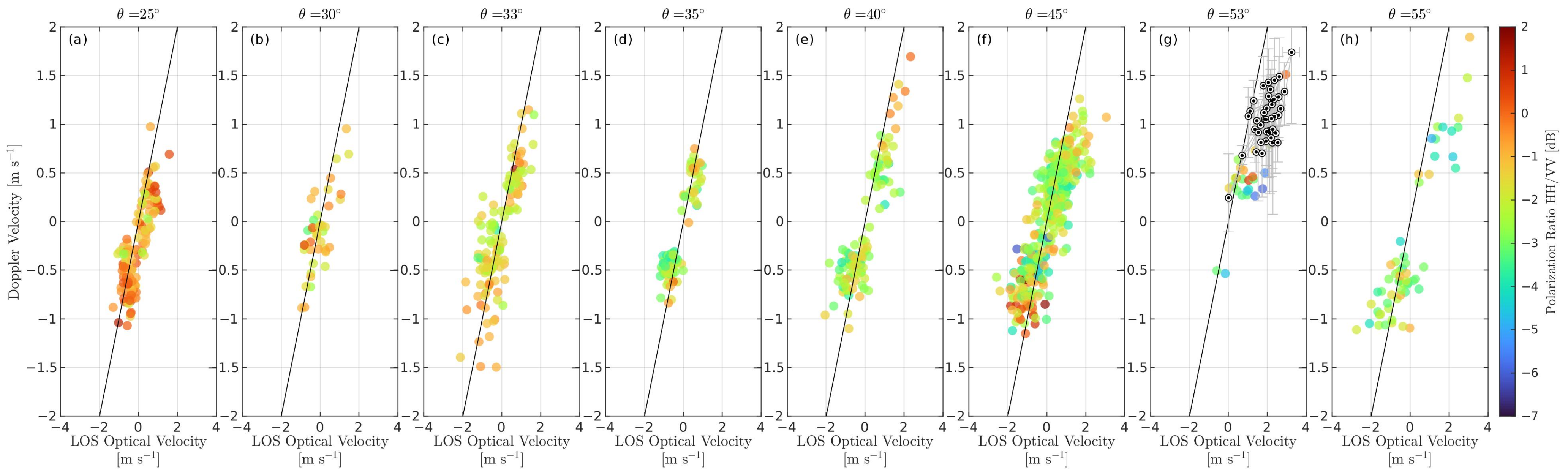
Less noisy pictures can be achieved using the “average” dataset (Figure 5). Now, each point corresponds to a particular breaking event, focusing on conditions during maximum Q within the radar footprint. For this “average” dataset, the number of points was significantly less, but the noise scatter dropped as well. At large incidence angles, , a tendency of DV “saturation”, |DV| < |LOV|, was observed. This agreed with our manually derived estimates [52], also shown in Figure 5g.
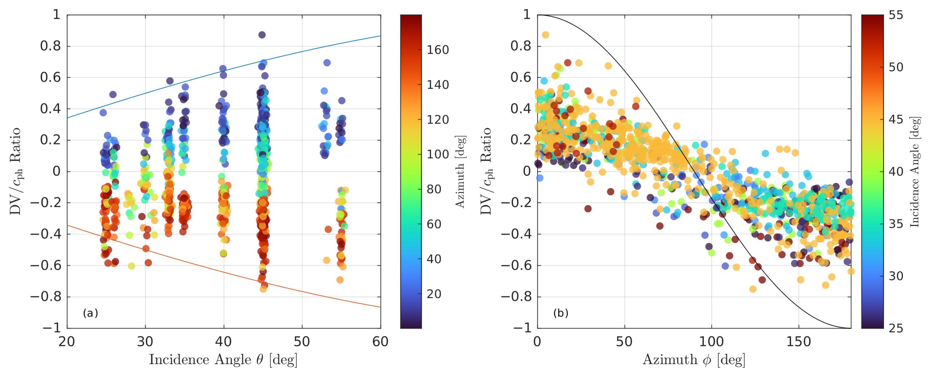
Next, the observed DV was normalized by the breaker phase velocity, , derived from the optical velocity magnitude (Figure 6). This normalized showed that the DV was always less than the phase velocity, except for several presumably erroneous points where the optical velocity was possibly underestimated. In general, the data fell within the limiting corridor fairly well, while the azimuth distribution was cosine-like, , but scaled by the mean factor.
One may note that Figure 5 reveals multiple |DV| ≥ |LOV| cases, while they are not that apparent in Figure 6. Figure 6a shows the expected corridor for the values at a given incidence angle, . This representation emphasizes only the fastest DV data (up-wave or down-wave) that fell out of the corridor width. In contrast, Figure 5 compares the DV data with the LOV data. This means that the majority of the |DV| ≥ |LOV| cases in Figure 5 came from near-cross-wave directions.
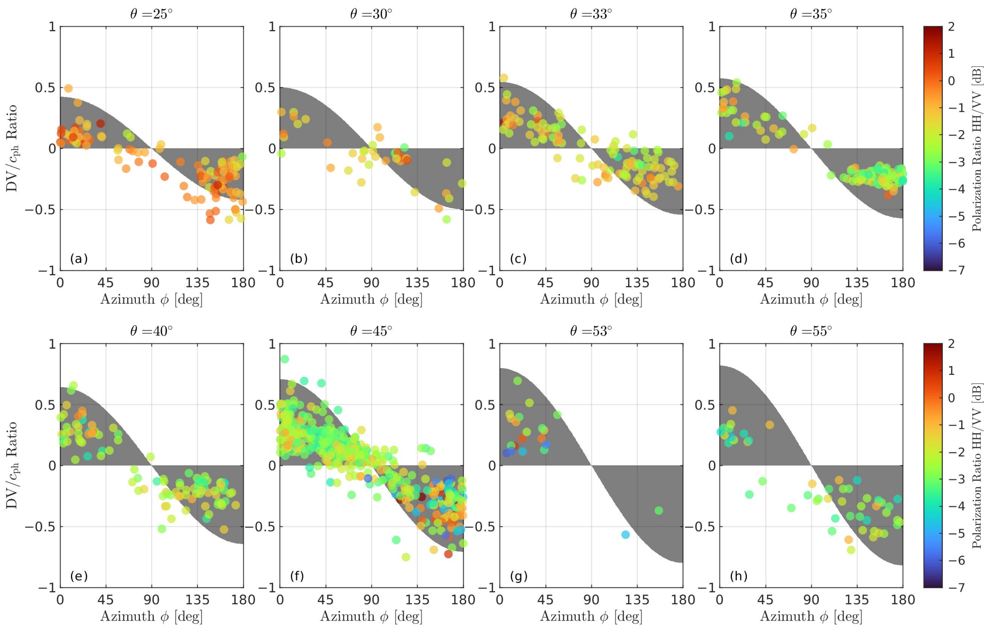
This is better visualized in Figure 7, which shows the same normalized DV as in Figure 6, , as a function of the breaker azimuth for each incidence angle group. This figure confirmed that the cases corresponded mostly to near-zero LOS projection, , while close to the up-/down-wave directions, the magnitude of the DV was usually less than . A statistical explanation for that may involve the presence of random errors inherent to both the DV and measurements, which became relatively more important when the mean values vanished. For the DV, it may also be related to the orbital motions within the footprint that were not related to the observed whitecap. Their effect on the DV was presumably weak because a whitecap is a much “brighter” object in the NRCS. However, errors introduced by regular surface velocities may increase at small incidence angles, where the background may not be that weak in comparison with the breaker NRCS (Figure 7a).
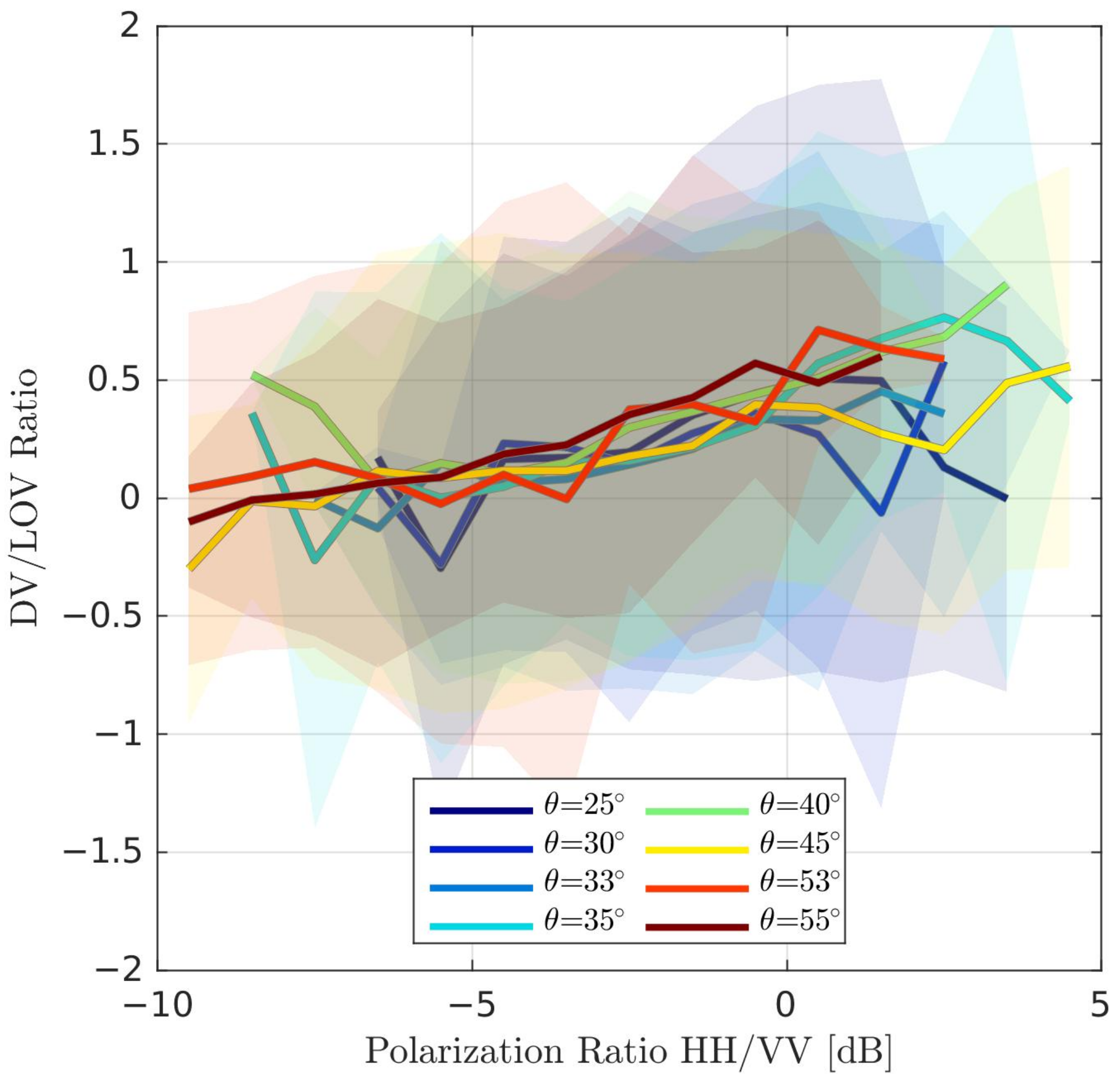
An important feature revealed by the observations is that the PR was maximized for large speeds and mostly in the up-wave and down-wave directions. This is better seen for the “instant” (Figure 4) than for the “average” (Figure 5 and Figure 7) dataset because the PR peak was not necessarily coincident with the Q peak (Figure 3). To gain deeper insights into the connections between the breaker PR and DV, only near up-wave and down-wave samples ( and ) were selected from the “instant” dataset and plotted as the normalized DV/LOV versus the PR (Figure 8). Noticeably, the bin-averaged normalized DV systematically increased with the PR at all incidence angles. This means the stronger the NP return is, the closer the DV to the breaking wave phase velocity is. Yet, the bin-averaged DV never reached the phase velocity, with maximum values of ∼0.5–0.7, again indicating that the “pure” NP return events (with the PR approaching 1) did not always propagate as fast as the breaking wave phase velocity (as demonstrated in Figure 3).
4. Discussion
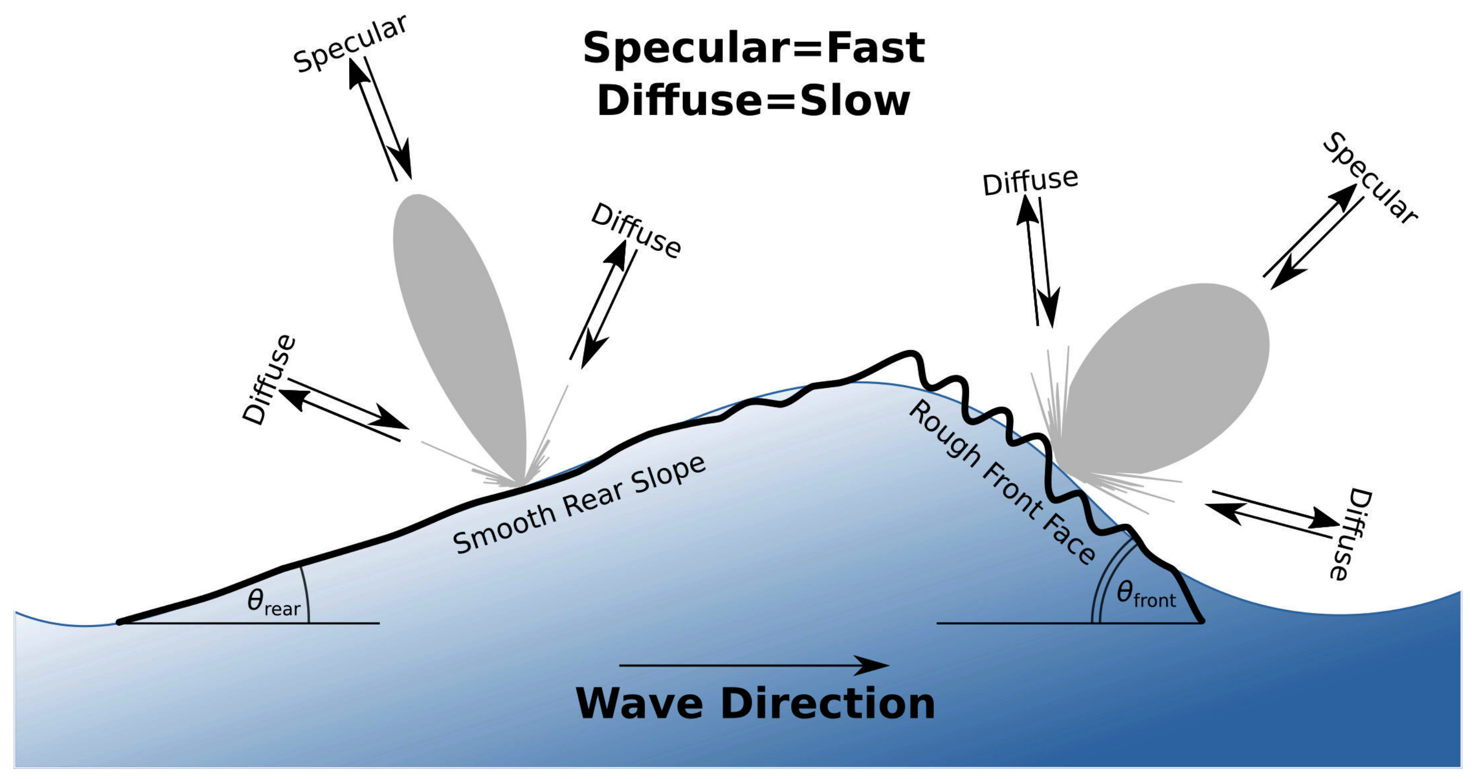
The main result presented in this study suggested that the observed DV of breaking wave tended to its phase velocity, but never reached it. The DV was higher when the PR was closer to 1 (when the scattering was close to the NP regime). However, even in this case, the DV was only a fraction of . This can be explained by a combination of specular (presumably fast) and diffuse (slow) backscattering mechanisms during breaking events. Visual observations of breakers, as well as their numerical simulations, e.g., [58], suggested that the roughness generated by the active breaking crest is further “embedded” into the water and, thus, propagates with the wave orbital velocity, while the breaking crest itself propagates faster, with the characteristic velocity closer to the carrier wave phase velocity. This is the obvious reason why breaking waves have rough tails.
If rough patches scatter e.m. radiation coherently, the scattering mechanism is specular-like and the whole glinting facet plays the role of a coherent scatterer. Then, the associated DV is the velocity of this facet, which is close to the carrying wave phase velocity:
Otherwise, when the radar backscattering is incoherent, the surface is disintegrated into numerous independent (incoherent) scatterers. Their velocities approach liquid particle velocities, and the DV, thus, drops to the orbital wave velocity. A particular case of such incoherent mechanisms is the resonant (Bragg-like) scattering in which scatterers have their inherent velocity determined by the phase velocity of the resonant (Bragg) wave component, . Note both approaching and moving away waves resonate; thus, the total Bragg velocity is determined by the balance between their amplitudes. For regular, non-breaking sea surfaces, one of these wave components normally dominates. However, this is not the case in strongly rough breaking patches, which presumably have a quasi-isotropic roughness spectrum. Thus, no matter what solution is better for the incoherent backscattering component—e.g., the small-perturbation method (SPM) or Kirchhoff approximation (KA) [18,59,60]—its velocity will tend to be close to the orbital wave velocity [21].
To further demonstrate the plausibility of this concept, Figure 9 shows the DV normalized by the breaking wave phase velocity azimuth projection, , but only in up-wave and down-wave 45-azimuth intervals (as in Figure 8). Now, the up-wave and down-wave DVs have opposite signs due to the absolute value of . Again, note that all observed DV values were below their corresponding breaker phase velocities, , and the majority of normalized DV values fell into the limiting corridor.
The lower range of data scatter in Figure 9 was not zero for either up-wave or down-wave data and was roughly determined by the average steepness of breaking waves, , which defines the magnitude of the wave orbital velocity. The typical measured values of differ from the classical theoretical 0.4 Stokes steepness [61]. For example, Scott et al. [62] reported a 0.12 median breaker steepness from open ocean measurements, while Toffoli et al. [63] found to be about 0.55/0.44 for the front/rear slope of the waves based on laboratory and field data. Without dwelling on the details, the average breaker steepness was set, , to fit the measurements shown in Figure 9.
Note that, in the case of incoherent (slow) scattering, the scattering centers were distributed over the breaking wave profile and, thus, had the LOS projection velocity and NRCS distribution, which both varied along the breaker profile. A convolution of these two parameters determined the total DV associated with a breaking wave, by analogy with MTF concept averaging. For the sake of simplicity, an intuitive expectation that the strongest backscattering source is localized at some particular position on the carrier wave was adopted. Then, the slow velocity can be roughly represented as
where is the wave phase at which the scatterer roughness is concentrated. As a first guess, the roughness concentration was collocated with the wave crest, .
The partitioning between fast and slow regimes differed for the up-wave and down-wave directions (Figure 9, blue and reddish colors). For the up-wave observation conditions, the normalized DV was maximized at ∼37. For the down-wave observation conditions, there was a peak in magnitude at lower incidence angles, ∼30, and an increase at large ones, . In this speculative model, the actual DV is then a combination of the fast and slow velocities:
where W is the measure of the coherency (“specularity”) of the backscattering mechanism: for pure coherent (specular) scattering; for pure incoherent (diffusive) scattering.
To estimate W, the previous NRCS study [31] was followed, and the only, to the best of our knowledge, direct measurement of breaker roughness [64] was utilized. In [64], it was found, however, that the coherent backscattering part vanishes for artificial stationary breakers generated by a submerged hydrofoil in a liquid flow. Their incoherent breaker cross-section was adequately modeled by the KA near the breaker crest and by the SPM over the breaker tail. Their analysis, however, somewhat contradicts our and other measurements because the solely incoherent scattering is inconsistent with the presence of fast scatterers. Thus, a coherent part was considered, e.g., using the high-frequency KA limit or geometric optics (GO) approach with a corrected reflection coefficient:
where is the local incidence angle, is the mean-squared slope (MSS) of the scattering surface in the wavenumber range, and is the effective reflection coefficient, which is the Fresnel reflection coefficient, at normal incidence attenuated by a factor due to small-scale roughness, and , where is the small-scale surface elevation variance (for the Ka band, ).
The incoherent breaker backscattering was estimated directly from the data of [64] as dB. Then, the weight factor W in Equation (7) reads
To highlight the difference between the up-wave and down-wave cases, the following simplified breaker observation geometry was considered (Figure 10).
In this speculative model, the breaker has two plane faces scattering independently in the up-wave (front face only) and down-wave (rear face only) directions. The local incidence angle, , in Equation (8) is replaced by , where is either the front or rear face slope. This approximation may fail at near-nadir geometry, where both faces may contribute, but the present measurements spanned only moderate incidence angles, . Equations (5)–(9) determine the transition between slow and fast regimes along the breaker profile. Three parameters, , , and , determine the speculative breaker model’s behavior. These parameters were tuned to fit the model to the observations (Table 2).
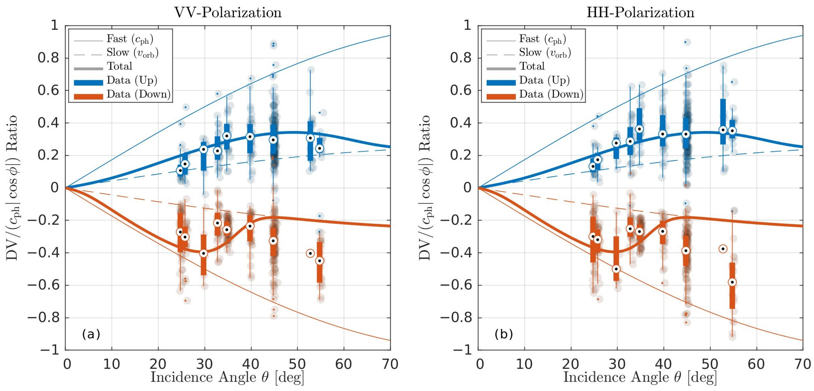
For up-wave observations, the proposed model qualitatively explained the presence of a wide “bump” in the normalized DV dependence on the incidence angle that is centered at . For down-wave observations, it suggested the presence of a “bump” in the normalized DV at smaller incidence angles, (Figure 9). The asymmetry between the front and rear breaking wave faces (the front is steeper) is necessary to explain the observations, and it agreed well with well-known skewed profiles of breaking waves, e.g., [63,65,66,67,68]. For down-wave observations, smooth (smaller MSS and small-scale variance) rear faces produced strong, and thus fast, reflections, which explained the previously observed unusual “down-wave > up-wave” NRCS [69] and Doppler centroid [31] data in the Ka band at small , as well as independent Ku/Ka precipitation radar measurements [70,71].
Yet, for the down-wave direction, the increase of the DV magnitude at large was not explained by this simple two-face speculative model (Figure 9). As seen from Figure 5, the PR for this observation geometry was still large, indicating the NP nature of the backscattering mechanism. Conceptually, an additional specular facet can be added as a rear slope feature to explain these observations. The “bump” in down-wave normalized DV data at high-incidence angles, however, looks quite wide, suggesting that this additional specular facet had a large MSS or this facet was a cylindrical roller feature. Thus, it is argued that different look geometries may involve different mean breaker profiles because the radar backscattering at different look geometries is dominated by different breaking types (stages).
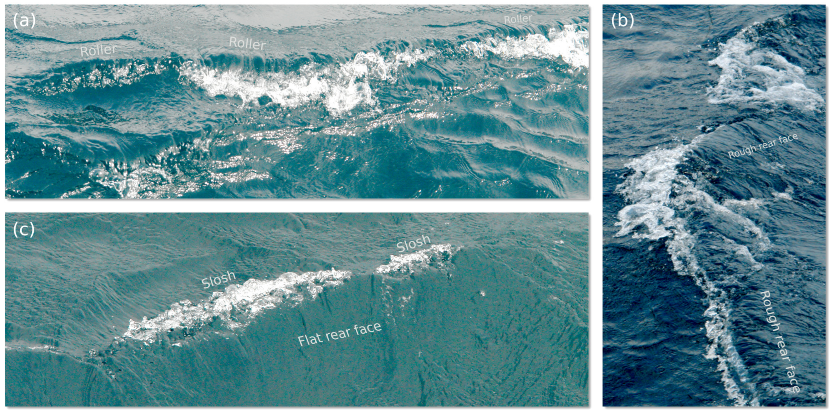
As shown in Figure 3a,c, the PR peak for the up-wave and down-wave directions developed at different times relative to the whitecap (Q) peak. For the down-wave look geometry, the PR peak occurred after the Q peak. Thus, at high incidence angles, when specular reflection from the smooth rear slope is no longer important, one may expect a contribution from, e.g., a cylindrical roller at the breaking wave crest. Figure 11 demonstrates a variety of possible plunging breaking wave geometries. These photos were taken at an incidence angle of about 50 with a zoomed 10-wide field-of-view. Thus, the features displayed by these photos were also “seen” by radar at . Such breaking sea surface features (Figure 11) have also been used to explain low-grazing-angle radar observations, a so-called “slosh” feature [34,72]. In the breaker NRCS model [55], a similar feature was also necessary to better explain the down-wave observations. Further modeling is required for a more accurate representation of the breaking wave geometry.
Finally, the present analysis complements the study by Ericson et al. [64], who suggested ignoring the specular reflection for observations based on their breaking roughness measurements and e.m. modeling. Ericson et al. [64] found that the exponent in the effective Fresnel coefficient is about (see their Figure 8 and Figure 10 for the crest wave position). Hence, is quite small, which allowed them to ignore the coherent (specular) contribution. In our case, this parameter had the same order of magnitude, , for the up-wave look geometry. Although this value is only ∼3% of the regular Fresnel coefficient, even that magnitude was enough to explain the fast contribution to the observed breaking wave DV.
5. Conclusions
This paper continues the previous analysis [55] of joint synchronous collocated radar and video observations of deep water breaking waves collected from the Black Sea research platform. After analyzing the whitecap normalized radar cross-section in [55], here, the focus was on the investigation of the Doppler shifts associated with whitecap passages through the radar footprint. Simultaneous radar and video measurements were carried out in different experiments during 2009–2015. They covered a wide range of incidence angles between 25 and 55 and various azimuth look directions relative to the breaking wave trajectories (from up-wave to down-wave). The environmental conditions also varied with a 7–12 m wind speed and a 0.5–1.1 m significant wave height. However, their possible impacts were ignored because only breaker occurrences were analyzed. The total number of analyzed events was about 1100. Since only whitecap events that are relatively large compared to the typical 3 m by 5 m radar footprint could be detected by video processing, the analyzed events mostly represented intense plunging breakers.
The basic idea of the study was to estimate the radar Doppler velocity (DV) of individual breakers and compare it to the breaker optical velocity (OV), which, by definition, is the phase velocity of a breaking wave. The DV was found to generally be correlated with the OV. Although the scatter between the instantaneous DV and line-of-sight (LOS) OV projection (LOV) was quite strong, the general behavior was DV ≈ LOV for small speeds (mostly cross-wave cases) and |DV| < |LOV| for large speeds (mostly the up-wave or down-wave cases). The polarization ratio during breaking events was maximized in the up-wave and down-wave look directions, indicating the domination of the non-polarized (NP) scattering mechanism. For these two look directions, the DV scaled by the LOV tended to increase with the increasing PR for all (25–55) incidence angles. Yet, the average DV/LOV ratio did not increase to 1, even at the maximal PR values, PR ≥ 1, remaining at about DV/LOV = 0.5–0.7.
This suggested that the breaking wave DV is a combination of fast and slow scatterers, where fast scatterers are specular (coherent) reflections from glinting facets moving with the phase velocity of a breaker and slow scatterers are (non-coherent) diffuse reflections from the breaker roughness moving the orbital velocity of a breaking wave. To explain the observed DV/LOV ratio, a speculative model of a wedge-shaped breaker with a planar front and rear faces was adopted. The DV of each face (front for the up-wave look direction and rear for the down-wave look direction) was determined by the weighted average of the phase and orbital wave velocity, where the weight was determined by the relative contribution of the specular (coherent) and diffusive (non-coherent) scattering components. The model, fit to the observations by varying the mean front/rear face slope, mean-squared slope, and small-scale variance, suggested an asymmetric breaker shape with the front face being steeper and rougher than the rear face.
This simplified model agreed with the NRCS analysis of the same dataset [55] and can help to explain the previously observed unusual “upwind < downwind” asymmetry in the Ka-band Doppler centroid [31] and NRCS [69]. Our further efforts will focus on a self-consistent fusion of the NRCS and Doppler breaker models, which should be included in the advanced radar imaging model.
Supplementary Materials
The following supporting information can be downloaded at: https://doi.org/10.5281/zenodo.7780687, Video S1: Examples of joint radar–video processing.
Author Contributions
Conceptualization, V.N.K. and Y.Y.Y.; methodology, Y.Y.Y.; software, Y.Y.Y.; validation, S.A.G., B.C. and V.N.K.; formal analysis, Y.Y.Y.; investigation, V.N.K. and Y.Y.Y.; resources, Y.Y.Y.; data curation, Y.Y.Y.; writing—original draft preparation, Y.Y.Y.; writing—review and editing, S.A.G. and B.C.; visualization, Y.Y.Y.; supervision, V.N.K. and Y.Y.Y.; funding acquisition, V.N.K. All authors have read and agreed to the published version of the manuscript.
Funding
The data analysis and radar modeling performed in this work were supported by the Russian Science Foundation under Grant 21-47-00038 (https://rscf.ru/en/project/21-47-00038/, accessed on 25 February 2023). The field experiments were sponsored by the MHI RAS State Order (Goszadanie) FNNN-2021-0004. The sea surface modeling approach was developed within the frame of the RSHU State Order (Goszadanie) 0763-2020-0005. S.A.G. was supported by the NASA Physical Oceanography.
Data Availability Statement
Not applicable.
Conflicts of Interest
The authors declare no conflict of interest.
Abbreviations
The following abbreviations are used in this manuscript:
| DV | Doppler velocity |
| LOS | Line-of-sight |
| LOV | Line-of-sight optical velocity |
| MSS | Mean-squared slope |
| MTF | Modulation transfer function |
| NP | Non-polarized |
| NRCS | Normalized radar cross-section |
| OV | Optical velocity |
| PR | Polarization ratio |
References
- Crombie, D.D. Doppler spectrum of sea echo at 13.56 mc/s. Nature 1955, 175, 681–682. [Google Scholar] [CrossRef]
- Hasselmann, K. Determination of ocean-wave spectra from Doppler radio return from the sea surface. Nat. Phys. Sci. 1971, 229, 16–17. [Google Scholar] [CrossRef]
- Barrick, D.E. HF radio oceanography—A review. Bound.-Layer Meteorol. 1978, 13, 23–43. [Google Scholar] [CrossRef]
- Pidgeon, V.W. Doppler dependence of radar sea return. J. Geophys. Res. 1968, 73, 1333–1341. [Google Scholar] [CrossRef]
- Long, M. On a two-scatterer theory of sea echo. IEEE Trans. Antennas Propag. 1974, 22, 667–672. [Google Scholar] [CrossRef]
- Jessup, A.T.; Keller, W.C.; Melville, W.K. Measurements of sea spikes in microwave backscatter at moderate incidence. J. Geophys. Res. Oceans 1990, 95, 9679–9688. [Google Scholar] [CrossRef]
- Plant, W.J.; Keller, W.C. Evidence of bragg scattering in microwave doppler spectra of sea return. J. Geophys. Res. Oceans 1990, 95, 16299–16310. [Google Scholar] [CrossRef]
- Lee, P.H.Y.; Barter, J.D.; Beach, K.L.; Caponi, E.; Hindman, C.L.; Lake, B.L.; Rungaldier, H.; Shelton, J.C. Power spectral lineshapes of microwave radiation backscattered from sea surfaces at small grazing angles. IEE Proc.-Radar Sonar Navig. 1995, 142, 252–258. [Google Scholar] [CrossRef]
- Walker, D. Experimentally motivated model for low grazing angle radar Doppler spectra of the sea surface. IEE Pro-Radar Sonar Navig. 2000, 147, 114–120. [Google Scholar] [CrossRef]
- Dano, E.B.; Lyzenga, D.R.; Perlin, M. Radar backscattering from mechanically generated transient breaking waves–Part 1: Angle of incidence dependence and high resolution surface morphology. IEEE J. Ocean. Eng. 2001, 26, 181–200. [Google Scholar] [CrossRef]
- Sletten, M.A.; West, J.C.; Liu, X.; Duncan, J.H. Radar investigations of breaking water waves at low grazing angles with simultaneous high-speed optical imagery. Radio Sci. 2003, 38, 1110. [Google Scholar] [CrossRef]
- Plant, W.J. Whitecaps in deep water. Geophys. Res. Lett. 2012, 39, L16601. [Google Scholar] [CrossRef]
- Chapron, B.; Collard, F.; Ardhuin, F. Direct measurements of ocean surface velocity from space: Interpretation and validation. J. Geophys. Res. Oceans 2005, 110, C07008. [Google Scholar] [CrossRef]
- Bao, Q.; Dong, X.; Zhu, D.; Lang, S.; Xu, X. The feasibility of ocean surface current measurement using pencil-beam rotating scatterometer. IEEE J. Sel. Top. Appl. Earth Obs. Remote Sens. 2015, 8, 3441–3451. [Google Scholar] [CrossRef]
- Rodriguez, E.; Wineteer, A.; Perkovic-Martin, D.; Gál, T.; Stiles, B.; Niamsuwan, N.; Rodriguez Monje, R. Estimating ocean vector winds and currents using a Ka-Band pencil-beam Doppler scatterometer. Remote Sens. 2018, 10, 576. [Google Scholar] [CrossRef] [Green Version]
- Ardhuin, F.; Brandt, P.; Gaultier, L.; Donlon, C.; Battaglia, A.; Boy, F.; Casal, T.; Chapron, B.; Collard, F.; Cravatte, S.; et al. SKIM, a candidate satellite mission exploring global ocean currents and waves. Front. Mar. Sci. 2019, 6, 209. [Google Scholar] [CrossRef] [Green Version]
- Gommenginger, C.; Chapron, B.; Hogg, A.; Buckingham, C.; Fox-Kemper, B.; Eriksson, L.; Soulat, F.; Ubelmann, C.; Ocampo-Torres, F.; Nardelli, B.B.; et al. SEASTAR: A Mission to Study Ocean Submesoscale Dynamics and Small-Scale Atmosphere-Ocean Processes in Coastal, Shelf and Polar Seas. Front. Mar. Sci. 2019, 6, 457. [Google Scholar] [CrossRef] [Green Version]
- Valenzuela, G.R. Theories for the interaction of electromagnetic and ocean waves—A review. Bound.-Layer Meteorol. 1978, 13, 61–85. [Google Scholar] [CrossRef]
- Kanevsky, M.B. Radar Imaging of the Ocean Waves; Elsevier: Amsterdam, The Netherlands, 2009. [Google Scholar] [CrossRef]
- Voronovich, A.G.; Zavorotny, V.U. Theoretical model for scattering of radar signals in Ku- and C-bands from a rough sea surface with breaking waves. Waves Random Media 2001, 11, 247–269. [Google Scholar] [CrossRef]
- Mouche, A.A.; Chapron, B.; Reul, N.; Collard, F. Predicted Doppler shifts induced by ocean surface wave displacements using asymptotic electromagnetic wave scattering theories. Waves Random Media 2008, 18, 185–196. [Google Scholar] [CrossRef]
- Nouguier, F.; Guerin, C.; Soriano, G. Analytical techniques for the doppler signature of sea surfaces in the microwave Regime—I: Linear surfaces. IEEE Trans. Geosci. Remote Sens. 2011, 49, 4856–4864. [Google Scholar] [CrossRef] [Green Version]
- Nouguier, F.; Guerin, C.; Soriano, G. Analytical techniques for the doppler signature of sea surfaces in the microwave Regime—II: Nonlinear surfaces. IEEE Trans. Geosci. Remote Sens. 2011, 49, 4920–4927. [Google Scholar] [CrossRef] [Green Version]
- Karaev, V.; Titchenko, Y.; Panfilova, M.; Meshkov, E. The Doppler Spectrum of the Microwave Radar Signal Backscattered from the Sea Surface in Terms of the Modified Bragg Scattering Model. IEEE Trans. Geosci. Remote Sens. 2020, 58, 193–202. [Google Scholar] [CrossRef]
- Mouche, A.A.; Collard, F.; Chapron, B.; Dagestad, K.F.; Guitton, G.; Johannessen, J.A.; Kerbaol, V.; Hansen, M.W. On the use of doppler shift for sea surface wind retrieval from SAR. IEEE Trans. Geosci. Remote Sens. 2012, 50, 2901–2909. [Google Scholar] [CrossRef]
- Martin, A.C.H.; Gommenginger, C.P.; Quilfen, Y. Simultaneous ocean surface current and wind vectors retrieval with squinted SAR interferometry: Geophysical inversion and performance assessment. Remote Sens. Environ. 2018, 216, 798–808. [Google Scholar] [CrossRef] [Green Version]
- Romeiser, R.; Thompson, D.R. Numerical study on the along-track interferometric radar imaging mechanism of oceanic surface currents. IEEE Trans. Geosci. Remote Sens. 2000, 38, 446–458. [Google Scholar] [CrossRef] [Green Version]
- Elyouncha, A.; Eriksson, L.E.B.; Romeiser, R.; Ulander, L.M.H. Measurements of sea surface currents in the Baltic Sea region using spaceborne along-track InSAR. IEEE Trans. Geosci. Remote Sens. 2019, 57, 8584–8599. [Google Scholar] [CrossRef]
- Moiseev, A.; Johnsen, H.; Johannessen, J.A.; Collard, F.; Guitton, G. On removal of sea state contribution to Sentinel-1 Doppler shift for retrieving reliable ocean surface current. J. Geophys. Res. Ocean. 2020, 125, e2020JC016288. [Google Scholar] [CrossRef]
- Elyouncha, A.; Eriksson, L.E.B.; Romeiser, R.; Ulander, L.M.H. Empirical Relationship Between the Doppler Centroid Derived from X-Band Spaceborne InSAR Data and Wind Vectors. IEEE Trans. Geosci. Remote Sens. 2022, 60, 4201120. [Google Scholar] [CrossRef]
- Yurovsky, Y.Y.; Kudryavtsev, V.N.; Grodsky, S.A.; Chapron, B. Sea surface Ka-band Doppler measurements: Analysis and model development. Remote Sens. 2019, 11, 839. [Google Scholar] [CrossRef]
- Kalmykov, A.I.; Pustovoytenko, V.V. On polarization features of radio signals scattered from the sea surface at small grazing angles. J. Geophys. Res. 1976, 81, 1960–1964. [Google Scholar] [CrossRef]
- Phillips, O.M. Radar returns from the sea surface–Bragg scattering and breaking waves. J. Phys. Oceanogr. 1988, 18, 1063–1074. [Google Scholar] [CrossRef]
- Kudryavtsev, V.; Hauser, D.; Caudal, G.; Chapron, B. A semiempirical model of the normalized radar cross-section of the sea surface 1. Background model. J. Geophys. Res. Oceans 2003, 108, C08054. [Google Scholar] [CrossRef] [Green Version]
- Sergievskaya, I.A.; Ermakov, S.A.; Ermoshkin, A.V.; Kapustin, I.A.; Shomina, O.V.; Kupaev, A.V. The Role of Micro Breaking of Small-Scale Wind Waves in Radar Backscattering from Sea Surface. Remote Sens. 2020, 12, 4159. [Google Scholar] [CrossRef]
- Ermakov, S.A.; Sergievskaya, I.A.; Dobrokhotov, V.A.; Lazareva, T.N. Wave Tank Study of Steep Gravity-Capillary Waves and Their Role in Ka-Band Radar Backscatter. IEEE Trans. Geosci. Remote Sens. 2022, 60, 4202812. [Google Scholar] [CrossRef]
- Johannessen, J.A.; Chapron, B.; Collard, F.; Kudryavtsev, V.; Mouche, A.; Akimov, D.; Dagestad, K.F. Direct ocean surface velocity measurements from space: Improved quantitative interpretation of Envisat ASAR observations. Geophys. Res. Lett. 2008, 35, 22608. [Google Scholar] [CrossRef] [Green Version]
- Hansen, M.W.; Kudryavtsev, V.; Chapron, B.; Johannessen, J.A.; Collard, F.; Dagestad, K.F.; Mouche, A.A. Simulation of radar backscatter and Doppler shifts of wave-current interaction in the presence of strong tidal current. Remote Sens. Environ. 2012, 120, 113–122. [Google Scholar] [CrossRef] [Green Version]
- Mouche, A.A.; Chapron, B.; Reul, N.; Hauser, D.; Quilfen, Y. Importance of the sea surface curvature to interpret the normalized radar cross section. J. Geophys. Res. Oceans 2007, 112, C10002. [Google Scholar] [CrossRef] [Green Version]
- Su, X.; Zhang, X.; Dang, H.; Tan, X. Analysis of microwave backscattering from nonlinear sea surface with currents: Doppler spectrum and SAR images. Int. J. Microw. Wirel. Technol. 2020, 12, 598–608. [Google Scholar] [CrossRef]
- Yurovsky, Y.Y.; Kudryavtsev, V.N.; Chapron, B.; Grodsky, S.A. Modulation of Ka-band Doppler radar signals backscattered from the sea surface. IEEE Trans. Geosci. Remote Sens. 2018, 56, 2931–2948. [Google Scholar] [CrossRef] [Green Version]
- Yurovsky, Y.Y.; Kudryavtsev, V.N.; Grodsky, S.A.; Chapron, B. Low-frequency sea surface radar Doppler echo. Remote Sens. 2018, 10, 870. [Google Scholar] [CrossRef] [Green Version]
- Kalmykov, A.I.; Kurekin, A.S.; Lementa, Y.A.; Ostrovskii, I.E.; Pustovoitenko, V.V. Characteristics of SFH scattering at breaking sea waves. Radiophys. Quantum Electron. 1976, 19, 923–928. [Google Scholar] [CrossRef]
- Lee, P.H.Y.; Barter, J.D.; Beach, K.L.; Hindman, C.L.; Lake, B.M.; Rungaldier, H.; Shelton, J.C.; Williams, A.B.; Yee, R.; Yuen, H.C. X band microwave backscattering from ocean waves. J. Geophys. Res. 1995, 100, 2591–2612. [Google Scholar] [CrossRef] [Green Version]
- Plant, W.J. A model for microwave Doppler sea return at high incidence angles: Bragg scattering from bound, tilted waves. J. Geophys. Res. Oceans 1997, 102, 21131–21146. [Google Scholar] [CrossRef]
- Liu, H.; Chen, Z.; Zhao, C. A New Doppler Model Incorporated with Free and Broken-Short Waves for Coherent S-Band Wave Radar at Near-Grazing Angles. IEEE Trans. Geosci. Remote Sens. 2022, 60, 5108311. [Google Scholar] [CrossRef]
- Watts, S.; Rosenberg, L.; Bocquet, S.; Ritchie, M. Doppler spectra of medium grazing angle sea clutter; Part 1: Characterisation. IET Radar Sonar Navig. 2016, 10, 24–31. [Google Scholar] [CrossRef] [Green Version]
- Watts, S.; Rosenberg, L.; Bocquet, S.; Ritchie, M. Doppler spectra of medium grazing angle sea clutter; Part 2: Model assessment and simulation. IET Radar Sonar Navig. 2016, 10, 32–42. [Google Scholar] [CrossRef] [Green Version]
- Farquharson, G.; Frasier, S.J.; Raubenheimer, B.; Elgar, S. Microwave radar cross sections and Doppler velocities measured in the surf zone. J. Geophys. Res. Oceans 2005, 110, C12024. [Google Scholar] [CrossRef] [Green Version]
- Seemann, J.; Stresser, M.; Ziemer, F.; Horstmann, J.; Wu, L.C. Coherent microwave radar backscatter from shoaling and breaking sea surface waves. In Proceedings of the OCEANS 2014–TAIPEI, Taipei, Taiwan, 7–10 April 2014; pp. 1–5. [Google Scholar] [CrossRef]
- Horstmann, J.; Bodewadt, J.; Carrasco, R.; Cysewski, M.; Seemann, J.; Stresser, M. A Coherent on Receive X-Band Marine Radar for Ocean Observations. Sensors 2021, 21, 7828. [Google Scholar] [CrossRef]
- Yurovsky, Y.Y.; Kudryavtsev, V.N.; Chapron, B.; Grodsky, S.A. How Fast Are Fast Scatterers Associated with Breaking Wind Waves? In Proceedings of the IGARSS 2018–2018 IEEE International Geoscience and Remote Sensing Symposium, Valencia, Spain, 22–27 July 2018; pp. 142–145. [Google Scholar] [CrossRef]
- Kudryavtsev, V.; Fan, S.; Zhang, B.; Chapron, B.; Johannessen, J.A.; Moiseev, A. On the Use of Dual Co-Polarized Radar Data to Derive a Sea Surface Doppler Model—Part 1: Approach. IEEE Trans. Geosci. Remote Sens. 2023, 61, 4201013. [Google Scholar] [CrossRef]
- Fan, S.; Zhang, B.; Moiseev, A.; Kudryavtsev, V.; Johannessen, J.A.; Chapron, B. On the Use of Dual Co-polarized Radar Data to Derive a Sea Surface Doppler Model—Part 2: Simulation and Validation. IEEE Trans. Geosci. Remote Sens. 2023, 61, 4202009. [Google Scholar] [CrossRef]
- Yurovsky, Y.Y.; Kudryavtsev, V.N.; Grodsky, S.A.; Chapron, B. Ka-band radar cross-section of breaking wind waves. Remote Sens. 2021, 13, 1929. [Google Scholar] [CrossRef]
- Yurovsky, Y.; Sergievskaya, I.; Ermakov, S.; Chapron, B.; Kapustin, I.; Shomina, O. Influence of wind wave breakings on a millimeter-wave radar backscattering by the sea surface. Phys. Oceanogr. 2015, 4, 34–45. [Google Scholar] [CrossRef]
- Liu, Y.; Frasier, S.J.; McIntosh, R.E. Measurement and classification of low-grazing-angle radar sea spikes. IEEE Trans. Antennas Propag. 1998, 46, 27–40. [Google Scholar] [CrossRef] [Green Version]
- Adams, P.; George, K.; Stephens, M.; Brucker, K.A.; O’Shea, T.T.; Dommermuth, D.G. A numerical simulation of a plunging breaking wave. Phys. Fluids 2010, 22, 091111. [Google Scholar] [CrossRef] [Green Version]
- Bass, F.; Fuks, I.; Kalmykov, A.; Ostrovsky, I.; Rosenberg, A. Very high frequency radiowave scattering by a disturbed sea surface Part I: Scattering from a slightly disturbed boundary. IEEE Trans. Antennas Propag. 1968, 16, 554–559. [Google Scholar] [CrossRef]
- Bass, F.; Fuks, I.; Kalmykov, A.; Ostrovsky, I.; Rosenberg, A. Very high frequency radiowave scattering by a disturbed sea surface Part II: Scattering from an actual sea surface. IEEE Trans. Antennas Propag. 1968, 16, 560–568. [Google Scholar] [CrossRef]
- Stokes, G.G. Considerations relative to the greatest height of oscillatory irrotational waves which can be propagated without change of form. Math. Phys. Pap. 1880, 1, 225–228. [Google Scholar]
- Scott, N.; Hara, T.; Walsh, E.J.; Hwang, P.A. Observations of Steep Wave Statistics in Open Ocean Waters. J. Atmos. Ocean. Technol. 2005, 22, 258–271. [Google Scholar] [CrossRef] [Green Version]
- Toffoli, A.; Babanin, A.; Onorato, M.; Waseda, T. Maximum steepness of oceanic waves: Field and laboratory experiments. Geophys. Res. Lett. 2010, 37, L05603. [Google Scholar] [CrossRef]
- Ericson, E.A.; Lyzenga, D.R.; Walker, D.T. Radar backscattering from stationary breaking waves. J. Geophys. Res. Oceans 1999, 104, 29679–29695. [Google Scholar] [CrossRef]
- Cox, C.; Munk, W. Measurement of the roughness of the sea surface from photographs of the sun’s glitter. J. Opt. Soc. Am. 1954, 44, 838. [Google Scholar] [CrossRef]
- Longuet-Higgins, M.S.; Dommermuth, D.G. Crest instabilities of gravity waves. Part 3. Nonlinear development and breaking. J. Fluid Mech. 1997, 336, 33–50. [Google Scholar] [CrossRef]
- Chapron, B.; Vandemark, D.; Elfouhaily, T. On the skewness of the sea slope probability distribution. In Gas Transfer at Water Surfaces; Donelan, M.A., Drennan, W.M., Saltzman, E.S., Wanninkhof, R., Eds.; AGU: Washington, DC, USA, 2002; Volume 127, pp. 59–63. [Google Scholar] [CrossRef] [Green Version]
- Babanin, A.V.; Chalikov, D.; Young, I.R.; Savelyev, I. Numerical and laboratory investigation of breaking of steep two-dimensional waves in deep water. J. Fluid Mech. 2010, 644, 433–463. [Google Scholar] [CrossRef]
- Yurovsky, Y.Y.; Kudryavtsev, V.N.; Grodsky, S.A.; Chapron, B. Ka-band dual copolarized empirical model for the sea surface radar cross section. IEEE Trans. Geosci. Remote Sens. 2016, 55, 1629–1647. [Google Scholar] [CrossRef]
- Chu, X.; He, Y.; Chen, G. Asymmetry and Anisotropy of Microwave Backscatter at Low Incidence Angles. IEEE Trans. Geosci. Remote Sens. 2012, 50, 4014–4024. [Google Scholar] [CrossRef]
- Hossan, A.; Jones, W.L. Ku- and Ka-Band Ocean Surface Radar Backscatter Model Functions at Low-Incidence Angles Using Full-Swath GPM DPR Data. Remote Sens. 2021, 13, 1569. [Google Scholar] [CrossRef]
- Wetzel, L.B. Electromagnetic Scattering from the Sea at Low Grazing Angles. In Surface Waves and Fluxes; Geernaert, G.L., Plant, W.L., Eds.; Springer: Dordrecht, The Netherlands, 1990; pp. 109–171. [Google Scholar] [CrossRef]
- Dulov, V.A.; Yurovskaya, M.V. Spectral Contrasts of Short Wind Waves in Artificial Slicks from the Sea Surface Photographs. Phys. Oceanogr. 2021, 28, 348–360. [Google Scholar] [CrossRef]
Figure 1.
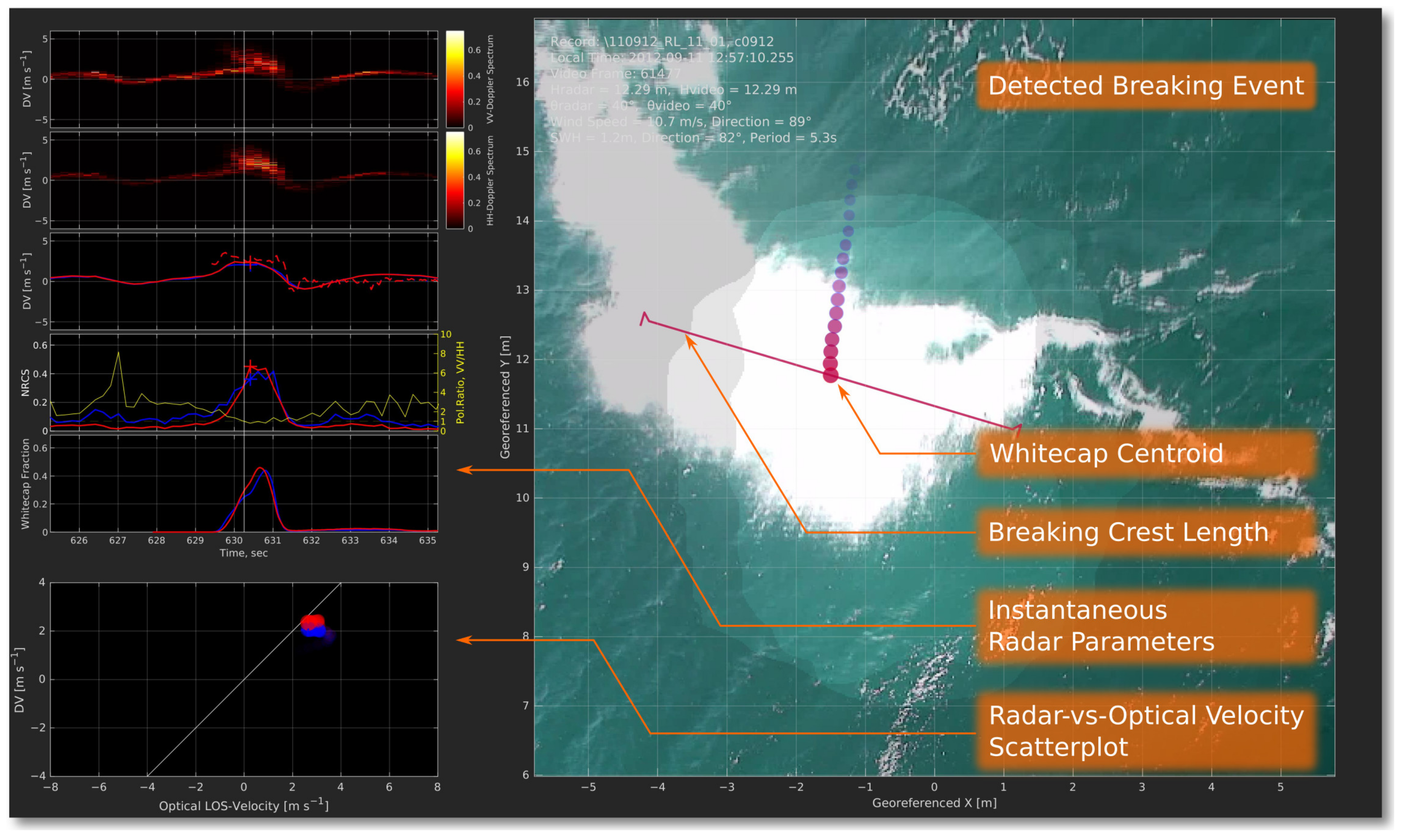
An example of joint radar–video processing. The (left) plots show the instantaneous VV, HH Doppler spectra, instantaneous Doppler velocity (DV), breaker optical line-of-sight velocity (LOV), VV and HH footprint RCS and their ratio, footprint fraction covered by whitecaps, and scatterplot between DV and LOV (blue—VV, red—HH, yellow—VV/HH-ratio). The (right) image shows the projected geo-referenced video frame with the detected whitecap, the time evolution of its geometric centroid points (which demonstrates the breaker trajectory and velocity; the frame rate is 25 fps), and the estimated breaking crest length. Radar footprints for VV and HH polarizations at the minus 3 dB level are shaded.
Figure 1.
An example of joint radar–video processing. The (left) plots show the instantaneous VV, HH Doppler spectra, instantaneous Doppler velocity (DV), breaker optical line-of-sight velocity (LOV), VV and HH footprint RCS and their ratio, footprint fraction covered by whitecaps, and scatterplot between DV and LOV (blue—VV, red—HH, yellow—VV/HH-ratio). The (right) image shows the projected geo-referenced video frame with the detected whitecap, the time evolution of its geometric centroid points (which demonstrates the breaker trajectory and velocity; the frame rate is 25 fps), and the estimated breaking crest length. Radar footprints for VV and HH polarizations at the minus 3 dB level are shaded.

Figure 2.
Histogram of breaker and environment characteristics for all breaking events: (a) wind speed, (b) significant wave height, (c) breaking crest speed, and (d) length.
Figure 2.
Histogram of breaker and environment characteristics for all breaking events: (a) wind speed, (b) significant wave height, (c) breaking crest speed, and (d) length.

Figure 3.
Three typical breaker records for (left column) up-wave, (middle column) cross-wave, and (right column) down-wave look geometry. (Top row) VV Doppler spectra in a linear scale with the estimated Doppler velocity (DV) and line-of-sight optical velocity (LOV); (middle row) the same as in the top row, but with Doppler spectra in the logarithmic scale; (bottom row) measured whitecap footprint fraction (blue) and polarization ratio (HH/VV, reddish). The incidence angle is 40, and the wind speed is 10 m s.

Figure 4.
Scatterplots between the measured line-of-sight optical velocity (LOV) and Doppler velocity (DV) at VV polarization for the “instant” dataset (all breaking stages) at different incidence angles: (a) , (b) , (c) , (d) , (e) , (f) , (g) , and (h) . Each point corresponds to an instantaneous video frame during a breaking event. The symbol color corresponds to the polarization ratio, HH/VV, in the logarithmic scale. Black diagonals show the lines.

Figure 5.
Scatterplots between the measured line-of-sight optical velocity (LOV) and Doppler velocity (DV) at VV polarization for the “average” dataset (with weights proportional to the whitecap footprint fraction) at different incidence angles: (a) , (b) , (c) , (d) , (e) , (f) , (g) , and (h) . Each point corresponds to a separate breaking event. The color of the symbols corresponds to the polarization ratio, HH/VV, in the logarithmic scale. The black symbols in (g) show the manual analysis data of the same dataset [52].

Figure 6.
The Doppler velocity (DV) normalized by the phase velocity of the breaking wave, , at VV polarization versus (a) the incidence angle, , for different color-coded breaker azimuths, , and (b) breaker azimuths, , for different color-coded incidence angles, . The lines indicate limiting normalized speeds: (a) and (b) .

Figure 7.
The Doppler velocity (DV) at VV polarization normalized by the breaker phase speed, , versus the breaker azimuth for different incidence angles: (a) , (b) , (c) , (d) , (e) , (f) , (g) , and (h) . Each point corresponds to a separate breaking event. The color of the symbols indicates the polarization ratio, HH/VV, in the logarithmic scale. Shaded areas show the limiting speed determined by .

Figure 8.
The Doppler velocity (DV) normalized by the line-of-sight projection of the breaker optical velocity (LOV), , versus the polarization ratio, HH/VV. The data are from the “instant” dataset and bin-averaged in 1 dB steps along the PR axis. Solid lines are the binned mean, and shaded areas are the corresponding standard deviation. Plots are color-coded versus the incidence angles.

Figure 9.
The normalized Doppler velocity, , versus the incidence angle, , for (a) VV and (b) HH polarization. The “averaged” dataset is used (each point is a separate breaking event). Cross-wave events with are excluded to avoid noise due to dividing by near-zero LOS projections. The boxplot symbols indicate the average value and standard deviation for a particular incidence angle. The thin lines indicate limiting normalized speeds corresponding to: (solid) breaking wave phase velocity—fast scatterers; (dash) breaking wave orbital velocity with -steepness—slow scatterers. The bold lines show the speculative model prediction.

Figure 10.
Sketch explaining the speculative model proposed for the experimental data’s interpretation.
Figure 10.
Sketch explaining the speculative model proposed for the experimental data’s interpretation.

Figure 11.
Photos illustrating a variety of deep-water breaking wave types observed at the Black Sea Research platform [73]: (a) up-wave view of a roller breaker, (b) cross-wave view of a breaker with a rough rear face, and (c) down-wave view of a slosh breaker with a smooth rear face. The breaking crest lengths are ∼1.5–3 m. The incidence angle is 50.


Table 1.
Dataset statistics.
| Incidence Angle () | Number of Events | Wind Speed (m s), (Mean ± Std) | Significant Wave Height (m), (Mean ± Std) | Peak Wave Period (s), (Mean ± Std) |
|---|---|---|---|---|
| 25 | 139 | 9.9 ± 2.0 | 0.87 ± 0.18 | 4.75 ± 0.37 |
| 30 | 40 | 8.1 ± 1.7 | 0.85 ± 0.07 | 4.95 ± 0.13 |
| 33 | 125 | 12.1 ± 2.0 | 0.99 ± 0.15 | 4.96 ± 0.44 |
| 35 | 99 | 7.5 ± 0.5 | 0.55 ± 0.03 | 4.38 ± 0.33 |
| 40 | 106 | 10.0 ± 2.2 | 0.99 ± 0.16 | 5.11 ± 0.37 |
| 45 | 491 | 9.3 ± 3.8 | 0.69 ± 0.21 | 5.33 ± 1.38 |
| 53 | 25 | 10.8 ± 1.2 | 0.79 ± 0.02 | 4.32 ± 0.78 |
| 55 | 56 | 12.3 ± 1.3 | 1.01 ± 0.08 | 4.93 ± 0.24 |
Table 2.
Model parameters.
| Look Direction | Face Slope, () | Surface Mean-Squared Slope, | Surface Standard Deviation, (m) |
|---|---|---|---|
| Up-wave | 0.1 | ||
| Down-wave | 0.03 |
Disclaimer/Publisher’s Note: The statements, opinions and data contained in all publications are solely those of the individual author(s) and contributor(s) and not of MDPI and/or the editor(s). MDPI and/or the editor(s) disclaim responsibility for any injury to people or property resulting from any ideas, methods, instructions or products referred to in the content. |
© 2023 by the authors. Licensee MDPI, Basel, Switzerland. This article is an open access article distributed under the terms and conditions of the Creative Commons Attribution (CC BY) license (https://creativecommons.org/licenses/by/4.0/).
Share and Cite
MDPI and ACS Style
Yurovsky, Y.Y.; Kudryavtsev, V.N.; Grodsky, S.A.; Chapron, B. On Doppler Shifts of Breaking Waves. Remote Sens. 2023, 15, 1824. https://doi.org/10.3390/rs15071824
AMA Style
Yurovsky YY, Kudryavtsev VN, Grodsky SA, Chapron B. On Doppler Shifts of Breaking Waves. Remote Sensing. 2023; 15(7):1824. https://doi.org/10.3390/rs15071824
Chicago/Turabian StyleYurovsky, Yury Yu., Vladimir N. Kudryavtsev, Semyon A. Grodsky, and Bertrand Chapron. 2023. "On Doppler Shifts of Breaking Waves" Remote Sensing 15, no. 7: 1824. https://doi.org/10.3390/rs15071824
Note that from the first issue of 2016, this journal uses article numbers instead of page numbers. See further details here.