Synergy of Sentinel-1 and Sentinel-2 Time Series for Cloud-Free Vegetation Water Content Mapping with Multi-Output Gaussian Processes

Abstract

Optical Earth Observation is often limited by weather conditions such as cloudiness. Radar sensors have the potential to overcome these limitations, however, due to the complex radar-surface interaction, the retrieving of crop biophysical variables using this technology remains an open challenge. Aiming to simultaneously benefit from the optical domain background and the all-weather imagery provided by radar systems, we propose a data fusion approach focused on the cross-correlation between radar and optical data streams. To do so, we analyzed several multiple-output Gaussian processes (MOGP) models and their ability to fuse efficiently Sentinel-1 (S1) Radar Vegetation Index (RVI) and Sentinel-2 (S2) vegetation water content (VWC) time series over a dry agri-environment in southern Argentina. MOGP models not only exploit the auto-correlations of S1 and S2 data streams independently but also the inter-channel cross-correlations. The S1 RVI and S2 VWC time series at the selected study sites being the inputs of the MOGP models proved to be closely correlated. Regarding the set of assessed models, the Convolutional Gaussian model (CONV) delivered noteworthy accurate data fusion results over winter wheat croplands belonging to the 2020 and 2021 campaigns ($NRMS{E}_{wheat2020}$ = 16.1%; $NRMS{E}_{wheat2021}$ = 10.1%). Posteriorly, we removed S2 observations from the S1 & S2 dataset corresponding to the complete phenological cycles of winter wheat from September to the end of December to simulate the presence of clouds in the scenes and applied the CONV model at the pixel level to reconstruct spatiotemporally-latent VWC maps. After applying the fusion strategy, the phenology of winter wheat was successfully recovered in the absence of optical data. Strong correlations were obtained between S2 VWC and S1 & S2 MOGP VWC reconstructed maps for the assessment dates (${\overline{R^2}}_{wheat-2020}$ = 0.95, ${\overline{R^2}}_{wheat-2021}$ = 0.96). Altogether, the fusion of S1 SAR and S2 optical EO data streams with MOGP offers a powerful innovative approach for cropland trait monitoring over cloudy high-latitude regions.

1. Introduction

Remote sensing (RS) technology offers an appealing opportunity to continuously quantify the health and productivity of croplands [1,2]. One of the key elements that significantly affect crop productivity is water [3]. Sufficient water availability is necessary for proper plant growth, nutrient uptake, and photosynthesis. Vegetation water content (VWC) is a useful indicator of the water status of crops and can help in monitoring the water needs and ensuring optimal management [4,5,6]. Climate change has become more pronounced over the past few decades and has caused water scarcity in many regions of the world. Consequently, water stress manifested as among the most critical abiotic stressors, negatively affecting plant growth and crop yield worldwide [7]. Real-time monitoring of the plant water status is urgently required to enable effective management of irrigation scheduling and to prevent waste of water and crop stress. Leaf water content (LWC) is a key variable for vital physiological processes, such as stomatal conductance and transpiration [8]. However, decoupling the spectral contributions of LWC and vegetation’s canopy is challenging. Instead, the estimation of VWC, described by LWC × LAI, is more feasible and often preferred [9].

Today, an unprecedented amount of Earth observation (EO) opportunities emerged from the advent of the European Space Agency’s Copernicus programme [10]. The Sentinels satellites guarantee long-term observational commitment and operate a variety of sensors with different spectral configurations and spatial resolutions offering global coverage and synergistic data exploiting possibilities [10]. The flagship land optical operational EO system is the Sentinel-2 (S2) constellation consisting of two polar-orbiting satellites (S2-A and S2-B) [11]. The multi-spectral instrument (MSI) on board S2, combines a relatively high spatial resolution (10–20 m) with a good spectral resolution (13 bands), and the combination of the two satellites ensures a high revisit time (5-day). A remarkable amount of research applying S2 data for crop traits mapping in a quantitative way has been successfully conducted [12,13,14,15,16]. Beyond the well-known benefits that optical RS provides for cropland monitoring, the retrieval of complete vegetation traits time series along the phenological cycle is sometimes hampered by weather conditions in high-latitude areas. In this regard, radar-based RS brings the technology to mitigate this limitation. Sentinel-1 (S1) as a synthetic aperture radar (SAR) sensor permits C-band image acquisition in all-weather conditions during day or night time [17]. The S1 constellation, comprising of S1-A and S1-B satellites, predefines the interferometric wide swath (IW) mode over land consisting of dual-polarized (VV & VH) images, at 10 m of spatial resolution every 6 days in a single pass. Although there is consensus that the vegetation-radar backscatter mechanisms are complex, there is no doubt that the radar signal at C-band is altered by the vegetation’s three-dimensional structure and biomass [18,19]. Unlike optical satellites, the observation geometry plays a weighty role in radar acquisitions [20,21]. Multiple studies exploited radar imagery for vegetation biophysical variables monitoring [22,23,24,25]. For instance, Caballero et al. [25] presented a novel approach based on S1 radar observations at different local incidence angles for winter wheat LAI monitoring. They achieved satisfactory validation results ($R^2$ = 0.67 and RMSE = 0.88 m${}^2$ m${}^{-2}$), and proved that S1-based LAI predictions can support cropland monitoring in cloud-prone areas where the optical vegetation traits retrieval models cannot be applied for quantitative crop mapping purposes.

The frequent coverage and the systematic observations of S1 & S2 have opened the door to data-fusion-based RS applications for crop monitoring, land surface change detection and land cover mapping [26,27]. Several research efforts took advantage of the high radiometric quality of S1 in synergy with the improved optical sensor of S2 [28,29,30,31]. However, processing S2 optical and S1 radar time series has always been tedious, particularly when a substantial number of preprocessing steps must be implemented for the whole dataset. Downloading S1 and S2 images from the Copernicus data hub [32] usually requires a lot of time and storage space. In this regard, seeking to achieve fully automated preprocessing of EO data streams, migration to cloud-computing platforms offers a solution [33]. Recently, the Google Earth Engine (GEE) platform emerged as a promising, free-access, high-performance computing platform that enables cloud-based processing of petabytes of S1 and S2 satellite data, among others [34]. The GEE platform not only provides the powerful computational capability and access to the Copernicus catalog, but also allows for the integration of machine learning (ML) algorithms [33,35].

Regarding the creation of continuous, cloud-free S1 & S2 time series data streams, ML techniques can be implemented to explicitly learn and exploit the joint relationships of both data streams. Gaussian processes (GP), a nonparametric Bayesian ML regression algorithm, has had a notable impact on the remote sensing community following the pioneering publication by Rasmussen and Williams [36]. GP has been openly and successfully applied for the learning task of analyzing the auto-correlations of single-EO-dataset-channel models [33,37]. GP regression has advanced considerably in recent years, extending the GP concept to multiple-channel models. For computing non-trivial dependencies between multiple and related model outputs, multi-task Gaussian process prediction [38] widely known as multi-output Gaussian process (MOGP) offers a set of kernel models to learn such correlations [39]. The concept of multi-output learning emerged from the field of geostatistics [40]. The MOGP modeling approach can capture valuable information across correlated outputs to provide more accurate predictions than directly modeling these outputs independently [41]. In the context of EO data streams, developing models that exploit the dependencies between optical and radar sensors results particularly convenient when the optical data are affected by cloudy sky conditions leading to gaps in the data stream. Thus, SAR imagery can be used to complement optical sources [29,33,42]. A differentiating attribute of MOGP is the ability of the models to perform multiple channel prediction tasks in the presence of missing input data [43]. This makes MOGP particularly appealing for the fusion of S1 and S2 data streams.

To date, the usage of MOGP to fuse S1 and S2 data streams has only been investigated by Pipia et al. [29] with the purpose of producing continuous LAI time series. Radar-optical data fusion for crop monitoring purposes is a novel field of research that warrants greater attention. For instance, the synergistic usage of S1 & S2 data streams for crop monitoring in a cloud-computing platform by exploiting the cross-correlations of the MOGP model’s output channels have yet to be fully explored. Therefore, this study aims to fulfill the following three main objectives: (1) to train several MOGP models with S1 radar vegetation index (RVI) [44] & S2 GP VWC time series data over two irrigated winter wheat paddocks and select the best model for posterior data fusing; (2) to examine if the best-performing MOGP model effectively retrieves crop traits under simulated cloudy conditions; (3) to map the S1 & S2 MOGP-reconstructed VWC values for the gap-filled intervals at the pixel level and evaluate the MOGP’s capacity for reconstructing the complete phenological cycle of winter wheat in the absence of optical data.

2. Methodology

2.1. Theoretical Background

In the following, we notationally review the single-output GP and MOGP formulations, adapted to the general requirements of this study.

2.1.1. Single-Output Gaussian Processes Modeling

We refer to the standard GP as a single-output Gaussian process (SOGP). It can be formulated as follows. Let $\mathfrak{D}={\left\{x_i,y_i\right\}}_{i=1}^N$, be a set of N pairs of a $x_i$∈${\mathbb{R}}^{\mathcal{B}}$ point belonging to the training dataset $X={\left\{x_i\right\}}_{i=1}^N$ assigned to a random variable $y_i$. GP is a random process that uses these pairs to learn the function outputs $f_{*}$ given a test dataset $X_{*}$ of size $N_{*}\times \mathfrak{D}$. Let us assume an additive noise model with a zero mean:

$$y_i=f_i\left(x_i\right)+{\mathcal{E}}_i,{\mathcal{E}}_i\sim \mathcal{N}\left(0,{\sigma }_n^2\right)$$

(1)

where ${\sigma }_n^2$ is the variance of the Gaussian noise and $f_i$ is the nonparametric latent function to be found. Assuming independent Gaussian noise, the joint distribution of observations and test predictions is:

$$\left(\begin{array}{c}y\\ f_{*}\end{array}\right)\sim \mathcal{N}\left(\left[\begin{array}{c}0\\ 0\end{array}\right],\left[\begin{array}{cc}\mathit{K}\left(X,X\right)+{\sigma }_n^2\mathit{I}& \mathit{K}\left(X,X_{*}\right)\\ \mathit{K}\left(X_{*},X\right)& \mathit{K}\left(X_{*},X_{*}\right)\end{array}\right]\right)$$

(2)

where $K\left(X,X\right)$ represents the self-similarities in the training set, $K\left(X,X_{*}\right)=K_{*}$ and $K\left(X_{*},X\right)=K_{*}^T$ are the similarities between training and test sets, and $K\left(X_{*},X_{*}\right)=K_{**}$ express the self-similarities in the test set. SOGP models are built through parametrizing a covariance kernel that computes the measures of similarity between two points $x_i$ and $x_j$. Expressive kernels allow the improved representation of complex signals. The squared exponential kernel arises as one of the most used kernels in GP modeling. It can be calculated as:

$$k\left(x_i,x_j\right)={\sigma }_f^2{e}^{-\frac{1}{2{\ell }^2}{∥x_i-x_j∥}^2}$$

(3)

where ${\sigma }_f^2$ (signal variance) is a scaling factor, and parameter ℓ (variance of the Gaussians) controls the length scale that modules the regression process smoothness and confidence. The model hyperparameters can be learned by maximizing the marginal likelihood of the model [45], through a cross-validation strategy [46], or applying a Bayesian learning process [47]. A SOGP establishes a prior distribution over functions. This can be converted to a posterior probability distribution of $X_{*}$ given f and the previous X conditioning on the observations, to obtain another Gaussian:

$$p\left(f_{*}|X_{*},X,y\right)\sim \mathcal{N}\left(y_{*}|{\mu }_{SOGP},{\sigma }_{SOGP}^2+{\sigma }_n^2\mathit{I}\right)$$

(4)

According to the SOGP formulation, $f_{*}$ is normally distributed with mean (${\mu }_{SOGP}$) and variance (${\sigma }_{SOGP}^2$) given by:

$${\mu }_{SOGP}\left(x_{*}\right)=k\left(x_{*},X\right){\left[\mathit{K}\left(X,X\right)+{\sigma }_n^2\mathit{I}\right]}^{-1}y$$

(5)

$${\sigma }_{SOGP}^2\left(x_{*}\right)=k\left(x_{*},x_{*}\right)-k\left(x_{*},X\right){\left[\mathit{K}\left(X,X\right)+{\sigma }_n^2\mathit{I}\right]}^{-1}k\left(X,x_{*}\right)$$

(6)

To sum up, SOGP offers a natural mechanism to construct and calibrate uncertainties automatically.

2.1.2. Multi-Output Gaussian Processes Modeling

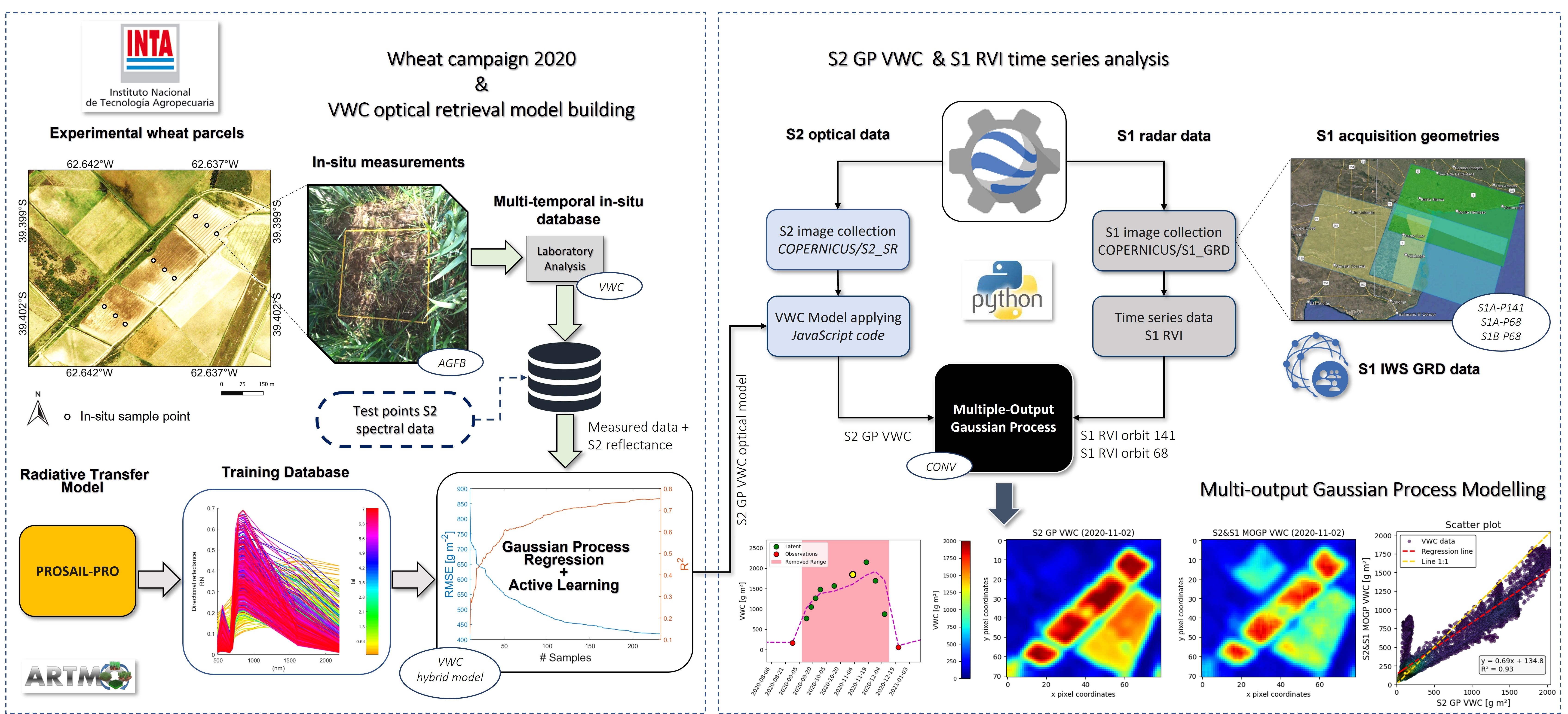
Let us now assume the S1 and S2 synergy case, where different outputs have different training input points, this model is called heterotopic in the geostatistics literature [48]. For simplicity, we assume an isotopic setting where each model output has the same set of inputs. In the following, we assume that the mean vector of the Gaussian distribution is zero in a free-noise environment. Let ${\mathfrak{D}}_1=\left\{\left(t_i,f_1\left(t_i\right)\right)|i=1,\dots ,N\right\}$ be a set of N pairs of RVI random functions $f_i$ extracted from S1 SAR data acquired at times $t_i$ and ${\mathfrak{D}}_2=\left\{\left(t_i,f_2\left(t_i\right)\right)|i=1,\dots ,N\right\}$ the corespondent VWC samples derived from S2 optical data, if $f_1$ and $f_2$ follow a GP we can write:

$$f_1\left(t\right)\sim \mathcal{GP}\left(0,k_1\left(t,t_{*}\right)\right)$$

(7)

$$f_2\left(t\right)\sim \mathcal{GP}\left(0,k_2\left(t,t_{*}\right)\right)$$

(8)

where $k_1$ and $k_2$ are the covariance kernels then the vector valued functions for $f_1$ and $f_2$ can be expressed as Gaussian distributions $f_1\sim \mathcal{N}\left(0,{\mathit{K}}_1\right)$ and $f_2\sim \mathcal{N}\left(0,{\mathit{K}}_2\right)$ being $K_1$ and $K_2$ the covariance kernel matrixes. Now we create a stacked larger vector $\mathit{f}$ containing $f_1$ and $f_2$. Assuming that the two processes are independent we can obtain:

$$\left[\begin{array}{c}{f}_1\\ f_2\end{array}\right]\sim \mathcal{N}\left(\left[\begin{array}{c}0\\ 0\end{array}\right],\left[\begin{array}{cc}{\mathit{K}}_{\mathit{1}}& \mathbf{0}\\ \mathbf{0}& {\mathit{K}}_{\mathbf{2}}\end{array}\right]\right)$$

(9)

where the blocks outside the main diagonal are zero because the dependency between $f_1$ and $f_2$ was supposed to be zero. The easiest way to extend the SOGP to MOGP cases is to model each of the model’s channels singly with a SOGP. If the outputs are correlated, the SOGP approach fails to account for correlations between the outputs of the model impairing regression processes performance [38]. If we want to account for dependencies between the processes, the joint multivariate Gaussian distribution can be written as:

$$\left[\begin{array}{c}{f}_1\\ f_2\end{array}\right]=\left[\begin{array}{c}{f}_1\left(t_1\right)\\ ⋮\\ f_1\left(t_N\right)\\ f_2\left(t_1\right)\\ ⋮\\ f_2\left(t_N\right)\end{array}\right]\sim \mathcal{N}\left(\left[\begin{array}{c}0\\ 0\end{array}\right],\left[\begin{array}{cc}{\mathit{K}}_{{\mathit{f}}_{\mathbf{1}},{\mathit{f}}_{\mathbf{1}}}& {\mathit{K}}_{{\mathit{f}}_{\mathbf{1}},{\mathit{f}}_{\mathbf{2}}}\\ {\mathit{K}}_{{\mathit{f}}_{\mathbf{2}},{\mathit{f}}_{\mathbf{1}}}& {\mathit{K}}_{{\mathit{f}}_{\mathbf{2}},{\mathit{f}}_{\mathbf{2}}}\end{array}\right]\right)$$

(10)

Equation (10) can be simplified to $f\sim \mathcal{N}\left(0,{\mathit{K}}_{\mathit{f},\mathit{f}}\right)$. The main challenge of MOGP is to build a cross-covariance function $cov\left[f_1\left(t\right),f_2\left(t_{*}\right)\right]$ such that the matrix ${\mathit{K}}_{\mathit{f},\mathit{f}}$∈${\mathbb{R}}^{NxN}$ is positive semi-definite and symmetric [39,41]. The properties of the SOGP are immediately transferred to MOGP because it can straightforwardly be interpreted as SOGP on an extended input space. For a detailed review of the ${\mathit{K}}_{\mathit{f},\mathit{f}}$ matrix development see the publication by Álvarez et al. [39].

One particular approach for building the covariance functions is known as process convolution. Each output of the model results from the convolution of a smoothing kernel and a latent random GP. It was firstly introduced by Barry and Hoef [49] to construct covariance functions for SOGP, and later for MOGP [50,51].

2.2. Study Area

The Region of Interest (ROI) selected for the study is an irrigated crop area located in Buenos Aires Province, in the southeast of Argentina (see Figure 1). The extension of the cultivated area of the Bonaerense Valley of Colorado River (BVCR) is approximately 91,163 ha, comprising winter crops such as wheat, barley, forage, and cereals and horticulture [52]. Since 2016, a team of experts from Argentina’s National Institute of Agricultural Technology (INTA) Hilario’s Ascasubi Experimental Station (HAEE) has been gathering in situ data to create a land cover map each year [25]. The appointed study area mainly corresponds to a dryland agri-environment, and gravity irrigation has enabled most of the agricultural practices in the region [53]. This study focused on two winter wheat fields (triticum aestivum) belonging to the BVCR’s 2020 and 2021 crop campaigns [54].

2.3. Sentinel-2 Time Series Preprocessing

The COPERNICUS/S2_SR image collection over the ROI was assembled using GEE, where the S2 multispectral surface reflectance (S2-L2A) images are available in the form of tiles from December 2018 to current. The cloudy pixel percentage (CPP) was configured to 5 % and the bitmask QA60 band with cloud mask information was used to filter the S2 image collection. The cloud mask permits cloudy and cloud-free pixels to be identified. The 60 m resolution QA60 band includes both cirrus clouds and dense clouds with an indicator specifying the cloud type. Bits 10 and 11 are clouds and cirrus, respectively. The standard GP regression model presented in Caballero et al. [54] was tailored to be scalable into the GEE framework to generate VWC time series at 10 m using the methodology proposed by Pipia et al. [33]. The S2 GP VWC hybrid model was trained with in situ measurements collected in the BVCR during the 2020 crop campaign using Gaussian Processes as a core machine learning regression algorithm (MLRA) and an active learning technique (AL) [55] to estimate VWC of irrigated winter wheat (R${}^2$ = 0.75, RMSE = 416 g m${}^{-2}$). With AL strategies, the number of samples in hybrid modeling can be effectively decreased. Therefore, using an “optimal” statistical technique, the MLRA selects the most representative samples from the training dataset, which leads to the GP hybrid model reaching superior accuracies [56]. Several research efforts have successfully used AL to intelligently reduce the training dataset’s size [54,57,58,59]. The in situ VWC values considered the total amounts of water stored in all wheat plant organs including leaves, fruits, flowers, and stalks. The VWC values were then obtained by calculating the difference between the fresh (FW) and dry (DW) organic matter and referring it to the sowing area (A) implicated in the field data collection process. Additionally, seeking to integrate the bare soil contribution, we introduced the fractional vegetation cover (FVC) in situ measured values to the calculations of VWC:

$$VWC=\frac{\left(FW-DW\right)}{A}\times FVC\left[g{m}^{-2}\right]$$

(11)

FVC is defined as the ratio of green vegetation’s vertical projected area to the considered land surface extension [60,61,62,63,64]. This approach arises as a necessity for the improvement of the concept of canopy water content (CWC) defined as the total mass of water in all plants’ leaves per surface unit (see Section 2.5.1 of Caballero et al. [54] for a thorough explanation of the formulas used to determine the VWC values). The S2 GP VWC hybrid model accepts as input the S2 spectral bands at 10 m and 20 m and predicts VWC along with associated uncertainties. The availability of S2 images strongly depends on sky conditions over the study site and differs from one crop campaign to other. A total of 44 and 52 cloud-free atmospherically corrected S2 scenes were collected unequally spaced between December 2018 and January 2021 (11 S2 images correspond to the winter wheat 2020 crop campaign from 29 August to 12 December 2020) (see also Caballero et al. [54] for details), and between November 2019 and January 2022 (8 S2 images correspond to the winter wheat 2021 crop campaign from 24 August to 22 December 2021), respectively.

2.4. Sentinel-1 Time Series Preprocessing

Only descendent orbits were found suitable for monitoring the ROI due to the S1 acquisition configuration over the study site. Two relative orbits are thus available for EO purposes: orbits 68 for S1-A and S1-B and 141 for S1-A. A detailed overview of the S1 acquisition over the BVCR at multiple incidence angles is provided by Caballero et al. [25]. In the case of S1, the acquisitions are equally spaced. One S1-A or S1-B descendent pass is available every 6 days over the study site for the relative orbit 68 approximately at 6.20 a.m. local time. The S1-A acquisitions for the relative orbit 141 have a revisit time of 12 days. Radar data was collected from the GEE catalog accessing the COPERNICUS/S1_GRD_FLOAT dataset. It provides S1 Interferometric Wide Swath (IW) Ground Range Detected (GRD) scenes in dual-polarization VH+VV, that have been processed using the Sentinel-1 Toolbox to generate radiometrically calibrated, ortho-corrected products. For each BVCR crop campaign, two completed collections of S1 images were created for the two observation geometries, covering a time span of more than 3 years. From December 2018 to January 2021, there were 64 S1–orbit 141 and 103 S1–orbit 68 images (21 S1–orbit 68 images and 11 S1–orbit 141 images correspond to the 2020 winter wheat crop campaign) and 66 S1–orbit 141 and 115 S1–orbit 68 images from November 2019 to January 2022 (21 S1–orbit 68 images and 10 S1–orbit 141 images correspond to the 2021 winter wheat crop campaign). For each S1 scene, the dual-pol Radar Vegetation Index (RVI) Kim et al. [44], was initially generated as follows:

$$RVI=\frac{4VH}{VH+VV}$$

(12)

The coherent integration of signals backscattered from different targets in the resolution cell induces the speckle noise to be generated in the S1 data. The use of local statistics is one of the simplest ways to reduce the speckle noise in SAR data [65]. Spatial speckle filtering 7 × 7 Refined Lee [66] as coded in https://github.com/senbox-org/s1tbx/ (accessed on 11 January 2023), was applied. The refined Lee approach makes use of local gradient data. It does not blur the edges and minute details, and it does not require picture modeling. Depending on how the edge is oriented, the local mean and variance for both the additive and multiplicative noise instances are calculated from a smaller number of pixels. As a result, the edge becomes sharper and the noise around it is reduced [66]. Veloso et al. [28] analyzed the temporal trend of the cross-polarized ratio VH/VV for a variety of winter and summer crops (wheat, rapeseed, maize, soybean and sunflower) in southwest France. They suggested a 7 × 7 window size for filtering the speckle of the cultivated region observed by S1. To recover the essential curve shape, S1 time series smoothing is required [67]. Smoothing has the dual objectives of removing random noise and, ideally, maintaining the true spectral signal. For signal denoising purposes, RVI temporal profiles were filtered using an additional Savitzky–Golay (S–G) smoother [68] (window length = 9, polynomial order = 2) at the pixel level. The S–G smoother whit these predefined parameters, fits a polynomial of order 2 to the 9 RVI samples in the window length to locally smooth a noisy signal employing the least-squares concept. Regarding the S–G parametrization, lower values of the polynomial order can cope with low-rate changing phenomena such as crop rotation in the BVCR. The size of the windows is related to the frequency of the S1 acquisitions. The S–G parameters selection methodology was based on the analysis of the power spectrum associated with the S1–RVI signal. High-frequency components in the power spectrum result from the noise’s (if it’s genuinely random) ability to shift unpredictably from pixel to pixel. On the other hand, the lower frequency range has a greater concentration of signal power [69].

2.5. MOGP Models Parametrization

The MOGP processing was entirely conducted within the Multi-Output Gaussian Process Toolkit (MOGPTK) [43] version 0.3.2. The MOGPTK is a Python toolkit for performing multi-output GP regression with kernels utilizing the cross-correlation information between channels to better model time-series signals. The set of MOGP kernels implemented is particularly pertinent for signal reconstruction in the case of missing data. The toolkit provides the functionality for training and interpreting GP models with multiple data channels and includes plotting functions for the case of single input with multiple outputs. More information can be found at: https://github.com/GAMES-UChile/mogptk/ (accessed 11 January 2023).

The preprocessed S1 and S2 time series were first loaded into MOGPTK creating two and three-channel models: (i) S2 GP VWC (CH-1), (ii) S1 orbit 68 RVI (CH-2), (iii) S1 orbit 141 RVI (CH-3). Then we removed a range of data from the CH-1 to simulate the S2 data loss corresponding to the winter wheat cycles (From the beginning of September to the end of December, we removed 9 S2 images for the 2020 campaign and 6 S2 scenes related to the 2021 winter wheat crop campaign) and additionally removed 10% of the data points for CH-2 and CH-3 randomly. Regarding 2020 and 2021 crop campaigns, 35 S2 (CH-1) + 92 S1–orbit 68 (CH-2) + 53 S1–orbit 141 (CH-2) images and 46 S2 (CH-1) + 103 S1–orbit 68 (CH-2) + and 59 S1–orbit 141 (CH-3) images were synergistically used to train the MOGP models, respectively. Aiming to improve training results each data channel was linearly detrended and normalized to have zero mean and unit variance utilizing the transformations provided by the MOGPTK. We analyzed four MOGP spectral kernels: (i) the Spectral Mixture Kernels for Multi-Output Gaussian Processes (MOSM) [70], (ii) the Cross-Spectral Mixture (CSM) [71], (iii) the Linear Model of Coregionalization (LMC) [39,40], and (iv) the Convolutional Model (CONV) [72,73] with four spectral components per channel (Q = 4). The MOGP kernels’ parameters were randomly instantiated to establish an initial set of reasonable values for the S1 & S2 dataset using Independent Spectral Mixture (SM) as an estimation method. SM fits an independent GP model for each channel of the dataset with a spectral mixture kernel. Posteriorly it uses the tuned parameters as initial values of the MOGP kernels. For each channel, the noise was initialized with 1/30 of the variance. The MOGP models were then trained using the Adam optimizer [74]. During the training stage, the hyperparameters of the kernel are optimized to approach the training data. The learning rate was set up to 0.1 and the number of iterations for initialization in 500.

In addition, we also considered the SOGP SM kernel using the Bayesian Nonparametric Spectral Estimation (BNSE) [75] as the initialization method to estimate the kernel parameters from the S1 & S2 dataset. BNSE aims to assess the power spectral density of a time series signal and then select the Q greater peaks in the estimated spectrum. The kernel’s mean, magnitude, and variance are initialized based on the peak’s position, magnitude, and with of the detected spectral components, respectively.

2.6. Experimental Setup

Two distinct ROIs were considered for training the MOGP algorithms and evaluating the S1 and S2 synergy capacity to map VWC over an irrigated area of winter wheat crop.

Table 1. ROI boundaries in geographic coordinates (WGS84), x-pixels quantity (Qty-x), y-pixels quantity (Qty-y), and ROI area selected for training the MOGP models with the S1 & S2 dataset. ROI-1 belongs to the winter wheat 2020 site whereas the ROI-2 to 2021 site.

	North	West	South	East	Qty-x	Qty-y	Area [ha]
ROI-1	−39.398	−62.645	−39.404	−62.636	10	12	1.2
ROI-2	−39.391	−62.618	−39.392	−62.616	12	13	1.56

shows the geographic boundaries, the dimension in pixels, and the area expressed in hectares for each selected ROI belonging to the winter wheat paddocks of the BVCR 2020 and 2021 crop campaigns. The S2 GP VWC maps were stacked along with S1 orbit 68 and S1 orbit 141 RVI products and the mean for the ROI was then calculated. An exhaustive detail of S1 & S2 acquisition dates for models validation corresponding to the winter wheat 2020 and 2021 crop campaigns is given in

Table A1. Sentinel–2 and Sentinel–1 acquisition dates corresponding to the winter wheat 2020 crop campaign at the BVCR. The (–) symbol means no acquisition. The (*) indicates the S2 removed images from the S1 & S2 dataset for model validation.

Winter Wheat 2020 Crop Campaign
S2 Acquisition Date	S1(Orbit 68) Acquisition Date	S1(Orbit 141) Acquisition Date
-	2020-08-27	-
2020-08-29	-	-
-	-	2020-09-01
-	2020-09-02	-
2020-09-13 *	-	2020-09-13
2020-09-18 *	-	-
-	2020-09-20	-
2020-09-23 *	-	-
-	-	2020-09-25
-	2020-09-26	-
2020-09-28 *	-	-
-	2020-10-02	-
-	-	2020-10-07
-	2020-10-08	-
2020-10-13 *	-	-
-	2020-10-14	-
-	-	2020-10-19
-	2020-10-20	-
-	2020-10-26	-
-	-	2020-10-31
-	2020-11-01	-
2020-11-02 *	-	-
-	2020-11-07	-
-	-	2020-11-12
-	2020-11-13	-
2020-11-17 *	-	-
-	2020-11-19	-
-	-	2020-11-24
-	2020-11-25	-
2020-11-27 *	-	-
-	2020-12-01	-
-	-	2020-12-06
2020-12-07 *	2020-12-07	-
-	2020-12-13	-
-	-	2020-12-18
-	2020-12-19	-
2020-12-22	-	-
-	2020-12-25	-
-	-	2020-12-30
-	2020-12-31	-
-	2021-01-06	-

and

Table A2. Sentinel–2 and Sentinel–1 acquisition dates corresponding to the winter wheat 2021 crop campaign at the BVCR. The (–) symbol means no acquisition. The (*) indicates the S2 removed images from the S1 & S2 dataset for model validation.

Winter Wheat 2021 Crop Campaign
S2 Acquisition Date	S1(Orbit 68) Acquisition Date	S1(Orbit 141) Acquisition Date
-	2021-08-16	-
-	2021-08-22	-
2021-08-24 *	-	-
-	-	2021-08-27
-	2021-08-28	-
-	2021-09-03	-
-	-	2021-09-08
-	2021-09-09	-
-	-	2021-09-20
-	2021-09-21	-
-	2021-09-27	-
-	-	2021-10-02
2021-10-03 *	2021-10-03	-
2021-10-08 *	-	-
-	2021-10-09	-
-	-	2021-10-14
-	2021-10-15	-
2021-10-18 *	-	-
-	2021-10-21	-
-	-	2021-10-26
-	-	2021-10-27
2021-11-02 *	2021-11-02	-
-	2021-11-08	-
-	2021-11-14	-
2021-11-17 *	-	-
-	-	2021-11-19
-	2021-11-20	-
-	2021-11-26	-
-	-	2021-12-01
-	2021-12-02	-
2021-12-07	-	-
-	2021-12-08	-
-	-	2021-12-13
-	2021-12-14	-
-	2021-12-20	-
2021-12-22	-	-
2022-01-01	2022-01-01	-

correspondingly. S1 & S2 datasets were used to initialize and train the MOGP models. Aiming to completely reconstruct the VWC cycles over winter wheat cropland, we created artificial S2 GP VWC data gaps (latent S2 GP VWC data). Seeking to explore the S1-derived RVI capability to reconstruct S2-based VWC maps at distinct acquisition geometries, the MOGP performance was subsequently assessed given models with two and three input channels. Three tests for each ROI were conducted analyzing the following MOGP model input configurations: (i) S2 & S1 orbit 68 (2-channel model), (ii) S2 & S1 orbit 141 (2-channel model), and (iii) (i) S2 & S1 orbits 68 and 141 (3-channel model). Several goodness-of-fit metrics were evaluated to select the best MOGP model: the mean absolute error (MAE, Equation (13)), the root mean square error (RMSE, Equation (15)), the mean absolute percentage error (MAPE, Equation (14)), the normalized root mean square error (NRMSE, Equation (16)), and the training time were recorded. Below we display the formulation used for MAE, MAPE, RMSE and NRMSE calculations:

$$MAE=\frac{1}{N}\sum _{i=1}^N|y_i-\widehat{y_i}|$$

(13)

$$MAPE=\frac{1}{N}\sum _{i=1}^N\frac{|y_i-\widehat{y_i}|}{y_i}$$

(14)

$$RMSE=\sqrt{\frac{1}{N}\sum _{i=1}^N{(y_i-\widehat{y_i})}^2}$$

(15)

$$NRMSE=\frac{RMSE}{(y_{max}-y_{min})}$$

(16)

where ${\left\{y_i\right\}}_{i=1}^N$ are the S2 GP VWC latent observations used for model assessing, ${\left\{{\widehat{y}}_i\right\}}_{i=1}^N$ are the VWC retrieved values based on S1 RVI data, $(y_{max}-y_{min})$ is the S2 GP VWC data range and $\overline{y}$ is the mean of the VWC S2-derived values. To investigate the correlation between each channel of the S1 & S2 dataset, we also plotted the cross-correlation matrix for each evaluated MOGP model. Finally, the best MOGP model was applied to winter wheat 2020 and 2021 sites (see Figure 1). A MOGP model was iteratively trained per pixel using the S1 & S2 three-channel dataset. Each S1 & S2 MOGP VWC reconstructed subset was compared against the latent S2 GP VWC by calculating the coefficient of determination (R${}^2$) and the linear regression.

2.7. Delineation of Retrieval Workflow

Figure 2 gives an overview of the complete processing workflow. Three well-defined processing blocks are depicted, starting with an S2 and S1 imagery acquisition and preprocessing section, followed by MOGP best model selection, and the retrieval of VWC applying MOGP to S1 and S2 time series datasets. To sum up, the implemented processing workflow consisted of the following six main steps:

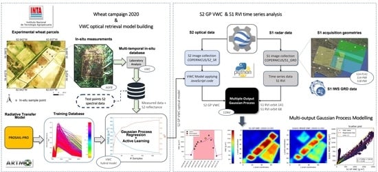
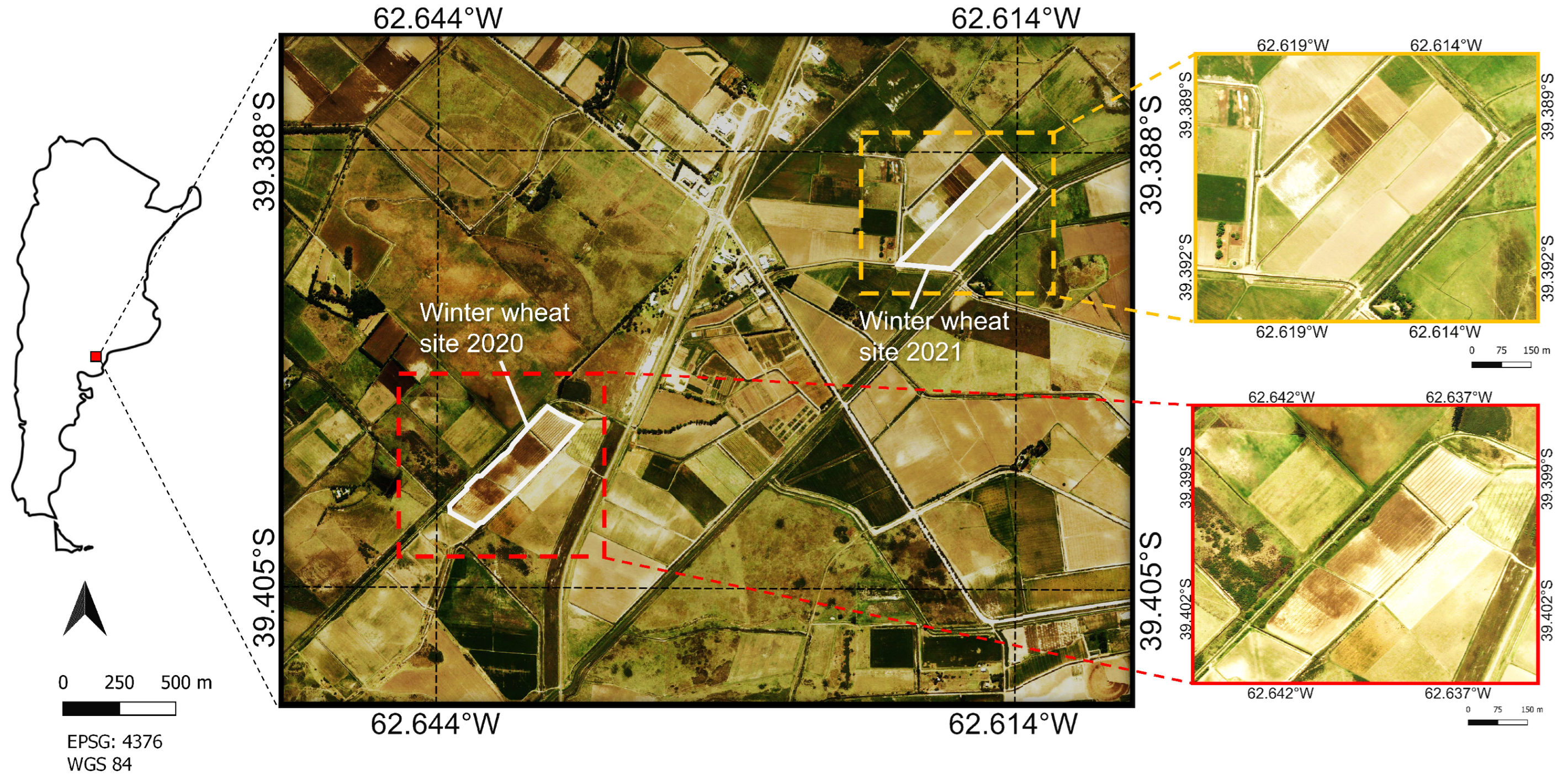
• Building of VWC time series applying a GP model trained with in situ data of the BVCR 2020 crop campaign to S2 imagery, and pre-processing of RVI time series for S1 orbit 68 and orbit 141 imagery, respectively;
• Assembling the S1 & S2 dataset containing multitemporal VWC retrieved values and S1 post-processed RVI data for a specific ROI of the BVCR study site;
• Setting up the MOGP kernels with Q = 4 and initializing the parameters using SM;
• Training the MOGP models with the S1 & S2 dataset using the Adam optimizer and assessing the regression statistics error metrics (MAE, MAPE, RMSE, and NRMSE) for best model selection;
• Multi-seasonal mapping of VWC retrieved given the best evaluated MOGP model and S1 & S2 stacked datasets at pixel level over two distinct bounded fields and corresponding process performance;
• Reconstructing of artificially removed S2 GP VWC data gaps over winter wheat cropland considering the BVCR 2020 and 2021 crop campaigns.

The entire software framework was implemented in Python version 3.6.13 (https://www.python.org/downloads/release/python-3613/, accessed on 22 September 2022) utilizing the geemap package version 0.19.1 (https://github.com/giswqs/geemap/, accessed on 11 January 2023) for mapping interactively with Google Earth Engine.

3. Results

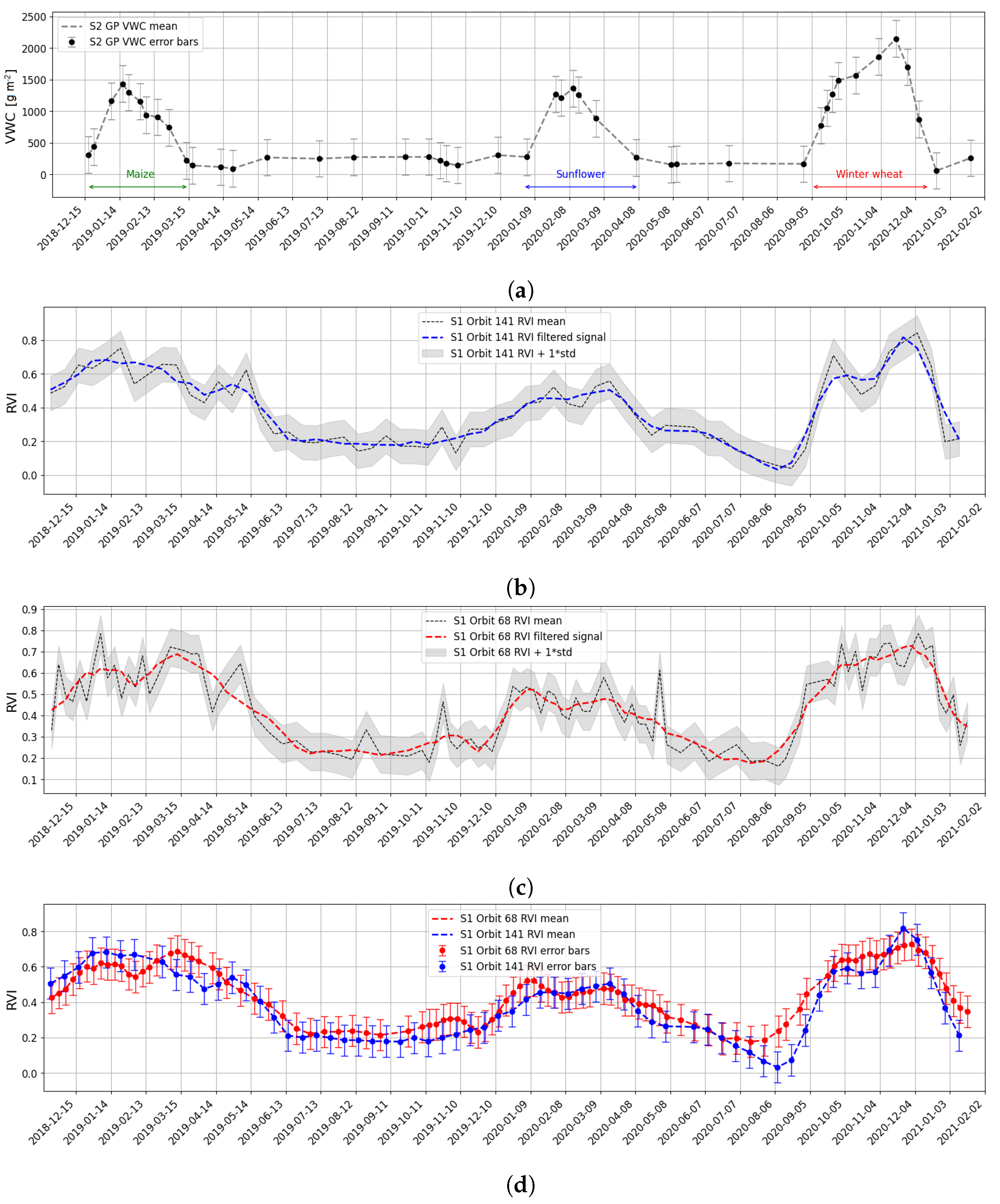
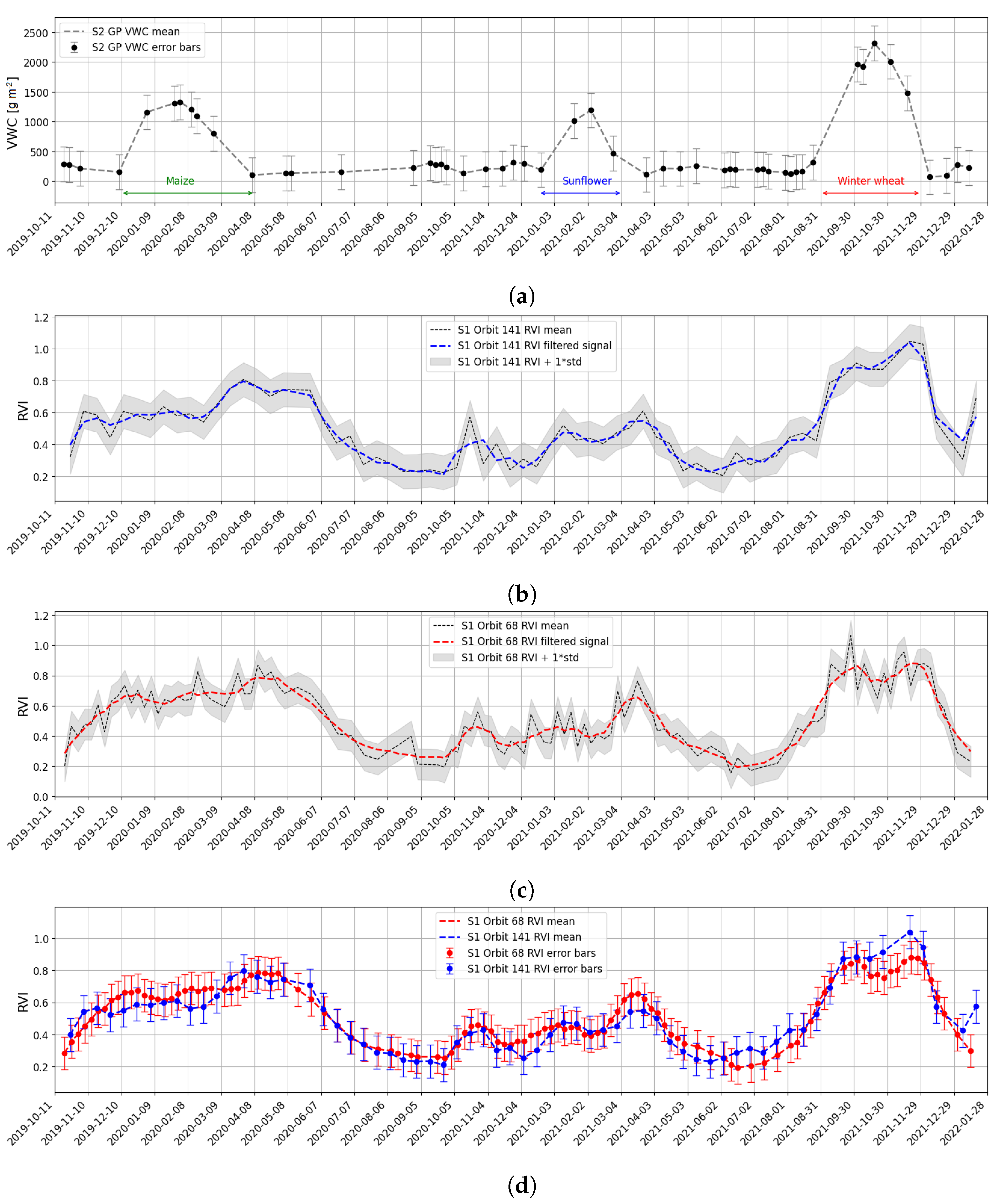
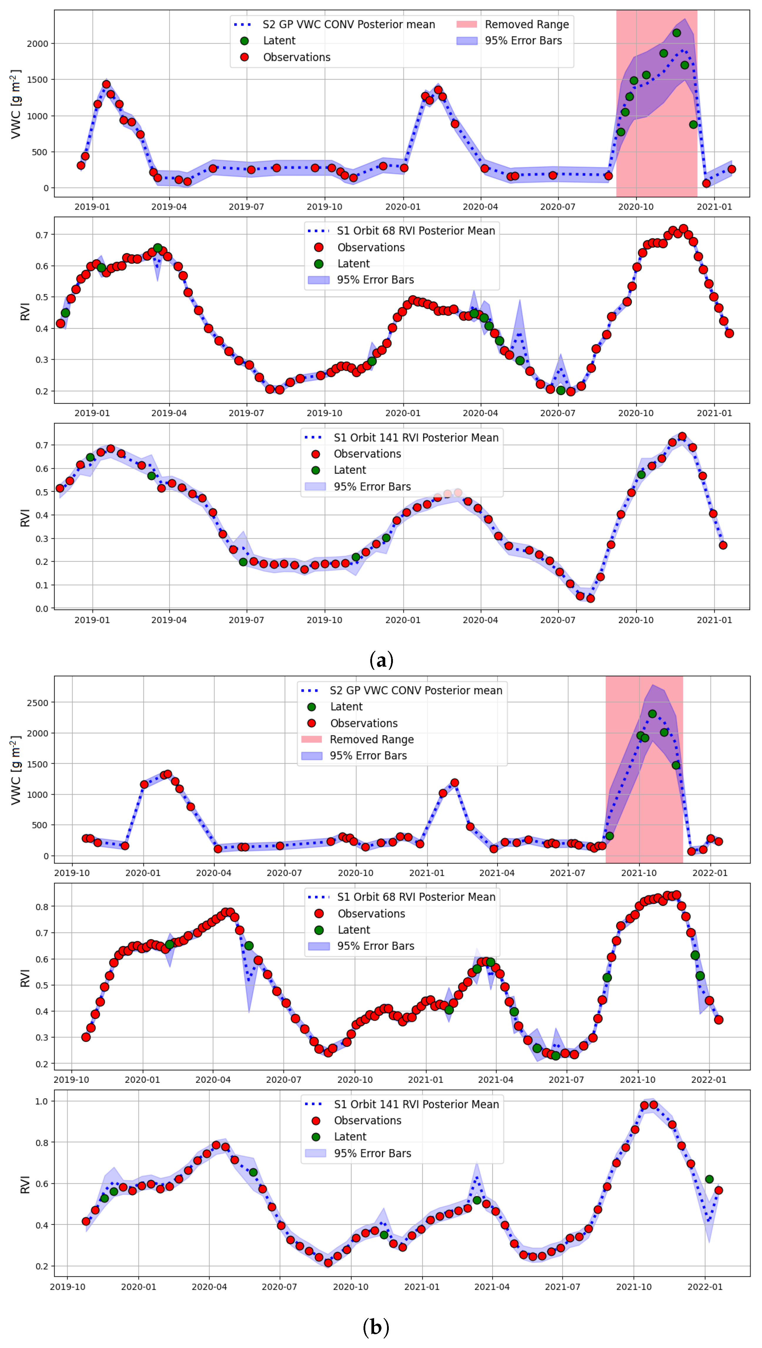
3.1. S1 SAR RVI & S2 GP VWC Temporal Profiles

In an attempt to analyze multi-seasonal VWC time series over the averaged ROI-1 presented in Table 1, the temporal profiles of S2 GP VWC and S1 RVI orbits 68 and 141 over the irrigated winter wheat sites 2020 are displayed in Figure 3. It is worth highlighting that the typical crop rotation at the study site is: maize-sunflower-wheat [53].

The temporal profiles for S2 GP VWC and S1 RVI for orbits 68 and 141 for the winter wheat 2021 averaged ROI-2 are shown in Figure 4. Regarding the winter wheat crop for the 2021 campaign, it can be seen that the summer predecessors’ crops were sunflower for hybrid seed in 2021 and maize in 2020. An appreciable difference can be distinguished when the S1 RVI for orbits 68 and 141 are plotted jointly (see Figure 3d and Figure 4d). Note that there is a time asynchrony between S1 acquisitions as both satellites S1-A and S1-B share descendent orbit 68. Moreover, the RVI amplitude offset between orbits 68 and 141 is due to the different SAR sensor’s acquisition geometry [25]. The mean local incidence angle over the study site for S1 orbit 141 is approximately 33°, whereas for orbit 68 it is around 43°.

3.2. Training MOGP Kernels for VWC Time Series Modelling

Two S1 & S2 three-channel datasets were created for training the MOGP models. We first assessed quantitatively the performance of four spectral-mixture kernels for selecting the best MOGP model and also the outcomes of SOGP to establish a ranking between them. We then explored the contribution of the S1 RVI data at two distinct descendent orbits and its effect on the MOGP models’ metrics. To do so, several trials were conducted considering 2 or 3 channels from the S1 & S2 datasets. The space of possible combinations is as follows: (a) S2 GP VWC and S1 RVI orbit 68; (b) S2 GP VWC and S1 RVI orbit 141; and (c) S2 GP VWC, S1 RVI orbit 68 and S1 RVI orbit 141.

Table 2. Error metrics and training time of the MOGP and SOGP evaluated kernels for the 2020 winter wheat averaged ROI-1.

S2 GP VWC and S1 RVI Orbit 68
MOGP Kernel	MAE [g m${}^{-2}$]	MAPE [%]	RMSE [g m${}^{-2}$]	NRMSE [%]	Time [s]
MOSM	828.85	56.42	927.56	44.34	10.58
CSM	242.7	15.43	360.55	17.24	17.85
SM-LMC	346.16	22.56	495.49	23.69	12.68
CONV	250.17	19.48	313.11	14.97	21.42
SM	881.4	58.91	1005.71	48.07	6.03
S2 GP VWC and S1 RVI orbit 141
MOSM	1025.79	69.92	1116.62	53.38	9.37
CSM	283.95	19.76	378.01	18.07	16.06
SM-LMC	482.25	31.99	580.76	27.76	11.49
CONV	255.42	25.25	419.36	20.05	19.25
SM	883.69	59.05	1009.05	48.23	4.98
S2 GP VWC, S1 RVI orbit 68 and S1 RVI orbit 141
MOSM	907.21	62.61	992.18	47.43	18.56
CSM	472.31	32.75	512.23	24.49	35.18
SM-LMC	463.04	30.75	546.85	26.14	22.67
CONV	249.3	21.83	336.74	16.1	40.27
SM	881.77	58.93	1006.25	48.1	10.29

presents the prediction statistics for the MOGP modeling when the S1 & S2 data streams are used to reconstruct time series data of VWC over the averaged BVCR 2020 winter wheat ROI-1. For each MOGP model and S1 & S2 data stream configuration, we evaluated the following error metrics: MAE, MAPE, RMSE, NRMSE and the training time.

The MOGP modeling outcomes for the 2021 winter wheat averaged ROI-2 can be visualized in

Table 3. Error metrics and training time of the MOGP and SOGP evaluated kernels for the 2021 winter wheat averaged ROI-2.

S2 GP VWC and S1 RVI Orbit 68
MOGP Kernel	MAE [g m${}^{-2}$]	MAPE [%]	RMSE [g m${}^{-2}$]	NRMSE [%]	Time [s]
MOSM	1606.97	91.26	1746.35	77.76	11.59
CSM	1420.06	79.84	1549.94	69.02	19.85
SM-LMC	1229.57	64.98	1362.06	60.65	13.9
CONV	238.07	41	328.01	14.61	22.31
SM	1408.52	75.06	1550.67	69.05	7.23
S2 GP VWC and S1 RVI orbit 141
MOSM	1606.95	91.26	1746.33	77.76	9.96
CSM	864.12	54.02	928.28	41.33	18.25
SM-LMC	1262.46	69.72	1378.87	61.4	12.24
CONV	274.33	43.77	352.11	15.68	21.78
SM	1408.52	75.06	1550.67	69.05	6.98
S2 GP VWC, S1 RVI orbit 68 and S1 RVI orbit 141
MOSM	1640.51	94.6	1778.6	79.2	21
CSM	1446.8	82.65	1576.08	70.18	36.08
SM-LMC	1395.58	74.98	1535.22	68.36	24.21
CONV	190.44	25.69	227.12	10.11	45.02
SM	1408.52	75.06	1550.67	69.05	10.2

. A linear increase in runtime can be noted when the three channels are used to train the MOGP regression models.

By eliminating S2 GP VWC samples from the S1 & S2 datasets, we artificially produced data gaps. Subsequently, we used the extracted values as a baseline for the evaluation of the MOGP models’ predictions. For that reason, from the S2 GP VWC time series in Figure 3a and Figure 4a, we deleted 9 samples from September 8 to December 12 of 2020 and 6 samples from August 19 to November 27 of 2021, which corresponds to the 2020 and 2021 complete phenological winter wheat cycles, respectively, at the study site. It is noteworthy that the number of S2 acquisitions is different for the 2020 and 2021 crop campaigns due to the cloud coverage dynamic over the study region (see Section 2.3). These latent S2 GP VWC observations exemplify realistically the cloudy image acquisition conditions of S2 at high latitudes. The MOGP regressions for the evaluated models are shown in Figure 5. The MOGP results are also compared to the SM SOGP predictions.

As observable in Figure 5, the convolutional model reaches the best results in the predictions of VWC values for both 2020 and 2021 winter wheat test sites. The complete phenological profile of the crop (green dots) is fully recovered, and all latent VWC values are predicted accurately by the CONV model in the absence of optical observations. Consequently, the CONV model is selected for the posterior task of reconstructing VWC at a pixel level. Although CSM and SM-LMC models indeed delivered good results for the 2020 winter wheat ROI, they have almost zero capacity when applied to the 2021 site. Furthermore, SOGP showed an extremely low capacity to reconstruct VWC in the artificially created gapped windows.

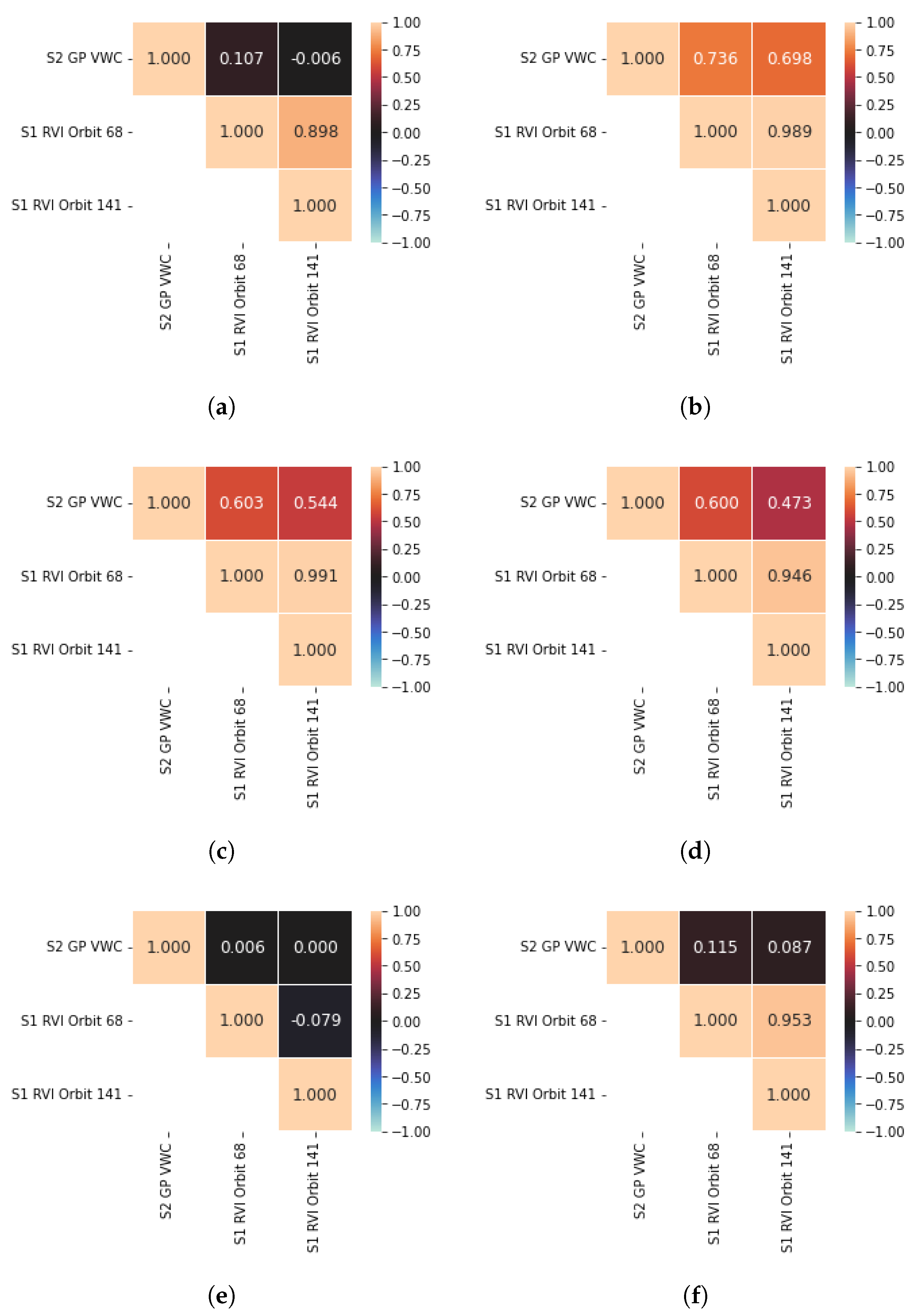
3.2.1. Cross-Correlation Matrixes for the MOGP Trained Kernels

The cross-correlation matrixes for the MOGP evaluated models over the wheat 2020 and 2021 study sites are displayed in Figure 6. The off-diagonal elements represent the dependencies between channels in the S1 & S2 dataset. These dependencies account for cross-spectral coupling among channels in the S1 & S2 dataset.

The empirical cross-correlation matrices in general terms are showing strong correlations between CH-2: S1 RVI orbit 68 and CH-3: S1 RVI orbit 141 in all cases. Nevertheless, the S1-S2 dependencies are determined by the specific MOGP kernel. In some cases CH-1: S2 GP VWC has a negligible correlation with the remaining channels.

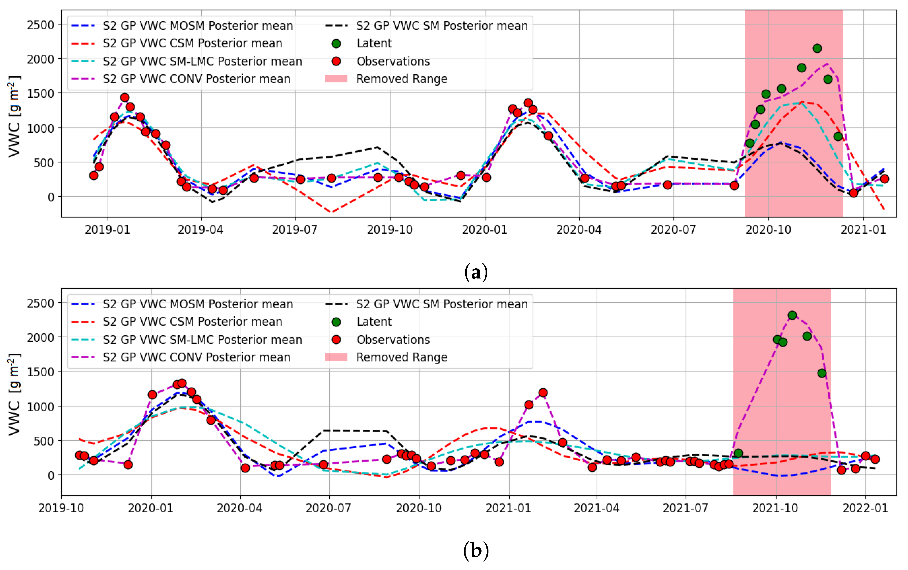
3.2.2. Optimized MOGP Kernel for Mapping the VWC of the Winter Wheat 2020 and 2021

In this section, we further explore the CONV model’s results. Figure 7 shows the CONV predictions for a three-channel trained model, the S1 & S2 dataset were fused over two different winter wheat ROIs belonging to the BVCR 2020 and 2021 campaigns. It can be noticed that the posterior mean (dashed blue line) for each channel follows the temporal trend of the original observations (red dots). The uncertainty in the form of ±$\sigma$ is represented by the limited shaded-blue area around the estimations. The S2 GP VWC and S1 RVI curves for orbits 68 and 141 follow similar behavior showing the potential of S1 RVI for crop monitoring purposes. Although the prediction uncertainty increases in the presence of latent data, our trained CONV model is able to recover the more significant trend in the VWC time series for winter wheat 2020 and 2021 minimizing the error (see Table 2 and Table 3). The S1 & S2 datasets of Figure 7 are used to optimize the hyperparameters of the CONV model for the wheat site 2020 and 2021. Their values are reported in Appendix B,

Table A3. Hyperparameters of the MOGP CONV model trained with the S2 GP VWC and S1 RVI orbits 68 and 141 time series over the winter wheat 2020 ROI-1.

Name	Range	Value
M[0].CONV.weight	($1\times {10}^{-8}$, ∞)	[0.16140878 0.12014237 0.25099972]
M[0].CONV.variance	(0.0, ∞)	[[$4.57955225\times {10}^{-6}$] [$1.48168009\times {10}^{-5}$] [$4.89282973\times {10}^{-5}$]]
M[0].CONV.base_variance	($1\times {10}^{-8}$, ∞)	[29.65490441]
M[1].CONV.weight	($1\times {10}^{-8}$, ∞)	[0.18422568 0.12714211 0.09511325]
M[1].CONV.variance	(0.0, ∞)	[[0.00208712] [0.00021101] [0.00029573]]
M[1].CONV.base_variance	($1\times {10}^{-8}$, ∞)	[$3.84536139\times {10}^{-6}$]
M[2].CONV.weight	($1\times {10}^{-8}$, ∞)	[0.161608 0.36756376 0.38364755]
M[2].CONV.variance	(0.0, ∞)	[[$5.97699880\times {10}^{-6}$] [$8.28188220\times {10}^{-4}$] [$2.73658687\times {10}^{-3}$]]
M[2].CONV.base_variance	($1\times {10}^{-8}$, ∞)	[55.15439607]
M[3].CONV.weight	($1\times {10}^{-8}$, ∞)	[0.45055456 0.09223841 0.01531059]
M[3].CONV.variance	(0.0, ∞)	[[$3.78006500\times {10}^{-6}$] [$2.45277978\times {10}^{-7}$] [$3.81411018\times {10}^{-7}$]]
M[3].CONV.base_variance	($1\times {10}^{-8}$, ∞)	[54.76679359]
Gaussian.scale	($1\times {10}^{-8}$, ∞)	[0.07039943 0.05906305 0.03154559]

and

Table A4. Hyperparameters of the MOGP model trained with the S2 GP VWC and S1 RVI orbits 68 and 141 time series over the winter wheat 2021 ROI-2.

Name	Range	Value
M[0].CONV.weight	($1\times {10}^{-8}$, ∞)	[0.05051712 0.27439207 0.38695247]
M[0].CONV.variance	(0.0, ∞)	[[$4.86858144\times {10}^{-6}$] [$7.13908231\times {10}^{-6}$] [$1.31486331\times {10}^{-3}$]]
M[0].CONV.base_variance	($1\times {10}^{-8}$, ∞)	[34.01715996]
M[1].CONV.weight	($1\times {10}^{-8}$, ∞)	[0.07826687 0.21647057 0.08729357]
M[1].CONV.variance	(0.0, ∞)	[[$2.67026775\times {10}^{-5}$] [$2.09623224\times {10}^{-6}$] [$3.66018092\times {10}^{-5}$]]
M[1].CONV.base_variance	($1\times {10}^{-8}$, ∞)	[19.31982864]
M[2].CONV.weight	($1\times {10}^{-8}$, ∞)	[0.5937755 0.30263363 0.22857684]
M[2].CONV.variance	(0.0, ∞)	[[$1.10220013\times {10}^{-4}$] [$1.21975560\times {10}^{-2}$] [$6.16156520\times {10}^{-6}$]]
M[2].CONV.base_variance	($1\times {10}^{-8}$, ∞)	[49.46172915]
M[3].CONV.weight	($1\times {10}^{-8}$, ∞)	[0.0563912 0.01698611 0.03144775]
M[3].CONV.variance	(0.0, ∞)	[[$2.51113006\times {10}^{-5}$] [$1.23150713\times {10}^{-5}$] [$1.27814011\times {10}^{-2}$]]
M[3].CONV.base_variance	($1\times {10}^{-8}$, $\infty )$	[0.08717407]
Gaussian.scale	($1\times {10}^{-8}$, ∞)	[0.04004209 0.06703326 0.0397214 ]

correspondingly.

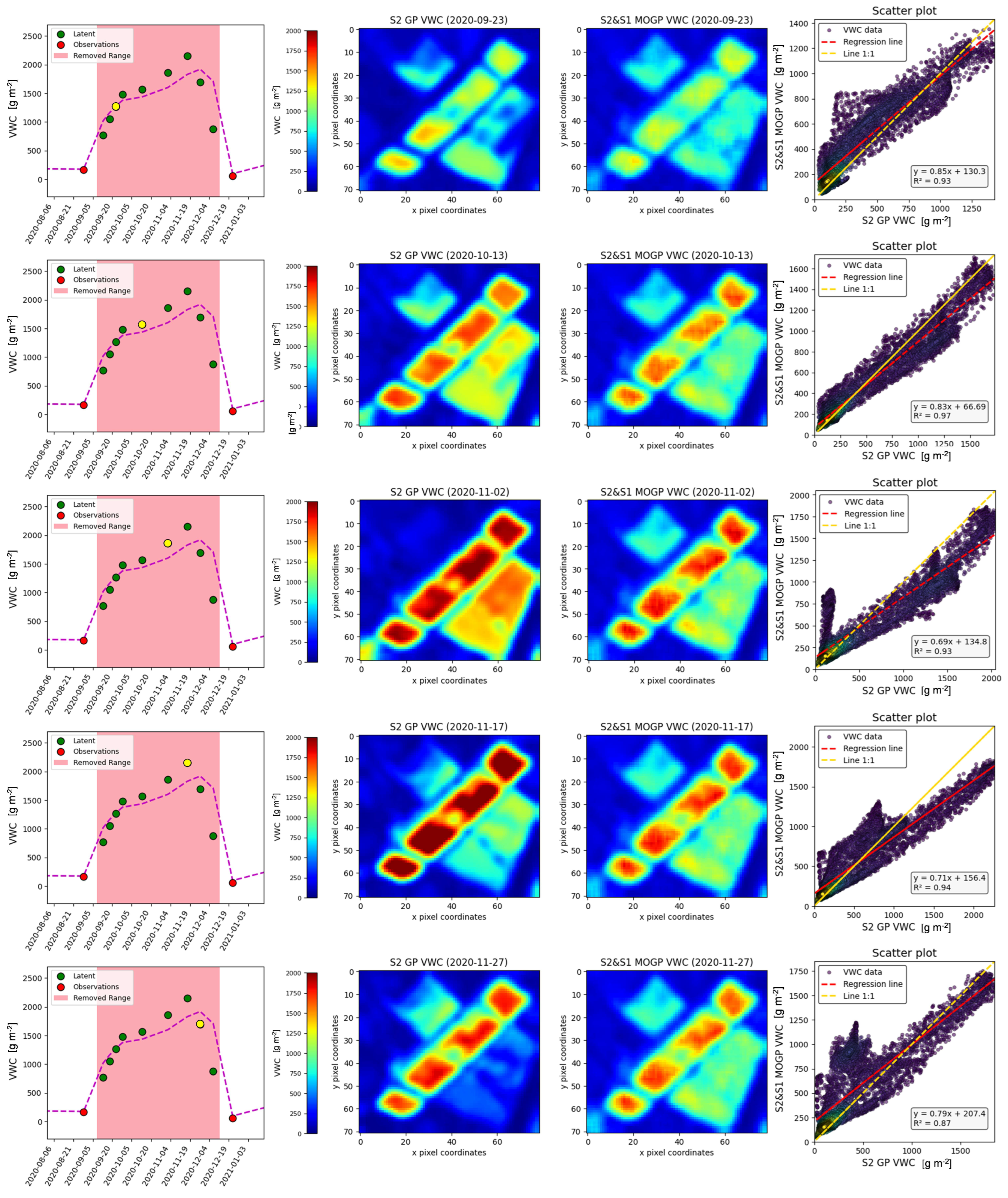
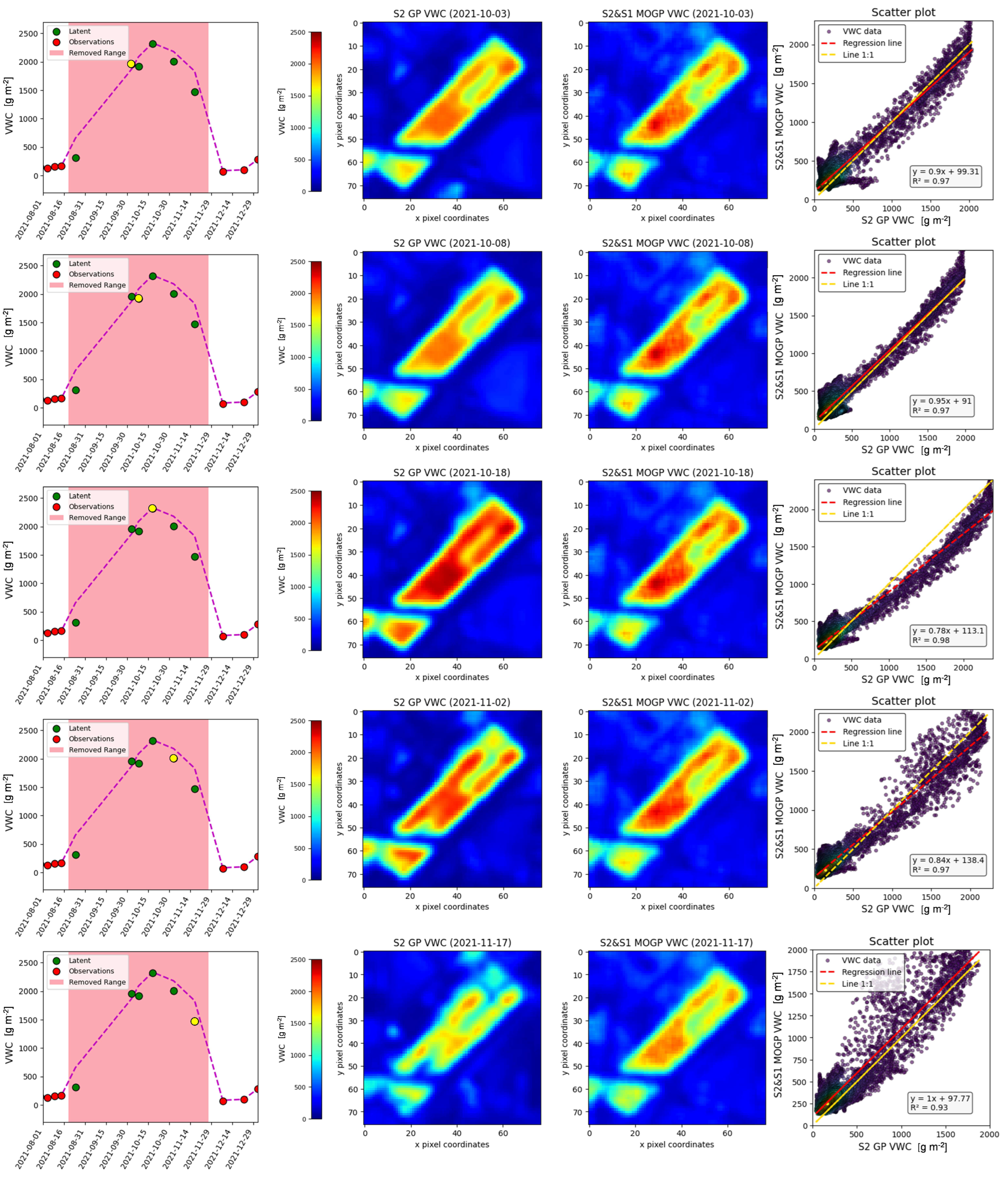
3.3. Spatiotemporal Mapping of Reconstructed VWC Based on S1 & S2 Synergy

The S1 & S2 temporal trends presented in Figure 3 and Figure 4 and the best MOGP model selected in Section 3.2.2 were used to demonstrate the feasibility of VWC maps reconstruction based on the S1 & S2 synergy. To accomplish this, we trained an independent CONV model per pixel over two subsets of the BVCR study site. The first subset (red dotted rectangle in Figure 1) contains three winter wheat paddocks that belong to the 2020 crop campaign and its surface is 56 hectares (71 × 79 pixels at 10 m). The second subset (orange dotted rectangle in Figure 1) consisted of a large homogeneous parcel of winter wheat from the crop campaign 2021 located not far from the first, its size is 58.5 hectares (76 × 77 pixels at 10 m). For each pixel in the S1 & S2 dataset, a CONV model was initialized with the parameters described in Section 2.5 and then trained using 500 iterations. It is worth pointing out that both spatial subsets selected for the application of the MOGP regression, have had the same crop rotation and management according to the agronomic practices of the HAEE. Winter wheat irrigation has been conducted during three distinct vegetative stages along the phenological cycle. While it is true that we applied the CONV model to the whole S1 & S2 dataset for both spatial subsets reconstructing 44 S1 & S2 MOGP VWC maps for the 2020 winter wheat site and 52 for 2021, we focused on the removed ranges to perform a posterior error metrics analysis. The global $R^2$ values for the complete spatiotemporal regression were ${\overline{R^2}}_{subse{t}_1}$ = 0.72 and ${\overline{R^2}}_{subse{t}_2}$ = 0.67 and their related processing time: $t_{subse{t}_1}$ = 70 h and $t_{subse{t}_2}$ = 54 h approximately (processor: 11th Gen Intel(R) Core(TM) i7-1195G7 @ 2.90 GHz 64 bits, RAM: 16 GB). The MOGP technique allowed the reconstruction of each channel in the S1 & S2 dataset independently. It means that, regardless of the acquisition dates of S1 and S2, the CONV model generated a VWC map that coincides with the S2 pass over the study area. Similarly, a reconstructed RVI map was also produced for each S1 acquisition date. The main advantage of MOGP is that there is no need for synchronicity between the acquisitions of S1 and S2. Although the MOGP regression models support the daily temporal resolution (the temporal resolution of each channel can be adjusted independently), we did not modify the S1 and S2 original observation dates. In summary, the temporal resolution of each reconstructed independent channel follows the same pattern as the acquisitions of S1 and S2 over the study area. Consequently, we obtained 44 S1 & S2 MOGP VWC maps for the 2020 wheat campaign and 52 for 2021. Figure 8 show the spatiotemporal reconstruction of VWC maps over the winter wheat paddocks of the BVCR 2020 crop campaign. The vegetation phenology (left) and the scatter plots (right) underpin the S1 & S2 MOGP VWC maps accurately for each assessment date. It is desirable to present the synergy results for the greenness stage of winter wheat at two different locations of the study site. Furthermore, the reconstructed VWC maps for the 2021 winter wheat site are shown in Figure 9. Seeking to prioritize the evaluation of the MOGP within the vegetative development stage of winter wheat plants, we calculated the average $R^2$ values for the scatter plots presented in Figure 8 and Figure 9, we obtained ${\overline{R^2}}_{whea{t}_{2020}}$ = 0.95 and ${\overline{R^2}}_{whea{t}_{2021}}$ = 0.96, which shows the strong correlation of S2 GP VWC and S1 & S2 MOGP VWC maps.

4. Discussion

We explored the feasibility of fusing S1 & S2 data streams with a MOGP approach for cloud-free VWC time series mapping. This study provides a potentially powerful research line that deserves to be carefully analyzed. In the following, time and frequency domain similarities in the S1 & S2 dataset (Section 4.1), MOGP modeling and assessment (Section 4.2), S1 & S2-based spatiotemporal mapping of VWC (Section 4.4), and finally advantages and opportunities for improvement of the fusion approach (Section 4.3) are discussed.

4.1. Time and Frequency Domain Similarities in the S1 & S2 Dataset

GEE proved to be an invaluable tool for processing and downloading Copernicus data quickly, efficiently and accurately. Cloud-processed time series of VWC derived from S2 data produced the typical phenological profile of winter wheat at the study site as was also presented by Caballero et al. [54]. The LAI mapping of winter wheat at the BVCR based on S1 radar data was explored by Caballero et al. [25], demonstrating the efficacy of merging distinct S1 acquisition geometries to retrieve wheat LAI in southern Argentina. In the present study, we analyzed the RVI for two distinct S1 orbits that allow having two radar channels to merge the S1 & S2 time series. Regarding the wheat growth cycle at the focused area, we found the same temporal trends for S1 RVI and S1 LAI GP model developed by Caballero et al. [25]. In Figure 3d and Figure 4d an amplitude offset of RVI for orbit 68 and orbit 141 can be appreciated. These RVI differences, which are related to the mismatch of the local incidence angle, provide valuable information on the three-dimensional structure of the vegetation. The BVCR’s representative crop rotation at the study site was faithfully reproduced by long time series of S2 GP VWC (see Figure 3a and Figure 4a). The S2 GP VWC and S1 RVI time series follow the same temporal patterns, so three phenological cycles (corn-sunflower-wheat) can be captured at the study sites (see Figure 1). In addition, this time correspondence enabled us to gauge the spectral similarities in the S1 & S2 dataset. The frequency domain analysis determines the peak and position of the principal spectral components that are mainly related to crop rotation and phenology. Seeking to customize the response of the SM kernels we selected Q = 4 prioritizing the most representative spectral components in the S1 & S2 dataset (see Section 2.5).

4.2. MOGP Modelling and Assessment

We evaluated several MOGP kernels as well as the SOGP SM approaches aiming to select the best one for the spatiotemporal reconstruction of VWC maps. We presented a set of error metrics in Table 2 and Table 3 for each MOGP kernel, but finally, we adopted the NRMSE for cross-model comparison. The poor capability of SOGP to reconstruct VWC in the absence of optical data can be easily observed for winter wheat ROI-1 and ROI-2. All latent values are remarkably underestimated, therefore, the true VWC profiles are entirely lost (see Figure 5). In the SOGP approach, the spectral mixture kernels are trained independently on each channel, which fails to account for the cross-spectral similarity between S1 & S2 time series. While it is true that other MOGP kernels such as CSM and SM-LMC reached an acceptably high performance for the 2020 winter wheat site, the CONV model was the only one able to tackle the VWC time series reconstruction for both averaged ROIs (see Figure 7). CONV makes use of the convolution theorem to model cross-channel dependencies in the S1 & S2 datasets by means of cross-convolution in the spectral domain. The cross-spectral similarity of the S1 & S2 time series, in this regard (see Section 4.1), is the backbone of the spectral mixture approach (see Figure 6). In terms of S1 & S2 dataset configuration, we assessed two or three-channel fusion models. Regarding the CONV model, superior results were found for both winter wheat averaged ROIs (see Table 2 and Table 3) when the S1 & S2 dataset is fused with S1 RVI orbit 68 instead of S1 RVI orbit 141. We obtained $NRMS{E}_{(S2\&S1,orbit68)}$ = 14.97% and $NRMS{E}_{(S2\&S1,orbit141)}$ = 20.05% for winter wheat 2020 ROI-1 and a two-channel dataset. In the same way, $NRMS{E}_{(S2\&S1,orbit68)}$ = 14.61% and $NRMS{E}_{(S2\&S1,orbit141)}$ = 15.68% for ROI-2. When it comes to three-channel S1 & S2 datasets, the following scenarios were encountered: (i) the accuracy of the CONV kernel increases for ROI-2 (wheat 2021), $NRMS{E}_{(S2\&S1,orbits68\&141)}$ = 10.1% and; (ii) a slight accuracy loss is reflected by the CONV model over the ROI-1 (wheat 2020), $NRMS{E}_{(S2\&S1,orbits68\&141)}$ = 16.1%. These results are directly connected to the fact that the number of S2 cloud-free acquisitions over ROI-1 and ROI-2 is different. Furthermore, they are unevenly spaced, so the S2 GP VWC time series have different frequency spectra in each case.

4.3. S1 & S2-Based Spatiotemporal Mapping of Vegetation Water Content

The outstanding reconstruction results delivered by the CONV model over the two selected subsets of the study site highlight its ability to fuse EO S1 & S2 data for cloud-free crop trait mapping purposes. Thanks to the guidance of the radar data stream, CWV maps were reconstructed by MOGP even in the absence of optical data. Accurate reconstructed VWC maps were obtained for both studied subsets when a CONV model was trained on a per-pixel basis. The land cover spatiotemporal heterogeneity was correctly captured thanks to this strategy. We focused exclusively on the mapping of winter wheat paddocks, nevertheless, other crop types are present in the scenes such as pasture and legumes and even more differ across multiple crop seasons. The CONV model was able to accurately reconstruct the VWC maps over all parcels, regardless of the land cover type (see Figure 8 and Figure 9). It suggests that the MOGP technique can be generically applied, as long as there is sufficiently complementary information present in the radar signal. At the same time, as a Bayesian nonparametric probabilistic ML regression algorithm, MOGP provides an automatic mechanism to construct and calibrate uncertainties. Uncertainty maps offer the opportunity to assess the confidence of predictions and construct reliability maps at pixel level [76].

4.4. Advantages and Opportunities for Improvement of the Fusing Approach

The S1 & S2 time series fusing approach presented here offers attractive and powerful opportunities to be further exploited. Firstly, there is the actual feasibility of successfully implementing cloud-free VWC map reconstruction techniques by taking advantage of the all-weather availability of S1 radar data. Fusing S1 SAR and S2 optical imagery proved particularly useful for monitoring crops’ VWC in southern Argentina, and can be easily extrapolated to high-latitude cloudy regions worldwide. Secondly, MOGP can also be used for gap-filling S2 time series by combining optical data from other EO systems like Landsat-8 or Sentinel-3. Likewise, also other optically-derived variables can be targeted that align well with radar data, such as LAI [29]. Furthermore, thirdly, the ever-increasing supply of emerging radar satellite constellations in different frequency bands poses a revolutionary paradigm [77]. Altogether, the Earth observation scenario for the next few years is extremely promising and requires further exploration of MOGP techniques.

On the downside, it is worth emphasizing that the training time was rather long (see Table 2 and Table 3) when the data from S1 and S2 were combined to reconstruct the VWC maps (see Section 3.3). The long runtime constitutes the main bottleneck of the MOGP technique. Training MOGP algorithms is a challenging task as it involves a large number of hyperparameters to model all the inter-channel cross-correlations in the spectral domain. Some attempts were explored to further improve the results. Seeking to substitute the per-pixel optimization step Belda et al. [37] suggested optimizing a GP for an averaged ROI and then using the hyperparameters of the optimized model. This approach could reduce the long processing time of S1 & S2 datasets but is at a risk to account for the cropland’s spatiotemporal variability. We had tested that approach; however, it appeared that the results in our context were unsatisfactory, and this path was therefore discarded. Follow-up research may attempt to address this limitation. Several alternative mechanisms can be explored to accelerate the training phase of MOGP. They can be divided into two groups: technical and theoretical solutions. Technical solutions include using a more powerful computer (RAM ≥ 64 GB), considering fewer observations for model training, reducing the number of spectral components, or deploying the code in a Graphics Processing Unit (GPU) environment. Theoretical solutions include using a sparse model, e.g., as presented by Titsias [78], or a stochastic gradient descent [79].

5. Conclusions

Cloud-free optical imagery is usually scarce over cloud-prone agroecosystems, implying that crop monitoring is often limited to a few observations during key phenological development stages. The synergy of optical with complementary all-weather SAR data can provide valuable insights into specific agricultural areas, even in the presence of persistent cloud cover. In our study, we demonstrated that fusing time series of S1 SAR and S2 optical data through MOGP proved to be a powerful and innovative methodology to reconstruct cloud-free time series data streams over the entire growing season. Pursuing the development of a powerful fusion approach that learns the dependencies of S1 & S2 time series data, we applied a processing framework for selecting the best MOGP model. The S1 & S2 MOGP CONV model was validated with relatively high accuracy against S2 GP VWC retrieved data over two winter wheat fields belonging to the BVCR 2020 and 2021 crop campaigns (wheat 2020: $NRMS{E}_{(S2\&S1,orbits68\&141)}$ = 16.1% and wheat 2021: $NRMS{E}_{(S2\&S1,orbits68\&141)}$ = 10.1%). The CONV models were afterward applied iteratively at the pixel level to reconstruct removed S2 acquisitions. The reconstructed VWC maps in the absence of optical data showed spatiotemporal consistency and made it possible to accurately capture complete phenology curves. We conclude that the cross-correlation of the time series of S1 and S2 data can be exploited for the purpose of cloud-free large-scale reconstructing of optical-imagery-derived crop trait data streams. Further research must be conducted to deploy the MOGP strategy over other croplands and target other vegetation traits while keeping the runtime within acceptable limits.

References

1. Verrelst, J.; Camps-Valls, G.; Muñoz-Marí, J.; Rivera, J.P.; Veroustraete, F.; Clevers, J.G.P.W.; Moreno, J. Optical remote sensing and the retrieval of terrestrial vegetation bio-geophysical properties—A review. ISPRS J. Photogramm. Remote Sens. 2015, 108, 273–290. [Google Scholar] [CrossRef]
2. Verrelst, J.; Malenovský, Z.; Van der Tol, C.; Camps-Valls, G.; Gastellu-Etchegorry, J.P.; Lewis, P.; North, P.; Moreno, J. Quantifying Vegetation Biophysical Variables from Imaging Spectroscopy Data: A Review on Retrieval Methods. Surv. Geophys. 2019, 40, 589–629. [Google Scholar] [CrossRef] [Green Version]
3. Quemada, C.; Pérez-Escudero, J.M.; Gonzalo, R.; Ederra, I.; Santesteban, L.G.; Torres, N.; Iriarte, J.C. Remote Sensing for Plant Water Content Monitoring: A Review. Remote Sens. 2021, 13, 2088. [Google Scholar] [CrossRef]
4. D’Urso, G.; Richter, K.; Calera, A.; Osann, M.A.; Escadafal, R.; Garatuza-Pajan, J.; Hanich, L.; Perdigão, A.; Tapia, J.B.; Vuolo, F. Earth Observation products for operational irrigation management in the context of the PLEIADeS project. Agric. Water Manag. 2010, 98, 271–282. [Google Scholar] [CrossRef]
5. Clevers, J.G.P.W.; Kooistra, L.; Schaepman, M.E. Estimating canopy water content using hyperspectral remote sensing data. Int. J. Appl. Earth Obs. Geoinf. 2010, 12, 119–125. [Google Scholar] [CrossRef]
6. Wocher, M.; Berger, K.; Danner, M.; Mauser, W.; Hank, T. Physically-based retrieval of canopy equivalent water thickness using hyperspectral data. Remote Sens. 2018, 10, 1924. [Google Scholar] [CrossRef] [Green Version]
7. Gerhards, M.; Schlerf, M.; Mallick, K.; Udelhoven, T. Challenges and Future Perspectives of Multi-/Hyperspectral Thermal Infrared Remote Sensing for Crop Water-Stress Detection: A Review. Remote Sens. 2019, 11, 1240. [Google Scholar] [CrossRef] [Green Version]
8. Bowman, W.D. The relationship between leaf water status, gas exchange, and spectral reflectance in cotton leaves. Remote Sens. Environ. 1989, 30, 249–255. [Google Scholar] [CrossRef]
9. Ustin, S.L.; Riaño, D.; Hunt, E.R. Estimating canopy water content from spectroscopy. Israel J. Plant Sci. 2012, 60, 9–23. [Google Scholar] [CrossRef] [Green Version]
10. Berger, M.; Moreno, J.; Johannessen, J.A.; Levelt, P.F.; Hanssen, R.F. ESA’s sentinel missions in support of Earth system science. Remote Sens. Environ. 2012, 120, 84–90. [Google Scholar] [CrossRef]
11. Drusch, M.; Del Bello, U.; Carlier, S.; Colin, O.; Fernandez, V.; Gascon, F.; Hoersch, B.; Isola, C.; Laberinti, P.; Martimort, P.; et al. Sentinel-2: ESA’s Optical High-Resolution Mission for GMES Operational Services. Remote. Sens. Environ. 2012, 120, 25–36. [Google Scholar] [CrossRef]
12. Amin, E.; Verrelst, J.; Rivera-Caicedo, J.P.; Pipia, L.; Ruiz-Verdú, A.; Moreno, J. Prototyping Sentinel-2 green LAI and brown LAI products for cropland monitoring. Remote Sens. Environ. 2021, 255, 112168. [Google Scholar] [CrossRef]
13. Delloye, C.; Weiss, M.; Defourny, P. Retrieval of the canopy chlorophyll content from Sentinel-2 spectral bands to estimate nitrogen uptake in intensive winter wheat cropping systems. Remote Sens. Environ. 2018, 216, 245–261. [Google Scholar] [CrossRef]
14. Brede, B.; Verrelst, J.; Gastellu-Etchegorry, J.P.; Clevers, J.G.; Goudzwaard, L.; den Ouden, J.; Verbesselt, J.; Herold, M. Assessment of workflow feature selection on forest LAI prediction with sentinel-2A MSI, landsat 7 ETM+ and Landsat 8 OLI. Remote. Sens. 2020, 12, 915. [Google Scholar] [CrossRef] [Green Version]
15. Verrelst, J.; Rivera, J.; Veroustraete, F.; Muñoz Marí, J.; Clevers, J.; Camps-Valls, G.; Moreno, J. Experimental Sentinel-2 LAI estimation using parametric, non-parametric and physical retrieval methods—A comparison. ISPRS J. Photogramm. Remote Sens. 2015, 108, 260–272. [Google Scholar] [CrossRef]
16. Estévez, J.; Salinero-Delgado, M.; Berger, K.; Pipia, L.; Rivera-Caicedo, J.P.; Wocher, M.; Reyes-Muñoz, P.; Tagliabue, G.; Boschetti, M.; Verrelst, J. Gaussian processes retrieval of crop traits in Google Earth Engine based on Sentinel-2 top-of-atmosphere data. Remote. Sens. Environ. 2022, 273, 112958. [Google Scholar] [CrossRef]
17. Torres, R.; Snoeij, P.; Geudtner, D.; Bibby, D.; Davidson, M.; Attema, E.; Potin, P.; Rommen, B.; Floury, N.; Brown, M.; et al. GMES Sentinel-1 mission. Remote Sens. Environ. 2012, 120, 9–24. [Google Scholar] [CrossRef]
18. Ulaby, F.T.; Aslam, A.; Dobson, M.C. Effects of Vegetation Cover on the Radar Sensitivity to Soil Moisture. IEEE Trans. Geosci. Remote Sens. 1982, GE-20, 476–481. [Google Scholar] [CrossRef]
19. Karam, M.A.; Fung, A.K.; Lang, R.H.; Chauhan, N.S. A microwave scattering model for layered vegetation. IEEE Trans. Geosci. Remote Sens. 1992, 30, 767–784. [Google Scholar] [CrossRef] [Green Version]
20. Bousbih, S.; Zribi, M.; Lili-Chabaane, Z.; Baghdadi, N.; El Hajj, M.; Gao, Q.; Mougenot, B. Potential of Sentinel-1 Radar Data for the Assessment of Soil and Cereal Cover Parameters. Sensors 2017, 17, 2617. [Google Scholar] [CrossRef] [Green Version]
21. Rozenstein, O.; Siegal, Z.; Blumberg, D.G.; Adamowski, J. Investigating the backscatter contrast anomaly in synthetic aperture radar (SAR) imagery of the dunes along the Israel–Egypt border. Int. J. Appl. Earth Obs. Geoinf. 2016, 46, 13–21. [Google Scholar] [CrossRef]
22. Gao, S.; Niu, Z.; Huang, N.; Hou, X. Estimating the Leaf Area Index, height and biomass of maize using HJ-1 and RADARSAT-2. Int. J. Appl. Earth Obs. Geoinf. 2013, 24, 1–8. [Google Scholar] [CrossRef]
23. McNairn, H.; Kross, A.; Lapen, D.; Caves, R.; Shang, J. Early season monitoring of corn and soybeans with TerraSAR-X and RADARSAT-2. Int. J. Appl. Earth Obs. Geoinf. 2014, 28, 252–259. [Google Scholar] [CrossRef]
24. Zhang, Y.; Venkatachalam, A.S.; Huston, D.; Xia, T. Advanced signal processing method for ground penetrating radar feature detection and enhancement. In Nondestructive Characterization for Composite Materials, Aerospace Engineering, Civil Infrastructure, and Homeland Security 2014; SPIE: Bellingham, WA, USA, 2014; Volume 9063, pp. 276–289. [Google Scholar] [CrossRef]
25. Caballero, G.; Pezzola, A.; Winschel, C.; Casella, A.; Sanchez Angonova, P.; Orden, L.; Berger, K.; Verrelst, J.; Delegido, J. Quantifying Irrigated Winter Wheat LAI in Argentina Using Multiple Sentinel-1 Incidence Angles. Remote Sens. 2022, 14, 5867. [Google Scholar] [CrossRef] [PubMed]
26. Mattia, F.; Balenzano, A.; Satalino, G.; Lovergine, F.; Peng, J.; Wegmuller, U.; Cartus, O.; Davidson, M.W.J.; Kim, S.; Johnson, J.; et al. Sentinel-1 & Sentinel-2 for SOIL Moisture Retrieval at Field Scale. In Proceedings of the IGARSS 2018–2018 IEEE International Geoscience and Remote Sensing Symposium, IEEE, Valencia, Spain, 22–27 July 2018; pp. 6143–6146. [Google Scholar] [CrossRef]
27. Satalino, G.; Mattia, F.; Balenzano, A.; Lovergine, F.P.; Rinaldi, M.; De Santis, A.P.; Ruggieri, S.; García, D.A.N.; Gómez, V.P.; Ceschia, E.; et al. Sentinel-1 & Sentinel-2 Data for Soil Tillage Change Detection. In Proceedings of the IGARSS 2018–2018 IEEE International Geoscience and Remote Sensing Symposium, IEEE, Valencia, Spain, 22–27 July 2018; pp. 6627–6630. [Google Scholar] [CrossRef]
28. Veloso, A.; Mermoz, S.; Bouvet, A.; Le Toan, T.; Planells, M.; Dejoux, J.F.; Ceschia, E. Understanding the temporal behavior of crops using Sentinel-1 and Sentinel-2-like data for agricultural applications. Remote Sens. Environ. 2017, 199, 415–426. [Google Scholar] [CrossRef]
29. Pipia, L.; Muñoz-Marí, J.; Amin, E.; Belda, S.; Camps-Valls, G.; Verrelst, J. Fusing optical and SAR time series for LAI gap filling with multioutput Gaussian processes. Remote Sens. Environ. 2019, 235, 111452. [Google Scholar] [CrossRef] [PubMed]
30. Druce, D.; Tong, X.; Lei, X.; Guo, T.; Kittel, C.M.M.; Grogan, K.; Tottrup, C. An Optical and SAR Based Fusion Approach for Mapping Surface Water Dynamics over Mainland China. Remote Sens. 2021, 13, 1663. [Google Scholar] [CrossRef]
31. Caballero, G.; Delegido, J.; Verrelst, J. Estimación del LAI de la vegetación a partir de la sinergia Sentinel 1 -Sentinel 2. ResearchGate 2018. [Google Scholar] [CrossRef]
32. Tona, C.; Bua, R. Open Source Data Hub System: Free and open framework to enable cooperation to disseminate Earth Observation data and geo-spatial information. EGU Gen. Assem. Conf. Abstr. 2018, 20, 13038. [Google Scholar]
33. Pipia, L.; Amin, E.; Belda, S.; Salinero-Delgado, M.; Verrelst, J. Green LAI Mapping and Cloud Gap-Filling Using Gaussian Process Regression in Google Earth Engine. Remote. Sens. 2021, 13, 403. [Google Scholar] [CrossRef]
34. Gorelick, N.; Hancher, M.; Dixon, M.; Ilyushchenko, S.; Thau, D.; Moore, R. Google Earth Engine: Planetary-scale geospatial analysis for everyone. Remote Sens. Environ. 2017, 202, 18–27. [Google Scholar] [CrossRef]
35. Kumar, L.; Mutanga, O. Google Earth Engine Applications Since Inception: Usage, Trends, and Potential. Remote Sens. 2018, 10, 1509. [Google Scholar] [CrossRef] [Green Version]
36. Rasmussen, C.E.; Williams, C.K.I. Gaussian Processes for Machine Learning; The MIT Press: New York, NY, USA, 2006. [Google Scholar]
37. Belda, S.; Pipia, L.; Morcillo-Pallarés, P.; Verrelst, J. Optimizing Gaussian Process Regression for Image Time Series Gap-Filling and Crop Monitoring. Agronomy 2020, 10, 618. [Google Scholar] [CrossRef]
38. Bonilla, E.V.; Chai, K.; Williams, C. Multi-task Gaussian Process Prediction. Adv. Neural Inf. Process. Syst. 2007, 20. Available online: https://proceedings.neurips.cc/paper/2007/hash/66368270ffd51418ec58bd793f2d9b1b-Abstract.html (accessed on 21 February 2023).
39. Álvarez, M.A.; Rosasco, L.; Lawrence, N.D. Kernels for Vector-Valued Functions: A Review. MAL 2012, 4, 195–266. [Google Scholar] [CrossRef] [Green Version]
40. Goovaerts, P. Geostatistics for Natural Resources Evaluation; Oxford University Press: Oxford, UK, 1997. [Google Scholar]
41. Lin, Q.; Hu, J.; Zhou, Q.; Cheng, Y.; Hu, Z.; Couckuyt, I.; Dhaene, T. Multi-output Gaussian process prediction for computationally expensive problems with multiple levels of fidelity. Knowl.-Based Syst. 2021, 227, 107151. [Google Scholar] [CrossRef]
42. Alvarez, M.A.; Ward, W.; Guarnizo, C. Non-linear process convolutions for multi-output Gaussian processes. In Proceedings of the 22nd International Conference on Artificial Intelligence and Statistics, Naha, Okinawa, Japan, 16–18 April 2019; pp. 1969–1977. Available online: https://proceedings.mlr.press/v89/alvarez19a.html (accessed on 21 February 2023).
43. de Wolff, T.; Cuevas, A.; Tobar, F. MOGPTK: The Multi-Output Gaussian Process Toolkit. Neurocomputing 2020, 424, 49–53. [Google Scholar] [CrossRef]
44. Kim, Y.; Jackson, T.; Bindlish, R.; Lee, H.; Hong, S. Radar Vegetation Index for Estimating the Vegetation Water Content of Rice and Soybean. IEEE Geosci. Remote Sens. Lett. 2012, 9, 564–568. [Google Scholar]
45. Rasmussen, C.E. Gaussian Processes in Machine Learning. In Advanced Lectures on Machine Learning; Springer: Berlin, Germany, 2004; pp. 63–71. [Google Scholar] [CrossRef] [Green Version]
46. Snee, R.D. Validation of Regression Models: Methods and Examples. Technometrics 1977, 19, 415–428. [Google Scholar] [CrossRef]
47. Love, B.C.; Jones, M. Bayesian Learning. In Encyclopedia of the Sciences of Learning; Springer: Boston, MA, USA, 2012; pp. 415–417. [Google Scholar] [CrossRef]
48. Wackernagel, H. Multivariate Geostatistics: An Introduction with Applications; Springer: Berlin, Germany, 2013. [Google Scholar]
49. Barry, R.P.; Hoef, J.M.V. Blackbox Kriging: Spatial Prediction without Specifying Variogram Models on JSTOR. J. Agric. Biol. Environ. Stat. 1996, 1, 297–322. [Google Scholar] [CrossRef]
50. Ver Hoef, J.M.; Barry, R.P. Constructing and fitting models for cokriging and multivariable spatial prediction. J. Stat. Plan. Inference 1998, 69, 275–294. [Google Scholar] [CrossRef]
51. Higdon, D. Space and Space-Time Modeling using Process Convolutions. In Quantitative Methods for Current Environmental Issues; Springer: London, UK, 2002; pp. 37–56. [Google Scholar] [CrossRef]
52. Casella, A.; Orden, L.; Pezzola, N.A.; Bellaccomo, C.; Winschel, C.I.; Caballero, G.R.; Delegido, J.; Gracia, L.M.N.; Verrelst, J. Analysis of Biophysical Variables in an Onion Crop (Allium cepa L.) with Nitrogen Fertilization by Sentinel-2 Observations. Agronomy 2022, 12, 1884. [Google Scholar] [CrossRef]
53. Caballero, G.R.; Platzeck, G.; Pezzola, A.; Casella, A.; Winschel, C.; Silva, S.S.; Ludueña, E.; Pasqualotto, N.; Delegido, J. Assessment of Multi-Date Sentinel-1 Polarizations and GLCM Texture Features Capacity for Onion and Sunflower Classification in an Irrigated Valley: An Object Level Approach. Agronomy 2020, 10, 845. [Google Scholar] [CrossRef]
54. Caballero, G.; Pezzola, A.; Winschel, C.; Casella, A.; Sanchez Angonova, P.; Rivera-Caicedo, J.P.; Berger, K.; Verrelst, J.; Delegido, J. Seasonal Mapping of Irrigated Winter Wheat Traits in Argentina with a Hybrid Retrieval Workflow Using Sentinel-2 Imagery. Remote Sens. 2022, 14, 4531. [Google Scholar] [CrossRef]
55. Berger, K.; Rivera Caicedo, J.P.; Martino, L.; Wocher, M.; Hank, T.; Verrelst, J. A Survey of Active Learning for Quantifying Vegetation Traits from Terrestrial Earth Observation Data. Remote. Sens. 2021, 13, 287. [Google Scholar] [CrossRef]
56. Settles, B. Active Learning Literature Survey. University of Wisconsin–Madison, Department of Computer Sciences. 2009. Available online: https://minds.wisconsin.edu/handle/1793/60660 (accessed on 21 February 2023).
57. Salinero-Delgado, M.; Estévez, J.; Pipia, L.; Belda, S.; Berger, K.; Paredes Gómez, V.; Verrelst, J. Monitoring Cropland Phenology on Google Earth Engine Using Gaussian Process Regression. Remote Sens. 2021, 14, 146. [Google Scholar] [CrossRef]
58. Reyes-Muñoz, P.; Pipia, L.; Salinero-Delgado, M.; Belda, S.; Berger, K.; Estévez, J.; Morata, M.; Rivera-Caicedo, J.P.; Verrelst, J. Quantifying Fundamental Vegetation Traits over Europe Using the Sentinel-3 OLCI Catalogue in Google Earth Engine. Remote Sens. 2022, 14, 1347. [Google Scholar] [CrossRef] [PubMed]
59. Verrelst, J.; Rivera-Caicedo, J.P.; Reyes-Muñoz, P.; Morata, M.; Amin, E.; Tagliabue, G.; Panigada, C.; Hank, T.; Berger, K. Mapping landscape canopy nitrogen content from space using PRISMA data. ISPRS J. Photogramm. Remote. Sens. 2021, 178, 382–395. [Google Scholar] [CrossRef]
60. Gutman, G.; Ignatov, A. The derivation of the green vegetation fraction from NOAA/AVHRR data for use in numerical weather prediction models. Int. J. Remote Sens. 1998, 19, 1533–1543. [Google Scholar] [CrossRef]
61. Gitelson, A.; Zur, Y.; Chivkunova, O.; Merzlyak, M. Assessing carotenoid content in plant leaves with reflectance spectroscopy. Photochem. Photobiol. 2002, 75, 272–281. [Google Scholar] [CrossRef]
62. Jia, K.; Liang, S.; Gu, X.; Baret, F.; Wei, X.; Wang, X.; Yao, Y.; Yang, L.; Li, Y. Fractional vegetation cover estimation algorithm for Chinese GF-1 wide field view data. Remote Sens. Environ. 2016, 177, 184–191. [Google Scholar] [CrossRef]
63. Song, W.; Mu, X.; Ruan, G.; Gao, Z.; Li, L.; Yan, G. Estimating fractional vegetation cover and the vegetation index of bare soil and highly dense vegetation with a physically based method. Int. J. Appl. Earth Obs. Geoinf. 2017, 58, 168–176. [Google Scholar] [CrossRef]
64. García-Haro, F.J.; Campos-Taberner, M.; Munoz-Mari, J.; Laparra, V.; Camacho, F.; Sanchez-Zapero, J.; Camps-Valls, G. Derivation of global vegetation biophysical parameters from EUMETSAT Polar System. ISPRS J. Photogramm. Remote. Sens. 2018, 139, 57–74. [Google Scholar] [CrossRef]
65. Lee, J.S.; Jurkevich, L.; Dewaele, P.; Wambacq, P.; Oosterlinck, A. Speckle filtering of synthetic aperture radar images: A review. Remote. Sens. Rev. 1994, 8, 313–340. [Google Scholar] [CrossRef]
66. Lee, J.S. Refined filtering of image noise using local statistics. Comput. Graph. Image Process. 1981, 15, 380–389. [Google Scholar] [CrossRef]
67. Pan, Z.; Hu, Y.; Cao, B. Construction of smooth daily remote sensing time series data: A higher spatiotemporal resolution perspective. Open Geospat. Data Softw. Stand. 2017, 2, 1–11. [Google Scholar] [CrossRef] [Green Version]
68. Savitzky, A.; Golay, M.J.E. Smoothing and Differentiation of Data by Simplified Least Squares Procedures. Anal. Chem. 1964, 36, 1627–1639. [Google Scholar] [CrossRef]
69. Neeff, T.; Dutra, L.V.; Dos Santos, J.R.; Freitas, C.C.; Araujo, L.S. Power spectrum analysis of SAR data for spatial forest characterization in Amazonia. Int. J. Remote Sens. 2005, 26, 2851–2864. [Google Scholar] [CrossRef]
70. Parra, G.; Tobar, F. Spectral Mixture Kernels for Multi-Output Gaussian Processes. Adv. Neural Inf. Process. Syst. 2017, 30. [Google Scholar] [CrossRef]
71. Ulrich, K.R.; Carlson, D.E.; Dzirasa, K.; Carin, L. GP Kernels for Cross-Spectrum Analysis. Adv. Neural Inf. Process. Syst. 2015, 28. Available online: https://proceedings.neurips.cc/paper/2015/hash/285ab9448d2751ee57ece7f762c39095-Abstract.html (accessed on 21 February 2023).
72. Alvarez, M.; Lawrence, N. Sparse Convolved Gaussian Processes for Multi-output Regression. Adv. Neural Inf. Process. Syst. 2008, 21. Available online: https://proceedings.neurips.cc/paper/2008/hash/149e9677a5989fd342ae44213df68868-Abstract.html (accessed on 21 February 2023).
73. van der Wilk, M.; Rasmussen, C.E.; Hensman, J. Convolutional Gaussian Processes. 2017. Available online: https://doi.org/10.48550/ARXIV.1709.01894 (accessed on 21 February 2023).
74. Kingma, D.P.; Ba, J. Adam: A Method for Stochastic Optimization. arXiv 2014. [Google Scholar] [CrossRef]
75. Tobar, F. Bayesian Nonparametric Spectral Estimation. Adv. Neural Inf. Process. Syst. 2018, 31. Available online: https://proceedings.neurips.cc/paper/2018/hash/abd1c782880cc59759f4112fda0b8f98-Abstract.html (accessed on 21 February 2023).
76. Verrelst, J.; Rivera, J.; Moreno, J.; Camps-Valls, G. Gaussian processes uncertainty estimates in experimental Sentinel-2 LAI and leaf chlorophyll content retrieval. ISPRS J. Photogramm. Remote Sens. 2013, 86, 157–167. [Google Scholar] [CrossRef]
77. Paek, S.W.; Balasubramanian, S.; Kim, S.; de Weck, O. Small-Satellite Synthetic Aperture Radar for Continuous Global Biospheric Monitoring: A Review. Remote Sens. 2020, 12, 2546. [Google Scholar] [CrossRef]
78. Titsias, M.K. Variational Model Selection for Sparse Gaussian Process Regression; University of Manchester: Manchester, UK, 2008. [Google Scholar]
79. Kiefer, J.; Wolfowitz, J. Stochastic Estimation of the Maximum of a Regression Function. Ann. Math. Stat. 1952, 23, 462–466. [Google Scholar] [CrossRef]
Figure 1. Overview of BVCR test sites (ROI) for the winter wheat campaigns of the years 2020 and 2021. The red and orange dotted rectangles delimit the MOGP subsets analyzed in Section 3.3. Reference system: WGS84 (EPSG 4326). (For interpretation of the references to color in this figure legend, the reader is referred to the Web version of this article).
Remotesensing 15 01822 g001
Figure 2. Illustration of the processing workflow to obtain maps of vegetation water content over irrigated winter wheat, as described in Section 2.7. The ordinal numbers in the graph refer to the workflow processing steps. The maps show the output obtained by our MOGP VWC models over the BVCR study site in Argentina.
Remotesensing 15 01822 g002
Figure 3. Temporal profiles (mean value and standard deviation) of averaged selected ROI-1 over a winter wheat parcel belonging to the BVCR 2020 crop campaign. S2 GP VWC time series from December 2018 to the end of January 2021 (a). S1 RVI orbit 141 smoothed (dashed blue line) and original (dashed black line) time series (b). S1 RVI orbit 68 smoothed (dashed red line) and original (dashed black line) time series (c). S1 RVI Orbit 68 (red line) and S1 orbit 141 (blue line) RVI time series (d).
Remotesensing 15 01822 g003
Figure 4. Temporal profiles (mean value and standard deviation) of averaged selected ROI-2 over a winter wheat parcel belonging to the BVCR 2021 crop campaign. S2 GP VWC time series from October 2019 to the end of January 2022 (a). S1 RVI orbit 141 smoothed (dashed blue line) and original (dashed black line) time series (b). S1 RVI orbit 68 smoothed (dashed red line) and original (dashed black line) time series (c). S1 RVI Orbit 68 (red line) and S1 orbit 141 (blue line) RVI time series (d).
Remotesensing 15 01822 g004
Figure 5. Performance of the SOGP and MOGP models predictions for VWC data reconstruction based on the S1 & S2 synergy. The green dots represent the latent S2 GP VWC data used to compute the error metrics whereas the red dots correspond to the S2 GP VWC cloud-free observations utilized to train the regression models. The red-shaded area represents the artificially created S2 data gap. SOGP and MOGP predictions performance for the selected winter wheat ROI-1 of the year 2020 (a) and 2021 (b).
Remotesensing 15 01822 g005
Figure 6. Cross-correlation matrix of the S1 & dataset among the channels of the trained MOGP models. The elements of the matrix’s diagonal show the auto-correlations of each channel in the dataset. MOSM model for wheat 2020 (a). CSM model for wheat 2020 (b). SM-LMC model for wheat 2020 (c). CONV model for wheat 2020 (d). MOSM model for wheat 2021 (e). CSM model for wheat 2021 (f). SM-LMC model for wheat 2021 (g). CONV model for wheat 2021 (h).
Remotesensing 15 01822 g006aRemotesensing 15 01822 g006b
Figure 7. CONV posterior predicted mean for a three-channel model. Red dots indicate the original observations for S2 GP VWC (CH-1), S1 RVI orbit 68 (CH-2), and S1 RVI orbit 141 (CH-3) while the green ones are the latent samples. Winter wheat 2020 ROI-1 (a). Winter wheat 2020 ROI-2 (b).
Remotesensing 15 01822 g007
Figure 8. Comparison of S2 GP VWC (original) and S1 & S2 MOGP VWC (reconstructed) maps over a selected subset of the study site (red-dashed rectangle in Figure 1) corresponding to the artificially removed dates: 2020/9/23, 2020/10/13, 2020/11/2, 2020/11/17, and 2020/11/27 of the winter wheat 2020 phenological cycle. For each assessment date, the position of the extracted samples on the phenological curve (yellow dot), the S2 GP VWC map, the reconstructed S1 & S2 MOGP VWC map and the scatterplot between the original and reconstructed VWC maps are shown.
Remotesensing 15 01822 g008
Figure 9. Comparison of S2 GP VWC (original) and S1 & S2 MOGP VWC (reconstructed) maps over a selected subset of the study site (orange-dashed rectangle in Figure 1) corresponding to the artificially removed dates: 2021/10/3, 2021/10/8, 2021/10/18, 2021/11/2, and 2021/11/17 of the winter wheat 2021 phenological cycle. For each assessment date, the position of the extracted samples on the phenological curve (yellow dot), the S2 GP VWC map, the reconstructed S1 & S2 MOGP VWC map and the scatterplot between the original and reconstructed VWC maps are shown.
Remotesensing 15 01822 g009