Article

A New Method for Hour-by-Hour Bias Adjustment of Satellite Precipitation Estimates over Mainland China

1
State Key Laboratory of Hydrology-Water Resources and Hydraulic Engineering, Hohai University, Nanjing 210098, China
2
School of Hydrology and Water Resources, Hohai University, Nanjing 210098, China
3
College of Civil Engineering, Nanjing Forestry University, Nanjing 210037, China
*
Author to whom correspondence should be addressed.
Remote Sens. 2023, 15(7), 1819; https://doi.org/10.3390/rs15071819
Submission received: 28 February 2023 / Revised: 24 March 2023 / Accepted: 27 March 2023 / Published: 29 March 2023
(This article belongs to the Section Remote Sensing in Geology, Geomorphology and Hydrology)

Abstract

:
Highly accurate near-real-time satellite precipitation estimates (SPEs) are important for hydrological forecasting and disaster warning. The near-real quantitative precipitation estimates (REGC) of the recently developed Chinese geostationary meteorological satellite Fengyun 4A (FY4A) have the advantage of high spatial and temporal resolution, but there are errors and uncertainties to some extent. In this paper, a self-adaptive ill-posed least squares scheme based on sequential processing (SISP) is proposed and practiced in mainland China to correct the real-time biases of REGC hour by hour. Specifically, the scheme adaptively acquires sample data by setting temporal and spatial windows and constructs an error-correction model based on the ill-posed least squares method from the perspectives of climate regions, topography, and rainfall intensity. The model adopts the sequential idea to update satellite precipitation data within time windows on an hour-by-hour basis and can correct the biases of real-time satellite precipitation data using dynamically changing parameters, fully taking into account the influence of precipitation spatial and temporal variability. Only short-term historical data are needed to accurately rate the parameters. The results show that the SISP algorithm can significantly reduce the biases of the original REGC, in which the values of relative bias (RB) in mainland China are reduced from 11.2% to 3.3%, and the values of root mean square error (RMSE) are also reduced by about 17%. The SISP algorithm has a better correction in humid and semi-humid regions than in arid and semi-arid regions and is effective in reducing the negative biases of precipitation in each climate region. In terms of rain intensity, the SISP algorithm can improve the overestimation of satellite precipitation estimates for low rain intensity (0.2–1 mm/h), but the correction for high rain intensity (>1 mm/h) needs further improvement. The error component analysis shows that the SISP algorithm can effectively correct the hit bias. This study serves as a valuable reference for real-time bias correction using short-term accumulated precipitation data.

1. Introduction

Precipitation plays a key role in the global water and energy cycle [1]. Its uneven spatial and temporal variability can have a large impact on the water cycle [2,3], which is highly susceptible to natural disasters such as floods, landslides, and droughts [4] and constrains human productive activities [5]. Therefore, timely and accurate precipitation information is important for applications such as weather hazards warning, hydrological simulations, and water resource management [6,7]. Conventional precipitation measurements rely on ground-based rain gauges and radar [8], which are considered to be the most accurate means of precipitation observation, where rain gauge data are generally taken as the “true value of precipitation” [9]. Nevertheless, such methods are easily limited by topography, resulting in uneven distribution of stations and radars, which makes it difficult to access precipitation information with high spatial coherence [2,10]. As remote sensing technology grows by leaps and bounds, a new precipitation measurement method based on the retrieval of satellite remote sensing has come into being [11,12]. This method has become a complement to conventional rain gauges and radar because it can produce continuous precipitation information with wide spatial coverage and temporal continuity and is free from the constraints of topography and vegetation [13,14].
Despite these advantages, real-time pure satellite precipitation estimates (SPEs) contain large errors and uncertainties, such as IMERG-Early, PERSIANN-CCS, etc. [15,16]. This is mainly due to the fact that the retrieval information from satellite sensors is indirect in nature [17] and is vulnerable to sampling errors, sensor limitations, and the estimation process of the retrieval algorithm [18]. Some other high-accuracy satellite precipitation products (e.g., IMERG-Final, GSMaP-Gauge) [19,20] have been produced by merging ground station data or reanalysis precipitation data, but these products cannot support applications related to the emphasis on quasi-real time due to the long time lag and the inability to obtain them on time.
Therefore, many researchers [6,21,22,23,24] have focused on reducing the source-set biases of pure SPEs through real-time error-correction algorithms so that the corrected SPEs can meet the requirements of real-time hydrological applications in terms of both accuracy and timeliness. In particular, a common approach is to calibrate future real-time satellite estimates by establishing a statistical relationship between historical gauge measurements and historical satellite precipitation data [25,26,27,28,29,30,31]. Tian et al. [25] revised TMPA-RT and CMORPH in real time by establishing a statistical relationship between SPEs and station measurements through a Bayesian algorithm. Deng et al. [26] constructed a nonlinear fitting method to correct the bias of GSMaP-Gauge based on the relationship between mean error and precipitation intensity in the Han River basin in China, and the results demonstrated that the method could significantly reduce the random error. Based on a similarity matrix using mean bias removal and multiplicative ratio techniques, Choubin et al. [27] corrected TMPA 3B42 precipitation data on a daily scale by incorporating influence factors (elevation, periodicity, and precipitation), and the results showed that the proposed method can be useful to remove the significant portion of the bias for daily TMPA data. Sun et al. [28] calibrated the IMERG rainfall biases based on the cumulative probability density function (CDF) and found that the method was the most effective in calibrating rainfall from 0 to 100 mm on the monthly scale. Yang et al. [29] incorporated the quantile mapping method (QM) and Gaussian weighted interpolation (GW) to revise the biases of SPEs in real time. Shen et al. [30] proposed an improved CDF method with an adaptive sliding window-based CDF to adjust the bias, and the results showed that the method has robust performance in western China. Chen et al. [31] found that the ill-posed least squares (ILS) method based on the key four elements is better applied in reducing the bias of near-real-time GSMaP-NRT.
However, these calibration schemes suffer from different defects: (1) The more the amount of historical precipitation data (4 to 6 years) used in the above methods, the higher the accuracy of the calibration parameters for the rate determination [25]. Therefore, it is not conducive to the effective calibration of biases by these methods when the lack of historical station data or the shortage of emerging satellite precipitation data makes it challenging to obtain rich historical data. (2) The original ILS algorithm will apply unique and fixed parameters to correct future SPEs once the spatial extent and the number of samples in the training period have been determined. However, as climate warming leads to the increased spatial and temporal heterogeneity of precipitation and the increased frequency of extreme precipitation occurrences [32,33], which will change the error characteristics of precipitation to a certain extent [29], then using only fixed parameters to correct real-time SPEs will bring large uncertainties.
Therefore, building on the previous analyses, a new real-time correction scheme is proposed in this paper, which can accurately correct the real-time satellite precipitation estimates with shorter accumulated historical precipitation data. The new scheme is composed of a self-adaptive ILS algorithm and adopts the principle of sequential processing (SISP) to correct hourly satellite precipitation data: Firstly, the time window is set to obtain short-term accumulated historical data, and then the spatial window of dynamic search is set to adjust the window size adaptively according to the location of regional grid, season, and the characteristics of precipitation. Through this step, valid sample data can be obtained, and the influence of spatial and temporal heterogeneity of precipitation can be minimized. Secondly, the valid sample data and the key influencing factors (topography, climate zone, and rainfall intensity) affecting the precipitation error are incorporated into the ill-posed least squares algorithm together to build the bias-adjustment model. Finally, the corrected precipitation estimate is substituted for the original data using sequential processing to update the time window, improving the quality of the sample data while improving the accuracy of the correction parameters.
Fengyun 4A (FY4A) is a new generation of geostationary meteorological satellites developed in China. Its near-real quantitative precipitation estimation products are characterized by high spatial and temporal resolution, which are beneficial to the forecasting and monitoring of catastrophic weather [34,35], but there are significant errors and uncertainties in the data [36,37]. With the increasing influence of FY series satellite products, it is necessary to adjust the error of their precipitation estimates to meet the requirements of real-time hydrological applications. Therefore, in this paper, the Chinese regional quantitative precipitation estimation (REGC) of FY4A is selected as the study area for hourly revision. The satellite precipitation data and the ground station data used in this study are described in Section 2. The hourly revision method is detailed in Section 3. The performance of the satellite precipitation estimates before and after correction by the algorithm, as well as the improvement of the algorithm in terms of the error components, are presented in Section 4, followed by a discussion and conclusions in Section 5 and Section 6, respectively.

2. Study Area and Data
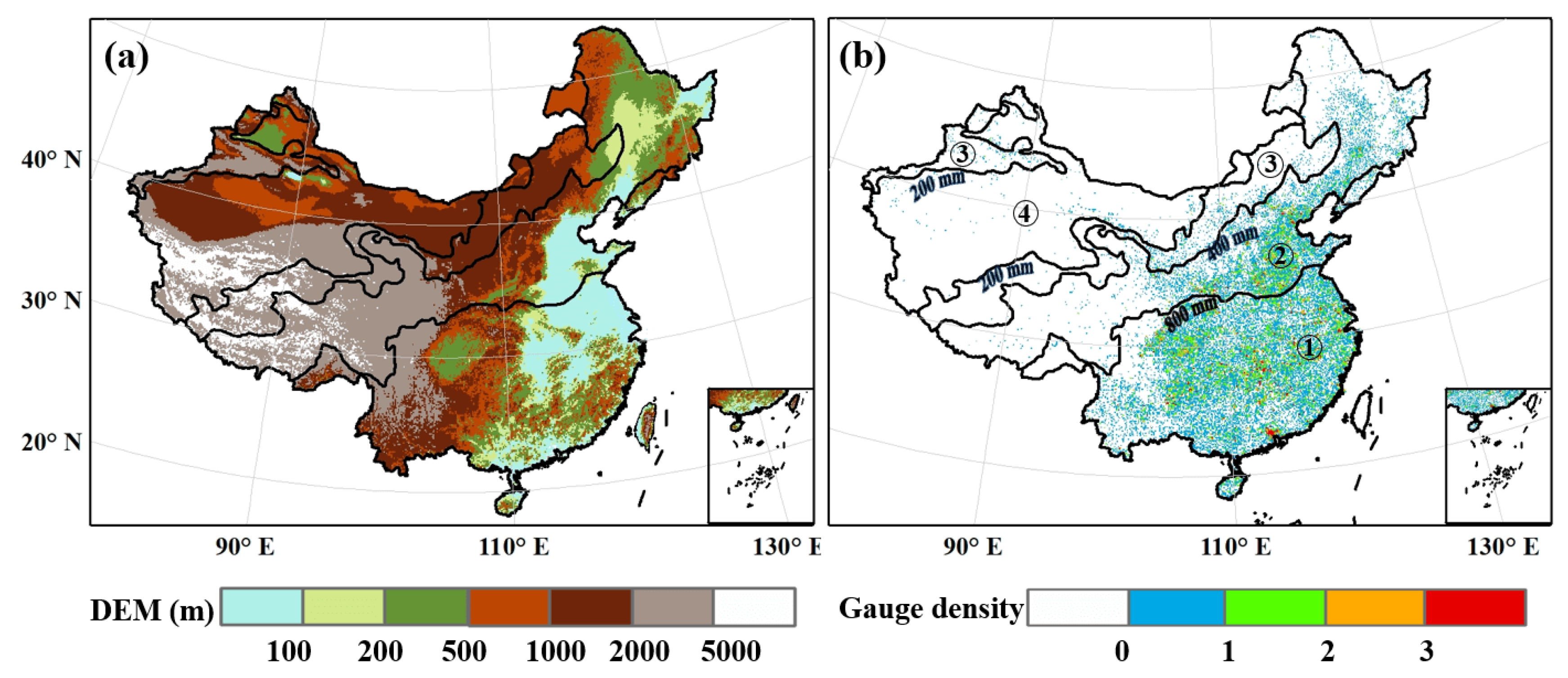
2.1. Study Area

In this paper, Mainland China is taken as the study area, which is located in the southeastern part of Eurasia and adjacent to the western part of the Pacific Ocean (73.5°–135°E, 4°–53.5°N). The Chinese continent is a vast area with a complex topography and diverse climate types. Figure 1a shows the elevation distribution of China, with the terrain being higher in the west and lower in the east.
Under the influence of subtropical high pressure in the western Pacific Ocean and complex topography [38,39], precipitation has obvious spatial and temporal variability, and annual precipitation shows a gradual decrease from the southeast coast to the northwest inland areas [40]. Thus, this paper divides the Chinese continent into four climatic regions based on annual precipitation, as shown in Figure 1b: ① humid region (average annual precipitation > 800 mm) ② semi-humid region (average annual precipitation of 400–800 mm) ③ semi-arid region (average annual precipitation of 200–400 mm) ④ arid region (average annual precipitation < 200 mm). In addition, Figure 1b shows the distribution of the rain gauge stations in each 0.1° × 0.1° grid.

2.2. Study Data

2.2.1. Ground Reference

The ground reference data in this paper is an hourly precipitation grid data set that was obtained by fusing more than 30,000 Chinese automatic stations with the Climate Prediction Center Morphing (CMORPH) at 0.1° × 0.1° scale, which was developed by the National Meteorological Information Center (NMIC) of the China Meteorological Administration and named China Merged Precipitation Analysis (CMPA) [41]. Its distribution in China is characterized by density in the southeast and sparsity in the west (e.g., Figure 1b). The CMPA dataset was produced by fusing observed data with CMORPH data using a two-step fusion method of probability density function (PDF) and optimal interpolation (OI) [42,43]. The accuracy of this dataset is better than its international counterparts, especially for gridded areas containing automatic weather stations, and it can portray the characteristics of hourly precipitation over time to the maximum extent [44,45], making it suitable as ground reference precipitation data for satellite accuracy assessment.

2.2.2. Fengyun 4A

FY4A is the first satellite of the second generation of Chinese geostationary meteorological satellites in the FY-4 series, and its successful launch represents a new era of a new generation of Chinese geostationary meteorological satellites [46]. It carries the Advanced Geostationary Radiation Imager (AGRI), which is an advanced multi-channel scanning radiometer with different observation modes. AGRI observation modes are determined by the temporal resolution of the observations, and the observations are made in 15-min intervals and are positioned and calibrated in the observation gap. There are two scanning modes: the first one is the full disc conventional imaging covering the Asia-Pacific region. In addition to making a full disk observation every hour from the hour to 15 min after the hour, AGRI also takes the first 15 min and the last 15 min of the eight hours of 00:00/03:00/06:00/09:00/12:00/15:00/18:00/21:00 (UTC) as the observation starting time to make a full disk observation, which is three consecutive full disk observations every three hours. Finally, full disk precipitation estimates (DISK) at 4 km/1 h/3 h/6 h/24 h are produced. The second mode is regional conventional imaging, covering 3°–55°N and 60°–137°E. The Chinese regional observation is carried out only at 5 min intervals when there is no full disk observation, and three Chinese regional cloud maps can be obtained by continuous observation for 15 min, which finally produces a real-time precipitation estimate (REGC) at 4 km/5 min.
The precipitation estimate of REGC is selected for this paper due to its higher temporal frequency, wider temporal coverage within the hourly scale, and higher real-time availability than DISK. REGC is a pure satellite precipitation product, which has been downloadable from the official website since 12 March 2018 (http://satellite.nsmc.org.cn/portalsite/default.aspx, accessed on 15 July 2022).

3. Methodology

3.1. Data Pre-Processing

The ground reference data set is at 0.1°/1 h scale, while REGC is at 4 km/5 min scale, so it is unified to the resolution of 0.1°/1 h in this paper. For the temporal scale, the 5 min files of multiple times within 1 h were averaged to obtain the “1 h average precipitation” product, which was described in Zhong et al. [47].

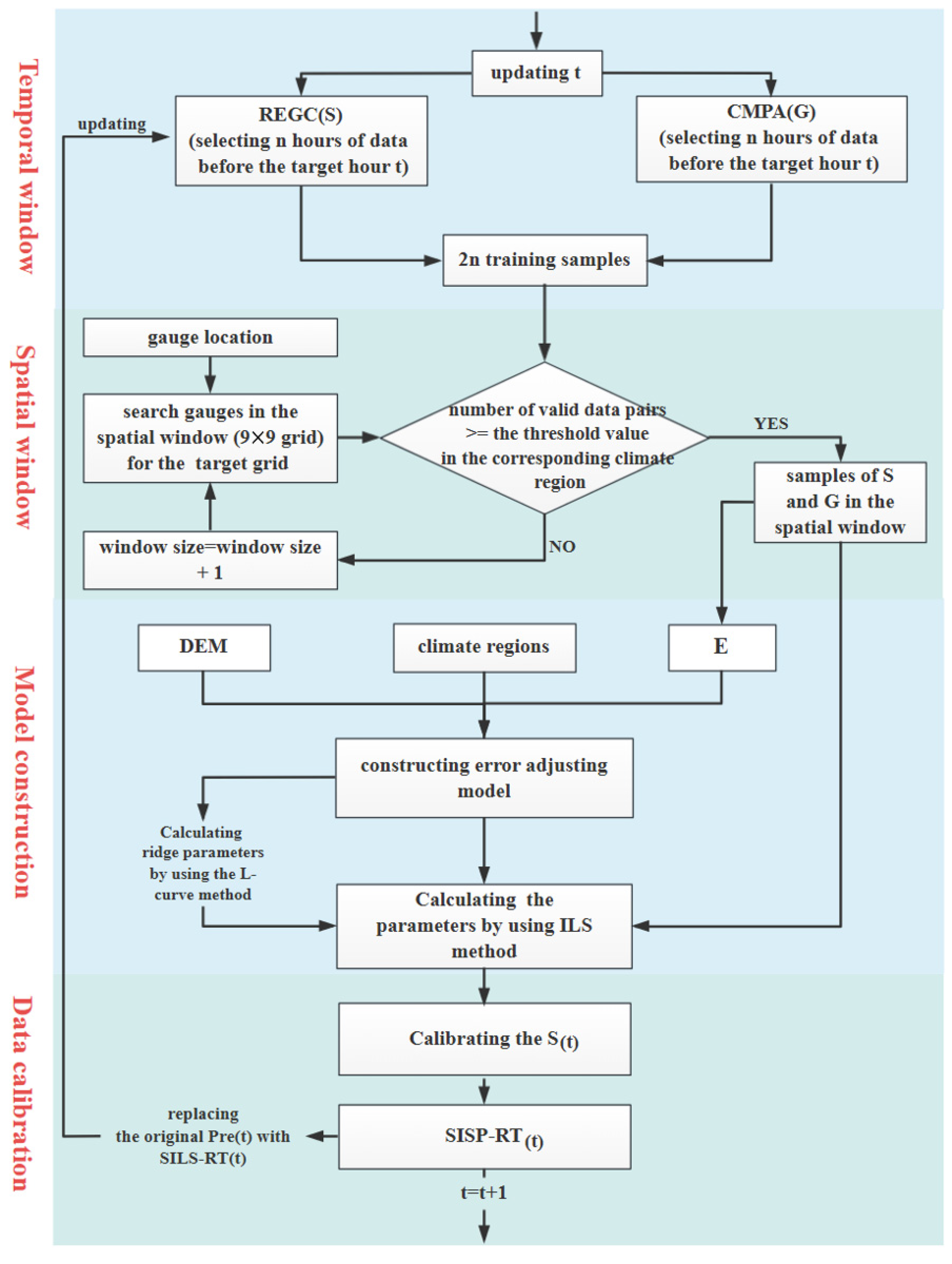
3.2. Bias-Adjusting Procedure

In this paper, a correction scheme of self-adaptive ILS based on sequential process (SISP) is proposed, which can cope with the increasingly complex spatial and temporal variability of precipitation by setting a spatial and temporal window to dynamically acquire training sample data and performing precipitation bias correction on a time-by-time and grid-by-grid basis. Taking the t-th hour precipitation data S t of the original REGC in a region as an example, the revised SISP model is constructed grid by grid, and then the revised real-time satellite precipitation data are named S I S P R T t . The flow chart is shown in Figure 2. The detailed steps are as follows.
(1)
Self-adaptive selection of sample data
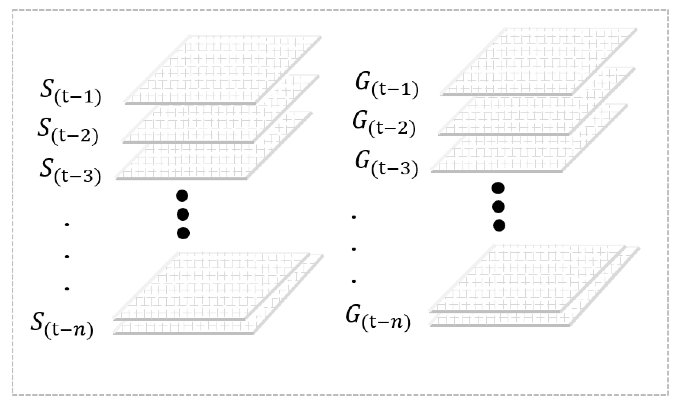
  • Determining the temporal window
Take n hours (excluding the current hour) backward from the current hour t as the time window, which means n historical satellite precipitation data ( S ) and n historical ground station data ( G ) are selected as training sample files, respectively. These files are composed as in Figure 3.
S = S t 1 , S t 2 , , S t j , , S t n  
G = G t 1 , G t 2 , , G t j , , G t n  
The data in S and G in Equations (1) and (2) are required to coincide with each other in time order. If S t j or G t j is not available, both the satellite and ground precipitation data at that time are discarded. Then, continue to select historical data backward, and finally, the number of training samples of both S and G should be ensured to be S .
Since satellite precipitation errors are feature by monthly and daily variations [43], the size of the time window needs to be determined according to the time scale of the precipitation data, and the month (or season) to which the data belongs. The precipitation data used in this paper is at an hourly scale in summer, so 120 h backward from the current hour is taken as the time window.
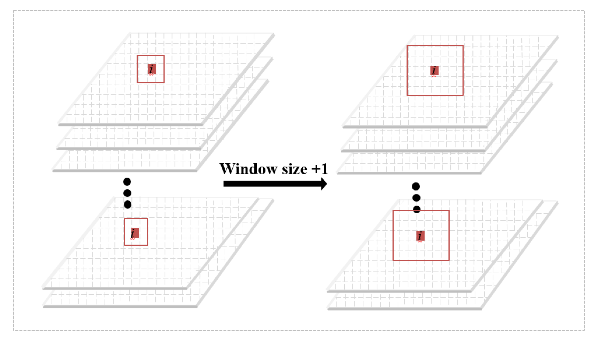
  • Determining the spatial window
Since the spatial resolution of both REGC and CMPA is uniformly 0.1° × 0.1°, and the spatial variability scale of precipitation is around the order of 100 km (approximately 1° × 1°) [48], the initial size of 1° × 1° is chosen as the search range in this paper to be closer to the range of precipitation occurrence. In other words, a spatial window of 9 × 9 grids is set up with the grid i as the center, and it is required that at least one station exists within this spatial window to be used as the valid window to ensure the availability of ground reference stations. In addition, the precipitation intensity of satellite precipitation and ground precipitation in the window is required to be greater than the threshold of 0.1 mm/h to be used as an effective training sample, which is consistent with the threshold suggested in most studies for determining the occurrence/absence of rainfall [49]. This is due to the higher probability of zero precipitation occurrence on the hourly scale and the fact that satellite precipitation and ground precipitation data are prone to large errors in light precipitation events [43]. Moreover, considering the differences in precipitation characteristics within different climatic regions, it is necessary to make requirements for the number of precipitation samples within each climatic region: the number of samples in the humid region > the semi-humid region > the semi-arid region > the arid region. Finally, using the self-adaptive sliding window method proposed by Shen et al. [30], if the amount of sample data from satellite and ground stations within the spatial window does not reach the required quantities within the climatic zones, the window is expanded to 11 × 11, 13 × 13… until the window has sample data that satisfy the quantity condition for input error revision model. The specific diagram is shown in Figure 4.
The training samples obtained through the spatial window are represented as a matrix, where each row in the matrix represents an hour and each column represents a station within the spatial window. S _ w i is used to denote the historical satellite precipitation data within the spatial window centered on grid i , and G _ w i is used to denote the historical ground station precipitation data within the spatial window centered on grid i . The equation is shown below:
S _ w i = S 1 S k = S 11 S 1 k S m 1 S m k  
  G _ w i = G 1 G k = G 11 G 1 k G m 1 G m k  
where k in Equations (3) and (4) represents the number of stations in the spatial window, which is numerically less than or equal to the size of the spatial window. The m represents the number of historical precipitation data files, which is numerically less than or equal to the size of the temporal window.
To facilitate the subsequent calculation of parameters, these two matrices need to be reshaped from the form of [ m ,   k ] into the form of [ m k , 1 ] .
S _ w i = S 11 ,   , S m 1 ,   S 12 , , S 1 k   , , S m k   T
G _ w i = G 11   ,   , G m 1 , G 12   , , G 1 k   , , G m k   T
(2)
Constructing the error-correction model
The retrieval error ( E ) can be calculated by satellite rainfall rate ( S ) minus the corresponding ground observations ( G ). The equation is shown below:
E = S G
Previous studies found that error retrieval ( E ) is closely related to the topographic [50], precipitation intensity [51], and climate regions [49]. Based on the above studies, the sample series of satellite precipitation data S _ w i and gauge data G _ w i   already acquired in the above steps are trained to build an error-correction model that fully considers each influencing factor. The error-correction model ( E t i ) for the satellite precipitation estimate ( S t i ) in grid i at time t is as follows:
E t i = a i   S _ w i + b i D E M _ w i + c i
where a i , b i , c i represent the parameters of E t i on grid i built based on the training samples. D E M _ w i = D E M 1 ,   , D E M m k   denotes the elevation of the grid in the spatial window corresponding to the sample data. Further equation substitution is needed to understand as well as to solve for the parameters.
Firstly, substitute Equation (7) into Equation (8).
                  G _ w i = 1 a i   S _ w i b i D E M _ w i c i
Then, Equation (9) is simplified as follows.
G _ w i = A i X i  
where A = S _ w i ,   D E M _ w i , I , X i = 1 a i , b i , c i .
Finally, the parameters contained in X i are solved by the ill-posed least squares method, which can avoid the ill-posed problems of the parameter matrix leading to unreliable results compared to the least squares method [52]. The expression is as follows.
X ˜ i = A   i T A   i + α I 1 A   i G _ w   i
where α is the ridge parameter, which is calculated by the L-curve method; I is the unit matrix, and the introduction of α I can mitigate the ill-posed degree of the matrix A   i T A   i and obtain a more reasonable parameter estimate.
(3)
Revising in real time
The original satellite rainfall rate on grid i at time t ( S t i ) are revised using the three parameters X ˜ i solved in Equation (11) to produce the corrected satellite rainfall rate   S ˜ t i .
S ˜ t i = 1 a i   S t i b i D E M i c i  
Using the moving window method, we continuously update i , update the target grid row by row (column by column), repeat steps (1) to (3) until all satellite precipitation in the region is corrected, and obtain the corrected satellite precipitation data ( S ˜ t )   time t in the region, named S I S P R T t   according to the correction scheme.
(4)
Sequence-oriented processing method
Add S I S P R T t to the time window, and then update the satellite precipitation data series. The n hourly historical precipitation data rate parameters from the hour t + 1 (excluding the hour t + 1 ) backward are selected, and then the satellite precipitation data S t + 1 at the hour t + 1 are corrected starting from step (1). Eventually, after continuous iterative updates, the time window is made up of calibrated and accessible satellite precipitation data and historical ground site data, and they are used to rate the parameters.

3.3. Statistical Indices in Evaluation

In this paper, three commonly used indices were chosen to assess the performance of the original and the corrected satellite precipitation products: correlation coefficient (CC), root mean squared error (RMSE), normalized root mean squared error (NRMSE), and relative bias (RB) [40,49]. Among them, CC was used to characterize the degree of linear correlation between satellite precipitation data and ground reference data. RMSE was used not only to represent the average error size between satellite precipitation data and ground precipitation data but also to describe the degree of dispersion between them. NRMSE was mainly used to study and compare the accuracy of satellite remote sensing inversion precipitation intensity at different precipitation intensities or different time scales, which can avoid the problem that RMSE increases with the increase in precipitation intensity or time accumulation. RB could reflect the degree of systematic deviation of satellite data. The equations of specific evaluation indexes are shown in Table 1.
Although RB can reflect the systematic bias of multi-satellite remote sensing precipitation reversals, the fact that the index is an average of multiple bias components makes the analysis of a single RB error index one-sided in the assessment of error characteristics. Therefore, in order to comprehensively analyze the differences in error components of the satellite precipitation products before and after the revision, this paper adopts the error decomposition method proposed by Tian et al. [53]. The total bias is decomposed into hit bias, miss bias, and false bias. Additionally, the threshold of 0.1 mm/h is selected for determining the presence or absence of rainfall. The corresponding error decomposition equation is shown in Table 1.

4. Results

In this section, the paper analyzed the performance of the SISP algorithm from the perspectives of hourly average precipitation, statistical indicators at the spatial and temporal scales, and precipitation intensity, respectively. In addition, we decomposed the bias to further explore the contributions and problems of the algorithm in correcting each error component.

4.1. Comparison of Hourly Average Precipitation for Different Products

Figure 5 shows the spatial distribution of the hourly average precipitation of CMPA, REGC, and SISP-RT from June to August 2019. With the spatial distribution map of CMPA as a reference, REGC has significantly higher precipitation than CMPA in the southeastern, northeastern, and western regions in mainland China, and lower precipitation than CMPA in the southwestern and localized regions of the study area. Compared with REGC, SISP-RT has lower hourly mean precipitation in the humid and semi-humid regions, and the amount is closer to CMPA. In the southwestern part of the study area, the spatial pattern of hourly average precipitation of SISP-RT is more similar to that of CMPA, which means that the SISP method can effectively alleviate the errors caused by topography. However, in the western and northeastern regions, both REGC and SISP-RT have higher hourly mean rainfall than CMPA, and the bias-correction algorithm does not address the overestimation of rainfall in this region by the original satellite precipitation estimates.
Figure 6 displays a time-series plot of the mean biases of REGC and SISP-RT relative to CMPA hourly precipitation during the summer months. It is observed that the mean biases of the original REGC have a large variation with time (blue curve) and are dominated by underestimation of rainfall in June and August, while significantly overestimating rainfall in July, when precipitation is more concentrated. In contrast, there is a significant reduction in the mean biases of the corrected SISP-RT (red curve), especially in July, when the overestimation is reduced by more than 50%. As the time series increases, the SISP method corrects the biases better in July and August than in June, which is mainly attributed to the sequential processing in the SISP approach. During the hourly correction process, the satellite precipitation data within the time window are updated to the corrected data, which makes the accuracy of the model parameters also increase gradually.

4.2. Spatio-Temporal Performance Comparison of REGC and SISP-RT

To explore the spatial effects of the SISP method, we mapped the spatial distribution of the RB, RMSE, and CC of REGC and SISP-RT on the seasonal scale (summer JJA: June (J), July (J), and August (A)) (Figure 7). It is obvious that the SISP method remarkably improves the overestimation or underestimation of precipitation in the humid and semi-humid regions of the original REGC in the spatial distribution of RB. For example, the algorithm reduces the RB of REGC from above 100% to less than 20% in the southern part of the humid region, as well as correcting the RB below −60% near the humid and semi-humid region divide to between −20% and 20%. However, the algorithm did not improve the overestimation of precipitation in the western part of the study area. In addition, the values of RMSE of SISP-RT are also significantly lower compared to that of REGC, and the improvement is more distinct in the southeastern part of the humid region where precipitation intensity is higher and in the northeastern part of the semi-humid region. Both REGC and SISP-RT show a gradual decrease in RMSE values from the southeastern coast to the northwestern region, which also indicates that RMSE is related to the intensity of precipitation. In terms of CC, the spatial pattern of CC for both uncorrected and corrected precipitation products is very similar in mainland China, and the values in the humid region are significantly higher than those in other climatic regions. The SISP algorithm is more effective in enhancing CC values less than 0.3, such as improving CC (less than 0.2) in the central part of the study area to about 0.2–0.3, but for CC (0.4–0.6) in the humid region, the improvement is not significant. Overall, the new correction algorithm exhibits a remarkable effect in reducing the RB and RMSE of SPEs, mainly in the central part of the humid and semi-humid regions.
Table 2 summarizes the performance of the three statistical indicators before and after the correction on the seasonal scale in mainland China and within each climate region. First of all, from the perspective of mainland China, the RB is decreased from 11.2% to 3.34%, the RMSE is also decreased by about 17%, and the CC is improved from 0.3 to 0.35. Secondly, from the perspective of each climate region, the SISP method effectively reduces the RMSE within each climate region, indicating that the method is beneficial for improving the accuracy of satellite precipitation estimation. Nevertheless, the improvement degree of the SISP method for RB and CC is affected by different climate regions, and the overall correction effect is better in humid and semi-humid regions than in semi-arid and arid regions, which is consistent with the performance of the spatial distribution map. For example, in the humid region, SISP-RT sees an over 52% decrease in RB, and its RMSE and CC are also better enhanced, while the indicators are not effectively improved in both the arid and semi-arid regions, and even the RB (28.05%) in the semi-arid region is raised to 36.65%.
However, this does not mean that the SISP algorithm is completely unable to reduce the biases in the arid and semi-arid regions. By showing the distribution of RB in the semi-arid and arid regions separately (Figure 8), it can be noticed that the SISP algorithm is very effective in reducing the negative bias in the semi-arid region, specifically, reducing the RB below −40% of the original data in region A (Figure 8a) to −20% to 20% (Figure 8b). However, it largely fails to improve the overestimation of precipitation in the arid and semi-arid regions (region B), and this indicates that the higher SISP-RT biases in the semi-arid region are caused by the fact that local positive RBs and negative RBs cannot cancel each other out. In general, the SISP algorithm is limited by the precipitation discrepancy within the climate regions, as evidenced by the fact that it can effectively decrease the negative biases in each climate region and improve the evaluation metrics of satellite precipitation estimates in the humid and semi-humid regions, while it cannot effectively reduce the positive biases in the arid and semi-arid regions and significantly improve the CC.
Figure 9 presents the time series of RB, RMSE, and CC for REGC and SISP-RT during the whole study period, in an effort to explore the temporal performance of the correction algorithm. To smooth the time series, a moving average window of 120 h was used for the time series [54]. As can be seen from the blue curve in Figure 9, the RB and RMSE of REGC show a clear monthly variation pattern, with REGC having high positive biases (generally greater than 50%) in July and predominantly negative biases in June and August. After correction, the amplitudes of the curves of the various indexes of SISP-RT are remarkably narrowed, as shown in the red curve that the RB curve is closer to the 0 axis in June and August, the RMSE curve is fluctuating around the value line of 1.5 mm/h, and the CC curve is higher than the original REGC. Overall, SISP-RT has a relatively lower RB and more stable RMSE and CC in the time series compared with REGC.

4.3. Performance of REGC and SISP-RT under Different Precipitation Intensities

To investigate the effect of the correction scheme on the precipitation, NRMSE and RB were used in this paper to analyze the performance of the SPEs before and after the revision at each precipitation intensity, where the thresholds [55] for classifying precipitation events on the hourly scale are 0.2 mm/h, 0.4 mm/h, 0.6 mm/h, 1 mm/h, 2 mm/h, and 5 mm/h. Figure 10 gives the results of the NRMSE and RB for the REGC and SISP-RT at different precipitation intensities.
Figure 10a shows that the SISP-RT has lower values of NRMSE than REGC at all precipitation intensities, and this difference is more apparent in the range of 0.2–0.4 mm/h and 0.4–0.6 mm/h. However, the NRMSE values of REGC and SISP-RT are very close when the precipitation intensity is over 5 mm/h, indicating that the SISP algorithm mainly improves the accuracy of REGC at low and medium rainfall intensity, while the accuracy of REGC for high rainfall intensity events is largely not affected. Observing the RB at different rainfall intensities (Figure 10b), it can be found that REGC suffers from an overestimation of rainfall intensity below 1 mm/h and an underestimation of rainfall intensity in the range of 1–5 mm/h, and the biases gradually increase with increasing rainfall intensity. The changing trend of SISP-RT’s RB is similar to that of REGC, but SISP-RT has a lower overestimation of rainfall intensity in the range of 0.2–1 mm/h than REGC and has the lowest RB at 0.6–1 mm/h. It is noteworthy that SISP-RT shows a greater negative bias compared to REGC in the rainfall intensity over 1 mm/h. The above results suggest that the SISP-RT algorithm can improve the overestimation of satellite precipitation estimates for low rainfall intensities (0.2–1 mm/h) but is not yet capable in terms of correction for high rainfall intensities (>1 mm/h), which may be related to the over-correction of the algorithm for rainfall at high rainfall intensities [31].

4.4. Error Component Analysis

In this section, the error decomposition (the specific description is placed in Section 3.3) was used to comprehensively analyze and compare the errors before and after the correction of satellite precipitation products as well as the accuracy characteristics, which also helps to further clarify the contributions and problems of the SISP algorithm in the correction of each error component. Figure 11 shows the spatial distribution of the three types of error components: hit bias (column 1), miss bias (column 2), and false bias (column 3)) for REGC and SISP-RT in mainland China. For the hit bias, REGC mainly shows positive hit biases in the humid region, while negative hit biases are dominant in other regions. The SISP method mainly reduces positive hit biases of original REGC (from >60% to about 20%) and narrows the area coverage of negative hit biases (below 20%), so that hit biases of SISP-RT in mainland China are mainly concentrated in the range of −20~20%. For the miss bias and the false bias, the SISP algorithm is limited in revising them, so the spatial patterns of the two sets of satellite precipitation products are very similar. The miss bias is caused by the insensitivity of satellites to short-term and light precipitation, so the values gradually increase from southeast to northwest, which are just opposite to the distribution trend of precipitation. The higher false biases are mainly distributed in the northwest zones, which is the main reason why the satellite precipitation products are seriously overestimated in the total bias (Figure 7, the first column).
Overall, the SISP algorithm can effectively reduce hit biases in real-time revised data and is more useful in correcting higher positive hit biases, but the algorithm basically cannot improve miss biases and false biases of REGC. On the one hand, this is because the hit bias is considered a valid bias that can be reduced by site correction and climate correction [53]. On the other hand, the miss bias is caused by the insensitivity of the satellite to short-term and light precipitation, so the value gradually increases from southeast to northwest, which is the opposite of the precipitation distribution. Similar to the miss bias, the false bias is due to the bias caused by precipitation detected by the satellite but not detected by the ground station and is also related to the threshold value, so the algorithm can only reduce but not eliminate the false bias.

5. Discussions

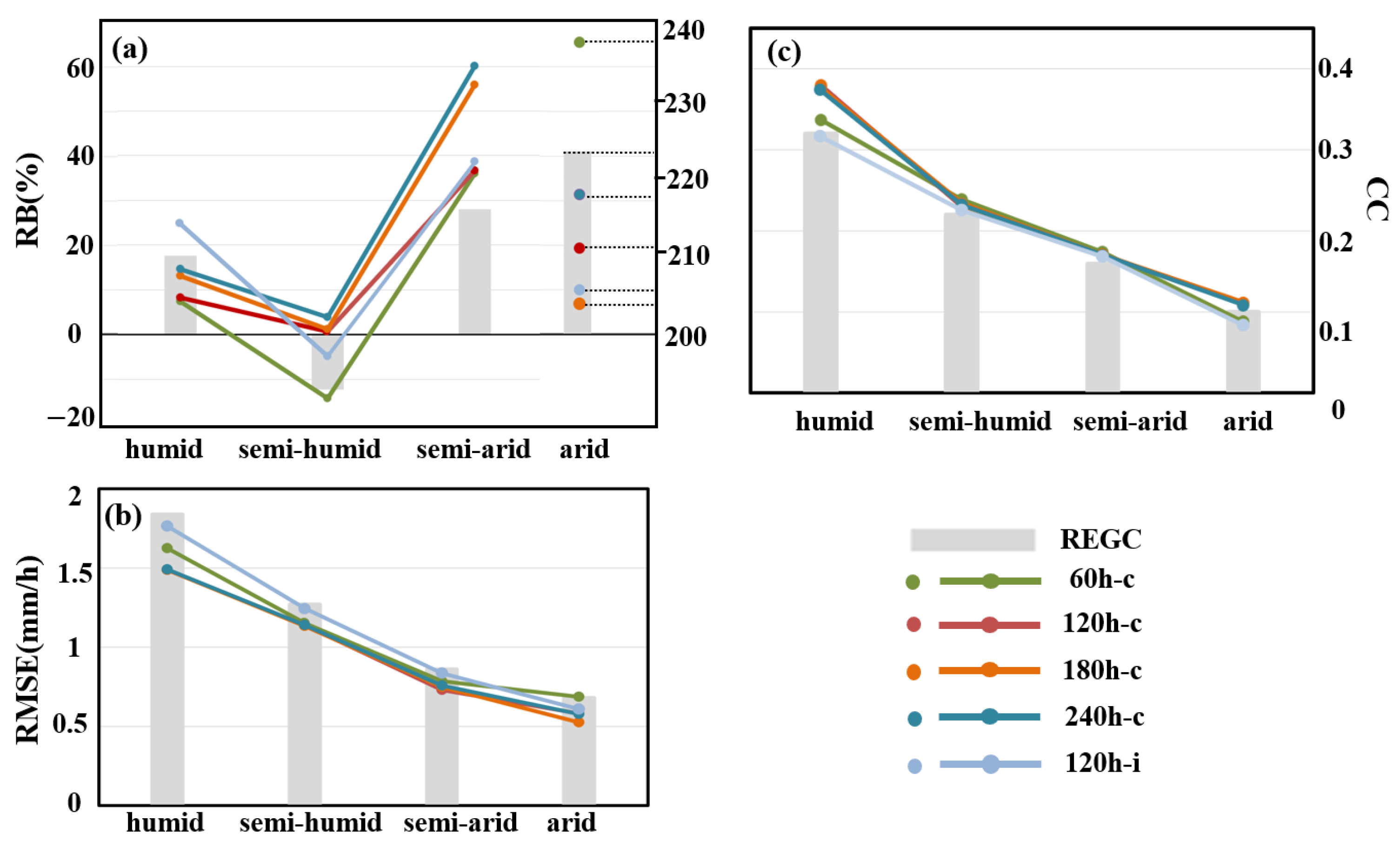
5.1. Different Training Data Lengths for the SISP Approach and the Threshold Selection

In this section, time series of different lengths are used as time windows to construct the error calibration model and summarize the error statistical indicators of the corrected SISP-RT products in mainland China and each climate zone (Table 3, Figure 12), so as to discuss the influence of lengths of training data on the robustness of the SISP method. Time windows are mainly divided into two categories: continuous time series and interval time series. The former is to choose the first n consecutive hours (abbreviated as n h-c) forward from the uncorrected hour t as a time window, such as 60 h-c, 120 h-c, 180 h-c, 240 h-c. The latter adopts the “interval” of 120 h (abbreviated as 120 h-i) proposed by Yu et al. [43] as the time window, which is composed of 120 h by taking 20 days from the current date forward and 6 times per day from the current moment forward.
Analyzed from the perspective of mainland China (Table 3), the SISP algorithm constructed based on continuous time series is more advantageous in reducing the bias compared with the interval corrected series, where the biases of the original data were reduced by 68–72%; in contrast, the satellite precipitation estimates corrected with 120 h-i training data have higher biases in Mainland China. Meanwhile, we found that either too short or too long a training period affects the accuracy of the algorithm, and the overall performance showed that the sensitivity of RMSE and CC to time length decreases and RB tends to increase with the increase in training period time. Similarly, the correction effect of SISP in each climate region was also related to the duration of the training period (Figure 12). Precipitation products corrected by the 60 h-c (green curve) and 120 h-i (light blue curve) training lengths have substantially poorer accuracy than those corrected by other training lengths, especially with greater instability in RB, and are more likely to lead to apparent overestimation or underestimation of precipitation in humid and semi-humid regions. This may be explained mainly from two aspects: on the one hand, because a shorter training period (60 h-c) would lead to too little amount of valid sample data available, the sample data to meet the threshold requirements must be acquired by continuously expanding the spatial window, which would easily lead to overfitting of the correction algorithm and affect the algorithm accuracy. On the other hand, the longer training period (e.g., 120 h-i) consists of a time window spanning 20 days, and the greater frequency of changes in the hourly-scale sample data makes the error characteristics of the sample data weakly correlated with the current precipitation data, which likewise affects the accuracy of the SISP method.
In investigating the influence of different lengths of training periods on the error calibration model above, thresholds were set for the number of samples within each climate region whether to perform the calibration model or not (Table 4). Different thresholds are beneficial to reduce the time complexity of the algorithm while giving full consideration to the influence of the SISP algorithm in reducing the spatial and temporal heterogeneity of precipitation, where the threshold for the humid region is 50% of the length of the time window and that of the other climate regions is in decreasing order. The rainfall within each climate region is varied and the distribution of stations is not uniform (Figure 1b). The number of stations in the humid region is dense and the rainfall is large, so the correction model in the humid region can easily collect a sufficient number of sample data by only the initial spatial search window (9 × 9), while the stations in the western arid and semi-arid regions are sparse and the rainfall is small, thus the spatial window needs to be continuously expanded to obtain the same number of sample data. However, the number of effective samples in the arid or semi-arid regions on the hourly scale is extremely small, which easily leads to an infinite expansion of the spatial window, and the time complexity of the algorithm increases subsequently. Therefore, it is necessary to set thresholds according to the density of stations within the climate region and the magnitude of rainfall, in an effort to avoid reducing the temporal efficiency of the algorithm resulting from the infinite expansion of the spatial window, and also to ensure the correlation of valid samples within the spatial region.

5.2. Strengths and Limitations of the Method

In a study of bias correction based on statistical relationships between station data and satellite precipitation data, Tian et al. [25] pointed out that consistent error characteristics in satellite precipitation estimates are a prerequisite for correction, and inconsistency in errors between the training and correction periods can easily lead to overcorrection. For example, in this paper, Table 2 shows that REGC overestimates precipitation throughout the summer (RB = 112%) in mainland China, but as seen in the time-series plot of RB (Figure 9a), REGC suffers overestimation of precipitation in July, while it mainly presents underestimation in June and August, indicating that the error characteristics of satellite precipitation estimates are inconsistent within each summer month.
Most of the existing correction methods use fixed parameters to correct the bias on the seasonal scale, which easily causes uncertainty. The SISP algorithm proposed in this paper makes the acquired training samples vary with the location of the target grid by setting a spatial window for the dynamic search of the target grid. Thus, it can ensure that the precipitation data at different times and different grid locations have matching correction parameters, further minimizing the impact of error inconsistency on bias correction. At the same time, the error characteristics of REGC are different in each climate region in summer; for instance, REGC tends to underestimate precipitation in semi-humid regions and overestimate precipitation in other climate regions (Table 2). The SISP algorithm also takes this into account. The new method sets a threshold for the number of samples for each climate region and adaptively adjusts the size of the spatial window so that it can rate the parameters at the spatial scale of climate regions and reduce the effect of spatial and temporal heterogeneity of precipitation. The spatio-temporal performance of the satellite precipitation products before and after calibration also proves that the SISP method can indeed effectively reduce the bias but is susceptible to the influence of climate regions. SISP has the best calibration effect in the humid region, while it can only improve the negative bias and can hardly reduce the positive bias in the arid and semi-arid regions. This is mainly due to the sparse sites and light rainfall in arid and semi-arid regions, which leads to a spatial window continuously expanding the search range to obtain sufficient sample data, resulting in increased spatial dissimilarity and reduced correlation between sample data, which tends to affect the performance of the revised algorithm. In addition, based on sequential processing, SISP updates the original data with new corrected data to train and obtains new information for correction, which can improve the accuracy of the parameters. The time-series plot of hourly average precipitation deviations in Figure 6 shows that the effectiveness of the SISP algorithm in revising the deviations increases with increasing time series.
In general, the SISP algorithm can have the advantage of reducing the bias, but at present, it only improves and does not completely eliminate the bias. The correction effect of SISP on satellite precipitation estimates varies in different regions, months, and at various precipitation intensities. Therefore, in order to better exploit the advantages of this correction algorithm, a suitable spatial and temporal window needs to be selected by practice to avoid shorter or longer correction sequences to reduce the effectiveness of the algorithm for bias correction.

5.3. Application Prospects

Mainland China is susceptible to warm and humid southwest monsoon airflow, resulting in precipitation events occurring mainly in summer when precipitation is abundant and differs significantly between inland and coastal areas. Therefore, only summer is chosen as the study time in this paper. Since the spatial and temporal window of SISP is adaptive and can be automatically resized not only according to the spatio-temporal variability of precipitation within the climate region but can also be also modified according to the seasonal characteristics of precipitation, the model can be applied to the error adjustment of satellite precipitation for the other three seasons according to specific needs.
Last but not least, this paper only practices the applicability of the SISP algorithm at the spatial scale of mainland China and four climatic zones; however, many watersheds in summer are very likely to be flooded caused by abundant and uneven precipitation. Therefore, the advantages of high spatial and temporal resolution (5 min/4 km) of REGC data and the potential of the SISP algorithm to correct bias on a time-by-time basis can be combined in the future to further divide the study area into finer watershed scales, which is very important for runoff simulation and flood warning studies in various watersheds in China and even in other countries and regions in the world.
Finally, the error-correction scheme is effective based on the consistency of the errors in short-term accumulated precipitation data over a certain spatial range. In the future, it can be applied to the error correction of other satellite precipitation estimates at hourly scales by modifying the threshold value as well as the training period.

6. Conclusions

In this paper, we proposed and practiced a self-adaptive ill-posed least squares bias-correction method based on sequential processing to hour-by-hour correct satellite precipitation estimates, which considers the relationship between climate region, precipitation intensity, topography, and precipitation errors from the perspective of reducing the effect of spatial and temporal variability of precipitation for bias correction. Firstly, based on the idea of sequential processing, the corrected data are updated hour by hour instead of the original data to obtain the dynamically changing short time-series time window, and secondly, by setting the dynamic search window, the sample data within the spatial window changes with the change of the target grid position, and finally the satellite precipitation data can be corrected hour by the hour based on the dynamic parameters. The main conclusions are as follows:
(1)
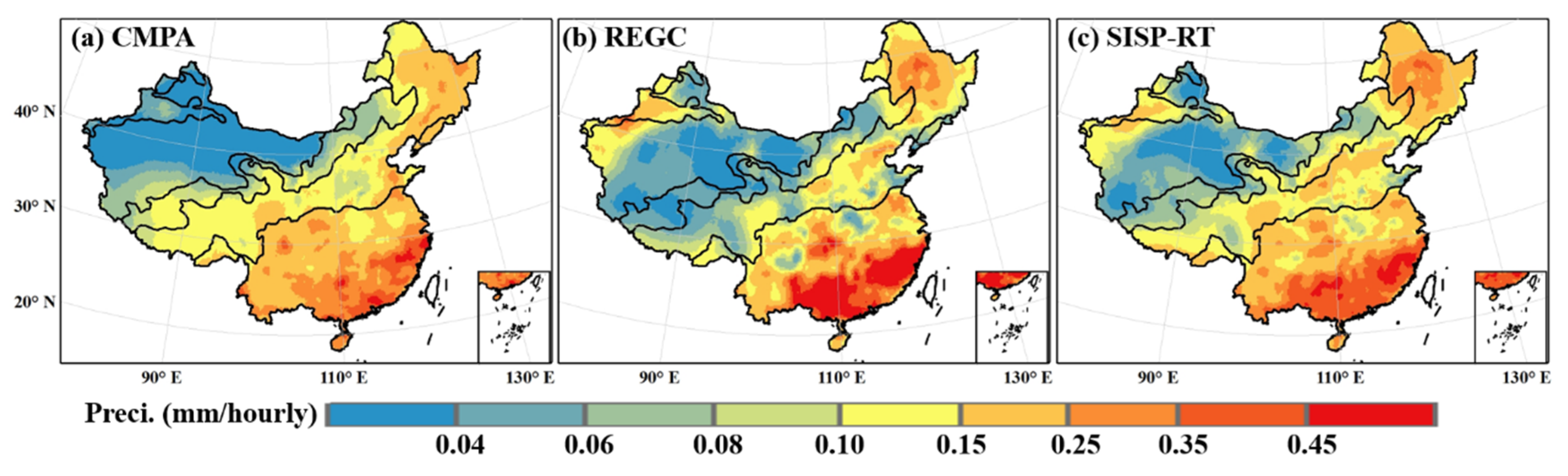
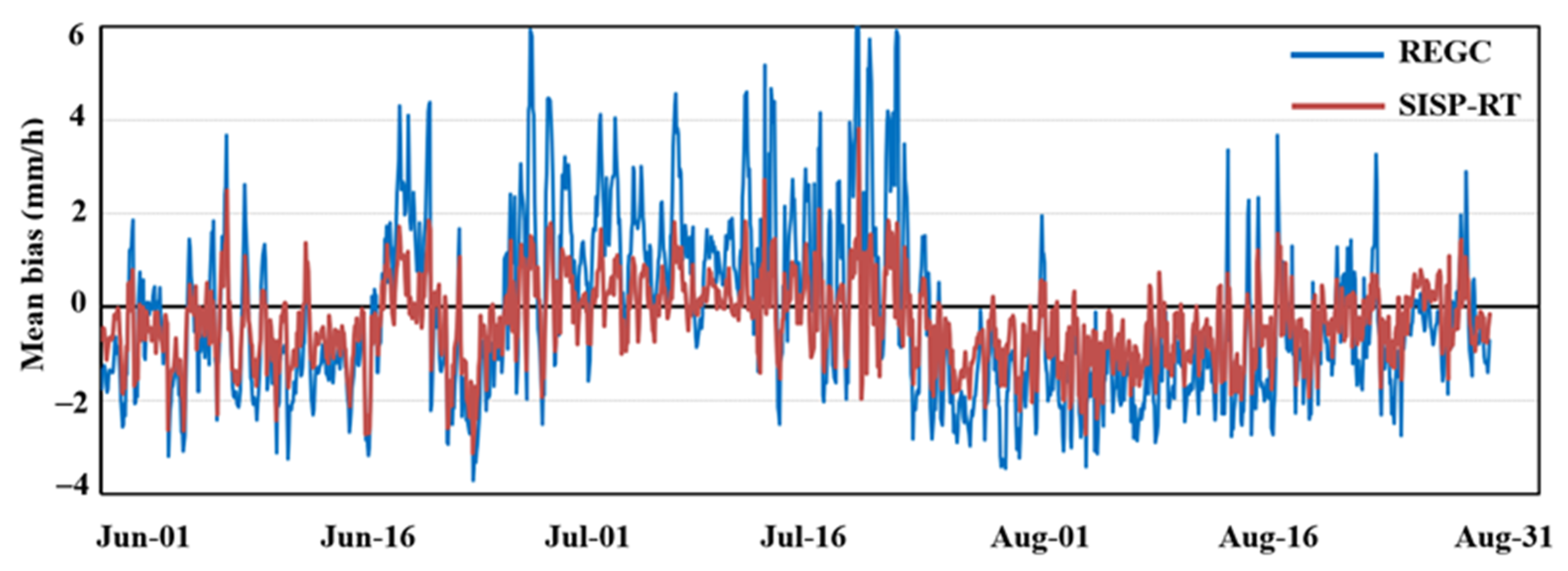
In the analysis of the hourly average precipitation of precipitation products, the hourly average precipitation of REGC is higher than that of CMPA in most areas of mainland China, while the quantitative values of SISP-RT are more similar to those of CMPA, indicating the advantage of the SISP method in correcting rainfall. In the time-series plot of the hourly mean bias, it is found that the SISP method corrects the biases significantly better in the middle and later stages of the time series than in the initial stage, which may be related to the addition of the corrected satellite precipitation data to the training sample to improve the accuracy of the correction parameters.
(2)
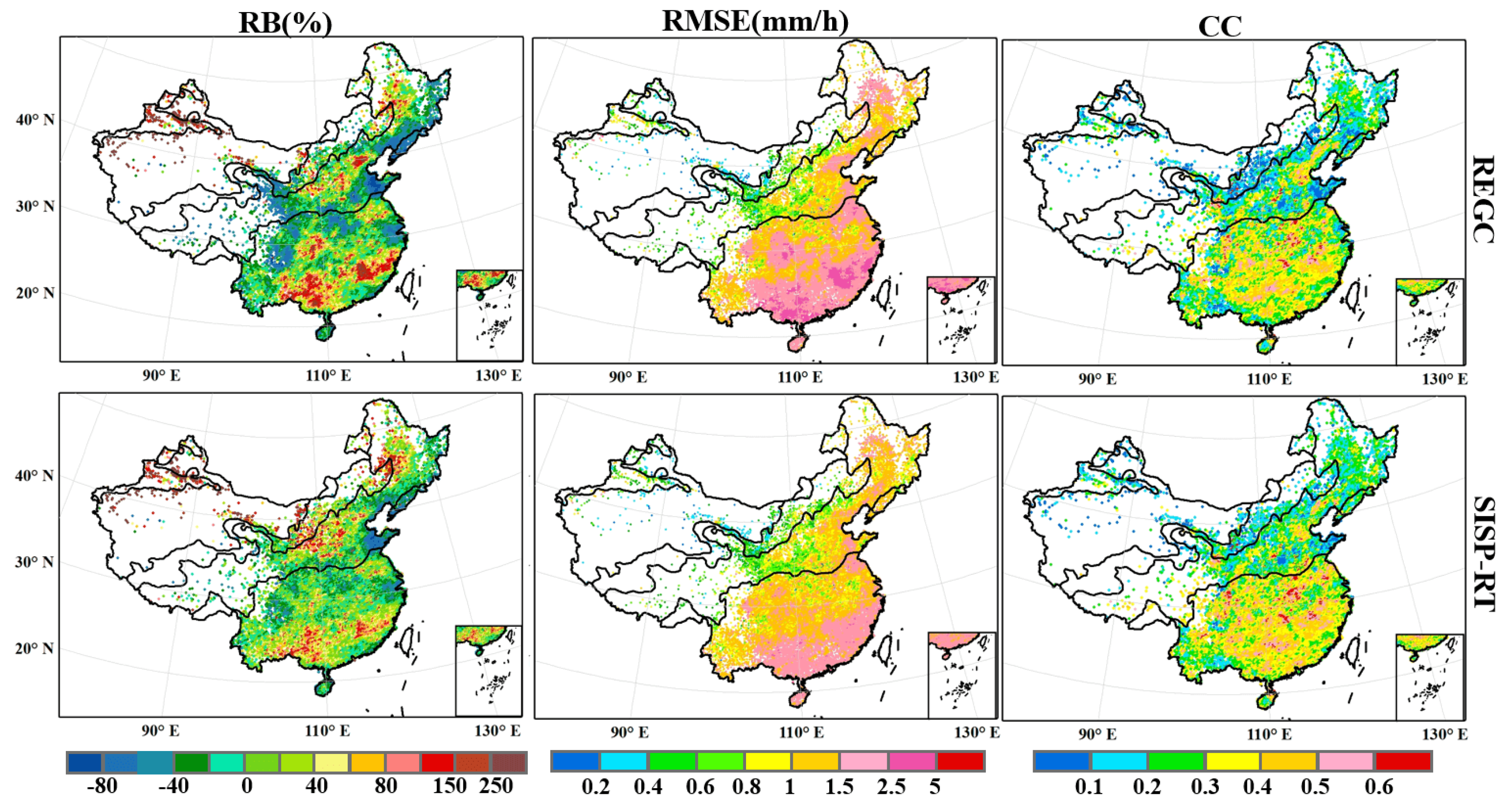
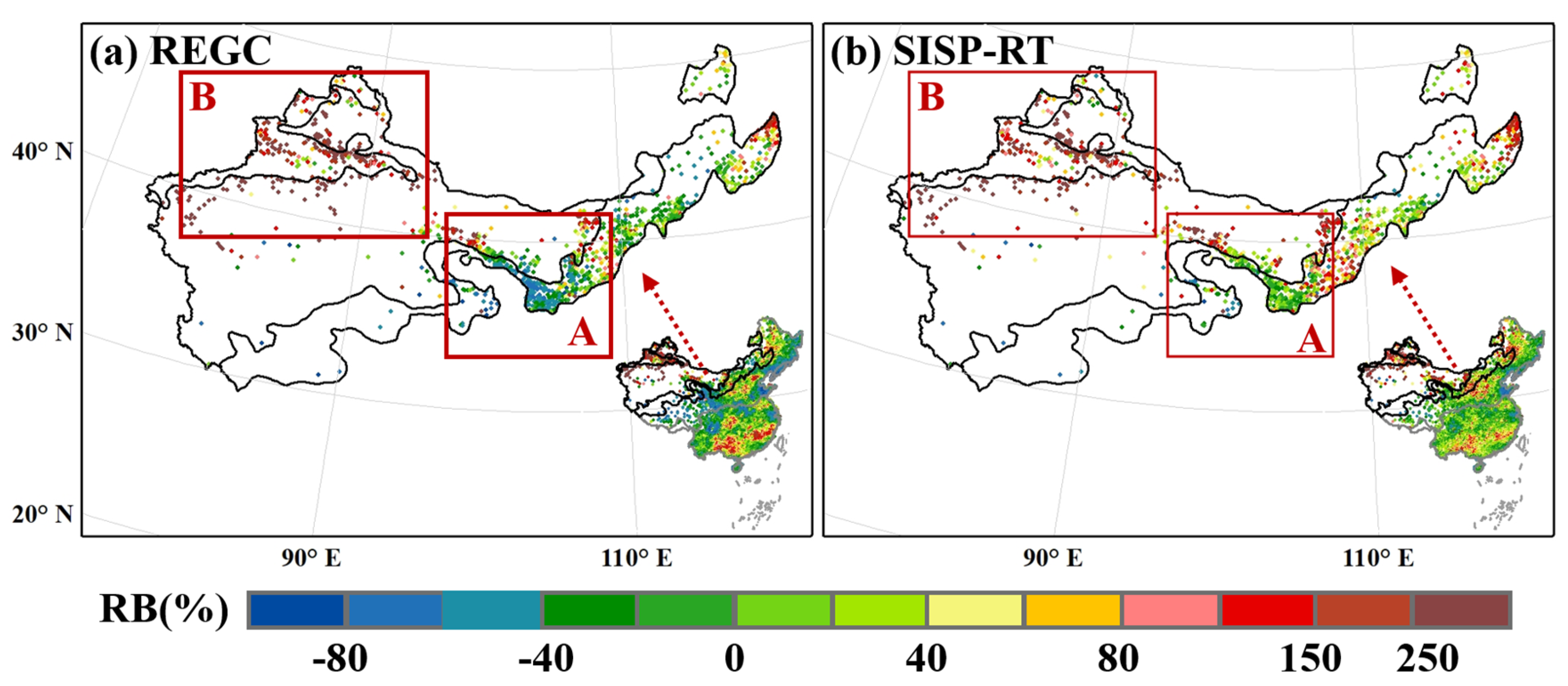
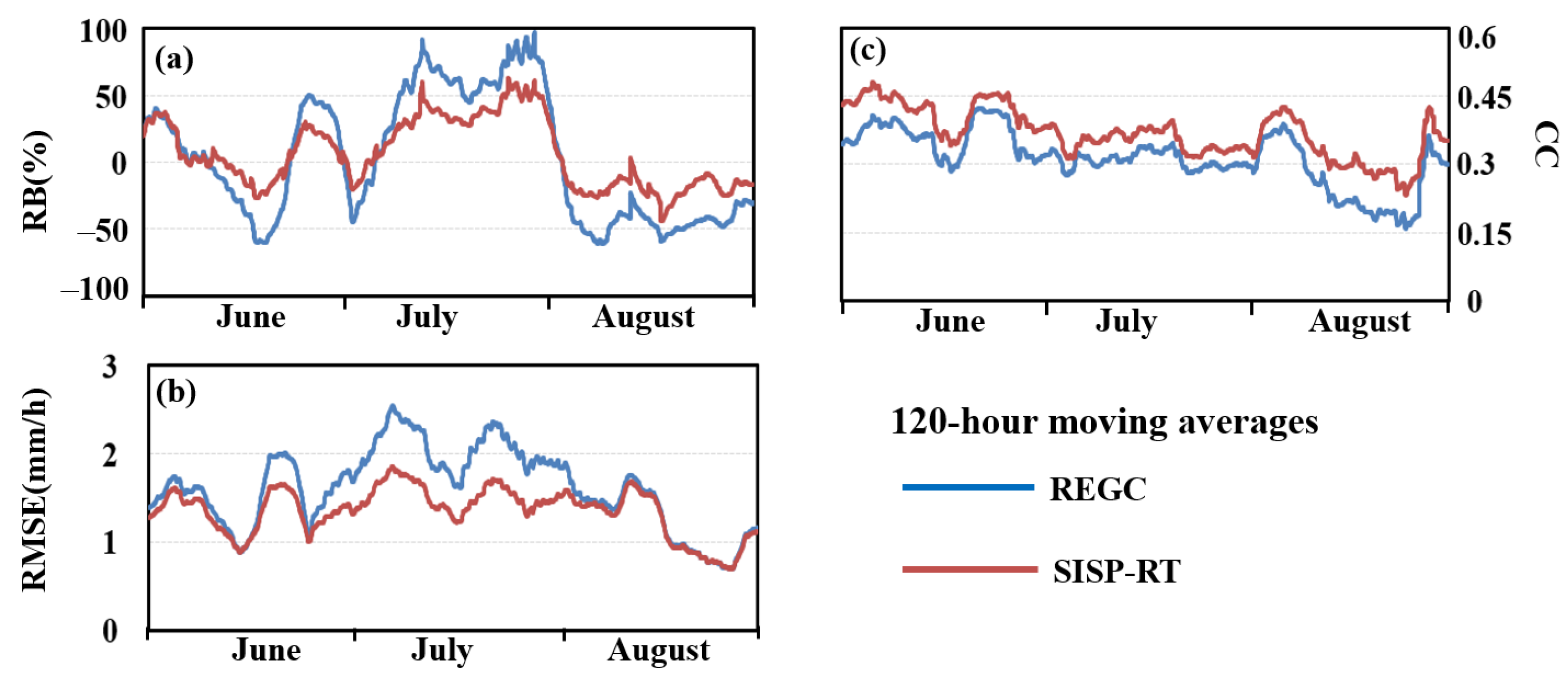
In the spatial analysis, the SISP algorithm can effectively reduce the error of the original REGC in mainland China and mainly fix the biases of the original REGC in the central regions of the humid and semi-humid regions. Compared with REGC, the RB of SISP-RT is reduced by 52% in the humid region, but further improvement is needed in reducing the bias in the arid and semi-arid regions. In the temporal analysis, the RB and RMSE of REGC show a clear pattern of monthly variation, and the variation of RB and RMSE curves of SISP-RT is obviously decreased after correction.
(3)
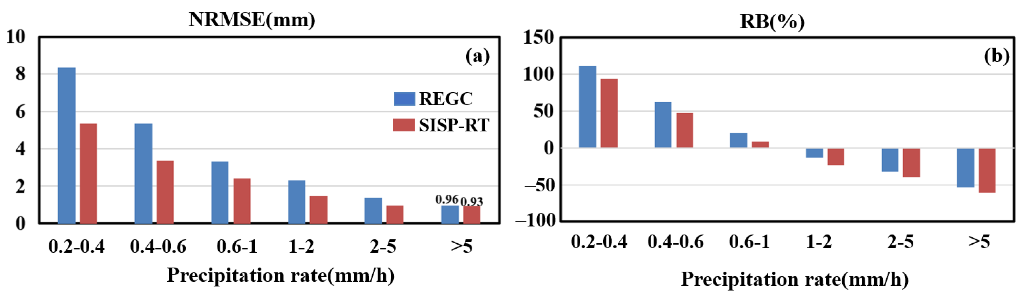
In terms of precipitation intensity, the original REGC exhibits overestimation for low rain intensity (0.2–1 mm/h) and underestimation for high rain intensity (>1 mm/h). The SISP algorithm remarkably improves the overestimation of low rain intensity from the original data but tends to overcorrect for rainfall rates above 1 mm/h leading to more severe underestimation.
(4)
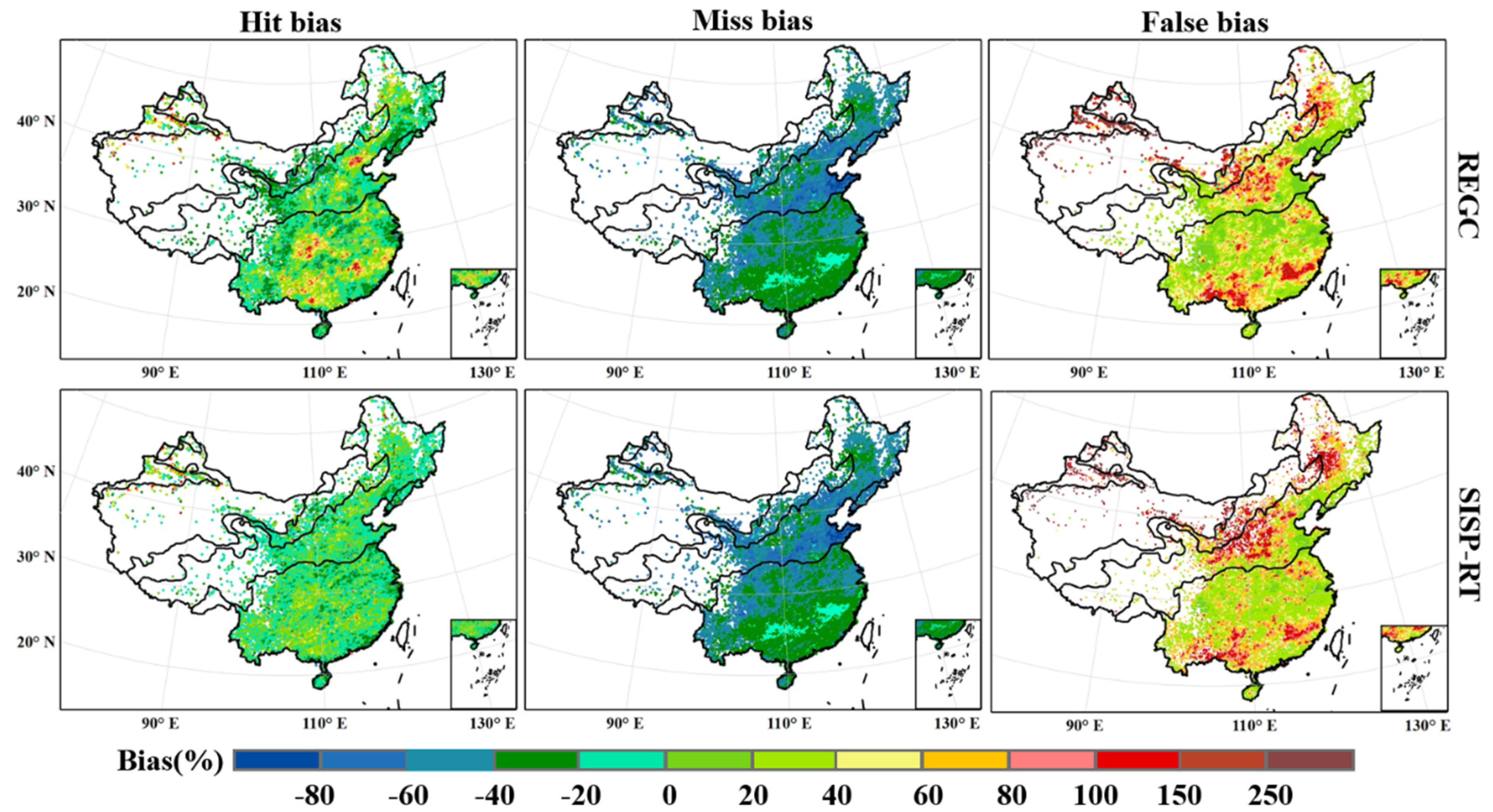
The contribution and problems of the SISP algorithm in correcting each error component were further clarified by error decomposition. The SISP algorithm can effectively reduce hit biases in the real-time corrected data and has a better effect on the higher positive hit biases (from more than 80% to about 20%). However, limited by the fact that the precipitation in some regions is outside the effective correction range of miss biases and false biases, the algorithm basically cannot improve the miss bias and the false bias of the original satellite precipitation products.

Author Contributions

Conceptualization, J.L.; methodology, J.L., Z.S., and H.W.; software, J.L.; validation, J.L.; formal analysis, J.L.; resources, J.L.; writing—original draft preparation, J.L.; writing—review and editing, B.Y. and Y.Y.; visualization, J.L.; funding acquisition, B.Y. All authors have read and agreed to the published version of the manuscript.

Funding

This research was funded by the National Key R&D Program of China (2021YFB3900601).

Data Availability Statement

The data are available from the corresponding authors upon reasonable request.

Acknowledgments

The authors are grateful to the National Satellite Meteorological Center (NSMC) for providing FengYun 4A (FY4A) products and thankful to the China Meteorological Administration (CMA) for providing CMPA data. The authors would also like to express our appreciation for the constructive comments and suggestions of all anonymous reviewers and editors.

Conflicts of Interest

The authors declare no conflict of interest.

References

  1. Trenberth, K.E.; Dai, A.; Rasmussen, R.M.; Parsons, D.B. The changing character of precipitation. Bull. Am. Meteorol. Soc. 2003, 84, 1205–1217. [Google Scholar] [CrossRef]
  2. Kidd, C.; Bauer, P.; Turk, J.; Huffman, G.; Joyce, R.; Hsu, K.; Braithwaite, D. Intercomparison of high-resolution precipitation products over northwest Europe. J. Hydrometeorol. 2012, 13, 67–83. [Google Scholar] [CrossRef] [Green Version]
  3. Allen, M.R.; Ingram, W.J. Constraints on future changes in climate and the hydrologic cycle. Nature 2002, 419, 224–232. [Google Scholar] [CrossRef] [PubMed]
  4. Veerakachen, W.; Raksapatcharawong, M. Rainfall estimation for real time flood monitoring using geostationary meteorolog-ical satellite data. Adv. Space Res. 2015, 56, 1139–1145. [Google Scholar] [CrossRef] [Green Version]
  5. Hou, A.Y.; Kakar, R.K.; Neeck, S.; Azarbarzin, A.A.; Kummerow, C.D.; Kojima, M.; Oki, R.; Nakamura, K.; Iguchi, T. The global precipitation measurement mission. Bull. Am. Meteorol. Soc. 2014, 95, 701. [Google Scholar] [CrossRef]
  6. Boushaki, F.I.; Hsu, K.; Sorooshian, S.; Park, G.; Mahani, S.; Shi, W. Bias adjustment of satellite precipitation estimation using ground-based measurement: A case study evaluation over the southwestern united states. J. Hydrometeorol. 2009, 10, 1231–1242. [Google Scholar] [CrossRef]
  7. Yilmaz, K.K.; Adler, R.F.; Tian, Y.; Hong, Y.; Pierce, H.F. Evaluation of a satellite-based global flood monitoring system. Int. J. Remote Sens. 2010, 31, 3763–3782. [Google Scholar] [CrossRef]
  8. Li, Z.; Yang, D.; Hong, Y. Multi-scale evaluation of high-resolution multi-sensor blended global precipitation products over the Yangtze River. J. Hydrol. 2013, 500, 157–169. [Google Scholar] [CrossRef]
  9. Ma, Y.; Zhang, Y.; Yang, D.; Bin Farhan, S. Precipitation bias variability versus various gauges under different climatic condi-tions over the Third Pole Environment (TPE) region. Int. J. Climatol. 2015, 35, 1201–1211. [Google Scholar] [CrossRef]
  10. Tang, G.; Behrangi, A.; Long, D.; Li, C.; Hong, Y. Accounting for spatiotemporal errors of gauges: A critical step to evaluate gridded precipitation products. J. Hydrol. 2018, 559, 294–306. [Google Scholar] [CrossRef] [Green Version]
  11. Yong, B.; Hong, Y.; Ren, L.-L.; Gourley, J.J.; Huffman, G.J.; Chen, X.; Wang, W.; Khan, S.I. Assessment of evolving TRMM-based multisatellite real-time precipitation estimation methods and their impacts on hydrologic prediction in a high latitude basin. J. Geophys. Res. Atmos. 2012, 117, D9. [Google Scholar] [CrossRef] [Green Version]
  12. Behrangi, A.; Hsu, K.; Imam, B.; Sorooshian, S.; Huffman, G.J.; Kuligowski, R.J. PERSIANN-MSA: A precipitation estimation method from satellite-based multispectral analysis. J. Hydrometeorol. 2009, 10, 1414–1429. [Google Scholar] [CrossRef]
  13. Tapiador, F.J.; Turk, F.J.; Petersen, W.; Hou, A.Y.; García-Ortega, E.; Machado, L.A.T.; Angelis, C.F.; Salio, P.; Kidd, C.; Huffman, G.J.; et al. Global precipitation measurement: Methods, datasets and applications. Atmos. Res. 2012, 104, 70–97. [Google Scholar] [CrossRef]
  14. Jianyun, Z. Review and reflection on China’s hydrological forecasting techniques. Adv. Water Sci. 2010, 21, 435–443. [Google Scholar] [CrossRef]
  15. Hanqing, C.; Bin, Y.; Emmanuel, K.P.; Leyang, W.; Yang, H. Global component analysis of errors in three satellite-only global precipitation estimates. Hydrol. Earth Syst. Sci. 2021, 25, 3087–3104. [Google Scholar] [CrossRef]
  16. Sorooshian, S.; Hsu, K.L.; Gao, X.; Gupta, H.V.; Imam, B.; Braithwaite, D. Evaluation of PERSIANN system satellite-based es-timates of tropical rainfall. Bull. Am. Meteorol. Soc. 2000, 81, 2035–2046. [Google Scholar] [CrossRef]
  17. Zhang, X.; Tang, Q. Combining satellite precipitation and long-term ground observations for hydrological monitoring in China. J. Geophys. Res.-Atmos. 2015, 120, 6426–6443. [Google Scholar] [CrossRef] [Green Version]
  18. Lu, X.; Tang, G.; Wang, X.; Liu, Y.; Jia, L.; Xie, G.; Li, S.; Zhang, Y. Correcting GPM IMERG precipitation data over the Tianshan Mountains in China. J. Hydrol. 2019, 575, 1239–1252. [Google Scholar] [CrossRef]
  19. Zhou, Z.; Guo, B.; Xing, W.; Zhou, J.; Xu, F.; Xu, Y. Comprehensive evaluation of latest GPM era IMERG and GSMaP precipita-tion products over mainland China. Atmos. Res. 2020, 246, 105132. [Google Scholar] [CrossRef]
  20. Lu, D.; Yong, B. Evaluation and hydrological utility of the latest GPM IMERG V5 and GSMaP V7 precipitation products over the Tibetan Plateau. Remote Sens. 2018, 10, 2022. [Google Scholar] [CrossRef] [Green Version]
  21. Moazami, S.; Na, W.; Najafi, M.R.; de Souza, C. Spatiotemporal bias adjustment of IMERG satellite precipitation data across Canada. Adv. Water Resour. 2022, 168, 104300. [Google Scholar] [CrossRef]
  22. Ma, Z.; Xu, J.; Zhu, S.; Yang, J.; Tang, G.; Yang, Y.; Shi, Z.; Hong, Y. AIMERG: A new Asian precipitation dataset (0.1 de-grees/half-hourly, 2000–2015) by calibrating the GPM-era IMERG at a daily scale using APHRODITE. Earth Syst. Sci. Data 2020, 12, 1525–1544. [Google Scholar] [CrossRef]
  23. Yang, F.; Wang, W.; Lu, H.; Yang, K.; Tian, F. Improving GPM precipitation data over yarlung zangbo river basin using smap soil moisture retrievals. In Proceedings of the IGARSS 2018–2018 IEEE International Geoscience and Remote Sensing Symposium, Valencia, Spain, 22–27 July 2018; pp. 3047–3050. [Google Scholar]
  24. Nie, S.; Wu, T.; Luo, Y.; Deng, X.; Shi, X.; Wang, Z.; Liu, X.; Huang, J. A strategy for merging objective estimates of global daily precipitation from gauge observations, satellite estimates, and numerical predictions. Adv. Atmos. Sci. 2016, 33, 889–904. [Google Scholar] [CrossRef]
  25. Tian, Y.; Peters-Lidard, C.D.; Eylander, J.B. Real-Time bias reduction for satellite-based precipitation estimates. J. Hydromete-orol. 2010, 11, 1275–1285. [Google Scholar] [CrossRef]
  26. Deng, P.; Zhang, M.; Guo, H.; Xu, C.; Bing, J.; Jia, J. Error analysis and correction of the daily GSMaP products over Hanjiang River Basin of China. Atmos. Res. 2018, 214, 121–134. [Google Scholar] [CrossRef]
  27. Choubin, B.; Khalighi-Sigaroodi, S.; Mishra, A.; Goodarzi, M.; Shamshirband, S.; Ghaljaee, E.; Zhang, F. A novel bias correction framework of TMPA 3B42 daily precipitation data using similarity matrix/homogeneous conditions. Sci. Total Environ. 2019, 694, 133680. [Google Scholar] [CrossRef]
  28. Sun, W.; Sun, Y.; Li, X.; Wang, T.; Wang, Y.; Qiu, Q.; Deng, Z. Evaluation and correction of GPM IMERG precipitation products over the capital circle in northeast China at multiple spatiotemporal scales. Adv. Meteorol. 2018, 2018, 4714173. [Google Scholar] [CrossRef]
  29. Yang, Z.; Hsu, K.; Sorooshian, S.; Xu, X.; Braithwaite, D.; Verbist, K.M.J. Bias adjustment of satellite-based precipitation estima-tion using gauge observations: A case study in Chile. J. Geophys. Res. Atmosp. 2016, 121, 3790–3806. [Google Scholar] [CrossRef] [Green Version]
  30. Shen, Z.; Yong, B.; Gourley, J.J.; Qi, W. Real-time bias adjustment for satellite-based precipitation estimates over Mainland China. J. Hydrol. 2021, 596, 126133. [Google Scholar] [CrossRef]
  31. Chen, H.; Yong, B.; Gourley, J.J.; Wen, D.; Qi, W.; Yang, K. A novel real-time error adjustment method with considering four factors for correcting hourly multi-satellite precipitation estimates. IEEE Trans. Geosci. Remote 2022, 60, 4105211. [Google Scholar] [CrossRef]
  32. Yin, J.B.; Guo, S.L.; Gu, L. Thermodynamic response of precipitation extremes to climate change and its impacts on floods over China. Chin. Sci. Bull. 2021, 66, 4315–4325. [Google Scholar] [CrossRef]
  33. Degefu, M.A.; Bewket, W. Variability and trends in rainfall amount and extreme event indices in the Omo-Ghibe River Basin, Ethiopia. Reg. Environ. Chang. 2014, 14, 799–810. [Google Scholar] [CrossRef]
  34. Niu, N.; Jiang, X.; Zhang, X. Application of FY-4 satellite products in the analysis of a rainstorm weather process. Satell. Appl. 2022, 3, 42–48. [Google Scholar]
  35. Xian, D.; Ren, S.; Shao, J. Application of Fengyun Meteorological Satellite in Flood Season Disaster Pevention and Mitigation. Satell. Appl. 2020, 34, 13–18. [Google Scholar] [CrossRef]
  36. Lu, H.; Huang, Z.; Ding, L.; Lu, T.; Yuan, Y. Calibrating FY4A QPE using CMPA over Yunnan-Kweichow Plateau in summer 2019. Eur. J. Remote Sens. 2021, 54, 476–486. [Google Scholar] [CrossRef]
  37. Ren, J.; Xu, G.R.; Zhang, W.G.; Leng, L.; Xiao, Y.J.; Wan, R.; Wang, J.C. Evaluation and improvement of FY-4A AGRI quantita-tive precipitation estimation for summer precipitation over complex topography of western China. Remote Sens. 2021, 13, 4366. [Google Scholar] [CrossRef]
  38. Yin, T.; Yin, S.; Li, F. Relationship between the summer extreme precipitation in the south and north of the qinling Mountains and the western pacific subtropical high. Arid. Zone Res. 2019, 36, 1379–1390. [Google Scholar] [CrossRef]
  39. Zhang, C. Changes in the characteristics of subtropical high pressure in the western Pacific Ocean during summer and its im-pact on summer precipitation in China over the past 60 years. In Proceedings of the Innovation-Driven Development Improving Meteorological Disaster Defense Capability-The 30th Annual Meeting of the Chinese Meteorological Society, Nanjing, China, 9 March 2013; pp. 310–322. [Google Scholar]
  40. Yong, B.; Chen, B.; Tian, Y.; Yu, Z.; Hong, Y. Error-component analysis of TRMM-Based multi-satellite precipitation estimates over Mainland China. Remote Sens. 2016, 8, 440. [Google Scholar] [CrossRef] [Green Version]
  41. Shen, Y.; Zhao, P.; Pan, Y.; Yu, J. A high spatiotemporal gauge-satellite merged precipitation analysis over China. J. Geophys. Res.-Atmos. 2014, 119, 3063–3075. [Google Scholar] [CrossRef]
  42. Pan, Y.; Shen, Y.; Yu, J. Analysis of The combined gauge-satellite hourly precipitation over China based on the OI technique. Acta Meteorol. Sin. 2012, 70, 1381–1389. [Google Scholar] [CrossRef]
  43. Yu, J.; Shen, Y.; Pan, Y. Improvement of satellite-based precipitation estimates over china based 0n probability density func-tion matching method. J. Appl. Meteorol. Sci. 2013, 24, 544–553. [Google Scholar]
  44. Shen, Y.; Pan, Y.; Yu, J. Quality assessment of hourly merged precipitation product over China. Trans. Atmos. Sci. 2013, 36, 37–46. [Google Scholar] [CrossRef]
  45. Yu, J.; Shen, Y.; Pan, Y. Comparative assessment between the daily merged precipitation dataset over China and The Worlds Popular Counterparts. Acta Meteorol. Sin. 2015, 73, 394–410. [Google Scholar]
  46. National Satellite Meteorological Center. FengYun 4A. Available online: https://fy4.nsmc.org.cn/nsmc/cn/satellite/FY4A.html. (accessed on 23 December 2022).
  47. Zhong, Y. Evaluation and verification of FY-4A satellite quantitative precipitation estimation product. J. Agric. Catastroph. 2021, 11, 96–98. [Google Scholar]
  48. Nie, S.; Luo, Y.; Zhu, J. Trends and scales of observed soil moisture variations in China. Adv. Atmos. Sci. 2008, 25, 43–58. [Google Scholar] [CrossRef]
  49. Chen, H.; Yong, B.; Shen, Y.; Liu, J.; Hong, Y.; Zhang, J. Comparison analysis of six purely satellite-derived global precipitation estimates. J. Hydrol. 2020, 581, 124376. [Google Scholar] [CrossRef]
  50. Lu, C.; Ye, J.; Fang, G.; Huang, X.; Yan, M. Assessment of GPM IMERG Satellite Precipitation Estimation under Complex Cli-matic and Topographic Conditions. Atmosphere 2021, 12, 780. [Google Scholar] [CrossRef]
  51. Gao, Z.; Huang, B.; Ma, Z.; Chen, X.; Qiu, J.; Liu, D. Comprehensive comparisons of state-of-the-art gridded precipitation es-timates for hydrological applications over southern China. Remote Sens. 2020, 12, 3997. [Google Scholar] [CrossRef]
  52. Zhang, F.; Chai, Y.; Chai, H.; Ding, L. lmproving the ll-posed problems of the least squares attitude estimation with GNSS multi-antennas using. J. Navig. Position. 2015, 3, 85–88. [Google Scholar] [CrossRef]
  53. Tian, Y.; Peters-Lidard, C.D.; Eylander, J.B.; Joyce, R.J.; Huffman, G.J.; Adler, R.F.; Hsu, K.L.; Turk, F.J.; Garcia, M.; Zeng, J. Component analysis of errors in satel-lite-based precipitation estimates. J. Geophys. Res. Atmos. 2009, 114, D24. [Google Scholar] [CrossRef] [Green Version]
  54. Skoien, J.O.; Bloschl, G.; Western, A.W. Characteristic space scales and timescales in hydrology. Water. Resour. Res. 2003, 39, 10. [Google Scholar] [CrossRef]
  55. Wu, H.; Yong, B.; Shen, Z.; Qi, W. Comprehensive error analysis of satellite precipitation estimates based on Fengyun-2 and GPM over Mainland China. Atmos. Res. 2021, 263, 105805. [Google Scholar] [CrossRef]
Figure 1. (a) Topographic map of China; (b) Spatial distributions of rain gauge stations and the climate regions over Mainland China.
Remotesensing 15 01819 g001
Figure 2. The flowchart of adjusting hourly REGC.
Remotesensing 15 01819 g002
Figure 3. Diagram of the temporal window.
Remotesensing 15 01819 g003
Figure 4. Diagram of the spatial window.
Remotesensing 15 01819 g004
Figure 5. Spatial distribution of mean hourly precipitation for CMPA, REGC, and SISP-RT (June to August 2019).
Remotesensing 15 01819 g005
Figure 6. Time series of mean biases for REGC and SISP-RT at hourly scale in June–August 2019.
Remotesensing 15 01819 g006
Figure 7. Spatial patterns of RB (first column), RMSE (second column), and CC (third column) of the REGC and SISP-RT against the CMPA over Mainland China.
Remotesensing 15 01819 g007
Figure 8. Spatial patterns of RB for the REGC and SISP-RT in the semi-arid and arid regions.
Remotesensing 15 01819 g008
Figure 9. Time series of RB (a), RMSE (b), and CC (c) of the REGC and SISP-RT against the CMPA in Jun–Aug 2019. All lines are obtained from 120 h moving averages of the original time series.
Remotesensing 15 01819 g009
Figure 10. The (a) NRMSE and (b) RB of the REGC and SISP-RT at 0.1° spatial and hourly temporal resolution under different precipitation intensities.
Remotesensing 15 01819 g010
Figure 11. Spatial patterns of the three error components (i.e., hit bias (first column), miss bias (second column), false bias (third column)) for the REGC and SISP-RT at 0.1° spatial and hourly temporal resolution over mainland China in June–August 2019.
Remotesensing 15 01819 g011
Figure 12. The RB (a), RMSE (b), and CC (c) of hourly SISP-RT against CMPA at gauged pixels compared with REGC in climate regions under the different lengths of the training period.
Remotesensing 15 01819 g012
Table 1. The list of the evaluation metrics 1.
Statistic IndicesEquationSuitable Value
CC C C = i = 1 n G i G ¯ S i S ¯ i = 1 n G i G ¯ 2 × i = 1 n S i S ¯ 2 1
RMSE R M S E = 1 n × i = 1 n S i G i 2 0
RB R B = i = 1 n S i G i i = 1 n G i × 100 % 0
Hit bias H i t   b i a s = i = 1 n S H G H i = 1 n G i × 100 % 0
Miss bias M i s s   b i a s = i = 1 n S M G M i = 1 n G i × 100 % 0
False bias F a l s e   b i a s = i = 1 n S F G F i = 1 n G i × 100 % 0
1 Notation: n refers to the total number of samples, G i   refers to ground data, S i refers to satellite data, G ¯ refers to ground precipitation average, S ¯ refers to satellite precipitation average, H refers to the number of precipitation detected by both satellite and ground stations, M refers to the number of precipitation detected by ground stations but not by satellite, and F refers to the number of precipitation detected by satellite but not by ground stations.
Table 2. The summary of the three evaluation indices (RMSE, RB, and CC) for the REGC and SISP-RT for the summers.
Study AreaRMSE (mm/h)RB (%)CC
REGCSISP-RTREGCSISP-RTREGCSISP-RT
Mainland China1.641.3611.23.340.30.35
Humid region1.841.4917.688.150.320.38
Semi-humid region1.271.14−12.330.570.220.26
Semi-arid region0.860.7328.0536.650.160.17
Arid region0.680.58223.22211.030.10.11
Table 3. Metrics of hourly SISP-RT against CMPA at gauged pixels in Mainland China under the different lengths of the training period.
Mainland ChinaRMSE (mm/h)RB (%)CC
REGC1.6411.20.3
60 h-c1.453.190.32
120 h-c1.363.340.35
180 h-c1.363.450.35
240 h-c1.363.590.34
120 h-i1.5718.250.34
Table 4. Thresholds of different training lengths for each climate region.
Climate Regions60 h-c120 h-c180 h-c240 h-c120 h-i
Humid region30609012060
Semi-humid region2050607050
Semi-arid region1030404530
Arid region520303520
Disclaimer/Publisher’s Note: The statements, opinions and data contained in all publications are solely those of the individual author(s) and contributor(s) and not of MDPI and/or the editor(s). MDPI and/or the editor(s) disclaim responsibility for any injury to people or property resulting from any ideas, methods, instructions or products referred to in the content.

