1. Introduction
Interferometric Synthetic Aperture Radar (InSAR) can be used to generate maps of ground displacement covering large regions (100 s of km) with high spatial resolution (a few meters to 10 s of meters) and with accuracies of up to a few mm/y depending on the length of the time series and the surface properties of the region [
1,
2,
3,
4,
5]. InSAR provides all-weather day and night observations that are regularly repeated at intervals of days to weeks [
6]. InSAR has been successfully utilized for surface deformation mapping over the last few decades with a variety of spaceborne SAR systems operating at various wavelengths and resolutions; these include ERS-1/2, ENVISAT ASAR, Radarsat-1/2, JERS1, ALOS/PALSAR, ALOS-2/PALSAR-2, SAOCOM-1, Cosmo-skyMed, Sentinel-1, and TerraSAR-X [
7,
8]. As the data availability and coverage have improved, a wide range of InSAR techniques have been developed to improve the estimation of surface deformation associated with natural processes and human-induced activities such as landslides, earthquakes, volcanoes, groundwater extraction, and mining [
7,
8,
9,
10,
11,
12,
13,
14].
However, InSAR applications in vegetated regions are often severely impacted by the changing scattering properties of the surface [
5,
15,
16]. InSAR coherence, a measure of data quality/noise, is sensitive to the changes in surface backscattering properties and can be influenced by temporal variations due to land cover change, soil moisture, and snow depth [
5,
17,
18,
19,
20]. In addition to the increased level of noise associated with low coherence, the InSAR phase is susceptible to biases and phase artifacts related to atmospheric effects, snow, and vegetation, all of which are prevalent in our study area in the Northeastern United States (
Figure 1). However, there are still deformation signals within the region that are large enough to be studied using InSAR. For example, ALOS1/PALSAR observations show displacement rates as large as 80 mm/year related to subsidence above a salt mine in western New York State [
21,
22]. In this study, we focused on two 3-year time series of InSAR data using two different microwave wavelengths to assess the quality and detection thresholds that are possible in this area. Our work built on numerous other efforts to examine the quality of SAR observations at different wavelengths and develop methods for combining observations from different platforms [
1,
2,
3,
4,
5,
6,
7,
8,
9,
10]. The study area was chosen to test the ability of InSAR to measure a known deformation signal where independent observations of subsidence rates exist at ground control points. The study area also contains a range of land cover types, allowing for further types of intercomparison.
To overcome the limitations that are involved in conventional InSAR, persistent scatterer interferometry (PSI) has been introduced and successfully used to separate surface deformation phase from the other phase artifacts and noise sources [
11,
12,
13,
14,
15]. PSI relies on the identification of persistent scatterers (PSs), which are pixels that exhibit temporally stable scattering behavior even if neighboring pixels are unstable. Such PSs are primarily found in urban environments and are associated with buildings, infrastructure, and roads, but they can also be found in more natural terrain due to the presence of rocky outcrops, boulders, etc. [
11]. In our study area, the largest urban setting is the city of Ithaca located in Tompkins County, NY, USA, which has isolated houses and structures also concentrated along roads in the surrounding rural areas. The rest of the study area is covered by moderate to dense vegetation, including farms and forests with a mix of evergreen and deciduous trees.
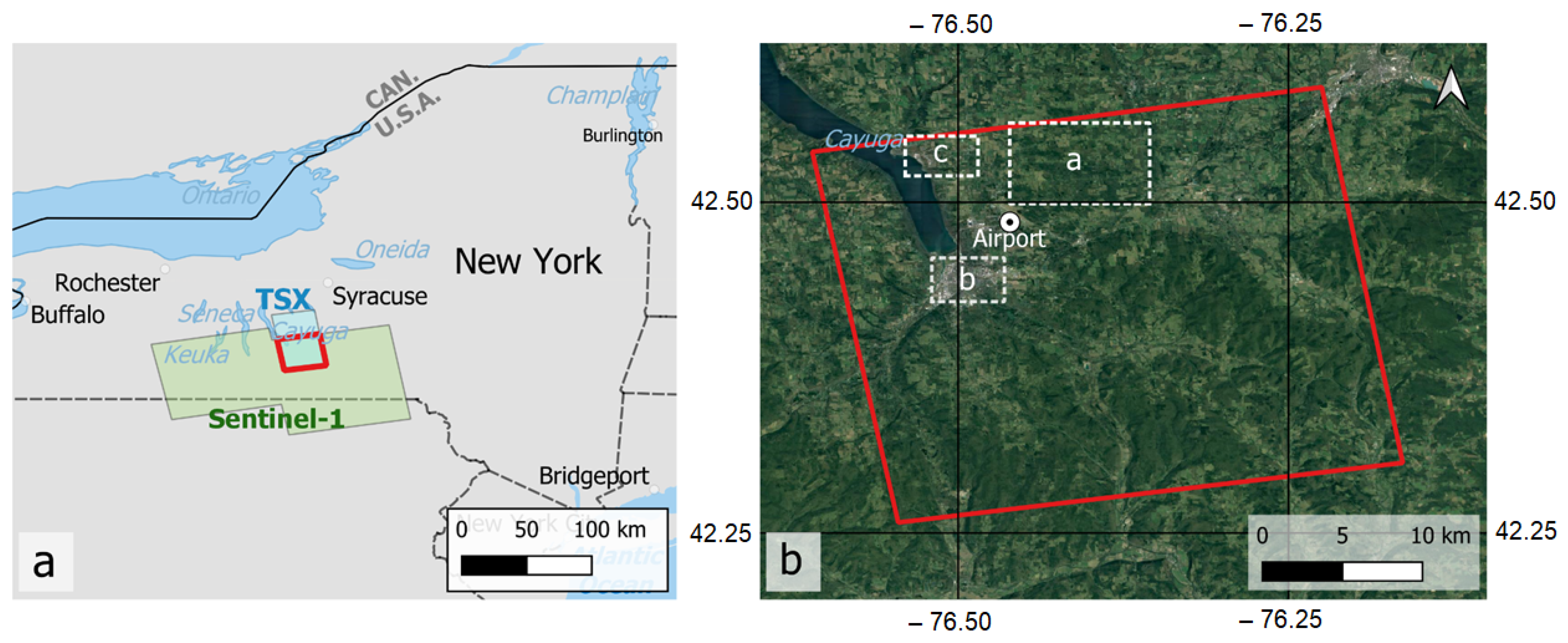
Figure 1.
(a) Overview map of the study area. The S1 and TSX frames are shown in green and blue, respectively. Red indicates the study area covered by both datasets. (b) Target regions within the study area (red (same as in (a)) include a rural, heavily vegetated region (a), the city of Ithaca (b), the Cayuga Salt Mine (c), and the Ithaca airport. Basemap imagery available through Google: imagery @2023 TerraMetrics; map data @2023.
This study aimed to assess the ability of PSI to map displacement rates at the mm/y scale by exploiting the C-band (5.6 cm wavelength) Sentinel-1 (S1; European Space Agency), and the X-band (3.1 cm wavelength) TerraSAR-X and TanDEM-X satellites of the German Space Agency. Below and in the figures, we use “TSX” to refer to data from both the TerraSAR-X and TanDEM-X platforms. We investigated the influence of pixel size, wavelength, and snow-cover changes on the density of PS points identified during PSI analysis and on the accuracy of the measured displacement time series. We utilized the PSI software package StaMPS [
16,
17] for PSI analysis. We evaluated the accuracy of our inferred average displacement rates using ground survey measurements in the Cayuga Salt Mine area [
18,
19].
2. Data and Methodology
The S1 and TSX imagery that we used in this study have different wavelengths, spatial resolutions, and repeat times. Both tracks are acquired while the satellites are travelling in the ascending direction, so the incidence angles are similar (43.4–45.6 degrees for TSX and 36.2–41.7 degrees for S1). The TSX and S1 data cover an overlapping time period from 17 September 2018 to 30 August 2021 (80 acquisitions) and 21 September 2018 to 17 September 2021 (91 acquisitions), respectively.
Figure 1 shows the outline of S1 and TSX tracks that were used in this study. S1 has a minimum repeat visit time of 6 days over selected areas of the world (12 days in the study area when every observation is acquired) and a ground pixel size of 3.9 m (range direction) by 14 m (azimuth direction). TSX has a repeat time of 11 days and a ground range and azimuth resolution of about 2.0 m × 2.0 m. It should be noted that not every possible image is acquired due to satellite downtime and competing observation requests, so there are time-period gaps with more than 11 or 12 days between satellite observations in both the TSX and S1 datasets.
Both the wavelength and pixel size differ significantly between the S1 and TSX datasets, making it difficult to separate the influences of spatial resolution from those of wavelength on data quality. To address this question, we generated spatially averaged TSX data with almost the same pixel size of the S1 data. The downsampling was done using a vector summation of 7 by 2 focused and co-registered SLC pixels in the azimuth and range directions. The spatially averaged TSX (TSX-d) data had the same wavelength as the original TSX data and had almost the same pixel area of the S1 data. Below we compare the results using the TSX-d (-d for downsampled) dataset to those from the TSX and S1 datasets to better understand the separate influences of pixel size and wavelength on the density of PS points and the accuracy of measurement in our study area.
The study area was in Tompkins County, NY, USA, which is covered by a mix of forests, agricultural lands, and relatively small urban/suburban areas and has snowy winters. The phase variability induced by snow cover during winter months can make a pixel less likely to be selected as a PS point [
20]. Snow cover can also negatively impact InSAR time series by introducing both noise and potential biases to the individual interferograms. However, even data acquired when snow is present can potentially contribute useful information to the time series through the generation of shorter-timescale interferograms with less temporal decorrelation. To assess the magnitude of snow cover effects on the resulting time series, we used the three datasets (i.e., TSX, TSX-d, and S1) to generate three snow-free datasets (i.e., TSX-s, TSX-ds, and S1-s) by removing snow-covered images from the data stacks. The snow-covered images were determined using the daily U.S. snowfall and snow depth data provided by the National Centers for Environmental Information (
www.ncdc.noaa.gov, accessed on 15 May 2022 ) and snow depth data from the National Operational Hydrologic Remote Sensing Center (
www.nohrsc.noaa.gov (accessed on 27 May 2022)), including visual inspection of imagery available on each date. A total of 27 out of 80 TSX images and 32 out of 91 S1 images were snow-covered (
Figure 2). This provided an opportunity to assess whether removing wintertime imagery improved or decreased the quality of the resulting inferred average deformation rates.
For each of our six datasets, we examined the density and distribution of PS points and the noise characteristics of the inferred displacement time series in the study area. It should be also noted that in addition to technical and scientific differences, TSX is commercial data while S1 is open and free data.
Figure 2.
Perpendicular baseline in meters vs. date for all data relative to a reference date (red) showing snow-free (black) and snow-covered (blue) dates for TSX (a) and S1 (b).
Figure 2.
Perpendicular baseline in meters vs. date for all data relative to a reference date (red) showing snow-free (black) and snow-covered (blue) dates for TSX (a) and S1 (b).
One role of this study was to inform decisions about the choice of satellite platform and potential costs for tasking of TSX for future deformation-mapping efforts in the study area, the U.S. Northeast, and other similar areas worldwide.
We co-registered the S1 and TSX SLC images and prepared them for PS analysis using the ISCE-2 software [
21]. With ISCE-2, we generated single-reference, full-resolution interferogram stacks. The prepared interferogram stacks were then analyzed using the Stanford Method for Persistent Scatterers (StaMPS) software [
11]. StaMPS identifies pixels that (on average) have the most stable phase values relative to the average phase of their neighbors (often a subset of the most stable neighbors) [
11,
16,
17,
22,
23]. StaMPS removes noisy pixels that are the most sensitive to changes in their scattering properties over time due to factors such as vegetation, soil moisture change, snow, and noise. The resulting set of relatively stable pixels have been shown in other regions to allow for accurate estimates of deformation rates at the mm/year and even sub-mm/year level [
14,
16,
24] when a series of images that is sufficiently well sampled in time is available and the deformation is relatively constant in time.
Our study area included the Cayuga Salt Mine area, which is a useful test site due to the presence of an ongoing ground-based surveying effort [
18,
19]. The salt mine stretches from a region to the north of the city of Ithaca, NY, USA, to underneath the waters of Cayuga Lake. While the area that is not beneath the lake has not been mined since the 1990s, subsidence continues and is observable in the ground-based observations. It is estimated that the subsidence will continue for 200 years or more [
25]. We compared the PS results to vertical elevation differences at 37 benchmarks based on two ground survey campaigns conducted in 2014 and 2021 [
19] and Mark Rowe (personal communication in 2021).
3. Results
Figure 2,
Figure 3,
Figure 4 and
Figure 5 show the PS points extracted using the six datasets over the study area and derived quantities from the PSI time series at those points. As expected, most of the identified PS points were found on stable, artificial structures such as roads and buildings, whereas forests or agricultural fields had fewer PS points. It should be noted that the displacement rates were measured along the LOS between the satellite radar and the ground such that both vertical and horizontal ground movements contributed to the measurement. The subsidence associated with salt mines tends to be dominated by slow collapse of the columns of salt that are left behind during the mining operations, resulting in the eventual closure of the galleries making up the mine and a signal that is dominated by displacements in the vertical direction [
26]. Therefore, we converted the LOS to an inferred vertical displacement rate under the assumption that all ground deformation was vertical. This facilitated comparison between the results of different TSX and S1 datasets and with ground-surveying observations but may have introduced errors if there were significant horizontal displacements present. The average incidence angles of the radar beam are about 44 and 37 degrees, respectively, for the TSX and S1 datasets.
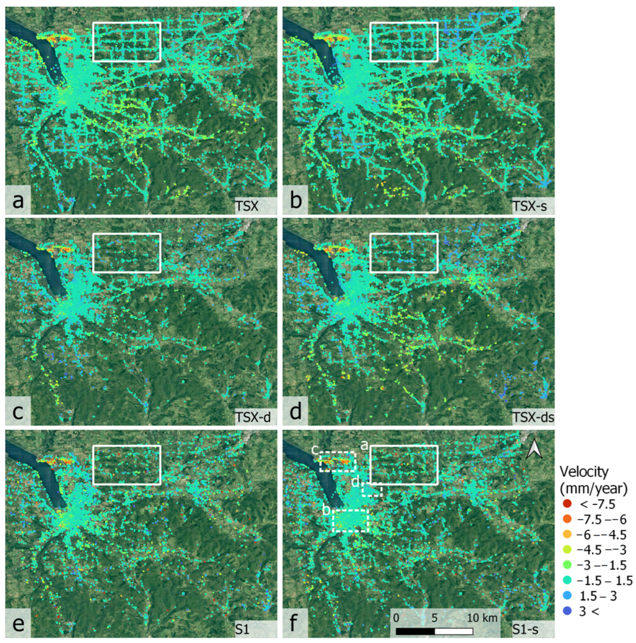
Figure 3 shows the inferred average displacement velocity over the study area (the common area covered by both TSX and S1). The TSX dataset (
Figure 3a) resulted in more PS points than the S1 dataset (
Figure 3e). However, the S1 dataset resulted in more PS points than the spatially averaged TSX dataset (TSX-d) (
Figure 3c). We also showed that the number of PS points increased by 50–60% when we removed snow-covered images (right column of panels in
Figure 3). All six velocity maps in
Figure 3 show that the inferred rates clustered near zero mm/y and had some negative values of up to −7.5 mm/y (indicating an increase in the radar line of sight, which was interpreted as subsidence) and a smaller number of locations with positive values, which would be consistent with ground uplift. All of the six velocity maps show a coherent region of inferred subsidence on the east side of Cayuga Lake with dimensions of about 3 km from east to west and 1 km north–south (box c in
Figure 1b). This area is near Lansing, NY, USA, above an inactive portion of the subsurface salt mine that has been known to be subsiding for decades (see
Section 5 for a comparison of the StaMPS and ground control points).
Figure 3.
PS points extracted by StaMPS using the TSX (
a), TSX-s (
b), TSX-d (
c), TSX-ds (
d), S1 (
e), and S1-s (
f) datasets colored according to the inferred average displacement rate in the vertical direction between 2018 and 2021 with the assumption that all InSAR-observed change was associated with vertical displacements. The labeled white boxes in (
f) are the same as in
Figure 1 but with the addition of (
d) for the airport region and show areas displayed in
Figure 4,
Figure 5 and
Figure 6. Basemap imagery available through Google: imagery @2023 TerraMetrics; map data @2023.
The white box with the solid outline in
Figure 3 (labeled “a” in
Figure 3f) indicates a portion of the study area that was dominated by vegetation and agricultural fields with few roads. The PS points in this area were clustered along the isolated houses and along roads.
Figure 4.
PS density maps extracted using the TSX (
a), TSX-s (
b), TSX-d (
c), TSX-ds (
d), S1 (
e), and S1-s (
f) datasets. The number of PS points over downtown Ithaca (shown as a black box in map f) are given in
Table 1. The area shown in this figure is labeled “b” in
Figure 1. Basemap imagery available through Google: imagery CNES/Airbus, Maxar Technologies, New York GIS, USDA/FPAC/GEO; map data @2023.
Figure 4 shows a heatmap of the density of PS for the six datasets over the city of Ithaca and the surrounding urban setting in Tompkins County, NY, USA. The maps show the number of PS points per square kilometer. It can be seen that downtown Ithaca and Cornell University (~1 km to the northeast of the downtown area), which are dominated by tall buildings, were associated with the densest PS point coverage. It can be seen that the TSX dataset (
Figure 4a) had a higher density of stable PS points than either the S1 dataset or the spatially averaged TSX dataset (TSX-d). The snow-free datasets were associated with a larger number of PS points than the full-stack datasets over the region as a whole or the smaller region shown in
Figure 4.
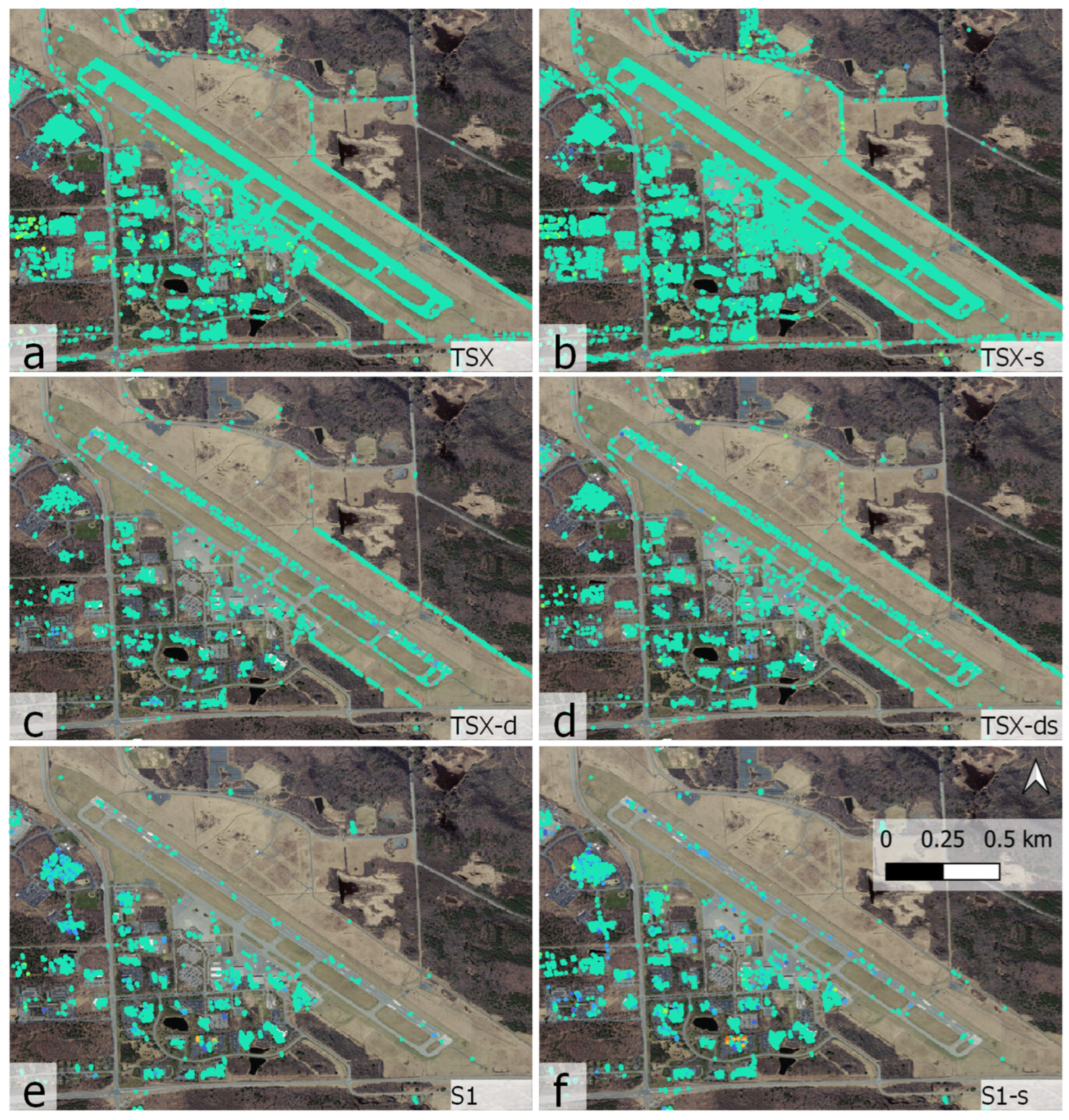
Figure 5.
PS points over the Ithaca Airport. The number of PS points on and along the runway were 2421, 3297, 191, 279, 26, and 49 for TSX (
a), TSX-s (
b), TSX-dv (
c), TSX-ds (
d), S1 (
e), and S1-s (
f), respectively. The colormap is the same as in
Figure 3. Basemap imagery available through Google: imagery CNES/Airbus, Maxar Technologies, New York GIS, USDA/FPAC/GEO; map data @2023.
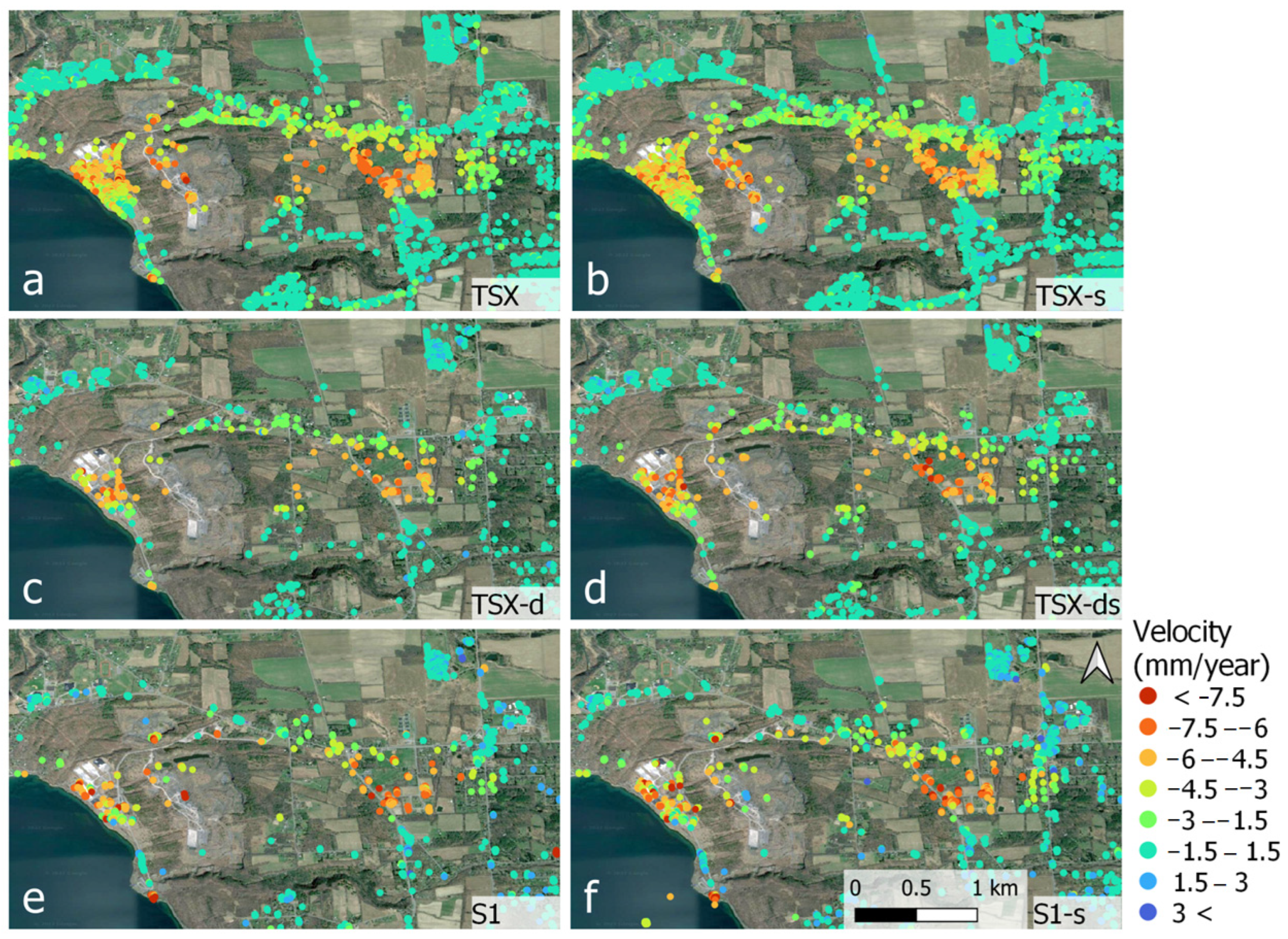
Figure 6.
Displacement rates extracted over Lansing and the Cayuga Salt Mine (CSM) using TSX (
a), TSX-s (
b), TSX-d (
c), TSX-ds (
d), S1 (
e), and S1-s (
f). The displacements were converted from the radar line sight (LOS) to vertical deformations while assuming that all deformations were vertical. The area shown in this figure is labeled “c” in
Figure 1. Basemap imagery available through Google: imagery CNES/Airbus, Maxar Technologies, New York GIS, USDA/FPAC/GEO; map data @2023.
In the vicinity of Ithaca Airport (
Figure 5), we can see a clearer difference in the types of scatterers that were identified as PS in the StaMPS approach. For all datasets, the runway and a series of large warehouses and office buildings to the southwest of the airport were associated with clusters of PS. A key difference can be seen along the fence bounding the fields around the runway—the TSX and TSX-s datasets were associated with a distinct line of PSs along the fencing to the northeast of the runway, while the S1 data was not. The downsampled TSX data did appear to be sensitive to the fencing at a slightly lower level than the full-resolution TSX. In general, the higher density of PSs identified in the TSX-d datasets as compared to the S1 datasets suggested that wavelength is a more important factor than spatial resolution for these types of artificial targets.
4. Discussion
We used six datasets to investigate the influence of wavelength, pixel size, and snow cover on the spatial density, coverage, and reliability of the PS points in Tompkins County, NY, USA, a region where vegetation and snow cover in winter are major obstacles to InSAR analysis. In addition to the original TSX and S1 datasets, we generated spatially averaged TSX observations (TSX-d) with almost the same pixel size as the S1 data. In addition, for each of the three datasets, we generated a snow-free dataset to assess how inclusion of snow-covered dates impacted the resulting time series. In
Table 2, we show ratios of the number of PSs extracted from each dataset type and region to illustrate areas where pixel size, wavelength, or snow cover appeared to be the dominant factors.
4.1. The Influence of Pixel Size
To assess the influence of pixel size, we compared the full-resolution and spatially averaged TSX datasets. The data collected by high-resolution (spatial resolution of a few meters) SAR sensors such as TSX can be critical to the study of objects with small spatial extent. A comparison between the PS numbers and distributions derived from TSX and TSX-d in the study area showed that TSX had about 11 times more PS points compared to the TSX-d data (
Table 2). Note that the pixel size of the TSX dataset was 14 times smaller than the pixel size of the downsampled TSX-d. Therefore, if all of the TSX pixels would have been selected within one of the downsampled TSX-d pixels, we would expect the
ratio to be 14. If each downsampled pixel was dominated by the scattering from a single full-resolution pixel, we would expect the ratio to be near unity. In the “vegetated region” (box a in
Figure 1b), the
ratio was larger than 14 for both the full time series and snow-free time series, suggesting that there was a distinct benefit to the higher-resolution data in that land cover type. Visual inspection of
Figure 5a,c shows that the distribution of PSs differed slightly between the full-resolution and downsampled versions in that fewer of the buildings in the lower left (southeast) of the airport region were associated with stable scatterers.
4.2. The Influence of Wavelength
To assess the influence of wavelength, we compared the spatially averaged X-band TSX data with the C-band S1 observations. The spatially averaged TSX (TSX-d) and S1 datasets had almost the same pixel size—each pixel covered an area of about 56 m
2. The ratio of S1 to TSX-d PS numbers in the study area was about 1.5 overall and differed in different environments (see
Table 2). Considering the fact that wavelength was the main difference between the two datasets, this supported the generally accepted idea that longer microwave wavelengths interact with more stable scatterers [
4]. For instance, over downtown Ithaca (
Figure 4), the ratio was about 1.7. Over the vegetated area in
Figure 3 where PSs were primarily associated with isolated houses, the same ratio was even higher (2.05).
Interestingly, the trends in the density of PS points over Ithaca Tompkins Airport’s runway were the opposite of those in the rest of the area (
Table 2). The ratio of S1 to TSX-d PS numbers near the airport (0.14) was about 15 times smaller than the ratio in the vegetated areas (2.05). The difference can be associated with the fact that the intensity of radar backscattering was related to the ratio of the scatterer dimension to the radar wavelength. The runway along with all of the fencing, pavement, and other artificial structures may have been dominated by smaller scatterers than were found in the more natural terrain.
4.3. The Influence of Snow Cover
To assess the influence of snow cover, we examined the differences between the TSX, TSX-d, and S1 datasets that did or did not include snow-covered dates. Phase changes induced by snow cover during winter months can result in a lower likelihood that a given pixel will have a similar phase to its neighbors over time and be selected as a PS point [
20]. The snow-covered images were identified using the Daily U.S. Snowfall and Snow Depth data provided by the National Centers for Environmental Information (
www.ncdc.noaa.gov, accessed on 15 May 2022). There were a total of 53 snow-free TSX images out of the original dataset of 80 scenes and 59 snow-free S1 images out of the original dataset of 91 scenes.
The ratio of snow-free PS numbers to full-stack PS numbers was different in different environments, but there were more PS points selected from the snow-free datasets than from the full-stack datasets. The smallest differences were found in the urban setting, which showed ratios between the snow-free and full-stack data ranging from 1.22 to 1.27. The largest values (2+) were associated with the vegetated area, which was dominated by vegetation cover and isolated buildings.
Despite the change in the density of PS points, the precision of the deformation rates inferred from the smaller snow-free dataset was not changed significantly, potentially because the summer images tended to also have a larger contribution from tropospheric variability and vegetation changes. For example, the respective average RMSEs of velocity were 4.39, 4.53, 4.12, 4.48, 4.90, and 5.05 mm/year for the TSX, the TSX-s, TSX-d, TSX-ds, S1, S1-s datasets covering the entire study area, which indicated a negligible increase in the RMSE of snow-free velocities.
5. Validation of the Results
Over most of the study region, there is a lack of closely spaced ground-based geodetic observations. However, we were able to evaluate our resulting velocity maps using ground truth measurements over a well-studied underground salt mine in Tompkins County, NY. The part of the mine where measurements were conducted has been inactive for decades but still subsides at a maximum rate of about 1 cm/year ([
19] and Mark Rowe (personal communication in 2021)). As stated above, modeling suggests that subsidence in this area should continue for 200 years or more [
25]. There were benchmark surveying campaigns (leveling) in 1979, 1994, 2004, 2007, 2014, and 2021 ([
19] and Mark Rowe (personal communication in 2021)) that resulted in data that were consistent with a decreasing subsidence rate over time. We compared our velocity maps with the surveying velocity calculated during the most recent time interval (between 2014 and 2021). Because the 2014–2021 time interval extended slightly further back in time than the 2018–2021 InSAR time interval, we expected some slight discrepancy in the rates due to the inclusion of earlier, more rapid deformation in the surveying results. We compare the PSI results to vertical elevation differences at 37 benchmarks among two ground survey campaigns conducted between 2014 and 2021. In 2014, the survey was a part of surface-subsidence monitoring of the Cayuga Salt Mine as reported to the New York State Department of Environmental Conservation. In 2021, the survey was carried out by the Cayuga Lake Environmental Action Network (CLEAN) and conducted by Mark Rowe from Keystone Associates in Binghamton, NY. In the released surveying documents, the subsidence between 1979 and 1994 was roughly twice as high as it was during the time intervals between the more recent measurements in 2004, 2007, and 2014.
All of the six datasets showed a coherent region of inferred subsidence on the east side of Cayuga Lake with dimensions of about 3 km from east to west and 1 km north–south (
Figure 6).
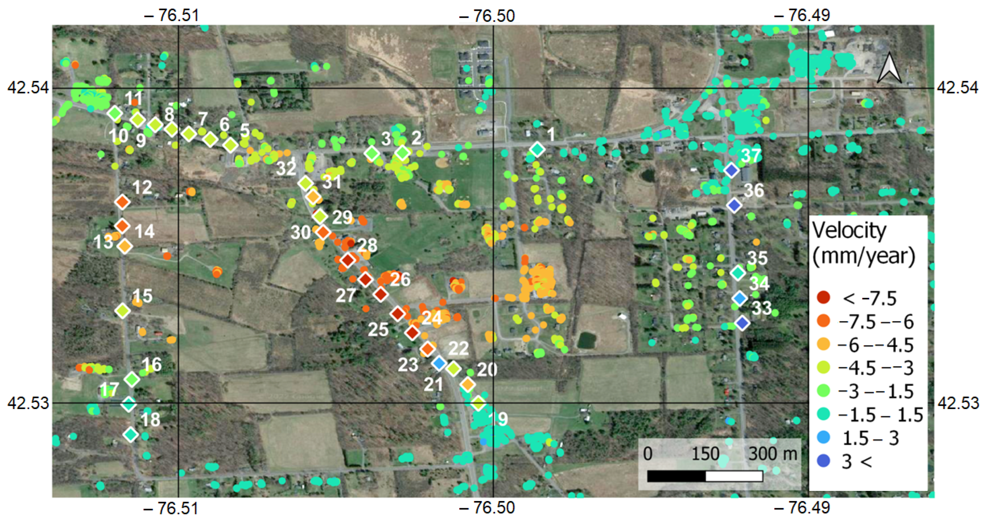
Figure 7 shows a comparison between the ground-based elevation change observations between 2014 and 2021 and the TSX velocity between 2018 and 2021 (
Figure 6). The PS observations were sensitive to both horizontal and vertical components of deformation, while the ground-based observations could (in theory) measure both the horizontal and vertical components separately (to different levels of accuracy). Some of the observed discrepancy may have been due to the contribution of horizontal displacement to the PS observations, which we implicitly assumed to be zero when we converted the PS displacement rates to the vertical direction.
As can be seen in
Figure 7, the displacements between 2014 and 2021 at five of the ground control points (points 33–37) were positive (uplift). It is unlikely that any processes associated with the inactive mine would result in uplift, so the inferred uplift was potentially due to issues with the reference point used in surveying or seasonal signals associated with groundwater loading or poroelastic responses. Below, we focus on sites to the west where the ground control points indicated ongoing subsidence.
For each GCP, the average PSI velocity within a radius of 50 m around the GCP station was calculated and compared to the 2014–2021 displacement rate at the station. A distance of 50 m was chosen because it was similar to the spacing between GCP points along the main roads seen in
Figure 7 and because the displacement rates associated with the mine varied over a spatial scale several times larger than that distance. For the TSX dataset shown in
Figure 7, the number of points associated with each GCP ranged from 0 to 62 and had a mean value of 10 TSX PSI values in the vicinity of each GCP. For the GCP points that were spaced most closely to each other, there was some overlap in the 50 m window (e.g., points 2–11 in the north of
Figure 7), but there was also little variability among the PSI velocity values across that region. The RMSE of differences between the average PSI velocities and 2014–2021 displacement rates at all GCP stations were 1.29, 1.35, 1.49, 1.41, 1.80, and 1.81 mm/year for the TSX, TSX-s, TSX-d, TSX-ds, S1, and S1-s datasets, respectively. It should be noted that in the calculations, we excluded GCP stations with positive (uplift) rates.
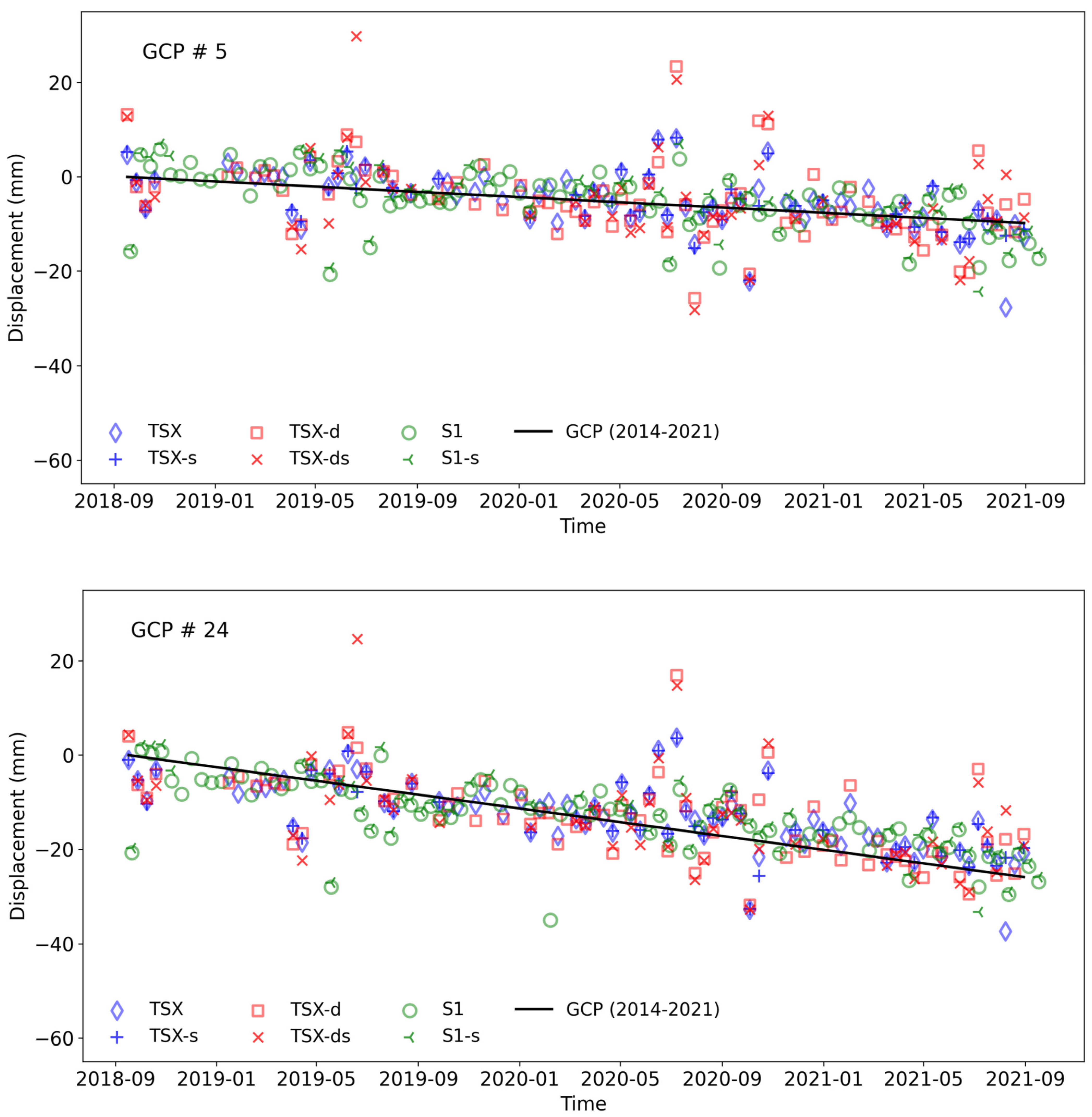
Figure 8 illustrates a comparison between PSI-inferred deformation time series and ground surveying at two surveying stations (GCP #5 and GCP #24). The plots show a good agreement between the InSAR results and the surveying-based velocity.
In addition to evaluating the PSI results with survey measurements, we compared the deformation time series from different datasets. It is shown in
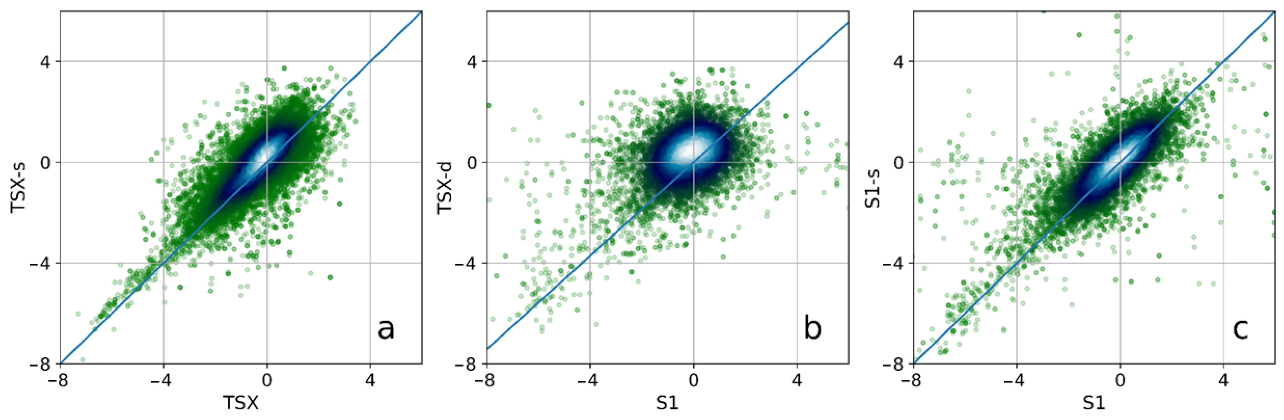
Figure 5 that the TSX and TSX-s datasets (panels a and b) had a higher density of stable PS points and less scatter among the inferred rate at these points than can be seen in the S1 and S1-s datasets (panels c and d). To compare the results between different satellites, we spatially averaged all velocity maps onto a common 100 m grid covering the entire region. We then generated scatter plots between the resampled datasets (
Figure 9). An LOS ratio line was also mapped on the plots to illustrate the effect of viewing geometry (1:1 in the case of a comparison between a given dataset and its snow-free equivalent). The TSX and S1 velocities were correlated with their snow-free velocities, but the S1 datasets were more scattered compared to the TSX datasets. Many pixels with more negative values were common to both (lower-left quadrant of
Figure 9b), but there were also some large and small S1 values that were associated with near-zero rates in the TSX-d dataset. The high correlation between the full-stack and snow-free datasets indicated that exclusion of the datasets impacted by snow and rain did not appear to result in a bias in the magnitude of the inferred average displacement rate, although a slight positive bias may have been present for TSX-s vs. TSX.
6. Conclusions
We used X-band (TerraSAR-X and TanDEM-X) and C-band (Sentinel-1) satellite data and applied persistent scatterer InSAR (PSI) analysis using the StaMPS software package for data covering a region in Tompkins County between 2018 and 2021. We generated six datasets to investigate the influence of wavelength, pixel size, and snow cover on the density and accuracy of the PS points in the study area, in which vegetation and snow cover in winter are major obstacles to InSAR analysis. We generated spatially averaged TSX data with almost the same pixel size of the S1 data to assess and separate the influences of wavelength and pixel size on the density and reliability of PS points. In addition, for each of the three datasets, a snow-free dataset was generated to assess the influence of snow cover on the results.
A comparison between the TSX and TSX-d results showed that the influence of spatial resolution on the density of PS points was stronger in the vegetated areas compared to the urban area. This might have indicated that “non-stable” pixels within a spatial averaging window in the vegetated areas were more likely to lead a spatially averaged pixel to not be selected as a PS pixel. In the urban areas, such influences were relatively small.
When we attempted to correct for pixel size by comparing the TSX-d and S1 data, we found that the longer-wavelength data resulted in more PS points over most of the study area. The exception was in the vicinity of the airport, where smaller scatterers associated with artificial structures resulted in more PSs for the TSX-d observations relative to the S1 observations.
We compared our PSI results to an example in the Lansing area associated with an underground salt mine where rates of subsidence of up to 10 mm/y have been measured using ground surveys. To evaluate the accuracy of our results, we compared the measured displacement rates from the different satellites to each other and with the rates observed at the ground control points between 2014 and 2021. Our results also showed that removing TSX and S1 images on the days of snow did increase the number of persistent scatterers but did not improve the precision of the deformation measurements. The S1 and TSX rate measurements were consistent with each other, particularly within the region of subsidence. However, TSX provided better spatial sampling because there were more persistent scatterers identified from within the TSX imagery. The comparison with ground control points supported our conclusion that the TSX data were more accurate (root-mean-square difference of 1.29 mm/y) compared to the S1 data (root-mean-square difference of 1.80 mm/y). For researchers attempting to determine whether the additional cost associated with tasking and purchasing TSX data is justified, the key distinction may be the spatial coverage (particularly for signals of spatial scales close to the larger S1 pixel sizes) or the improvement in accuracy, depending on their goals.


