
Small Recreational Boat Detection Using Sentinel-1 Data for the Monitoring of Recreational Ecosystem Services


Abstract
:1. Introduction
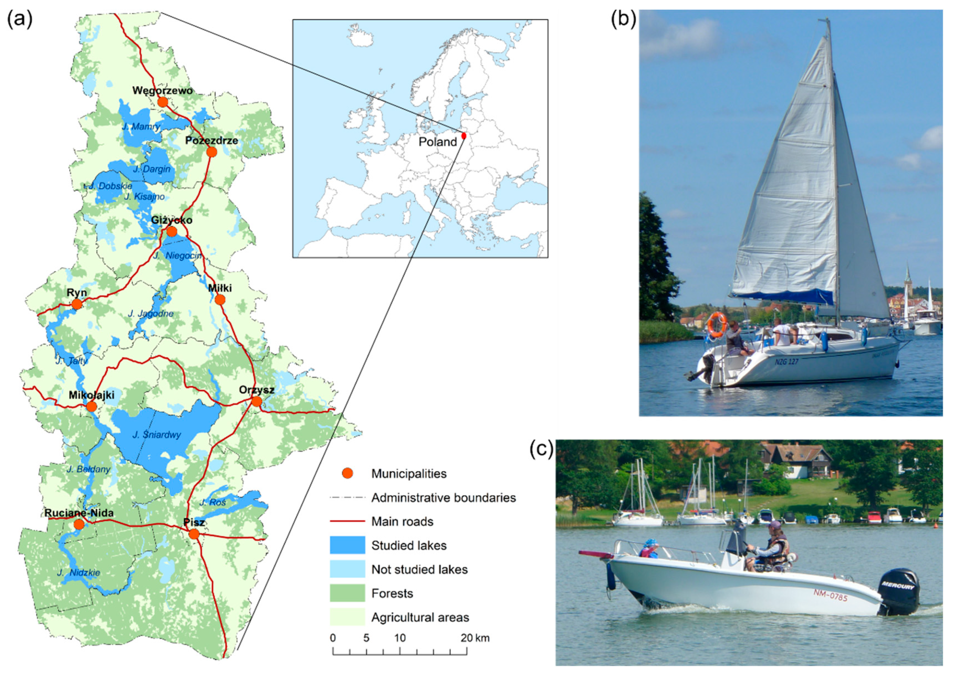
2. Study Area
2.1. Characteristics of the Study Area
- Moraine-dammed lakes are large (minimum distance between shores greater than 1.5 km), with a relatively regular shape. They are mostly surrounded by flat, arable land and meadows. The annual mean wind speed over these lakes varies from 5.49 m/s (the smallest) to 6.06 m/s (the largest). It should also be noted that the mean wind speed is higher in the northern part of the study area. Western winds dominate, followed by southern winds [39].
- Ribbon lakes are very long and narrow. They are surrounded by high banks and forests; the mean wind speed over these lakes varies from 4.44 to 5.45 m/s.
- Kettle lakes are small and round; these lakes are very seldom used for sailing.
2.2. Characteristics of Recreational Boats in the Area
3. Materials and Methods
3.1. Materials
- The first consisted of data collected in 2014 and 2015 through structured field observations [14]. All recreational water activities (sailing boats, motorboats, etc.) that took place in viewsheds were described. These observations were used to obtain a model of the spatial distribution of boats [41]. The data derived from field observations can be used for validation at the lake level, as it has a low spatial resolution.
- The second consisted of 769 reference points, collected via a visual interpretation of images captured over seven lakes. These lakes were selected based on their shape (four moraine-dammed lakes and three ribbon lakes) and the intensity of use. Images from 14 dates were randomly selected to cover different weather conditions. Finally, 325 points representing boats, and 444 points representing water were collected (Table 1).
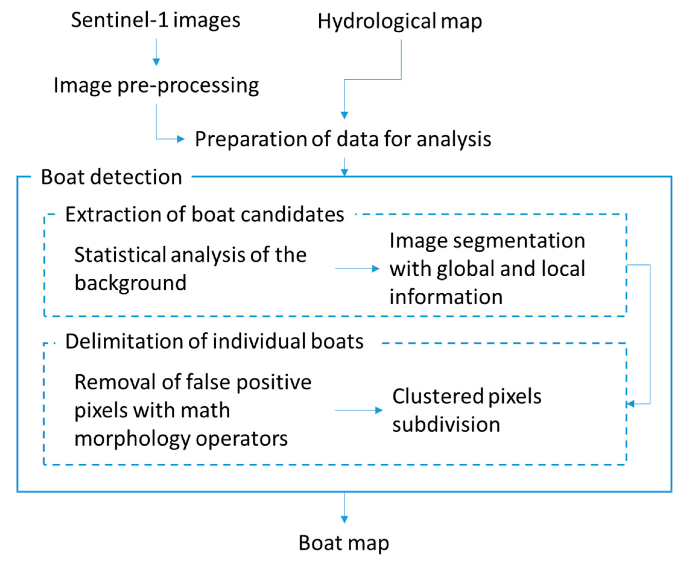
3.2. Method Used to Detect Recreational Boats
3.2.1. Image Preprocessing and Data Preparation
3.2.2. Recreational Boat Detection
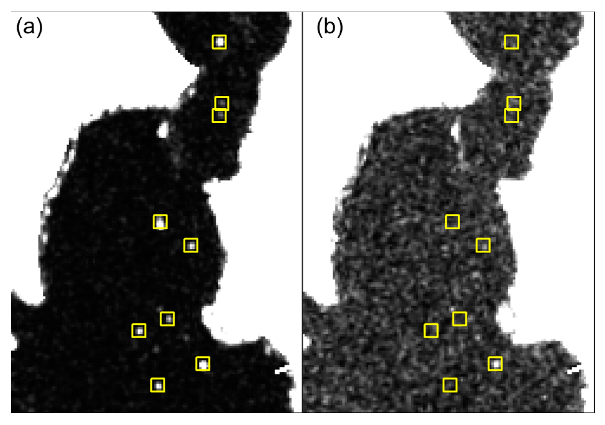
- Lakes are relatively small; the vast majority in our study area are less than 5 km2.
- Lakes have an irregular shape; hence, the local background, defined as a square tile, may contain multiple pixels that correspond to onshore objects with relatively high backscatter (buildings and forests).
- Recreational boats are small; the power of backscatter received from them is lower than that received from onshore objects.
3.2.3. Validation
- checking individual boat detections based on reference points for selected images and the calculation of the error matrix;
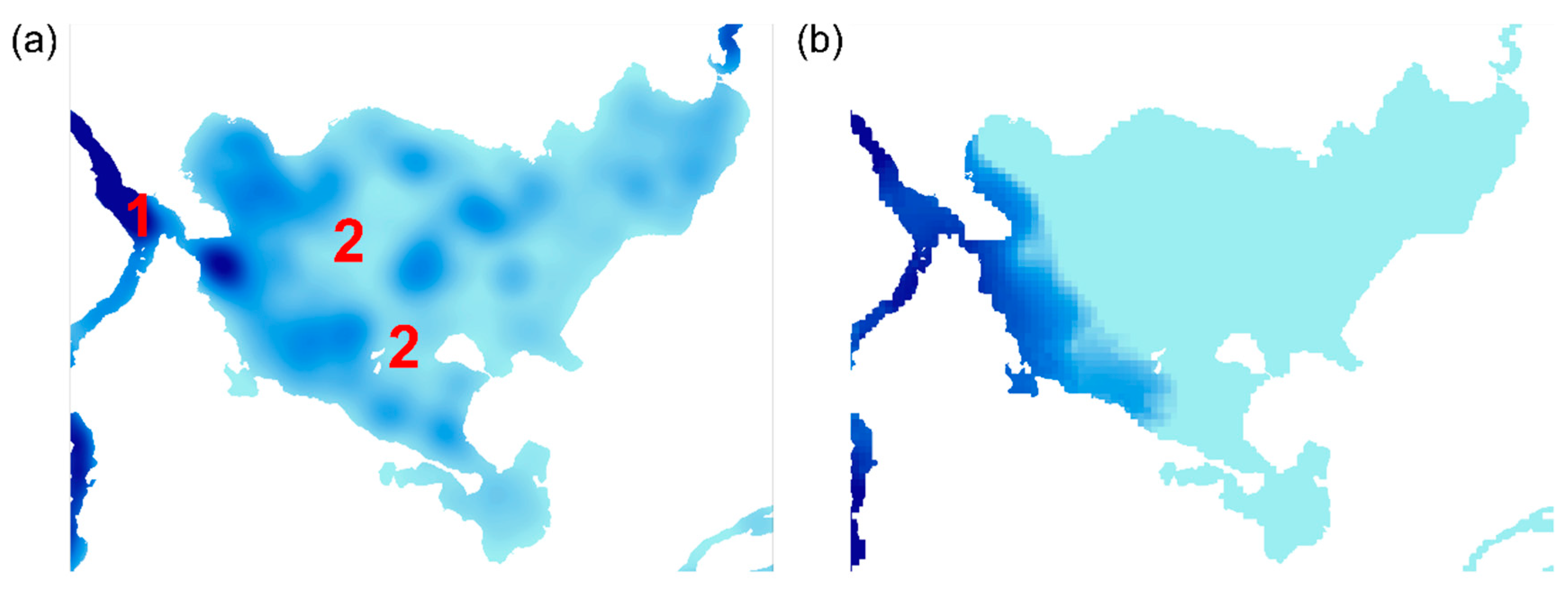
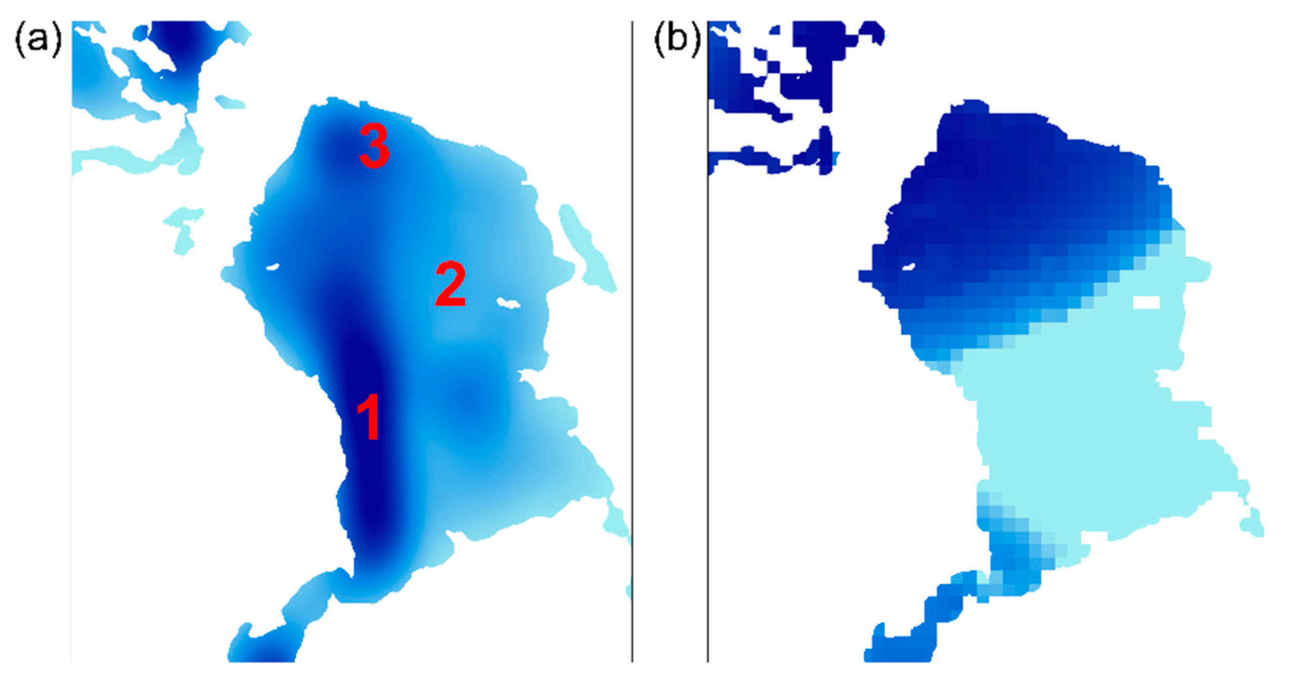
- comparing the spatial distribution of all boats detected in 2015 to a distribution model derived from field observations;
- comparing our algorithm’s results with results obtained using the object detection algorithm implemented in SNAP software [31].
4. Results
4.1. Classification Accuracy
4.1.1. Evaluation of the Boat Detection Method
4.1.2. Evaluation Results as a Function of the Classification Step
4.2. Spatial Distribution of Recreational Boats
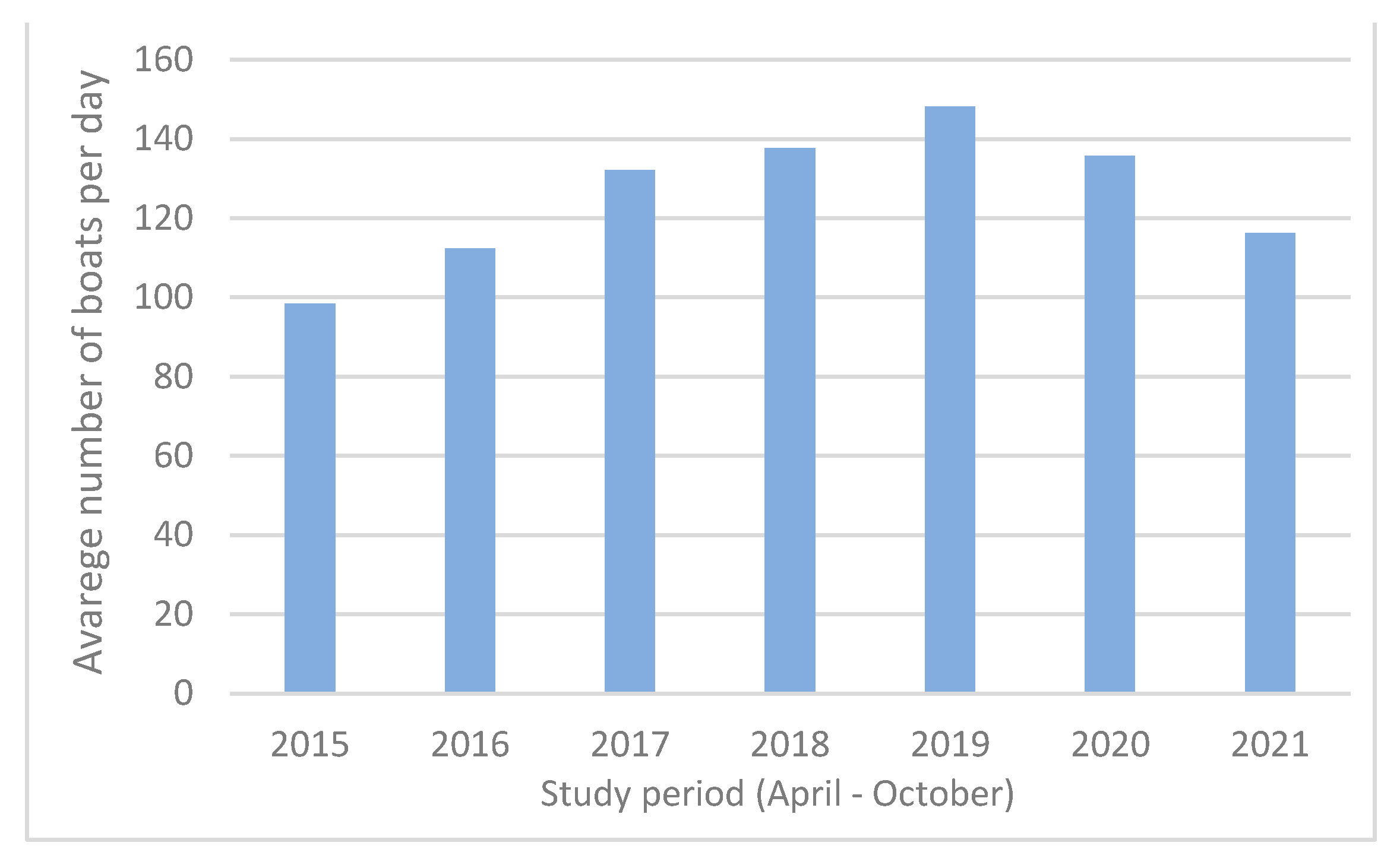
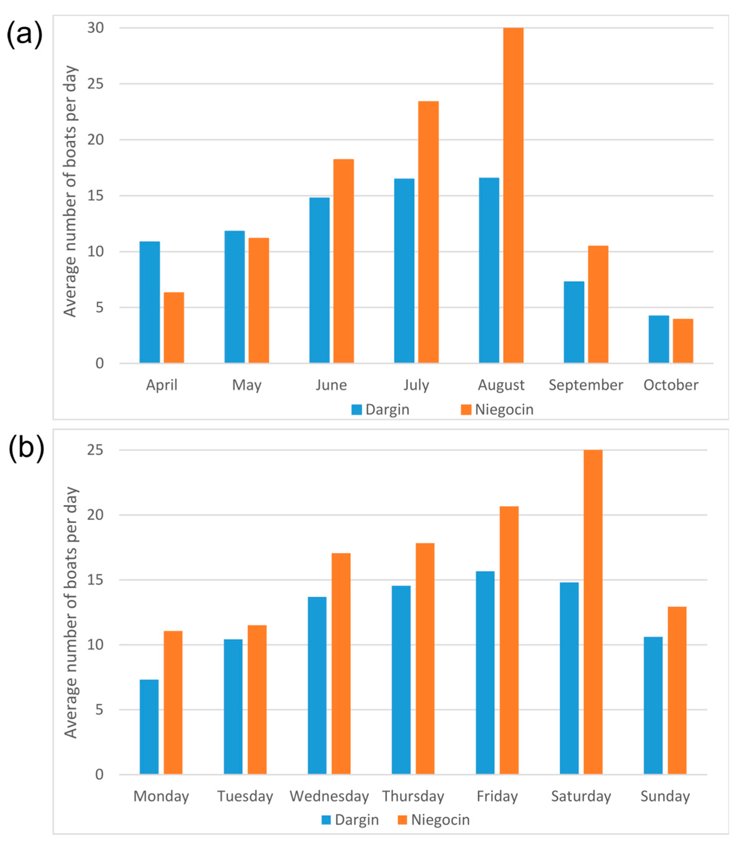
4.3. Temporal Distribution of Recreational Boats
5. Discussion
6. Conclusions
Author Contributions
Funding
Data Availability Statement
Conflicts of Interest
References
- Hall, C.M.; Härkönen, T. (Eds.) Lake Tourism: An Integrated Approach to Lacustrine Tourism Systems; Channel View Publications: Clevedon, UK, 2006; Volume 32, 235p. [Google Scholar]
- Hall, C.M. Trends in ocean and coastal tourism: The end of the last frontier? Ocean Coast. Manag. 2001, 44, 601–618. [Google Scholar] [CrossRef]
- McCole, D.; Joppe, M. The search for meaningful tourism indicators: The case of the international upper great lakes study. J. Policy Res. Tour. Leis. Events 2014, 6, 248–263. [Google Scholar] [CrossRef]
- Venturini, S.; Massa, F.; Castellano, M.; Fanciulli, G.; Povero, P. Recreational boating in the Portofino Marine Protected Area (MPA), Italy: Characterization and analysis in the last decade (2006–2016) and some considerations on management. Mar. Policy 2021, 127, 103178. [Google Scholar] [CrossRef]
- Landré, M. Analyzing yachting patterns in the Biesbosch National Park using GIS technology. Technovation 2009, 29, 602–610. [Google Scholar] [CrossRef]
- Leon, L.M.; Warnken, J. Copper and sewage inputs from recreational vessels at popular anchor sites in a semi-enclosed Bay (Qld, Australia): Estimates of potential annual loads. Mar. Pollut. Bull. 2008, 57, 838–845. [Google Scholar] [CrossRef]
- Hansen, J.P.; Sundblad, G.; Bergström, U.; Austin, Å.N.; Donadi, S.; Eriksson, B.K.; Eklöf, J.S. Recreational boating degrades vegetation important for fish recruitment. Ambio 2019, 48, 539–551. [Google Scholar] [CrossRef] [Green Version]
- Balaguer, P.; Diedrich, A.; Sardá, R.; Fuster, M.; Cañellas, B.; Tintoré, J. Spatial analysis of recreational boating as a first key step for marine spatial planning in Mallorca (Balearic Islands, Spain). Ocean. Coast. Manag. 2011, 54, 241–249. [Google Scholar] [CrossRef]
- Skłodowski, J.; Sater, J.; Strzyżewski, T. Presja turystyki wodnej w ekotonach leśno− jeziornych na przykładzie jeziora Bełdany. Sylwan 2006, 10, 65–71. [Google Scholar]
- Rako, N.; Fortuna, C.M.; Holcer, D.; Mackelworth, P.; Nimak-Wood, M.; Pleslić, G.; Picciulin, M. Leisure boating noise as a trigger for the displacement of the bottlenose dolphins of the Cres–Lošinj archipelago (northern Adriatic Sea, Croatia). Mar. Pollut. Bull. 2013, 68, 77–84. [Google Scholar] [CrossRef]
- Tseng, Y.P.; Kyle, G.T.; Shafer, C.S.; Graefe, A.R.; Bradle, T.A.; Schuett, M.A. Exploring the Crowding–Satisfaction Relationship in Recreational Boating. Environ. Manag. 2009, 43, 496–507. [Google Scholar] [CrossRef]
- Riungu, G.K.; Hallo, J.C.; Backman, K.F.; Brownlee, M.; Beeco, J.A.; Larson, L.R. Water-based recreation management: A normative approach to reviewing boating thresholds. Lake Reserv. Manag. 2020, 36, 139–154. [Google Scholar] [CrossRef]
- Ashton, P.G.; Chubb, M. A preliminary study for evaluating the capacity of waters for recreational boating 1. JAWRA J. Am. Water Resour. Assoc. 1972, 8, 571–577. [Google Scholar] [CrossRef]
- Kulczyk, S.; Woźniak, E.; Derek, M.; Kowalczyk, M. Pomiar marszrutowy jako narzędzie monitoringu aktywności turystycznej. Przykład Wielkich Jezior Mazurskich. Probl. Ekol. Kraj. 2015, 29, 111–120. [Google Scholar]
- Ryan, K.L.; Hall, N.G.; Lai, E.K.; Smallwood, C.B.; Tate, A.; Taylor, S.M.; Wise, B.S. Statewide Survey of Boat-Based Recreational Fishing in Western Australia 2017/18. 2019. Available online: https://www.fish.wa.gov.au/Documents/research_reports/frr297.pdf (accessed on 2 March 2023).
- Gray, D.L.; Canessa, R.; Rollins, R.; Keller, C.P.; Dearden, P. Incorporating recreational users into marine protected area planning: A study of recreational boating in British Columbia, Canada. Environ. Manag. 2010, 46, 167–180. [Google Scholar] [CrossRef]
- Afrifa-Yamoah, E.; Taylor, S.M.; Mueller, U. Modelling climatic and temporal influences on boating traffic with relevance to digital camera monitoring of recreational fisheries. Ocean. Coast. Manag. 2021, 215, 105947. [Google Scholar] [CrossRef]
- Pelot, R.; Wu, Y. Classification of recreational boat types based on trajectory patterns. Pattern Recognit. Lett. 2007, 28, 1987–1994. [Google Scholar] [CrossRef]
- Van den Bemt, V.; Doornbos, J.; Meijering, L.B.; Plegt, M.; Theunissen, N. Teaching ethics when working with geocoded data: A novel experiential learning approach. J. Geogr. High. Educ. 2018, 42, 293–310. [Google Scholar] [CrossRef] [Green Version]
- Meijles, E.W.; Daams, M.N.; Ens, B.J.; Heslinga, J.H.; Sijtsma, F.J. Tracked to protect-Spatiotemporal dynamics of recreational boating in sensitive marine natural areas. Appl. Geogr. 2021, 130, 102441. [Google Scholar] [CrossRef]
- Vachon, P.W.; Campbell, J.W.M.; Bjerkelund, C.A.; Dobson, F.W.; Rey, M.T. Ship Detection by the RADARSAT SAR: Validation of Detection Model Predictions. Can. J. Remote Sens. 1997, 23, 48–59. [Google Scholar] [CrossRef]
- Touzi, R.; Charbonneau, F.J.; Hawkins, R.K.; Vachon, P.W. Ship detection and characterization using polarimetric SAR. Can. J. Remote Sens. 2004, 30, 552–559. [Google Scholar] [CrossRef]
- Pelich, R.; Longépé, N.; Hajduch, G.; Mercier, G. Performance evaluation of Sentinel-1 data in SAR ship detection. In Proceedings of the IEEE International Geoscience and Remote Sensing Symposium (IGARSS), Milan, Italy, 26–31 July 2015. [Google Scholar]
- Tings, B.; Bentes, C.; Velotto, D.; Voinov, S. Modelling ship detectability depending on TerraSAR-X-derived metocean parameters. CEAS Space J. 2019, 11, 81–94. [Google Scholar] [CrossRef] [Green Version]
- Shirvany, R.; Tourneret, J.Y. Ship and Oil-Spill Detection Using the Degree of Polarization in Linear and Hybrid/Compact Dual-Pol SAR. IEEE J. Sel. Top. Appl. Earth Obs. Remote Sens. 2012, 5, 885–892. [Google Scholar] [CrossRef] [Green Version]
- Trello, M.; Lopez-Martinez, C.; Mallorqui, J.J. A Novel Algorithm for Ship Detection in SAR Imagery Based on the Wavelet Transform. IEEE Geosci. Remote Sens. Lett. 2005, 2, 201–205. [Google Scholar] [CrossRef]
- Robey, F.C.; Fuhrmann, D.R.; Kelly, E.J.; Nitzberg, R. A Cfar Adaptive Matched-Filter Detector. IEEE Trans. Aerosp. Electron. Syst. 1992, 28, 208–216. [Google Scholar] [CrossRef] [Green Version]
- Gao, G. A Parzen-Window-Kernel-Based CFAR algorithm for ship detection in SAR Images. IEEE Geosci.Remote Sens. Lett. 2011, 8, 557–561. [Google Scholar] [CrossRef]
- Greidanus, H.; Alvarez, M.; Santamaria, C.; Thoorens, F.X. The SUMO Ship Detector Algorithm for Satellite Radar Images. Remote Sens. 2017, 9, 246. [Google Scholar] [CrossRef] [Green Version]
- Gao, G.; Gao, S.; He, J.; Li, G. Adaptive Ship Detection in Hybrid-Polarimetric SAR Images Based on the Power-Entropy Decomposition. IEEE Trans. Geosci. Remote Sens. 2018, 56, 5394–5407. [Google Scholar] [CrossRef]
- Crisp, D.J. The State-of-the-Art in Ship Detection in Synthetic Apreture Radar Imagery; DSTO-RR-0272; Defence Science and Technology Organisation Salisbury (Australia) Info Sciences Lab.: Edinburgh, Australia, 2004. [Google Scholar]
- Wei, S.; Zeng, X.; Qu, Q.; Wang, M.; Su, H.; Shi, J. HRSID: A High-Resolution SAR Images Dataset for Ship Detection and Instance Segmentation. IEEE Access 2020, 8, 120234–120254. [Google Scholar] [CrossRef]
- Zhang, T.; Zhang, X.; Ke, X. Quad-FPN: A Novel Quad Feature Pyramid Network for SAR Ship Detection. Remote Sens. 2021, 13, 2771. [Google Scholar] [CrossRef]
- Sun, Z.; Meng, C.; Cheng, J.; Zhang, Z.; Chang, S. A Multi-Scale Feature Pyramid Network for Detection and Instance Segmentation of Marine Ships in SAR Images. Remote Sens. 2022, 14, 6312. [Google Scholar] [CrossRef]
- Grosso, E.; Guida, R. A New Automated Ship Wake Detector for Small and Go-Fast Ships in Sentinel-1 Imagery. Remote Sens. 2022, 14, 6223. [Google Scholar] [CrossRef]
- Wang, C.; Su, W.; Gu, H. Two-stage ship detection in synthetic aperture radar images based on attention mechanism and extended pooling. J. Appl. Remote Sens. 2020, 14, 044522. [Google Scholar] [CrossRef]
- Zhang, T.; Quan, S.; Yang, Z.; Guo, W.; Zhang, Z.; Gan, H. A Two-Stage Method for Ship Detection Using PolSAR Image. IEEE Trans. Geosci. Remote Sens. 2022, 60, 5236918. [Google Scholar] [CrossRef]
- Kulczyk, S.; Derek, M.; Woźniak, E. Zagospodarowanie turystyczne strefy brzegowej jezior na potrzeby żeglarstwa-przykład wielkich jezior mazurskich. Prace Studia Geogr. 2016, 61, 27–49. [Google Scholar]
- Available online: https://globalwindatlas.info/en/ (accessed on 1 November 2022).
- Available online: https://www.geoportal.gov.pl/dane/baza-danych-obiektow-topograficznych-bdot (accessed on 1 November 2022).
- Kulczyk, S.; Woźniak, E.; Derek, M. Landscape, facilities and visitors: An integrated model of Recreational Ecosystem Services. Ecosyst. Serv. 2018, 31, 491–501. [Google Scholar] [CrossRef]
- Serra, J. Introduction to mathematical morphology. Comput. Vis. Graph. Image Process. 1986, 35, 283–300. [Google Scholar] [CrossRef]
- Congalton, R.G. A Review of Assessing the Accuracy of Classifications of Remotely Sensed Data. Remote Sens. Environ. 1991, 37, 35–46. [Google Scholar] [CrossRef]


| Lake | Type of Lake | Date | Incident Angle | Wind Speed [m/s] | Number of Reference Points | |
|---|---|---|---|---|---|---|
| Boats | Water | |||||
| Bełdany | Ribbon | 11/08/2018 | 38.2–38.5 | 2 | 6 | 43 |
| Bełdany | Ribbon | 20/06/2021 | 38.2–38.5 | 3 | 22 | 25 |
| Dargin | Moraine-dammed | 26/04/2019 | 39.2–39.6 | 3 | 13 | 25 |
| Dargin | Moraine-dammed | 19/07/2020 | 39.2–39.6 | 1 | 42 | 44 |
| Kisajno | Moraine-dammed | 05/08/2018 | 39.1–39.4 | 1 | 14 | 15 |
| Kisajno | Moraine-dammed | 13/08/2019 | 39.1–39.4 | 3 | 15 | 21 |
| Mikołajskie | Ribbon | 04/08/2017 | 38.4–38.6 | 2 | 22 | 25 |
| Mikołajskie | Ribbon | 31/07/2020 | 38.4–38.6 | 3 | 10 | 10 |
| Niegocin | Moraine-dammed | 15/08/2015 | 39.1–39.6 | 2 | 42 | 51 |
| Niegocin | Moraine-dammed | 20/07/2021 | 39.1–39.6 | 3 | 22 | 25 |
| Roś | Ribbon | 29/06/2016 | 39.2–39.8 | 3 | 15 | 17 |
| Roś | Ribbon | 16/05/2021 | 39.2–39.8 | 4 | 29 | 35 |
| Śniardwy | Moraine-dammed | 17/07/2017 | 38.6–39.6 | 3 | 6 | 7 |
| Śniardwy | Moraine-dammed | 08/05/2020 | 38.6–39.6 | 1 | 67 | 101 |
| Sum | 325 | 444 | ||||
| All Reference Datasets | ||
|---|---|---|
| Boat | Water | |
| Boat | 281 | 47 |
| Water | 44 | 397 |
| Producer’s accuracy | 0.86 | 0.89 |
| User’s accuracy | 0.86 | 0.9 |
| F1 score | 0.86 | 0.9 |
| Overall accuracy | 88.17 | |
| Kappa | 0.76 | |
| Ribbon Lakes | Moraine-Dammed Lakes | |||
|---|---|---|---|---|
| Boat | Water | Boat | Water | |
| Boat | 90 | 8 | 191 | 39 |
| Water | 14 | 147 | 30 | 250 |
| Producer’s accuracy | 0.87 | 0.95 | 0.86 | 0.87 |
| User’s accuracy | 0.92 | 0.91 | 0.83 | 0.89 |
| F1 score | 0.89 | 0.93 | 0.85 | 0.88 |
| Overall accuracy | 91.51 | 86.47 | ||
| Kappa | 0.82 | 0.73 | ||
| Erode Filter | Multi-Object Division | Dilation Filter | Producer’s Accuracy | User’s Accuracy | F1 | Overall Accuracy | Kappa |
|---|---|---|---|---|---|---|---|
| no | no | no | 0.74 | 0.76 | 0.75 | 79.71 | 0.58 |
| no | yes | no | 0.78 | 0.65 | 0.71 | 76.00 | 0.51 |
| yes | no | no | 0.72 | 0.89 | 0.79 | 83.78 | 0.66 |
| yes | yes | no | 0.76 | 0.88 | 0.81 | 85.27 | 0.69 |
| yes | no | yes | 0.74 | 0.91 | 0.82 | 85.43 | 0.70 |
| yes | yes | yes | 0.86 | 0.86 | 0.86 | 88.17 | 0.76 |
| 2015 | 2016 | 2017 | 2018 | 2019 | 2020 | 2021 | |
|---|---|---|---|---|---|---|---|
| 2015 | 1.00 | 0.47 | 0.59 | 0.58 | 0.47 | 0.55 | 0.55 |
| 2016 | 1.00 | 0.60 | 0.62 | 0.54 | 0.73 | 0.63 | |
| 2017 | 1.00 | 0.76 | 0.80 | 0.84 | 0.82 | ||
| 2018 | 1.00 | 0.67 | 0.79 | 0.75 | |||
| 2019 | 1.00 | 0.76 | 0.73 | ||||
| 2020 | 1.00 | 0.85 | |||||
| 2021 | 1.00 |
Disclaimer/Publisher’s Note: The statements, opinions and data contained in all publications are solely those of the individual author(s) and contributor(s) and not of MDPI and/or the editor(s). MDPI and/or the editor(s) disclaim responsibility for any injury to people or property resulting from any ideas, methods, instructions or products referred to in the content. |
© 2023 by the authors. Licensee MDPI, Basel, Switzerland. This article is an open access article distributed under the terms and conditions of the Creative Commons Attribution (CC BY) license (https://creativecommons.org/licenses/by/4.0/).
Share and Cite
Ruciński, M.; Woźniak, E.; Kulczyk, S.; Derek, M. Small Recreational Boat Detection Using Sentinel-1 Data for the Monitoring of Recreational Ecosystem Services. Remote Sens. 2023, 15, 1807. https://doi.org/10.3390/rs15071807
Ruciński M, Woźniak E, Kulczyk S, Derek M. Small Recreational Boat Detection Using Sentinel-1 Data for the Monitoring of Recreational Ecosystem Services. Remote Sensing. 2023; 15(7):1807. https://doi.org/10.3390/rs15071807
Chicago/Turabian StyleRuciński, Marek, Edyta Woźniak, Sylwia Kulczyk, and Marta Derek. 2023. "Small Recreational Boat Detection Using Sentinel-1 Data for the Monitoring of Recreational Ecosystem Services" Remote Sensing 15, no. 7: 1807. https://doi.org/10.3390/rs15071807