
New Remote Sensing Data on the Potential Presence of Permafrost in the Deosai Plateau in the Himalayan Portion of Pakistan

Abstract
:1. Introduction
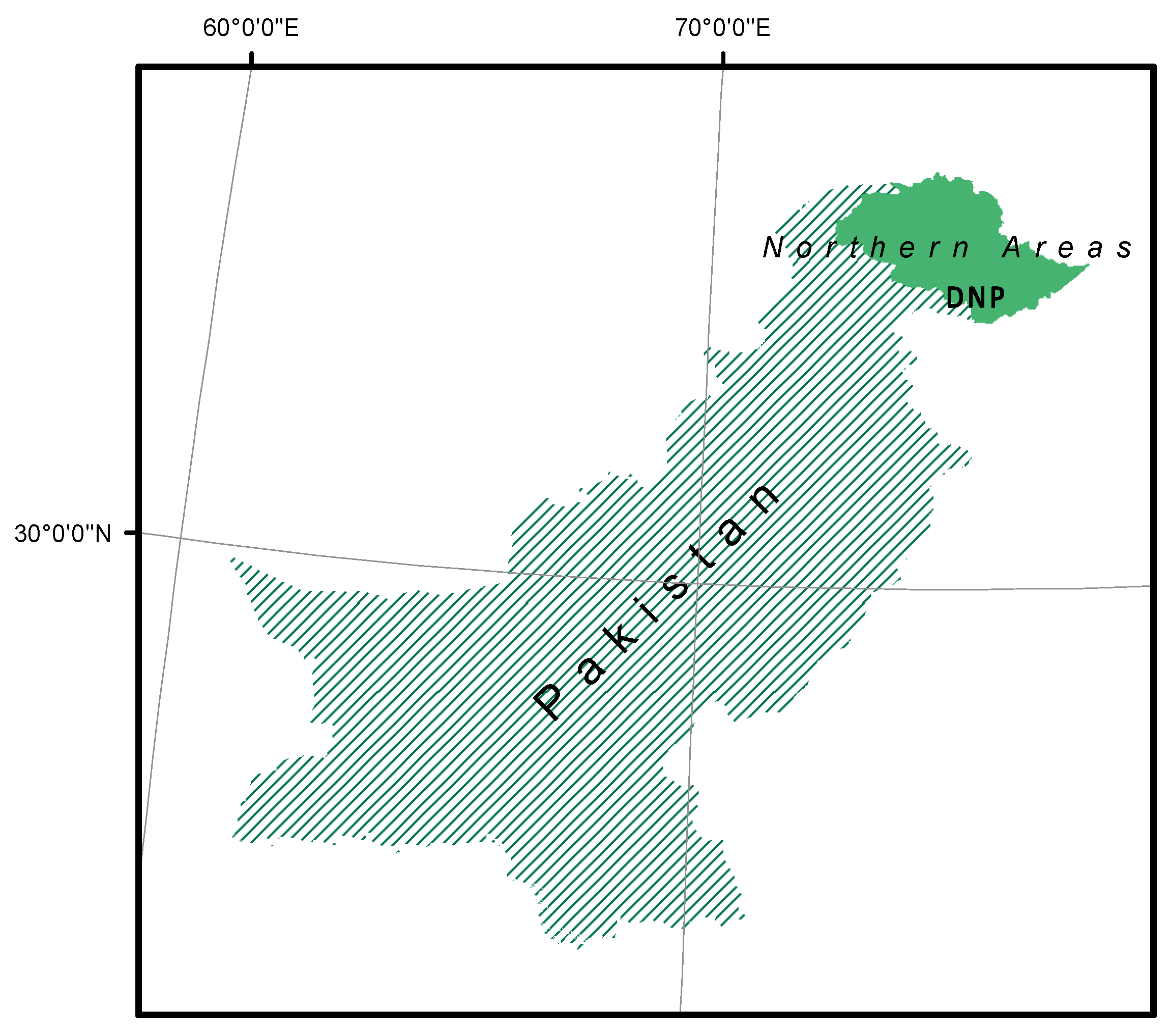
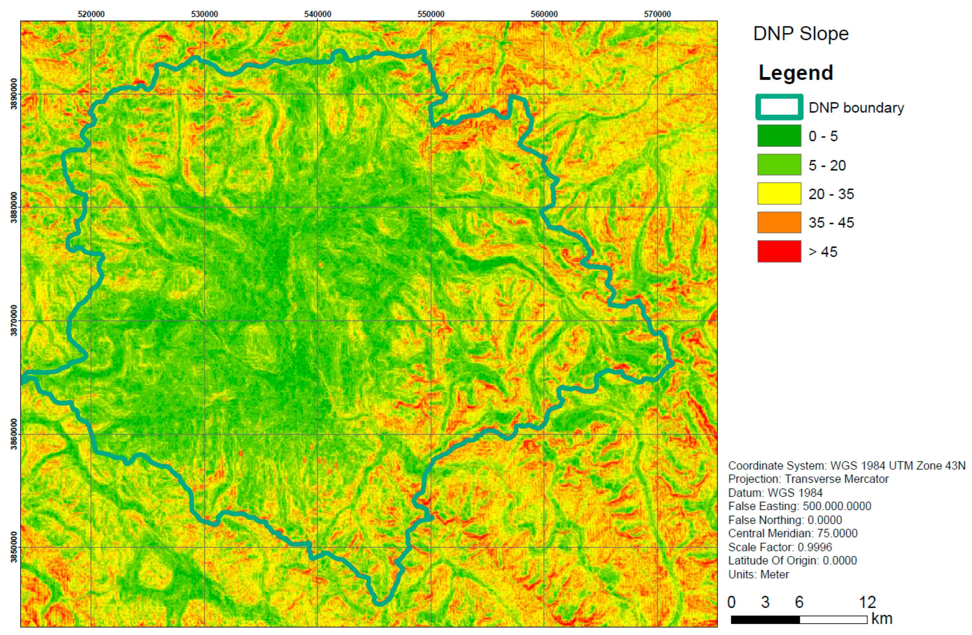
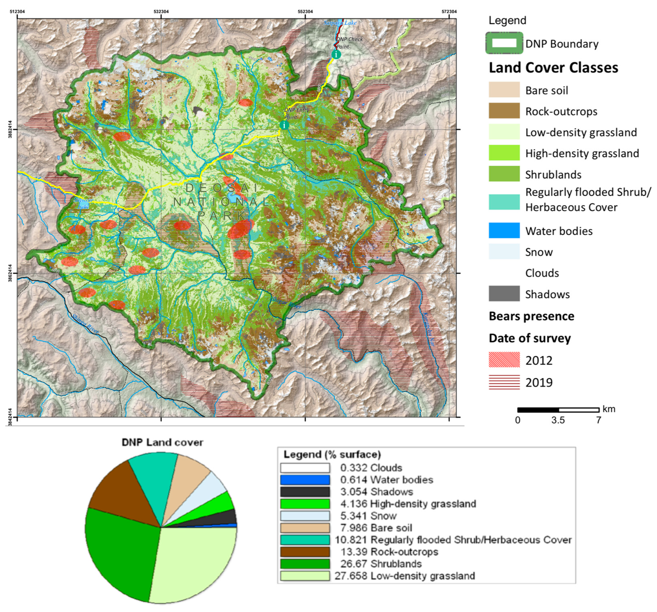
2. Study Area
3. Materials and Methods
3.1. Satellite Imagery
- Time-series of Landsat data
- ESA Sentinel 1
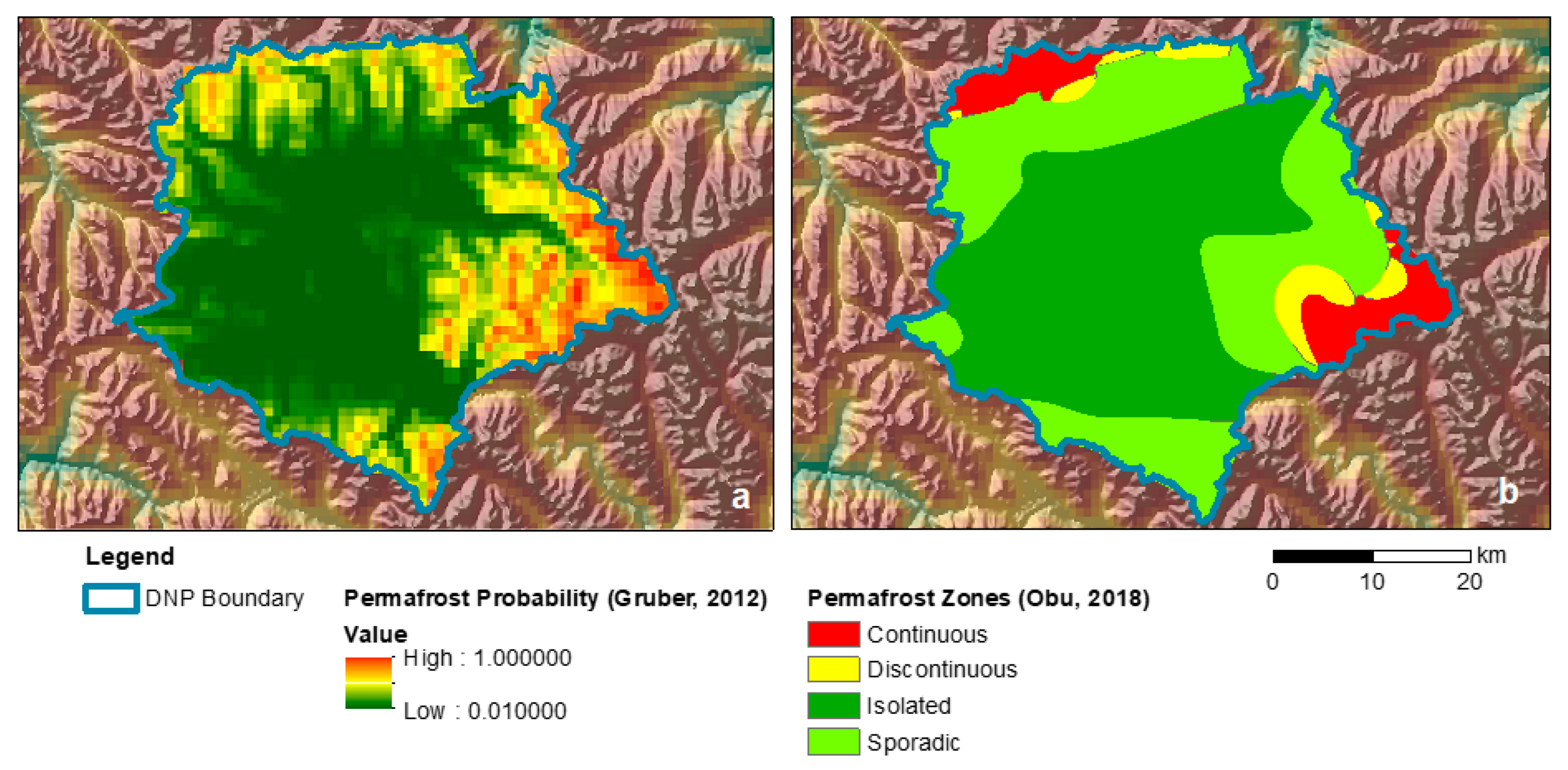
3.2. Permafrost Maps
- The Global Permafrost Zonation Index Map: The Global Permafrost Zonation Index Map has a resolution of 30 arc-seconds (about 1 km) and is available for all land areas except for Antarctica. It is available digitally for Google Earth, as a Web Mapping Service and, as raw data [9].
- The Permafrost Zonation: The product, at 1 km spatial resolution, provides the Permafrost probability (fraction values from 0 to 1). Each grid cell is classified as continuous, discontinuous and sporadic permafrost on the basis of its permafrost probability. It is provided also as classified shapefile [15].
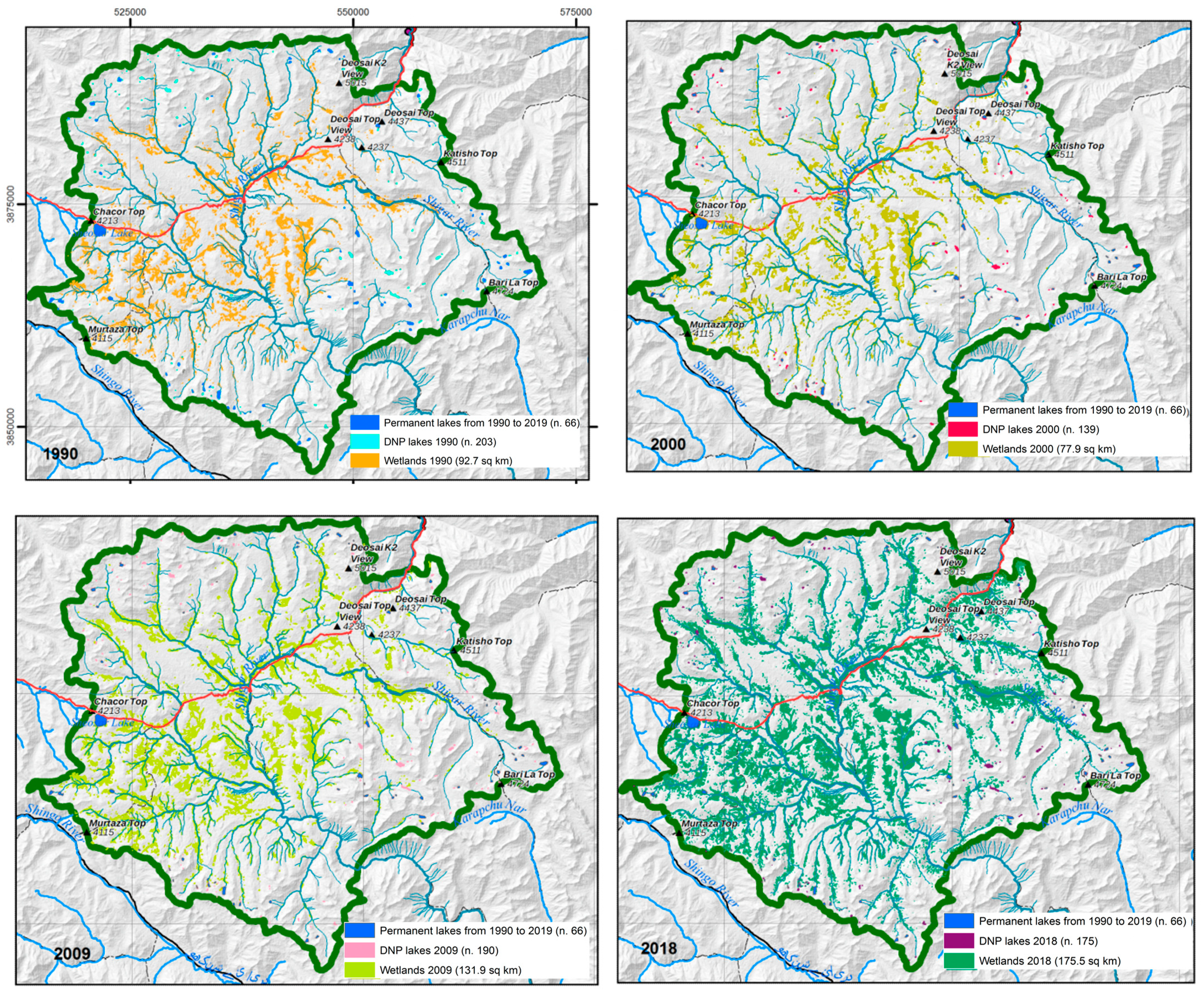
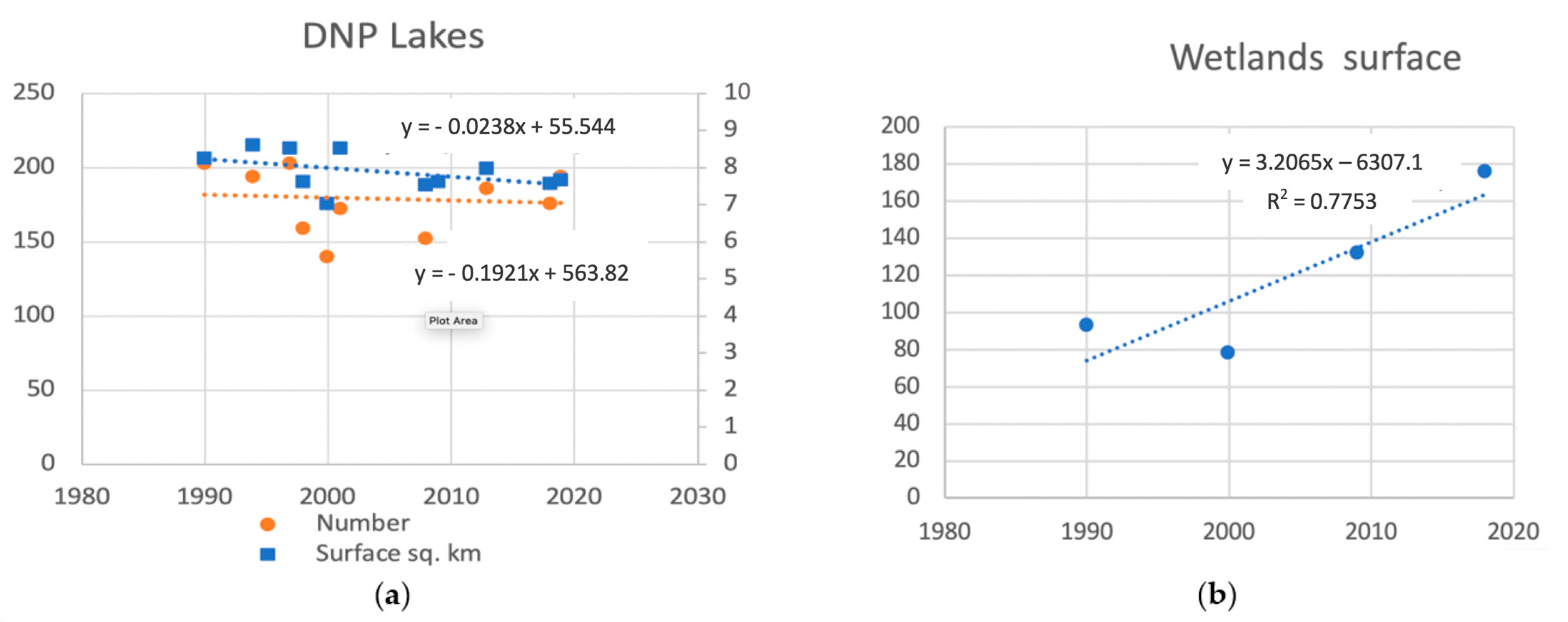
3.3. Lakes Extraction from Satellite Data
3.4. Wetlands Extraction
3.5. Terrain Displacement
4. Results
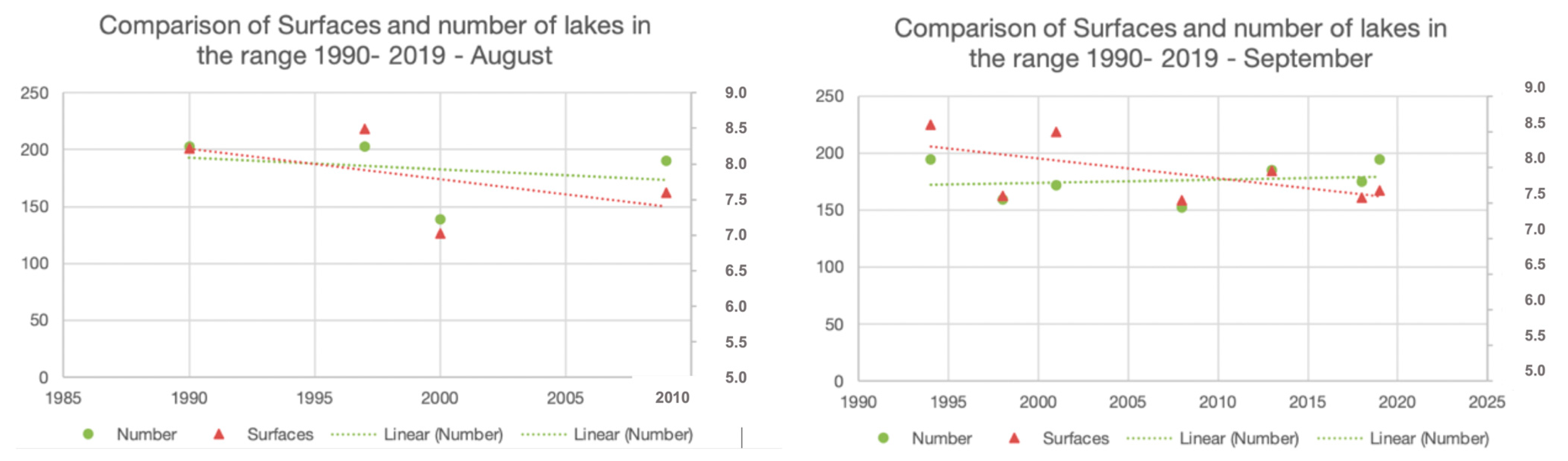
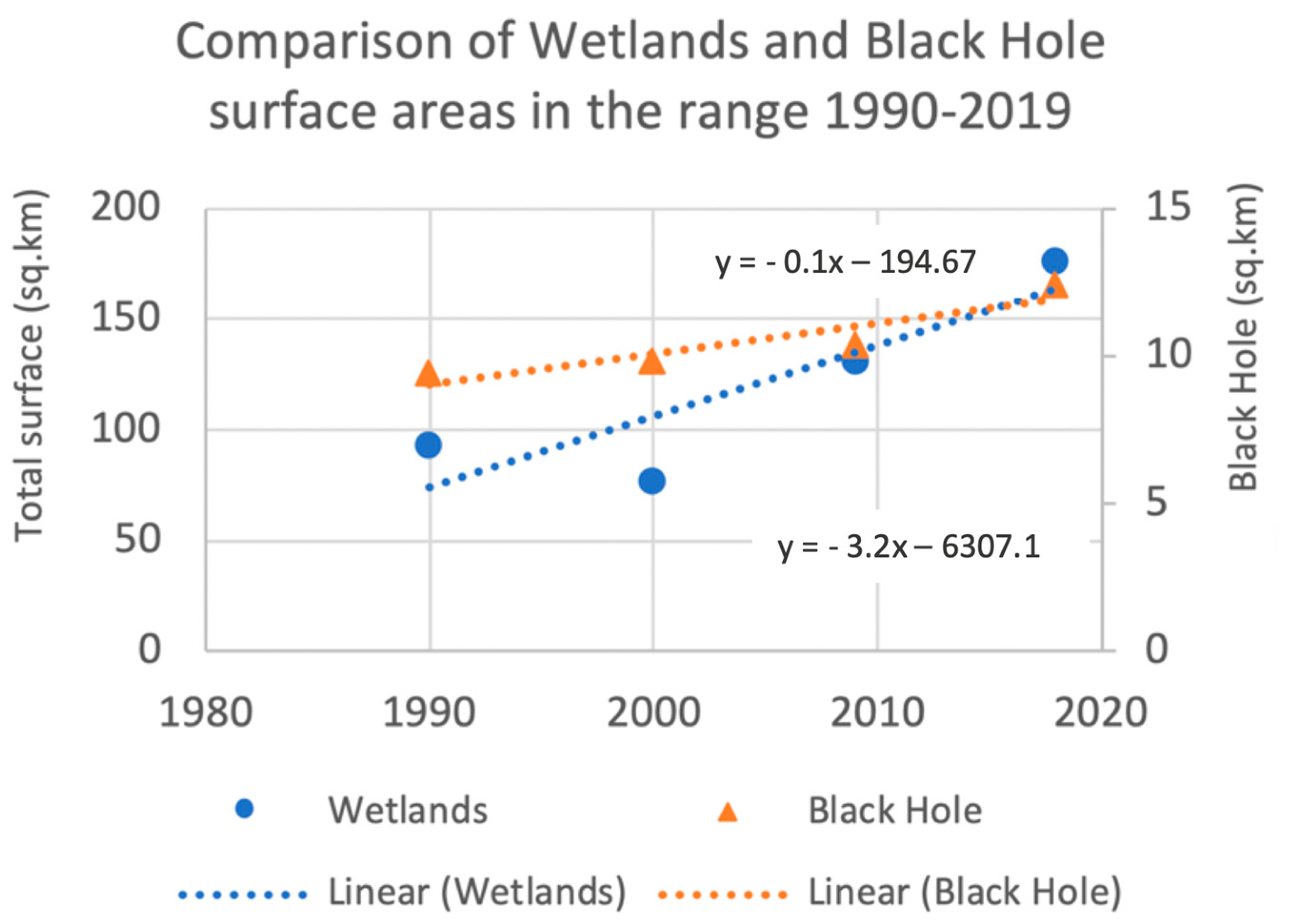
4.1. Optical Data
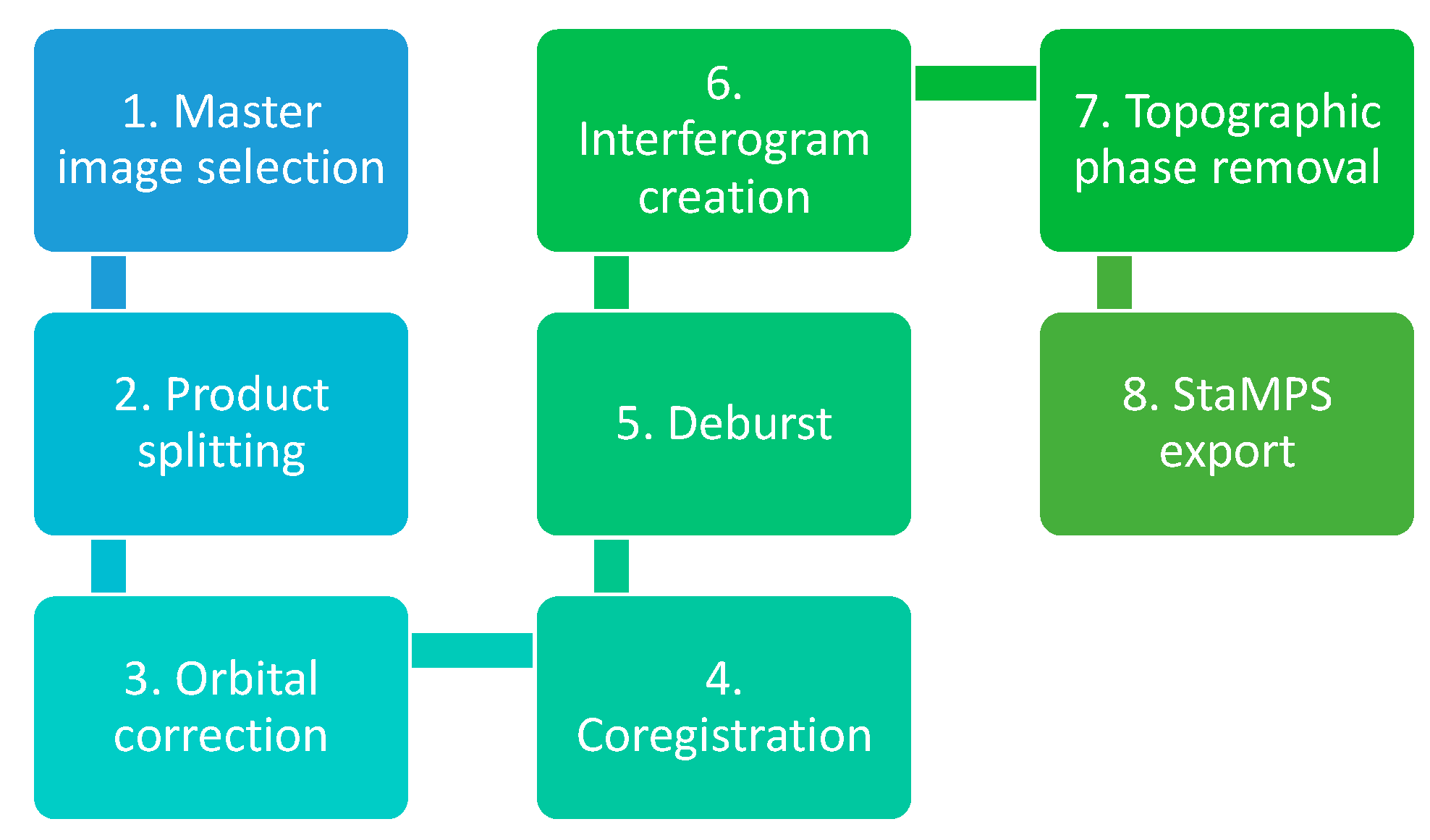
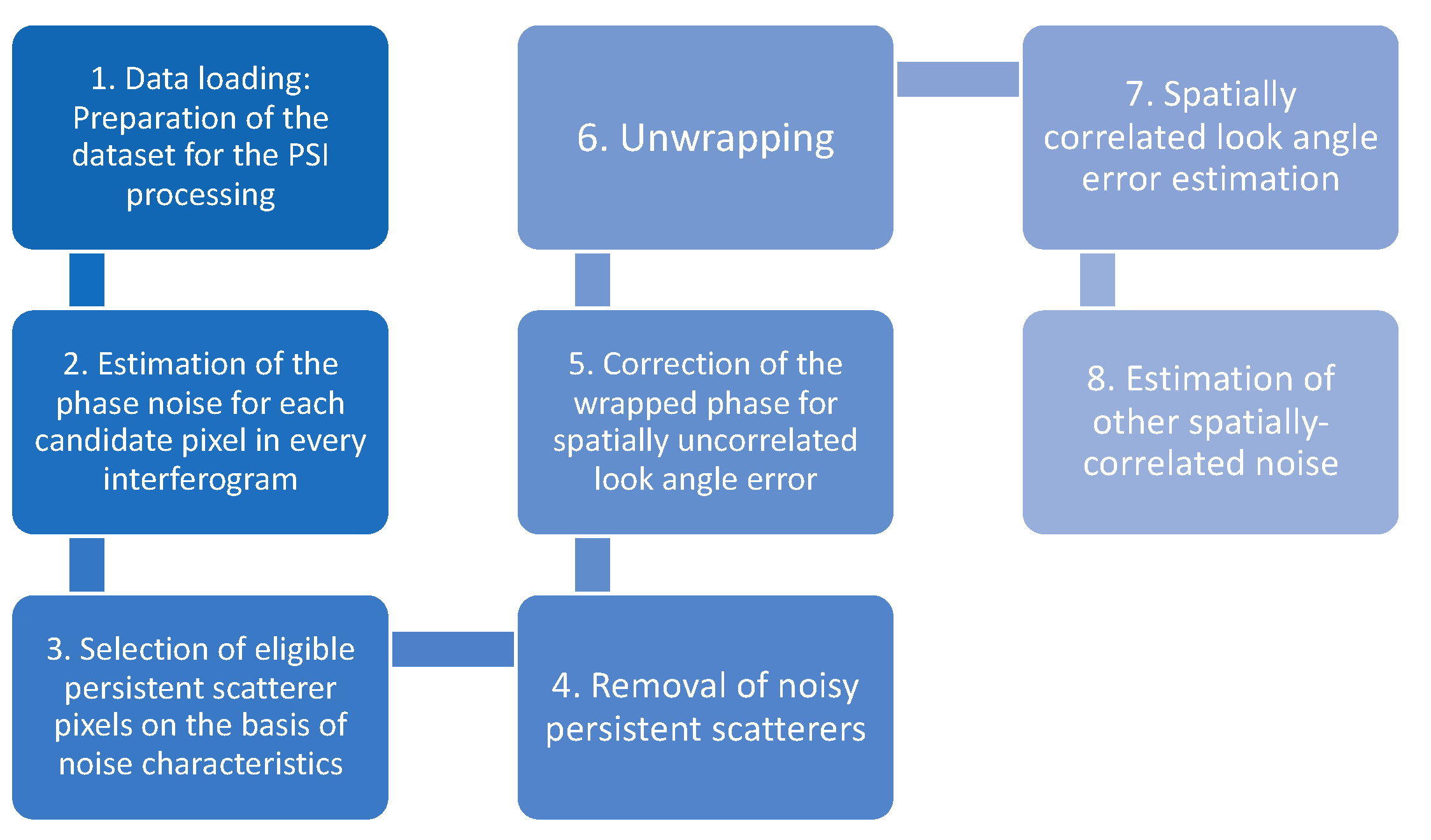
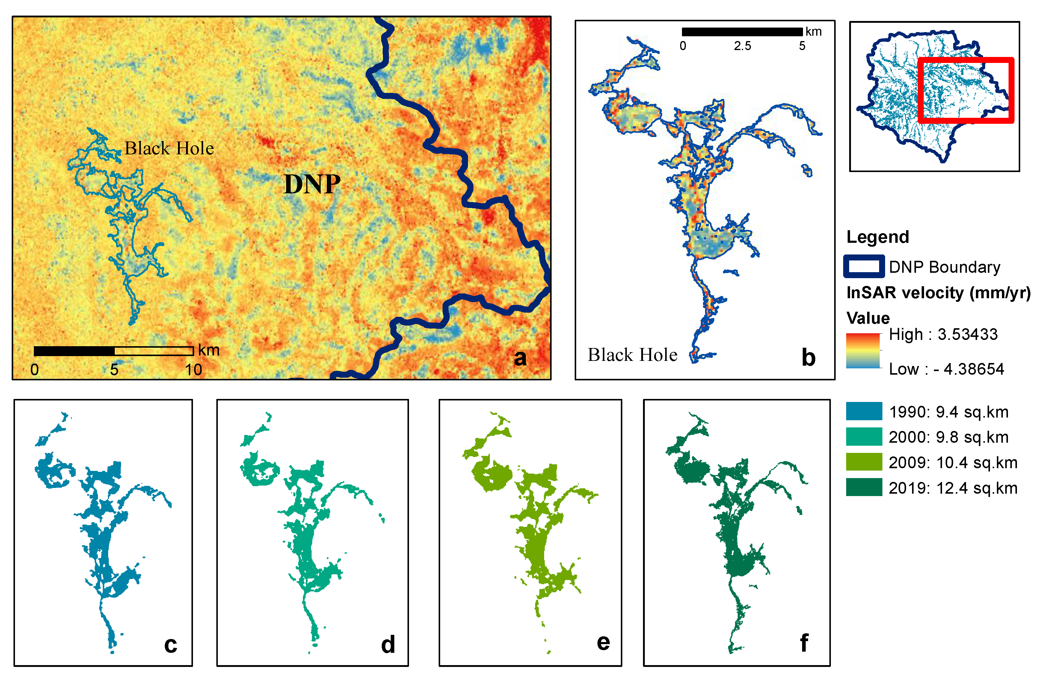
4.2. SAR Data
5. Discussion
6. Conclusions
Author Contributions
Funding
Acknowledgments
Conflicts of Interest
References
- Nawaz, M.A.; Swenson, J.E.; Zakaria, V. Pragmatic Management Increases a Flagship Species, the Himalayan Brown Bears, in Pakistan’s Deosai National Park. Biol. Conserv. 2008, 141, 2230–2241. [Google Scholar] [CrossRef]
- Nawaz, M.A.; Martin, J.; Swenson, J.E. Identifying Key Habitats to Conserve the Threatened Brown Bear in the Himalaya. Biol. Conserv. 2014, 170, 198–206. [Google Scholar] [CrossRef]
- Dar, S.A.; Singh, S.K.; Wan, H.Y.; Kumar, V.; Cushman, S.A.; Sathyakumar, S. Projected Climate Change Threatens Himalayan Brown Bear Habitat More than Human Land Use. Anim. Conserv. 2021, 24, 659–676. [Google Scholar] [CrossRef]
- Baig, S.U.; Malik, A.J.; Khan, H. Wildlife Habitat-Suitability Analysis for High Mountain National Parks in the Hindu Kush, Karakoram and Himalayan Region of Northern Pakistan. Model. Earth Syst. Environ. 2022, 8, 3941–3956. [Google Scholar] [CrossRef]
- Duan, P.; Wang, Y.; Yin, P. Remote Sensing Applications in Monitoring of Protected Areas: A Bibliometric Analysis. Remote Sens. 2020, 12, 772. [Google Scholar] [CrossRef] [Green Version]
- Melis, M.T.; Dessì, F.; Loddo, P.; Maccioni, A.; Gallo, M.; Ul Hassan, R.; Aurang Zaib, M. ESA Sentinel 2 Imagery and GBGEOApp: Integrated Tools for the Deosai National Park Management Plan. Int. Arch. Photogramm. Remote Sens. Spat. Inf. Sci. 2020, 43, 145–151. [Google Scholar] [CrossRef]
- Jadoon, U.K.; Ding, L.; Baral, U.; Qasim, M. Early Cretaceous to Eocene Magmatic Records in Ladakh Arc: Constraints from U–Pb Ages of Deosai Volcanics, Northern Pakistan. Geol. J. 2020, 55, 5384–5397. [Google Scholar] [CrossRef]
- Hussain, N.; Ali, S.; Hussain, A.; Ali, S.; Khan, S.W.; Raza, G.; Abbas, Q.; Hussain, I.; Hussain, M. Climate Change Variability Trends and Implications for Freshwater Resources in Pakistan’s Eastern Hindu Kush Region. Pol. J. Environ. Stud. 2018, 27, 665–673. [Google Scholar] [CrossRef]
- Gruber, S. Derivation and Analysis of a High-Resolution Estimate of Global Permafrost Zonation. Cryosphere 2012, 6, 221–233. [Google Scholar] [CrossRef] [Green Version]
- Zou, L.; Wang, C.; Tang, Y.; Zhang, B.; Zhang, H.; Dong, L. Interferometric SAR Observation of Permafrost Status in the Northern Qinghai-Tibet Plateau by ALOS, ALOS-2 and Sentinel-1 between 2007 and 2021. Remote Sens. 2022, 14, 1870. [Google Scholar] [CrossRef]
- Wang, S.; Xu, B.; Shan, W.; Shi, J.; Li, Z.; Feng, G. Monitoring the Degradation of Island Permafrost Using Time-Series InSAR Technique: A Case Study of Heihe, China. Sensors 2019, 19, 1364. [Google Scholar] [CrossRef] [Green Version]
- Chen, J.; Wu, T.; Zou, D.; Liu, L.; Wu, X.; Gong, W.; Zhu, X.; Li, R.; Hao, J.; Hu, G.; et al. Magnitudes and Patterns of Large-Scale Permafrost Ground Deformation Revealed by Sentinel-1 InSAR on the Central Qinghai-Tibet Plateau. Remote Sens. Environ. 2022, 268, 112778. [Google Scholar] [CrossRef]
- Short, N.; Brisco, B.; Couture, N.; Pollard, W.; Murnaghan, K.; Budkewitsch, P. A Comparison of TerraSAR-X, RADARSAT-2 and ALOS-PALSAR Interferometry for Monitoring Permafrost Environments, Case Study from Herschel Island, Canada. Remote Sens. Environ. 2011, 115, 3491–3506. [Google Scholar] [CrossRef]
- Rudy, A.C.A.; Lamoureux, S.F.; Treitz, P.; Short, N.; Brisco, B. Seasonal and Multi-Year Surface Displacements Measured by DInSAR in a High Arctic Permafrost Environment. Int. J. Appl. Earth Obs. Geoinf. 2018, 64, 51–61. [Google Scholar] [CrossRef]
- Obu, J.; Westermann, S.; Kääb, A.; Bartsch, A. Ground Temperature Map, 2000–2016, Northern Hemisphere Permafrost. Alfred Wegener Inst. Helmholtz Cent. Polar Mar. Res. Bremerhav. 2018. [Google Scholar] [CrossRef]
- Brown, J.; Romanovsky, V.E. Report from the International Permafrost Association: State of Permafrost in the First Decade of the 21st Century. Permafr. Periglac. Process. 2008, 19, 255–260. [Google Scholar] [CrossRef] [Green Version]
- Karlsson, J.M.; Lyon, S.W.; Destouni, G. Thermokarst Lake, Hydrological Flow and Water Balance Indicators of Permafrost Change in Western Siberia. J. Hydrol. 2012, 464–465, 459–466. [Google Scholar] [CrossRef]
- Yoshikawa, K.; Hinzman, L.D. Shrinking Thermokarst Ponds and Groundwater Dynamics in Discontinuous Permafrost near Council, Alaska. Permafr. Periglac. Process. 2003, 14, 151–160. [Google Scholar] [CrossRef]
- Meiners, S. The Glacial History of Landscape in the Batura Muztagh, NW Karakoram. GeoJournal 2005, 63, 49–90. [Google Scholar] [CrossRef]
- Iturrizaga, L. The Valley of Shimshal—A Geographical Portrait of a Remote High Mountain Settlement and Its Pastures with Reference to Environmental Habitat Conditions in the North-West Karakorum (Pakistan). GeoJournal 1997, 42, 303–328. [Google Scholar] [CrossRef]
- Gruber, S.; Fleiner, R.; Guegan, E.; Panday, P.; Schmid, M.-O.; Stumm, D.; Wester, P.; Zhang, Y.; Zhao, L. Review Article: Inferring Permafrost and Permafrost Thaw in the Mountains of the Hindu Kush Himalaya Region. Cryosphere 2017, 11, 81–99. [Google Scholar] [CrossRef] [Green Version]
- Freitas, P.; Vieira, G.; Canário, J.; Folhas, D.; Vincent, W.F. Identification of a Threshold Minimum Area for Reflectance Retrieval from Thermokarst Lakes and Ponds Using Full-Pixel Data from Sentinel-2. Remote Sens. 2019, 11, 657. [Google Scholar] [CrossRef] [Green Version]
- Villarroel, C.D.; Tamburini Beliveau, G.; Forte, A.P.; Monserrat, O.; Morvillo, M. DInSAR for a Regional Inventory of Active Rock Glaciers in the Dry Andes Mountains of Argentina and Chile with Sentinel-1 Data. Remote Sens. 2018, 10, 1588. [Google Scholar] [CrossRef] [Green Version]
- Rucci, A.; Ferretti, A.; Monti Guarnieri, A.; Rocca, F. Sentinel 1 SAR Interferometry Applications: The Outlook for Sub Millimeter Measurements. Sentin. Mission.-New Oppor. Sci. 2012, 120, 156–163. [Google Scholar] [CrossRef]
- Gabriel, A.K.; Goldstein, R.M.; Zebker, H.A. Mapping Small Elevation Changes over Large Areas: Differential Radar Interferometry. J. Geophys. Res. Solid Earth 1989, 94, 9183–9191. [Google Scholar] [CrossRef]
- Massonnet, D.; Feigl, K.L. Radar Interferometry and Its Application to Changes in the Earth’s Surface. Rev. Geophys. 1998, 36, 441–500. [Google Scholar] [CrossRef] [Green Version]
- Bürgmann, R.; Rosen, P.A.; Fielding, E.J. Synthetic Aperture Radar Interferometry to Measure Earth’s Surface Topography and Its Deformation. Annu. Rev. Earth Planet. Sci. 2000, 28, 169–209. [Google Scholar] [CrossRef]
- Ferretti, A.; Prati, C.; Rocca, F. Nonlinear Subsidence Rate Estimation Using Permanent Scatterers in Differential SAR Interferometry. IEEE Trans. Geosci. Remote Sens. 2000, 38, 2202–2212. [Google Scholar] [CrossRef] [Green Version]
- Ferretti, A.; Prati, C.; Rocca, F. Permanent Scatterers in SAR Interferometry. IEEE Trans. Geosci. Remote Sens. 2001, 39, 8–20. [Google Scholar] [CrossRef]
- Hooper, A.; Segall, P.; Zebker, H. Persistent Scatterer Interferometric Synthetic Aperture Radar for Crustal Deformation Analysis, with Application to Volcán Alcedo, Galápagos. J. Geophys. Res. Solid Earth 2007, 112, B07407. [Google Scholar] [CrossRef] [Green Version]
- Cian, F.; Blasco, J.M.D.; Carrera, L. Sentinel-1 for Monitoring Land Subsidence of Coastal Cities in Africa Using PSInSAR: A Methodology Based on the Integration of SNAP and StaMPS. Geosciences 2019, 9, 124. [Google Scholar] [CrossRef] [Green Version]
- Delgado Blasco, J.M.; Foumelis, M.; Stewart, C.; Hooper, A. Measuring Urban Subsidence in the Rome Metropolitan Area (Italy) with Sentinel-1 SNAP-StaMPS Persistent Scatterer Interferometry. Remote Sens. 2019, 11, 129. [Google Scholar] [CrossRef] [Green Version]
- Foumelis, M.; Delgado Blasco, J.M.; Desnos, Y.-L.; Engdahl, M.; Fernandez, D.; Veci, L.; Lu, J.; Wong, C. Esa Snap—Stamps Integrated Processing for Sentinel-1 Persistent Scatterer Interferometry. In Proceedings of the IGARSS 2018—2018 IEEE International Geoscience and Remote Sensing Symposium, Valencia, Spain, 22–27 July 2018; pp. 1364–1367. [Google Scholar]
- Mancini, F.; Grassi, F.; Cenni, N. A Workflow Based on SNAP–StaMPS Open-Source Tools and GNSS Data for PSI-Based Ground Deformation Using Dual-Orbit Sentinel-1 Data: Accuracy Assessment with Error Propagation Analysis. Remote Sens. 2021, 13, 753. [Google Scholar] [CrossRef]
- Bekaert, D.P.S.; Hooper, A.; Wright, T.J. A Spatially Variable Power Law Tropospheric Correction Technique for InSAR Data. J. Geophys. Res. Solid Earth 2015, 120, 1345–1356. [Google Scholar] [CrossRef]
- Foumelis, M. Vector-Based Approach for Combining Ascending and Descending Persistent Scatterers Interferometric Point Measurements. Geocarto Int. 2018, 33, 38–52. [Google Scholar] [CrossRef]
- Riordan, B.; Verbyla, D.; McGuire, A.D. Shrinking Ponds in Subarctic Alaska Based on 1950–2002 Remotely Sensed Images. J. Geophys. Res. Biogeosciences 2006, 111, G04002. [Google Scholar] [CrossRef]
- Smith, L.C.; Sheng, Y.; MacDonald, G.M.; Hinzman, L.D. Disappearing Arctic Lakes. Science 2005, 308, 1429. [Google Scholar] [CrossRef] [Green Version]
- Sannel, A.B.K.; Kuhry, P. Warming-Induced Destabilization of Peat Plateau/Thermokarst Lake Complexes. J. Geophys. Res. Biogeosciences 2011, 116, G030035. [Google Scholar] [CrossRef]
- Hassan, J.; Chen, X.; Muhammad, S.; Bazai, N.A. Rock Glacier Inventory, Permafrost Probability Distribution Modeling and Associated Hazards in the Hunza River Basin, Western Karakoram, Pakistan. Sci. Total Environ. 2021, 782, 146833. [Google Scholar] [CrossRef] [PubMed]
- Schmid, M.-O.; Baral, P.; Gruber, S.; Shahi, S.; Shrestha, T.; Stumm, D.; Wester, P. Assessment of Permafrost Distribution Maps in the Hindu Kush Himalayan Region Using Rock Glaciers Mapped in Google Earth. Cryosphere 2015, 9, 2089–2099. [Google Scholar] [CrossRef] [Green Version]
- Colombo, N.; Salerno, F.; Martin, M.; Malandrino, M.; Giardino, M.; Serra, E.; Godone, D.; Said-Pullicino, D.; Fratianni, S.; Paro, L.; et al. Influence of Permafrost, Rock and Ice Glaciers on Chemistry of High-Elevation Ponds (NW Italian Alps). Sci. Total Environ. 2019, 685, 886–901. [Google Scholar] [CrossRef] [PubMed]
- Melis, M.T.; Pisani, L.; De Waele, J. On the Use of Tri-Stereo Pleiades Images for the Morphometric Measurement of Dolines in the Basaltic Plateau of Azrou (Middle Atlas, Morocco). Remote Sens. 2021, 13, 4087. [Google Scholar] [CrossRef]


| Satellite | Path | Acquisition Date |
|---|---|---|
| Landsat 4-5 | 149-36 | 7 August 1990 |
| Landsat 4-5 | 149-36 | 3 September 1994 |
| Landsat 4-5 | 149-36 | 10 August 1997 |
| Landsat 4-5 | 149-36 | 30 September 1998 |
| Landsat 4-5 | 149-36 | 16 August 1999 |
| Landsat 7 | 149-36 | 26 August 2000 |
| Landsat 7 | 149-36 | 30 September 2001 |
| Landsat 4-5 | 149-36 | 25 September 2008 |
| Landsat 4-5 | 149-36 | 27 August 2009 |
| Landsat 8 | 149-36 | 7 September 2013 |
| Landsat 8 | 149-36 | 17 August 2017 |
| Landsat 8 | 149-36 | 21 September 2018 |
| Landsat 8 | 149-36 | 24 September 2019 |
| Orbit | Number of Images | Master Image Date | Time Reference | |
|---|---|---|---|---|
| Start | End | |||
| Ascending | 26 | 18 August 2019 | 15 July 2014 | 31 August 2022 |
| Descending | 16 | 29 August 2017 | ||
| Acquisition Year | Acquisition Month | Total Surface (sq. km) | Total Number of Lakes |
|---|---|---|---|
| 1990 | August | 11.4 | 203 |
| 1994 | September | 11.1 | 220 |
| 1997 | August | 11.3 | 240 |
| 1998 | September | 10.7 | 186 |
| 1999 | August | 8.2 | 164 |
| 2000 | August | 10.1 | 221 |
| 2001 | September | 11.4 | 227 |
| 2008 | September | 10.3 | 198 |
| 2009 | August | 10.6 | 253 |
| 2013 | September | 10.9 | 256 |
| 2017 | August | 8.7 | 216 |
| 2018 | September | 10.1 | 232 |
| 2019 | September | 9.9 | 217 |
| Date of Acquisition | Wetlands Surface (sq. km) |
|---|---|
| 1990 | 92.7 |
| 2000 | 77.9 |
| 2009 | 13.9 |
| 2018 | 175.5 |
| Max Value (mm/yr) | Min Value (mm/yr) | Standard Dev. | Median | Q1 | Q3 | IQR |
|---|---|---|---|---|---|---|
| 5.207 ± 0.1 | −6.235 ± 0.1 | 0.749 | 0.129 | −0.317 | 0.524 | 0.841 |
Disclaimer/Publisher’s Note: The statements, opinions and data contained in all publications are solely those of the individual author(s) and contributor(s) and not of MDPI and/or the editor(s). MDPI and/or the editor(s) disclaim responsibility for any injury to people or property resulting from any ideas, methods, instructions or products referred to in the content. |
© 2023 by the authors. Licensee MDPI, Basel, Switzerland. This article is an open access article distributed under the terms and conditions of the Creative Commons Attribution (CC BY) license (https://creativecommons.org/licenses/by/4.0/).
Share and Cite
Melis, M.T.; Dessì, F.G.; Casu, M. New Remote Sensing Data on the Potential Presence of Permafrost in the Deosai Plateau in the Himalayan Portion of Pakistan. Remote Sens. 2023, 15, 1800. https://doi.org/10.3390/rs15071800
Melis MT, Dessì FG, Casu M. New Remote Sensing Data on the Potential Presence of Permafrost in the Deosai Plateau in the Himalayan Portion of Pakistan. Remote Sensing. 2023; 15(7):1800. https://doi.org/10.3390/rs15071800
Chicago/Turabian StyleMelis, Maria Teresa, Francesco Gabriele Dessì, and Marco Casu. 2023. "New Remote Sensing Data on the Potential Presence of Permafrost in the Deosai Plateau in the Himalayan Portion of Pakistan" Remote Sensing 15, no. 7: 1800. https://doi.org/10.3390/rs15071800