1. Introduction
Soil moisture (SM) and land surface temperature (LST) are land surface state variables that control surface energy and water fluxes, land–atmosphere interactions and terrestrial processes. They are indispensable to climate, ecology, agriculture, and other fields [
1,
2,
3]. The timely and effective acquisition of SM and LST is of great practical significance for regional climate and agricultural monitoring, and it has broad application prospects. Remote sensing technology has the ability to accurately monitor many elements in the earth system at the global scale and allows us to quickly and effectively obtain SM and LST over large-scale domains. In particular, passive microwave remote sensing has all-weather monitoring capabilities and strong penetration abilities with respect to clouds and rain. It is also very sensitive to changes in SM, and LST, and has been widely used in the monitoring and retrieval of surface parameters [
4,
5,
6]. The emissivity at the microwave bands is mainly controlled by the dielectric constant, which itself is a function of SM, roughness, LST, soil salinity, and vegetation type and structure [
7]. Among all influencing factors, SM changes have the largest impact on the dielectric constant and the influence of other factors is relatively stable for bare areas [
4]. Therefore, land surface emissivity (LSE) is mainly controlled by SM and thus has the signature of retrieving SM. The brightness temperature (
T𝐵) is recorded by satellite. LST should be known a priori to estimate the LSE from
T𝐵 via
T𝐵 = LST × LSE. On the other hand, to retrieve LST from
T𝐵 measurements, LSE should be known, which itself is mainly controlled by the SM [
4]. Therefore, SM and LST are entangled and the estimation of each of them requires a priori knowledge of the other one. This raises the question of how to retrieve two interrelated variables. Although there have been many studies on passive microwave retrieval of SM [
8,
9,
10,
11], there is not a solid approach for obtaining high-precision LST [
5,
12,
13].
The existing SM retrieval methods fall into five main groupings [
14]: (1) the operational algorithm adopted by NASA, which is referred to as the Normalized Polarization Difference (NPD) algorithm [
15], (2) the Single Channel Algorithm (SCA) [
16,
17], (3) the Land Parameter Retrieval Model (LPRM) [
18,
19], (4) the University of Montana (UMT) soil moisture algorithm [
20], and (5) the HydroAlgo Artificial Neural Network (HA-ANN) algorithm [
9,
21,
22]. The majority of these approaches work based on the Radiative Transfer Equation (RTE), but the treatment of the key parameter of surface temperature in the soil moisture retrieval process is different. The SM retrieval equations are simplified to be independent of LST for the operational NPD algorithm. The SCA and LPRM estimates LST from brightness temperature via a regression-based equation. UMT obtains LST by a geophysical radiative transfer model. The HA-ANN algorithm does not use LST as an input parameter. Many studies have used neural networks to retrieve geophysical parameters [
23,
24,
25,
26,
27,
28,
29,
30], but the computational process of the hidden layers of neural networks needs further interpretation and research.
Passive microwave remote sensing can rapidly achieve global coverage and help us study the spatiotemporal changes of LST in large-scale regions [
12,
31]. However, due to the variation of surface emissivity with SM, it is difficult to accurately retrieve LST from passive microwave remote sensing data. There are two main methods for retrieving LST from passive microwave remote sensing data. The first is the statistical method, which includes single-channel statistical methods [
32] and multi-channel statistical methods [
4,
33]. The other method is the neural network algorithm, which also directly uses the brightness temperature to retrieve LST without considering the changes of SM [
34,
35].
For passive microwave remote sensing, most existing algorithms do not consider the mutual influence of SM and LST changes over time; the main reason is that it is very difficult to capture their respective dynamic changes. Some physical retrieval methods of geophysical variables have to utilize empirical equations, which cannot accurately represent the problem, thus making the overall retrieval weak [
36]. Statistical methods are mainly applicable to local areas [
30]. Although there are also studies using neural networks or deep learning to retrieve soil moisture or surface temperature from passive microwave data [
9,
23,
24,
37,
38], some of them are not very portable. The main reason is that training and testing data mainly come from statistical sampling, which limits both the retrieval accuracy and the range of applications. However, most of these studies have not clearly explained why and how to use deep learning to obtain better results from physical mechanisms. They also have not used the mutual prior knowledge of SM and LST to perform cross iteration to improve retrieval accuracy. In this study, we propose a “Geophysical Parameter Retrieval Paradigm Theory”, which uses deep learning technology to integrate physical methods, statistical methods, and expert knowledge to improve the retrieval accuracy of LST and SM from passive microwave remote sensing data. The fully coupled SM-LST algorithm can overcome the shortcomings of previous algorithms and make full use of the respective advantages of physical methods and deep learning methods. This paradigm retrieval theory maintains the physical meaning of the method, and deep learning is only used for optimization calculations, which makes the application of deep learning physically interpretable.
2. Methodology
The retrieval paradigm of geophysical parameters proposed by us is that a complete set of closed-form equations can be constructed between the input parameters and output parameters of deep learning in theory. If there is a strong correlation between input parameters and output parameters, deep learning can be directly used for inversion. If there is a weak correlation between input parameters and output parameters, it is necessary to add prior knowledge to improve the inversion accuracy of output parameters. If we know a large number of representative solutions of the physical method, we can use deep learning to obtain the curve function of the solution through training. Physical model simulations provide us with the opportunity to obtain solutions of physical methods, so deep learning can replicate physical methods. Physical methods cannot describe all situations, and we can supplement solutions of statistics methods with multi-source data.
The main hypothesis behind “Geophysical Parameter Retrieval Paradigm Theory” is that if the target information (problem) can be described by a mathematical equation (which form the only solution curve in the space), then deep learning can couple the physical and traditional statistical methods through big data learning and optimization. The proposed paradigm not only maintains the physical significance of the method and the advantages of the statistical method, but also utilizes the optimization ability of deep learning to maximizes the retrieval accuracy of SM and LST. Here we give a classic case of remote sensing retrieval of geophysical parameters. Based on the entangled relationship between SM and LST, a model-data-knowledge driven collaborative retrieval (MDK-CR) method for SM and LST is proposed. The flow chart of the MDK-CR method based on artificial intelligence is shown as in
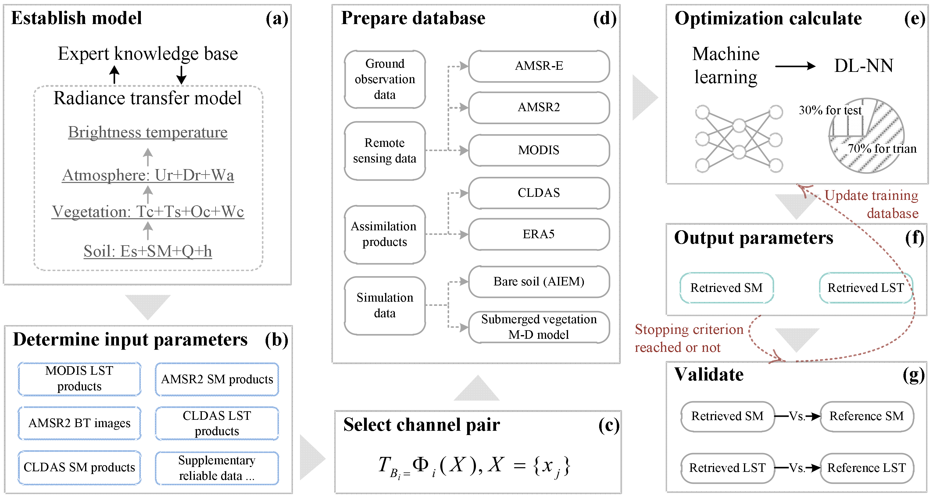
Figure 1, which can unify various methods through smartly utilizing deep learning for interleaved iterative optimization computations. The proposed approach can be summarized via the following steps:
Step (a): According to the specific passive microwave data, the physical mechanism of SM and LST retrieval is derived based on expert knowledge, and then logical rules are established to determine the mutual prior knowledge of SM and LST (
Section 3.2). Finally, the best retrieval scheme is constructed for the specific data (
Section 3.3).
Step (b): The details are in
Section 3.1. The simulation data obtained from the physical model, image brightness temperature data with corresponding high precision SM and LST product data, assimilation product data, and ground observation site data, are used as the training and testing sample of the deep learning neural network (DL-NN). The sample space can represent physical algorithms and statistical methods, and we use big data and deep learning to integrate physical and statistical methods.
Step (c): Build a DL-NN for SM and LST collaborative retrieval. To overcome the shortcomings of previous machine learning iterations on only one parameter (SM or LST) and the entanglement of surface temperature and soil moisture, we smartly design interleaved iterative optimization computations for SM and LST.
Step (d): For SM, the brightness temperatures of low frequency bands of passive microwaves are used as the input value of DL-NN input nodes while the corresponding SM is used as the output value, and the optimal number of hidden layers and hidden nodes are found for SM retrieval.
Step (e): The SM obtained in step (d) or step (f) and the brightness temperature of passive microwave high frequency bands are used as the input values of the neural network input node while the corresponding LST is used as the output value. Similarly, the best number of hidden layers and hidden nodes is found for LST retrieval.
Step (f): The LST obtained in step (e) and the brightness temperatures of passive microwave low frequency bands are used as the input values of the neural network input node, and the corresponding SM is used as the output value. Similarly, the best number of hidden layers and hidden nodes is again found for SM retrieval, and then one can repeat step (e) until the accuracy of the soil moisture and surface temperature retrieval no longer improves and then stop the iteration.
Step (g): The accuracy of the trained DL-NN is verified by the testing data, and the retrieval results are obtained. The specific and detailed implementation process of the abovementioned algorithm refers to
Section 3 and
Section 4.
Figure 1.
The proposed MDK-CR method consists of two parts: geophysical logical reasoning based on the RTE (Steps (a–d)), and an iterative optimization algorithm using a deep learning neural network (DL-NN) (Steps (e–g)). In Step (a), The brightness temperature at satellite includes contributions from the soil (emissivity (Es), soil moisture (SM), roughness parameters (Q & h)), vegetation (vegetation canopy temperature (Tc), soil temperatures (Ts), vegetation opacity (Oc) and vegetation water content (Wc)), and atmosphere (upwelling atmospheric radiance (Ur), downwelling atmospheric radiance (Dr), atmosphere water vapor (Wa)). Models and characteristics of land surface microwave emission have been studied extensively; and are roughness parameters. In Step (c), the model function relates the parameters of the soil-vegetation-atmosphere medium to the brightness temperature observations at channel .
3. Materials and Methods
3.1. Data
Multi-source data including physical model simulations, ground observations, remote sensing data, and assimilation products (the fifth generation of ECMWF reanalysis (ERA5), and China Land Data Assimilation System (CLDAS)) were used to generate the training and test datasets. Each of these data streams is explained below.
(1) Remote sensing data.
We used the brightness temperatures of AMSR2 as known independent variables in our SM and LST retrieval algorithm. AMSR2 is a second-generation advanced microwave radiation imager, which is installed on the “Global Change Observation Mission—Water (GCOM-W1)” by the Japan Aerospace Exploration Agency (JAXA) and successfully launched in 2012. The AMSR2 daily brightness temperature level three product is available to the public from JAXA (gportal.jaxa.jp). At present, AMSR2 SM products mainly have two sets of data: the official soil moisture product of JAXA produced by a lookup table algorithm and the soil moisture product of the University of Amsterdam in the Netherlands produced by the land surface parameter retrieval model LPRM (Land Surface Parameter Model) algorithm. We used 10 km of JAXA L3 grade AMSR2 SM products and corresponding brightness temperature data at satellite, which has been widely recognized [
39,
40,
41].
The MODIS surface temperature product is used as the source of the corresponding surface temperature data. MODIS is mounted on Terra and Aqua satellites [
42]. Terra’s orbit around the Earth is timed so that it passes descending from north to south across the equator in the morning (10:30 a.m.), while Aqua passes south to north over the equator ascending in the afternoon (1:30 p.m.). The data are updated at least twice a day, and MODIS LST products (MYD11C1) have been widely applied in many fields [
2,
6,
42,
43,
44]. MYD11C1 data with a time resolution of one day and a spatial resolution of 10 km are used in this study, and the accuracy of the LST product is generally recognized and has been well verified [
42,
44].
(2) Simulation data of AIEM and M-D.
Under the conditions of setting 0.5 < sig < 3.5, 3 < cl < 35, 0.02 < SM < 0.45, 270 K < LST < 325 K, the SM and LST simulation data are generated using the advanced integral equation model (AIEM) [
45] and the matrix doubling (M-D) model [
46]. AIEM was developed based on the Integral Equation Model (IEM). The M-D model presents relatively high accuracy in simulating SM because the algorithm fully considers multiple scattering within vegetation and between vegetation and the surface [
46]. In this study, we use two models to simulate TB with the corresponding SM and LST which is used for the training and test data in a DL-NN.
(3) SM and LST assimilation products.
ERA5 is the fifth-generation ECMWF (the European Centre for Medium-Range Weather Forecasts) atmospheric reanalysis global climate data, which covers the period from January 1950 onwards, and provides hourly estimates of atmospheric, land, and ocean climate variables. The resolution of most of the variables is 30 km, and the resolution of some land parameters is 0.1°. In recent years, this data set has been widely used and the accuracy of the parameters has been improved compared to the previous version [
47,
48,
49]. We used ERA5 LST data (0.1°) and SM data (0.1°) at a depth of 0–7 cm underground.
The CLDAS (China Land Data Assimilation System) data product from the China Meteorological Administration covers the Asian region (0–65°N, 60–160°E) [
50]. CLDAS uses data fusion and assimilation technology to integrate multisource data (e.g., ground observation data, satellite remote sensing data, and numerical model products) to generate meteorological variables such as air and surface temperature, soil moisture, air pressure, humidity, wind speed, precipitation, and radiation. The SM and LST data are from the CLDAS-V1.0 business system, which are released to the public by the China Meteorological Data Network. The CLDAS dataset includes hourly soil moisture and soil temperature data with a spatial resolution of 0.0625° × 0.0625° at depths of 0–5, 0–10, 10–40, 40–100, and 100–200 cm in East Asia. Surface temperature and soil moisture at the depth of 0–5 cm were used in this study. The CLDAS SM and LST data were resampled to a resolution of 10 km to be consistent with those of AMSR2. When collecting data, only ground observation data close to ERA5 and CLDAS data values will be used, and abnormal and unrepresentative data should be eliminated to ensure that the selected data reflect all physical conditions.
3.2. Geophysical Logical Reasoning Driven by Expert Knowledge
The SM-LST retrieval algorithm is based on the radiative transfer (RT) process that relates surface and atmospheric variables to the brightness temperature observations. In the proposed SM-LST retrieval paradigm, the deep learning network finds the relationship between inputs (brightness temperatures) and outputs (SM and LST).
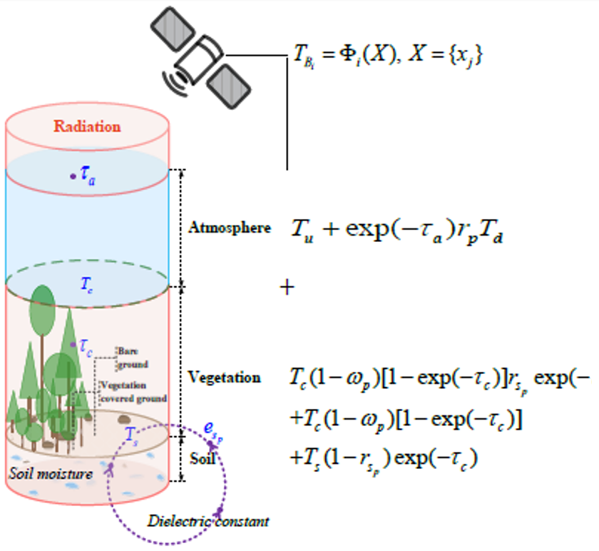
Figure 2 shows the physical derivation of SM and LST based on the RT modeling.
The SM and LST retrieval are based on modeling the thermal radiance from the bare soil, vegetated soil, and canopy. For bare soil, LSE mainly changes with SM and ground roughness. Atmospheric water vapor influences satellite radiance measurements at several frequencies. The space-borne brightness temperature (
TBi) measurements in channel
i can be related to the state variables of land surface (i.e., SM and LST) via the model function Φ
i(
X), as in Equation (1):
In this study, in order to improve the retrieval accuracy of LST and SM, we considered the influence of atmospheric water vapor on brightness temperature at satellite, and the soil and vegetation temperatures were retrieved as a single effective surface temperature averaged over the satellite footprint. Three surface radiation models were used depending on the surface roughness.
(1) Smooth surfaces radiometric modelling.
For a smooth surface, the brightness temperature (
TBp), (where p represents polarization, H or V) is related to the effective land surface temperature (
Ts) and via:
where
Ts is the effective land surface temperature,
θ is the incidence (observation) angle relative to nadir, and
esp is the LSE that can be computed from the land surface reflectivity Γ
bp [
51]:
Using the Fresnel equations for smooth surfaces, soil reflectivity (Γ
Bp*) can be computed from the soil dielectric constant (
ε) and incidence angle (
θ) (Equations (4) and (5)). The dielectric constant at a given frequency depends on SM and, to a lesser extent, on the soil density and percentage of sand and clay. The Dobson dielectric model is used in this study to estimate the soil dielectric constant [
52].
According to the Fresnel formulas (Equations (4) and (5)), the reflectivity of a smooth surface under H and V polarizations is related to the soil dielectric constant,
ε (which itself depends on SM) and observation angle (
θ). Given the brightness temperature measurements (
TBp) in Equation (1), Ts,
θ, and
esp (which itself is a function of SM) are the three unknowns.
(2) Rough surface radiometric modelling.
A smooth land surface is a special case of a rough surface. Hence, the influence of roughness should be considered in surface radiation modeling. Moreover, since microwave radiation penetrates into the ground, the volume scattering (caused by uneven physical properties of the soil) must be considered. Semi-empirical and physical models have been used to calculate the emissivity of rough surfaces [
52].
In this study, the semi-empirical L-MEB model, which was developed by Wang and Choudhury [
53], was used to analyze the roughness surface. The rough surface reflectivity (Γ
𝐵𝑝) can be written as follows:
where
and
(with 𝑝1 = H and 𝑝2 = V) are the specular reflectivity of a smooth surface for the horizontal and vertical polarizations, respectively. H
RP, Q
R and N
PR are the roughness parameters, as in Equation (7):
where
HQN is roughness model,
s and
l are the root mean square height and correlation length, respectively, which are used to describe surface roughness. Therefore, given the brightness temperature measurements (
TBp) in Equation (1), there are five main unknowns in the case of a rough surface— SM, LST,
θ,
s, and
l, so at least five equations must be constructed to solve the SM and LST.
(3) Vegetation radiometric modeling.
For a vegetated land surface, the soil, vegetation, and atmosphere contribute to the brightness temperature measurements of the satellite. The contribution of the atmosphere (
TA) to the brightness temperature is given by Equation (8).
where
Tu and
Td are the upwelling and downwelling atmospheric emissions, respectively.
τa is the atmospheric opacity along the viewing path, which depends on water vapor content (WVC).
rp is the surface reflectivity. The brightness temperature (
Tbp) for a homogeneous vegetated surface can be calculated by Equation (9). After considering the influence of the atmosphere, the whole radiative transfer (RT) process can be described by Equation (10).
Here, the LSE (
esp) and reflectivity (
rsp) are related by
esp = 1 −
rsp,
τc which is the vegetation opacity along the viewing path while
ωp is the vegetation single scattering albedo. Multiple scattering in the vegetation layer is neglected, and the soil and vegetation temperatures
Ts are assumed to be approximately equal [
4]. The opacity along the viewing path is related to the vegetation water content by Equation (11):
where b is the statistical coefficient and
ωe is the vegetation water content. Therefore, for vegetated land surface, there are nine unknowns, namely, SM, LST,
esp,
ωp,
ωe, s, l, θ, and WVC. Bare surface is considered a special case of a vegetated surface.
Given the abovementioned nine unknown variables, nine equations are required for the simultaneous retrieval of SM and LST on a vegetated surface. Since there is an inherent connection (e.g., Equation (6)) among the different physical parameters, we compared the retrieval accuracy at different frequencies by constructing different combinations with eight to fourteen radiative transfer equations. Low frequencies are more sensitive to SM. Hence, brightness temperatures in at least eight low-frequency channels (6.9, 7.3, 10.65, and 18.7 GHz V/H) were utilized to construct eight theoretical equations for deep learning. The high frequency is more sensitive to LST. Therefore, at least eight high-frequency channels (18.7, 23.8, 36.5, and 89 GHz V/H) were employed to retrieve LST. In addition, the geophysical variables are interrelated and restricted [
54]. When the number of input microwave channels is less than eight, the accuracy of SM and LST may be slightly reduced.
We first obtained the initial soil moisture by retrieval using the brightness temperatures of no less than eight channels. To improve the accuracy of LST retrieval, SM is the input into the deep learning model. On the other hand, LST is a key variable for calculating LSE. Therefore, the accuracy of SM retrievals is improved by using LST as the input for the deep learning network. After iterations, the accuracy of SM and LST retrieval reaches its maximum.
3.3. Iterative Computing
Brightness temperature measurements in different microwave frequencies can be used to generate radiation transmission equations, e.g., Equation (10). Thereafter, SM and LST can be obtained by solving those equations. It is worth mentioning that the resulting equations are complex and difficult to solve. However, we can efficiently solve them and find SM and LST by using a deep learning network. In order to capture different hydrological and vegetation conditions, sample data constituting the solution of equation (10) were collected from different regions and seasons in China during the period of 2018–2020 (three years). It includes known variables (brightness temperature of each frequency) and corresponding unknown variables (SM and LST).
Strictly ensure that the brightness temperature (BT) of AMSR2 at satellite is synchronized with the corresponding ground temperature and soil moisture data. At the same time, only when AMSR2 SM products and MODIS LST products are very close to the surface temperature and soil moisture data of ERA5 and CLDAS will these data of bare land and vegetation areas be collected. After geometric correction, we collected 20,000 samples using longitude and latitude as control conditions. These data were integrated into a high-precision sample database, of which 14,000 and 6000 samples were used to train and test the deep learning neural network to solve the Equation (10).
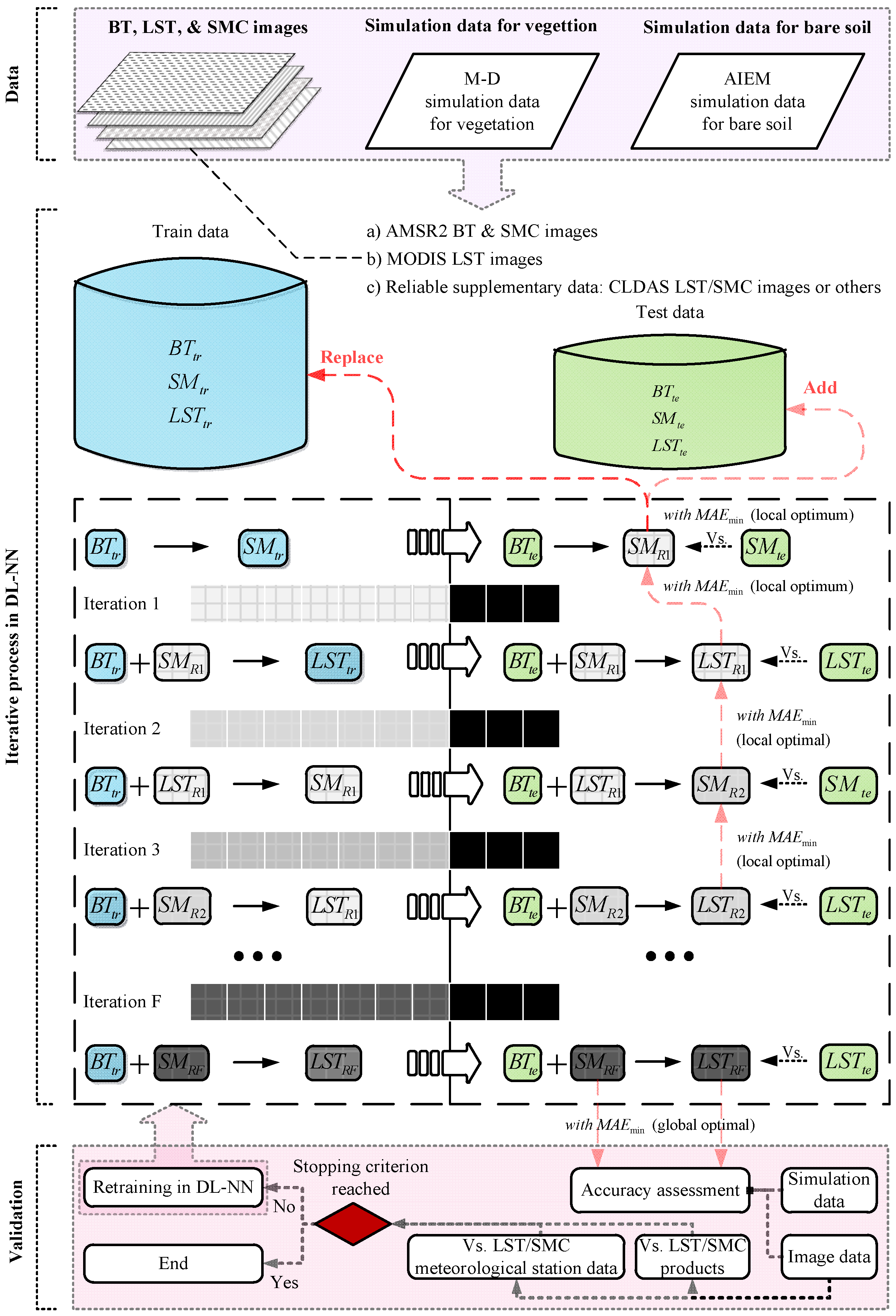
Figure 3 shows the developed iterative procedure for computing SM and LST. As can be seen, the training and test databases are continuously updated by the new retrievals. Iterations continue until the network structure reaches the global optimal solution, i.e., the difference between LST/SM estimates in two consecutive iterations is less than 0.01 K/0.001. In the figure, the subscripts
tr and
te indicate training data and test data respectively. The subscript in
Ri (
i = 1, 2, 3, …,
F) indicates the 𝑖th retrieved results, and
F represents the final iteration.
4. Results and Validation
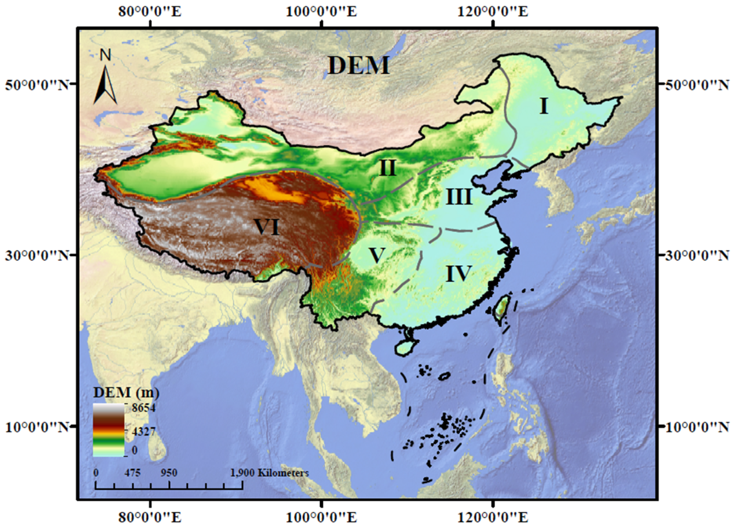
To verify the accuracy of the MDK-CR method, a case study in China was selected where we have more prior knowledge. China ranges from 3°31’00″ to 53°33’00″N latitude and 73°29’59″ to 135°2’30″E longitude. China’s terrain is high in the west and low in the east. The main terrain includes five types: plateau, mountain, hill, basin, and plain. Geographical location and diverse terrain determine China’s diverse climate, making the spatial distribution pattern of rainfall high in the southeast and low in the northwest. We selected the Chinese mainland as the research area because the climate types of different regions are distinct, and the Chinese mainland is divided into six regions according to the climate conditions (
Figure 4).
- (1)
SM retrieval
Considering that the most sensitive channel to SM retrieval is the low-frequency channel, we gradually reduced from fourteen channels to eight low-frequency channels. An introduction to deep learning methods and calculations can be found in [
25,
26,
54,
55]. The combination of different combination frequencies (eight to fourteen brightness temperature equations) is optimized by deep learning and the results are shown in
Table 1,
Table 2,
Table 3 and
Table 4.
As shown in the above tables, it can be concluded that the accuracy of SM retrieval of ten to fourteen channels is good and stable, and the minimum ME (mean absolute error) is about 0.037 m3/m3. However, the SM retrieval error of eight channels starts to become larger, which is not the best combination for SM retrieval. Further, considering the time cost and data redundancy, we recommend using ten low-frequency channels to retrieve SM, which can ensure high accuracy and efficiency.
- (2)
LST retrieval based on SM as a priori knowledge
Through geophysical logic reasoning, we know that soil moisture, as a priori knowledge, when used as input information for deep learning, can improve the accuracy of surface temperature retrieval. Therefore, the most accurate soil moisture value obtained by the above retrieval is used as prior knowledge to retrieve the surface temperature, together with the high-frequency brightness temperatures. Similar to the soil moisture retrieval above, we gradually reduce from fourteen channels and retain eight high-frequency channels. Through constant iteration, the LSTs retrieved based on SM as priori knowledge are shown in
Table 5,
Table 6,
Table 7 and
Table 8, and the accuracy is relatively stable.
As shown in the above tables, it can be concluded that the accuracy of LST retrieval of ten to fourteen channels is good and stable, and the minimum ME is about 1.5 K. However, the LST retrieval error of eight channels starts to become larger, i.e., it is not the best combination for LST retrieval. Similar to soil moisture retrieval, we recommend using soil moisture as prior knowledge and ten high-frequency channels to retrieve LST, which can ensure high accuracy and efficiency.
- (3)
Iterative retrieval based on LST and SM as a priori knowledge
We continue to use the LST dataset with the highest accuracy retrieved above as a priori knowledge, and we use ten low-frequency brightness temperatures as input nodes for deep learning to retrieve SM. We then use the highest SM value obtained from previous retrieval as a priori knowledge and high-frequency brightness temperature as input information to retrieve LST. After three iterations, the SM and LST retrieved based on LST or SM as priori knowledge are shown in
Table 9 and
Table 10. The minimum average error is about 0.027 m
3/m
3, which is 0.01 m
3/m
3 higher than without prior knowledge (LST). The highest average accuracy for the retrieval of surface temperature is 1.38 K, which is 0.12 K higher than the first inversion. Although we continued to iterate, which made the inversion more stable, the average accuracy was not improved further. The accuracy of deep learning training and testing has a close relationship with the accuracy of the collected training and test datasets. If we want to further improve the accuracy, we need to further discriminate the sample accuracy of the training and test data or add a more high-precision data set. We can also build different training and testing databases according to different regions, seasons, and weather conditions, so as to improve the accuracy of the retrieval.
- (4)
Validation and application
(1) A case study.
To provide an example of the application of the algorithm, the images of AMSR2 in China on 20 July 2019 were selected as a case study. Using the training database established above, we input the brightness temperatures accordingly, and iteratively calculate SM and LST.
Figure 5A,B shows that the distribution trend of retrieved SM in China is relatively reasonable, and the retrieval results are consistent with the distribution of dry and wet conditions in north and south China. The SM gradually increases from northwest to southeast China. The overall performance is the “western dry, northeastern and southeastern wet” spatial distribution pattern. The ascending orbit (
Figure 5A) shows the daytime (13:30) and the descending orbit (
Figure 5B) shows the nighttime (1:30). In general, SM at night is higher than SM during the day. SM with a low value is mainly distributed in the desert from the Tarim Basin to the Alashan Plateau in Xinjiang, Gobi (in the Ⅱ area, Northwest China). The average SM is below 0.1 m
3/m
3. These areas have temperate continental climates with less precipitation and strong radiation, and the surface water fixation capacity is poor due to low vegetation coverage. The SM with high value is mainly distributed in the Northeast Plain (Ⅰ area) and North China Plain (Ⅲ area). In the plains, the Yangtze River Basin, and south of the Yangtze River, the average SM is more than 0.3 m
3/m
3. These areas are mostly affected by monsoon climates, high temperature and rain in summer, high vegetation coverage, developed water systems, and good surface water fixation capacities.
Figure 5a,b are the corresponding AMSR2 soil moisture products obtained from the Japan Aerospace Exploration Agency (JAXA). By comparing
Figure 5A,a,B,b, we see that the soil moisture results retrieved by the MDK-CR method are in good agreement with the overall trend of AMSR2 soil moisture products. In northeast and southwest China, there are many forest cover areas, and the soil moisture product of AMSR2 is somewhat overestimated. Soil moisture under forests is usually not too high, and ground observatory data have confirmed this observation [
39,
40]. The soil moisture retrieved by the MDK-CR method is more reasonable than the official product.
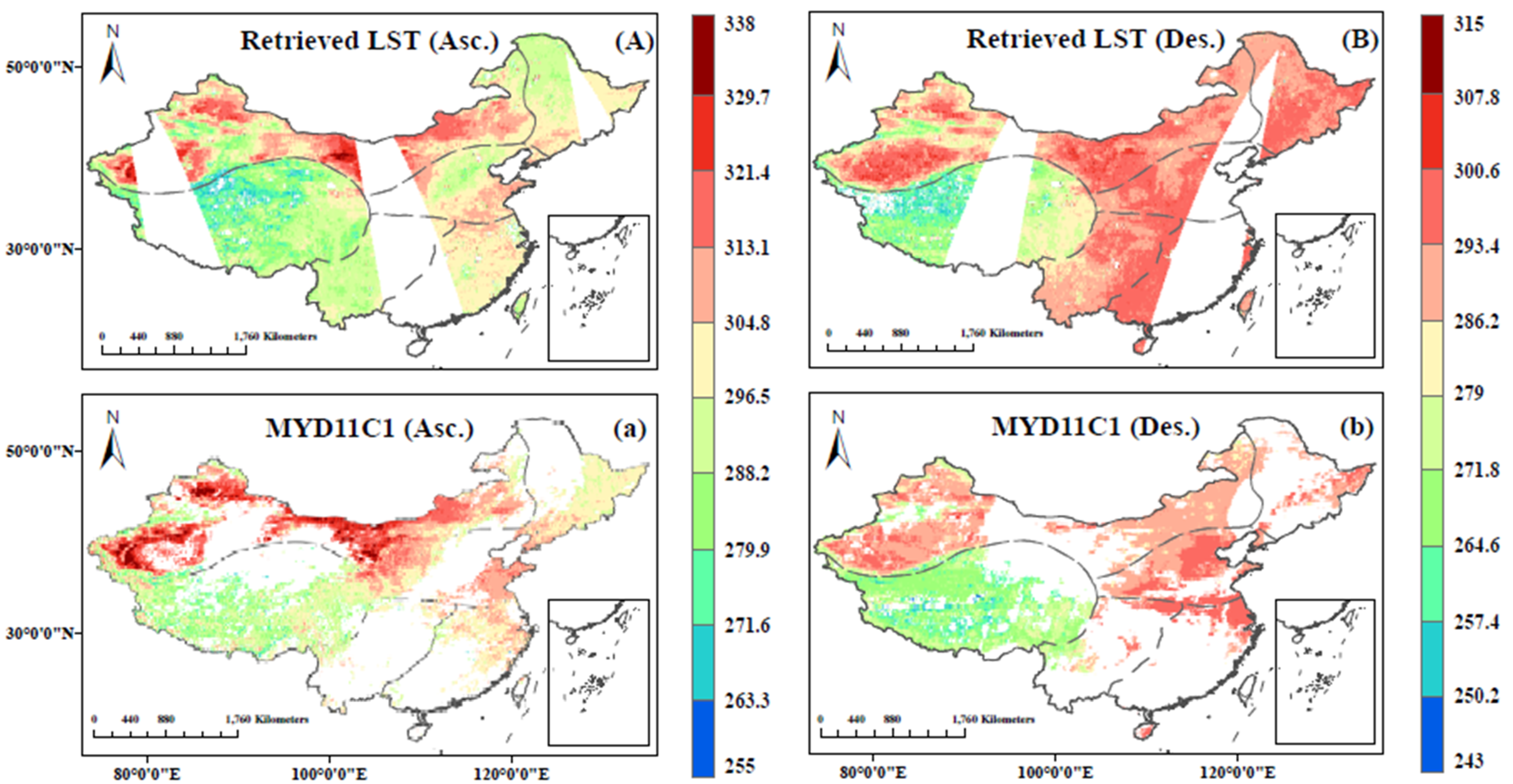
Figure 6A is the retrieval LST of the MDK-CR method during the day (13:30), which shows that the distribution trend of LST in China is relatively reasonable. The LST of the Badain Jaran Desert, Tengger Desert, and Taklimakan Desert in Xinjiang is the highest, and the LST of the Qinghai-Tibet Plateau is the lowest. Under normal circumstances, the surface temperature in northern China is lower than that in southern China, but the daytime temperature retrieval results on this day are just the opposite. The main reason is that southern China is covered by clouds, which leads to the inability of thermal infrared remote sensing to retrieve the surface temperature, as can be seen from the corresponding MODIS LST product data (
Figure 6a). There are no clouds in the sky of northern China, and the sun’s rays shine directly on the ground surface, resulting in relatively high surface temperatures in northern China. There are relatively few clouds in northern China, and the ground heat dissipation is very fast. The south of China is cloudy and has good thermal insulation effect. As a result, the nighttime temperature in southern China is relatively high, as shown in
Figure 6B,b. By comparing
Figure 6A,a,B,b, we find that the LST results retrieved by the MDK-CR method are in good agreement with the overall trend of MODIS LST products under cloud-free conditions. When there are clouds in the sky, we can use passive microwave remote sensing data to retrieve surface temperature, which has unique advantages by comparison.
(2) Validation.
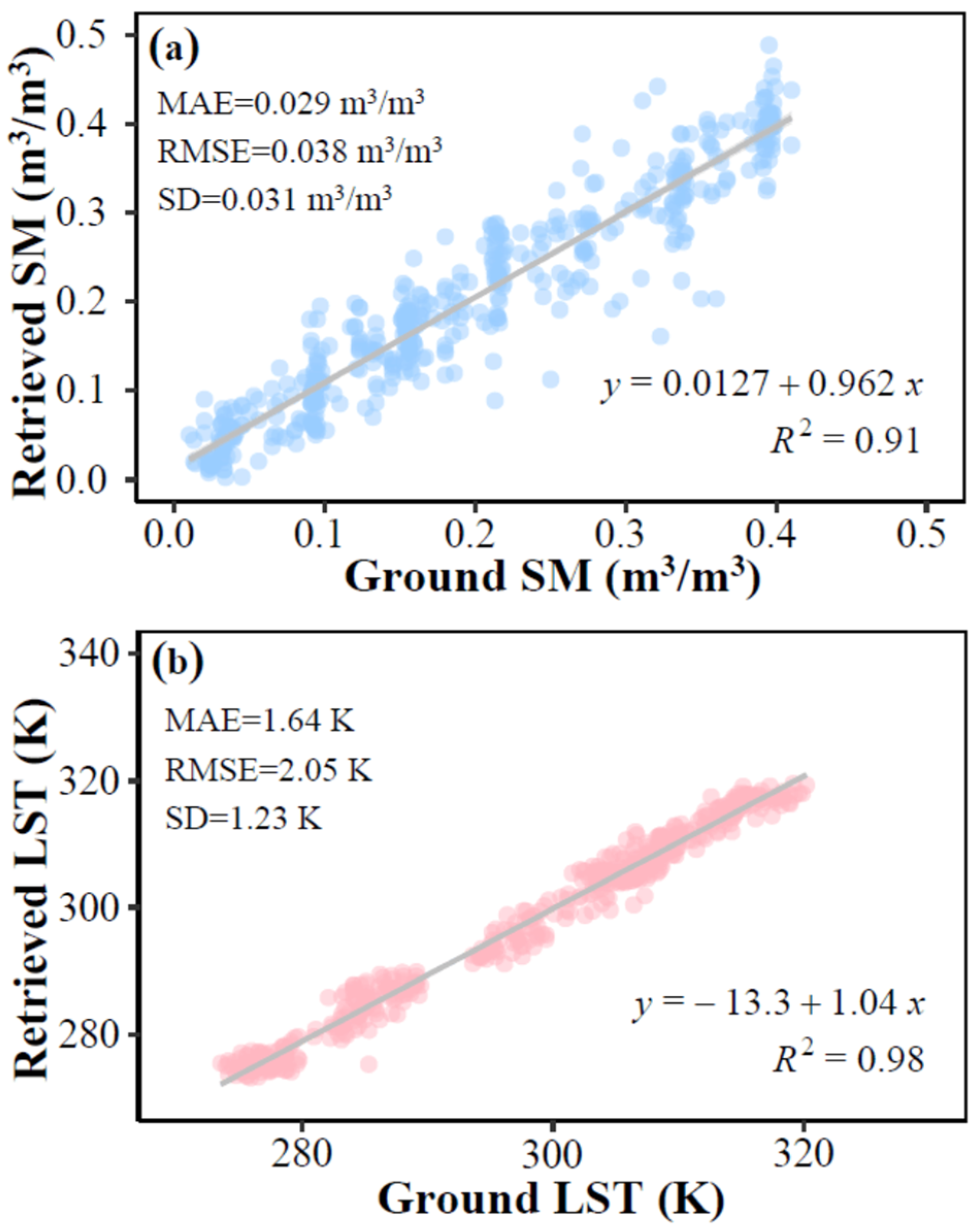
Ground validation is very important for the practical application and promotion of the method. Although the ground point measured data and the large-scale remote sensing retrieval results cannot be accurately docked on the spatial scale of expression, we used multi-source surface temperature data to ensure the accuracy of ground temperature as much as possible. To ensure the accuracy of data collection, only these data were used when soil moisture and LST values from ground observation sites were very close to both the ERA5 and CLDAS data. We selected eighteen observation sites with flat terrain and relatively single surface type in China, and we extracted a total of 495 observation data sets from 2018 to 2019. The retrieved result pixel is extracted according to the latitude and longitude position of the observation station. As shown in
Figure 7a, the mean absolute error (MAE) of the retrieved SM and ground synchronization observation data was 0.029 m
3/m
3, and the RMSE was 0.037 m
3/m
3, and the coefficient of determination (R
2) was 0.91. As seen in
Figure 7b, the MAE of the retrieved LST and ground synchronization observation data was 1.64 K, the RMSE was 2.05 K, and the R
2 was 0.98.
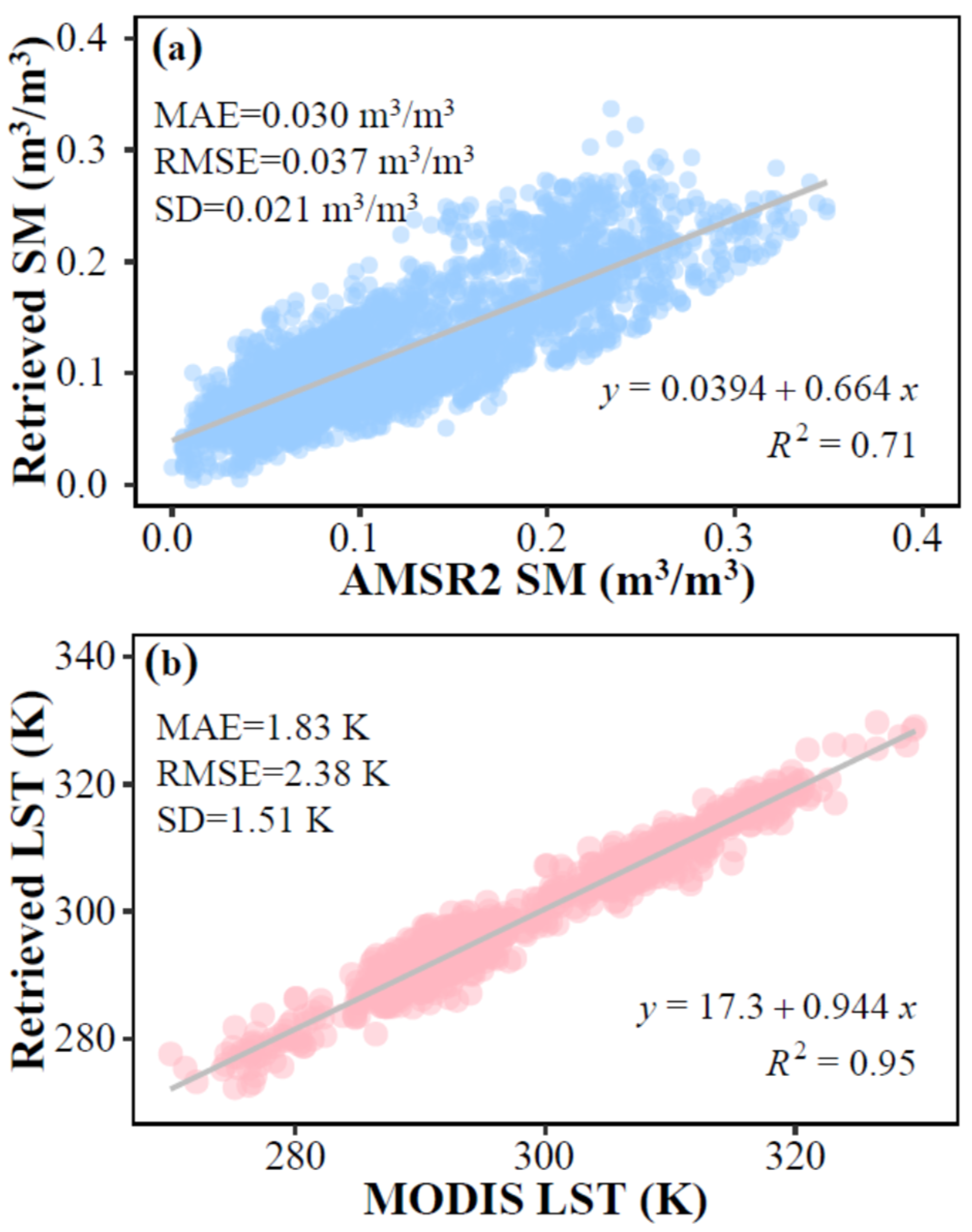
Cross-validation is also an important part of comparing the algorithm with similar products before its application. We compared the retrieved SM and LST with the SM products of AMSR2 and the LST products of MODIS, respectively. Spatial comparisons between different products have been made in
Figure 5 and
Figure 6, and the comparative analysis found that the overall situation of the spatial contrast was very good. Specifically, after resampling
Figure 5 and
Figure 6to the same resolution, we conducted random sampling in different areas where both had effective values. There are 2862 samples of soil moisture and 1653 samples of surface temperature, and cross validation is shown in
Figure 8. Taking the soil moisture product of AMSR2 as a reference, the MAE of soil moisture estimated by the MDK-CR method was 0.03 m
3/m
3 and RMSE was 0.037 m
3/m
3. Compared with MODIS LST (MYD11C1) products, the MAE of LST estimated by the MDK-CR method was 1.83 K and the RMSE was 2.38 K. Comparative analysis showed that our algorithm has high consistency with other algorithm products, and our algorithm has certain advantages because it can adapt to more situations by supplementing high-precision samples.


 ,
, 


