
Exploring the Relationships between Land Surface Temperature and Its Influencing Factors Using Multisource Spatial Big Data: A Case Study in Beijing, China


Abstract
:1. Introduction
2. Literature Review
2.1. Urban Heat Island Effect and Land Surface Temperature
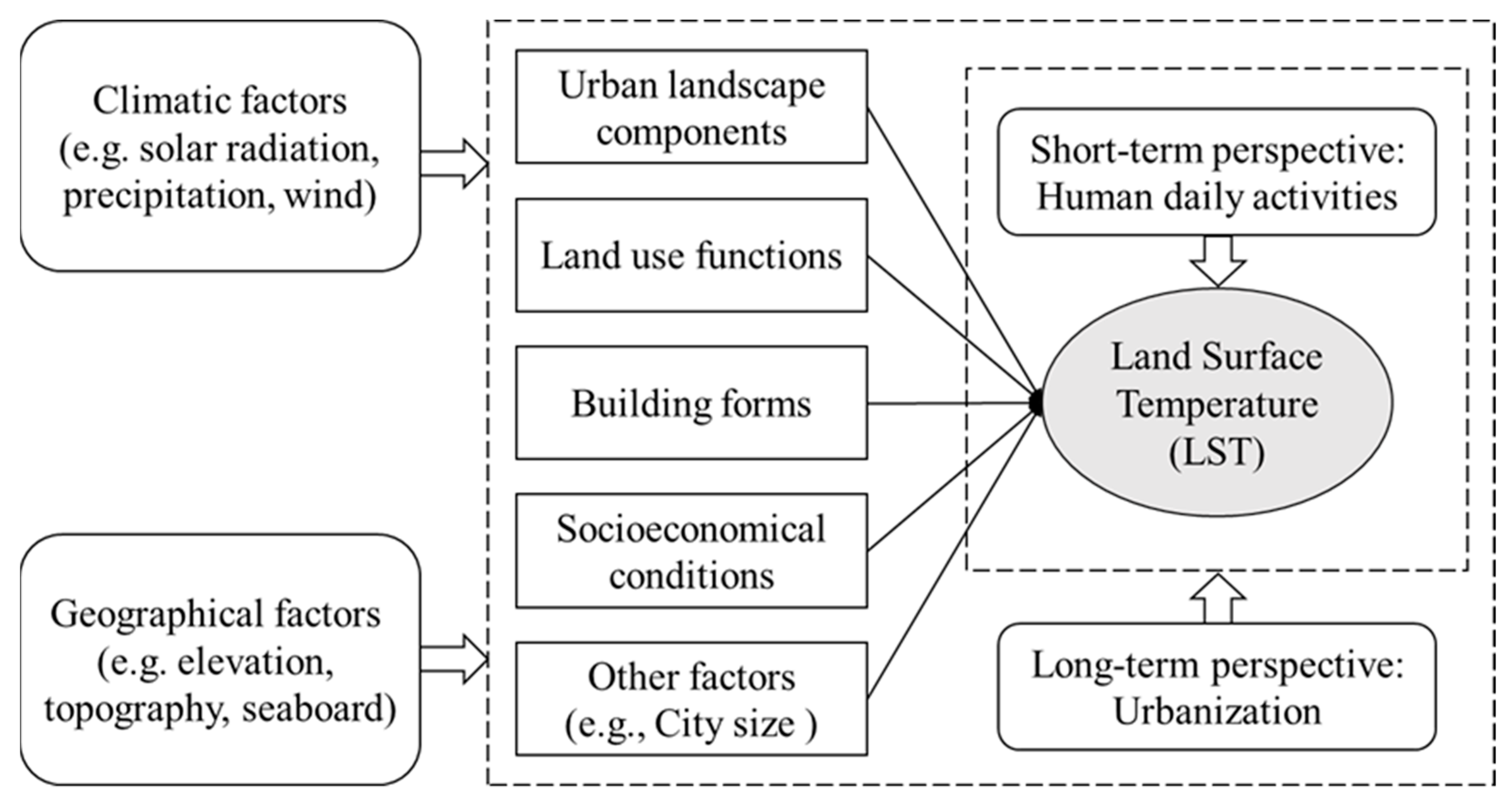
2.2. Influencing Factors of Land Surface Temperature
3. Data and Methods
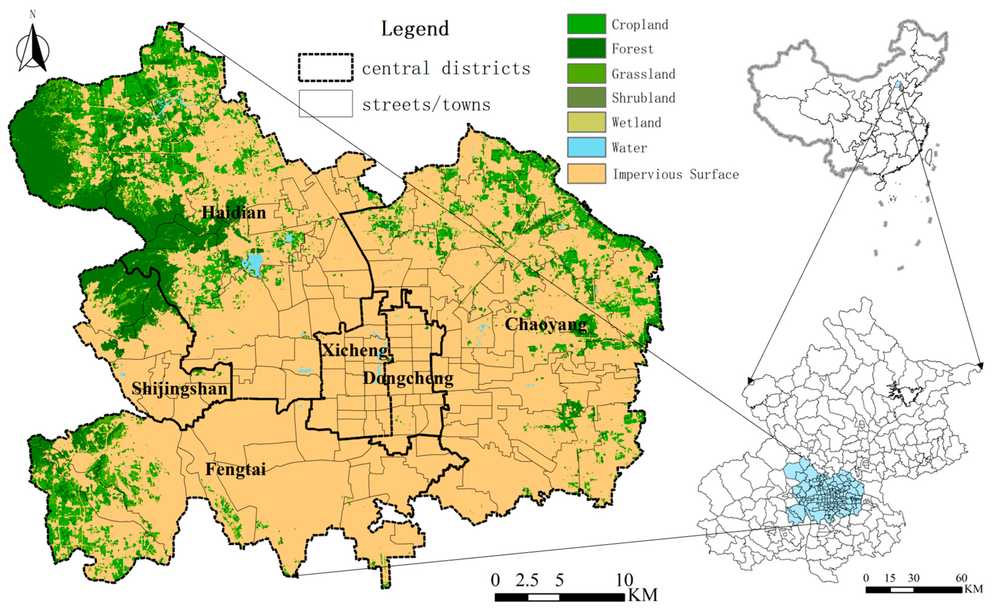
3.1. Study Area
3.2. MODIS Data for LST
3.3. Spatial Big Data to Account for Human Activities
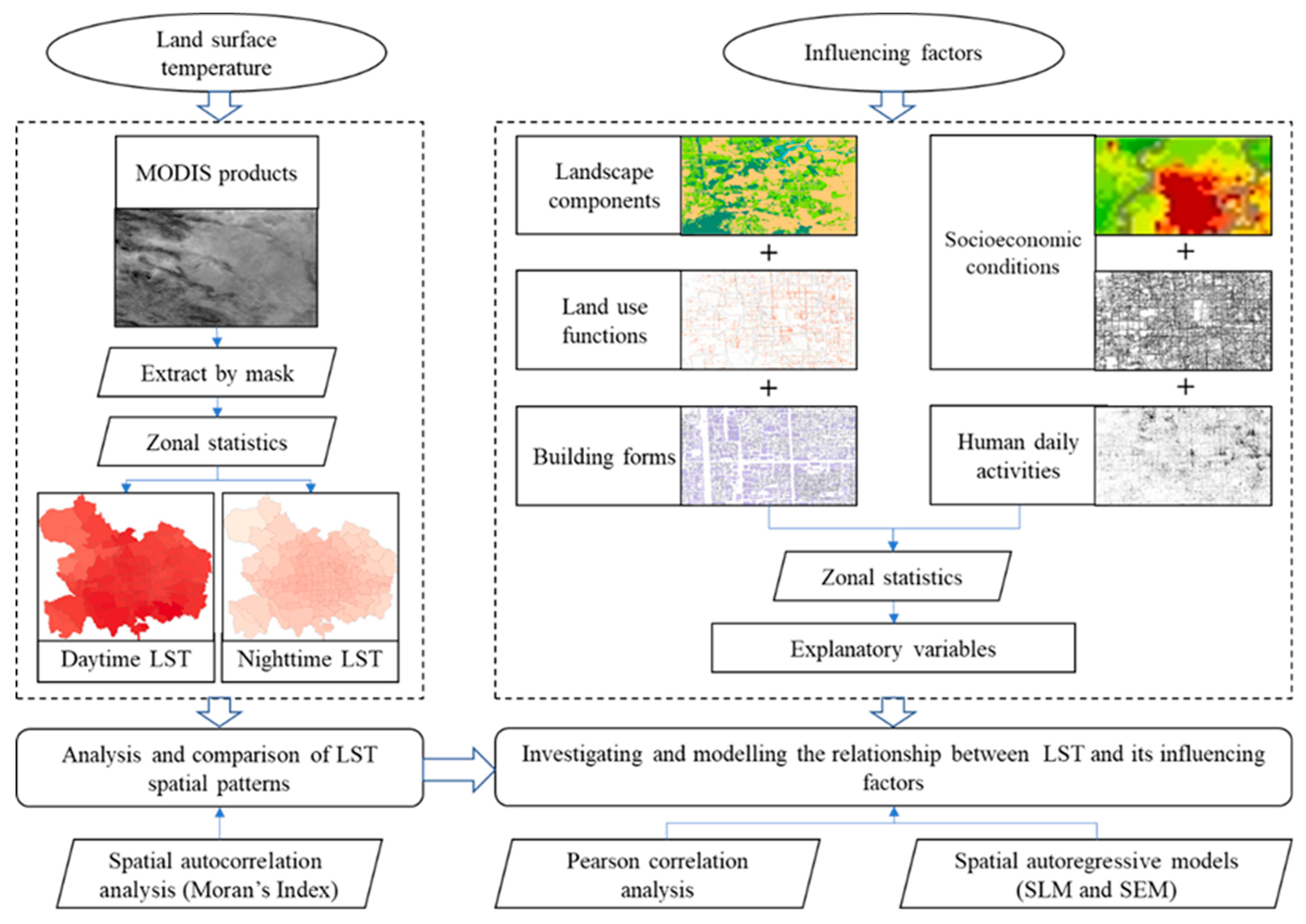
3.4. Methods
4. Results
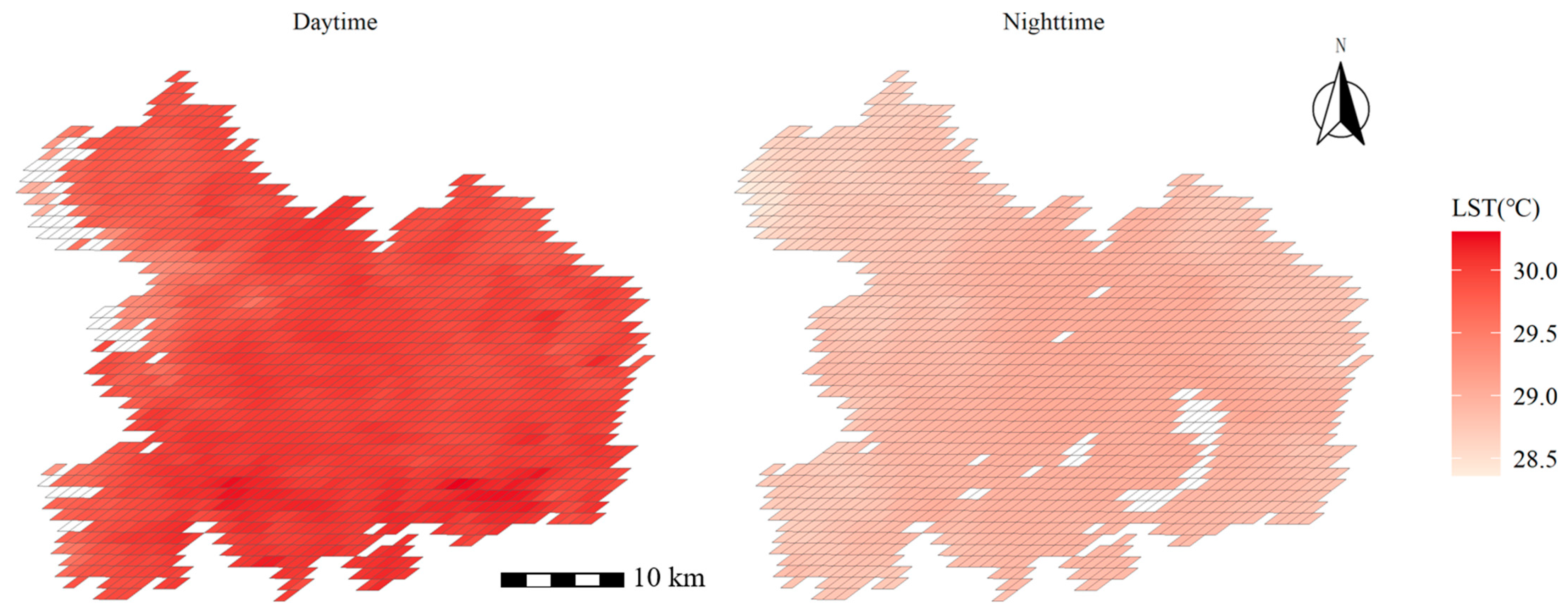
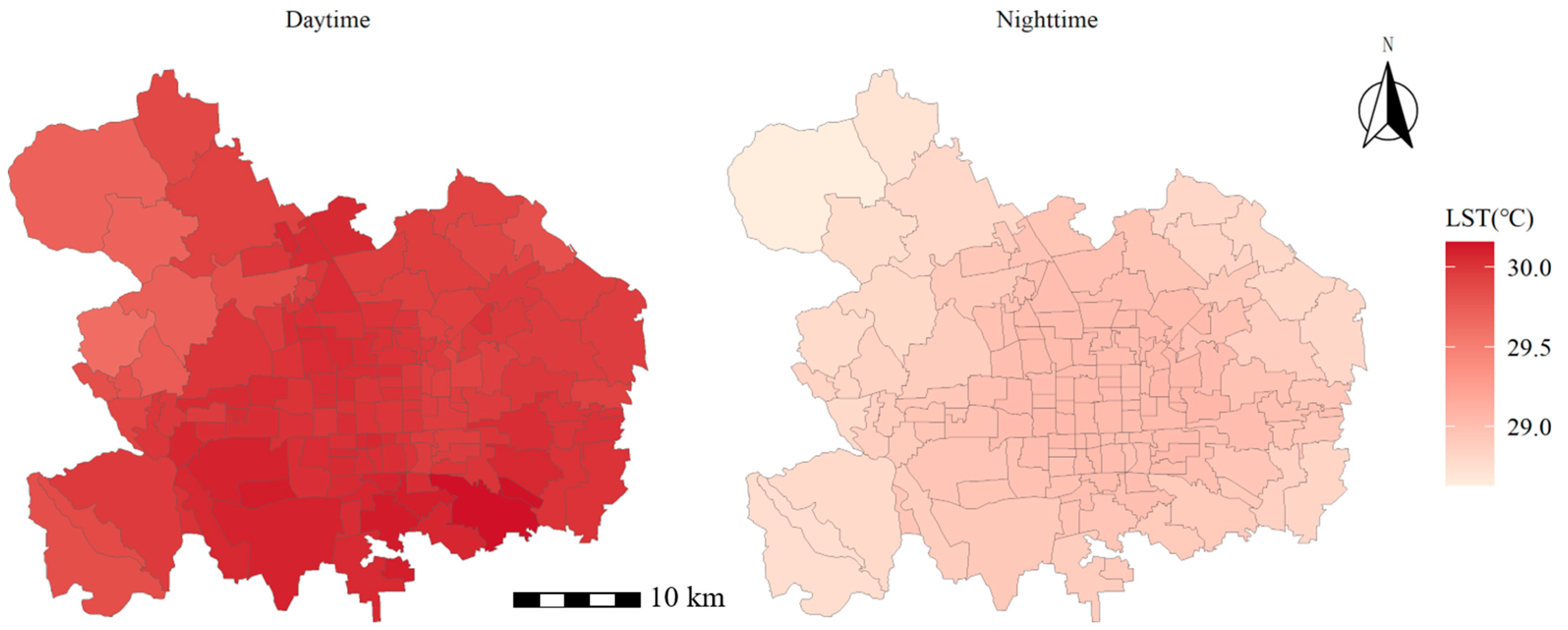
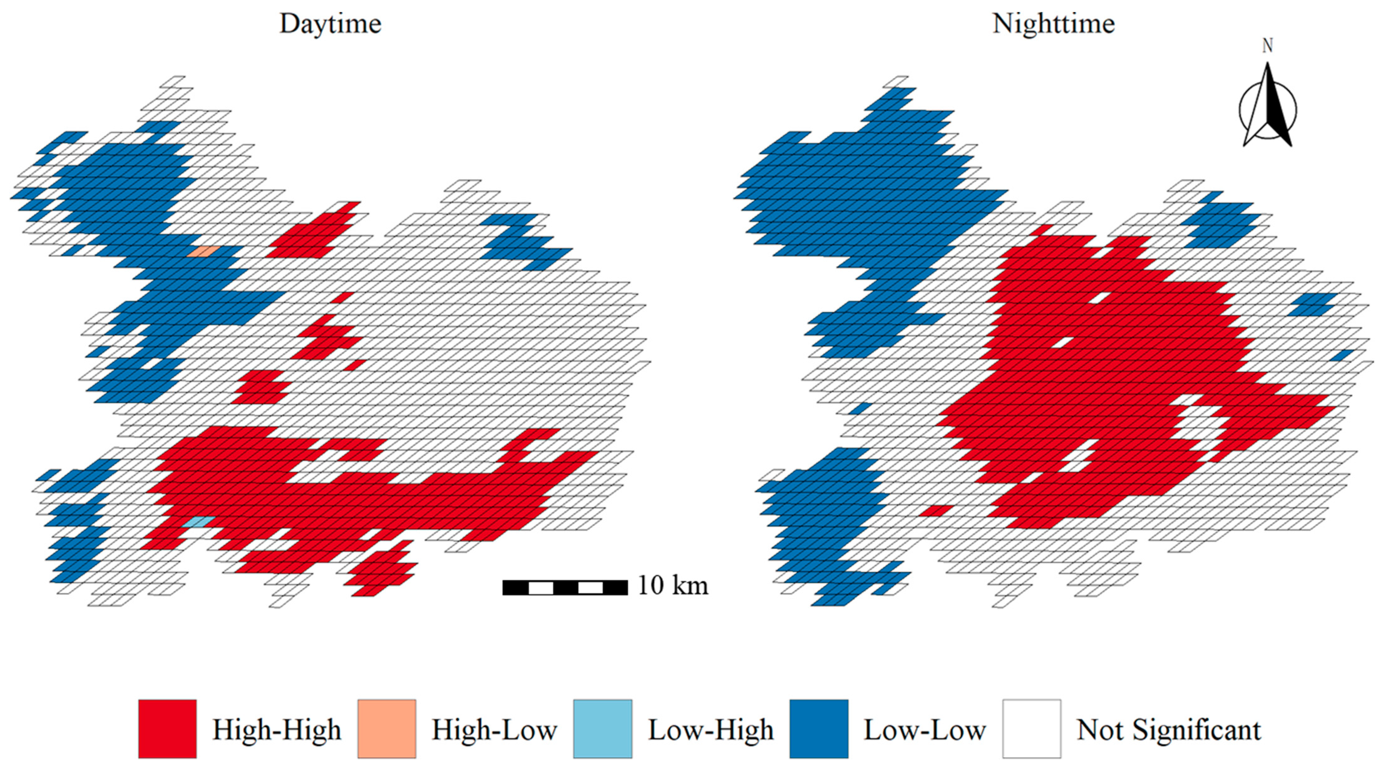
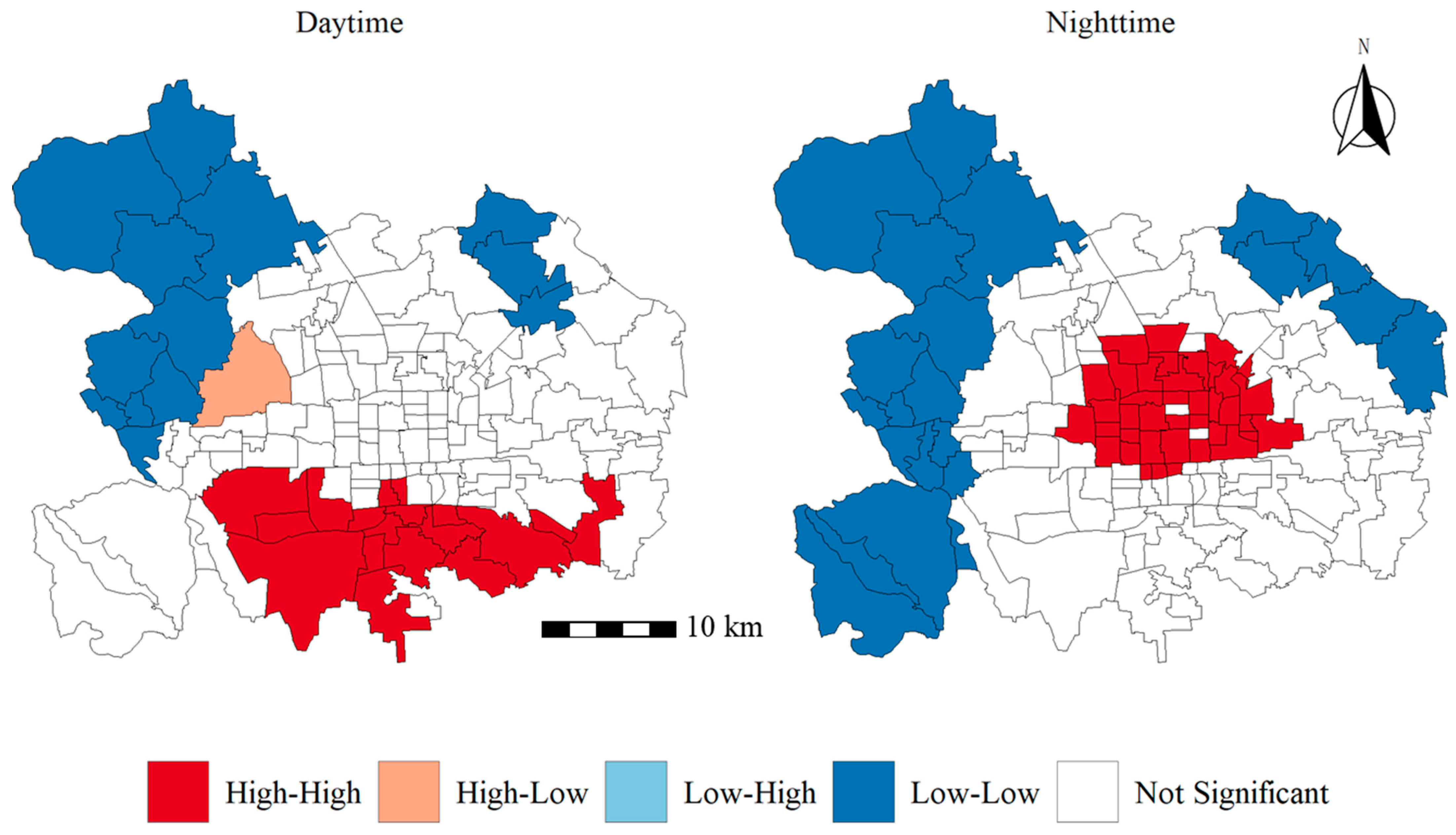
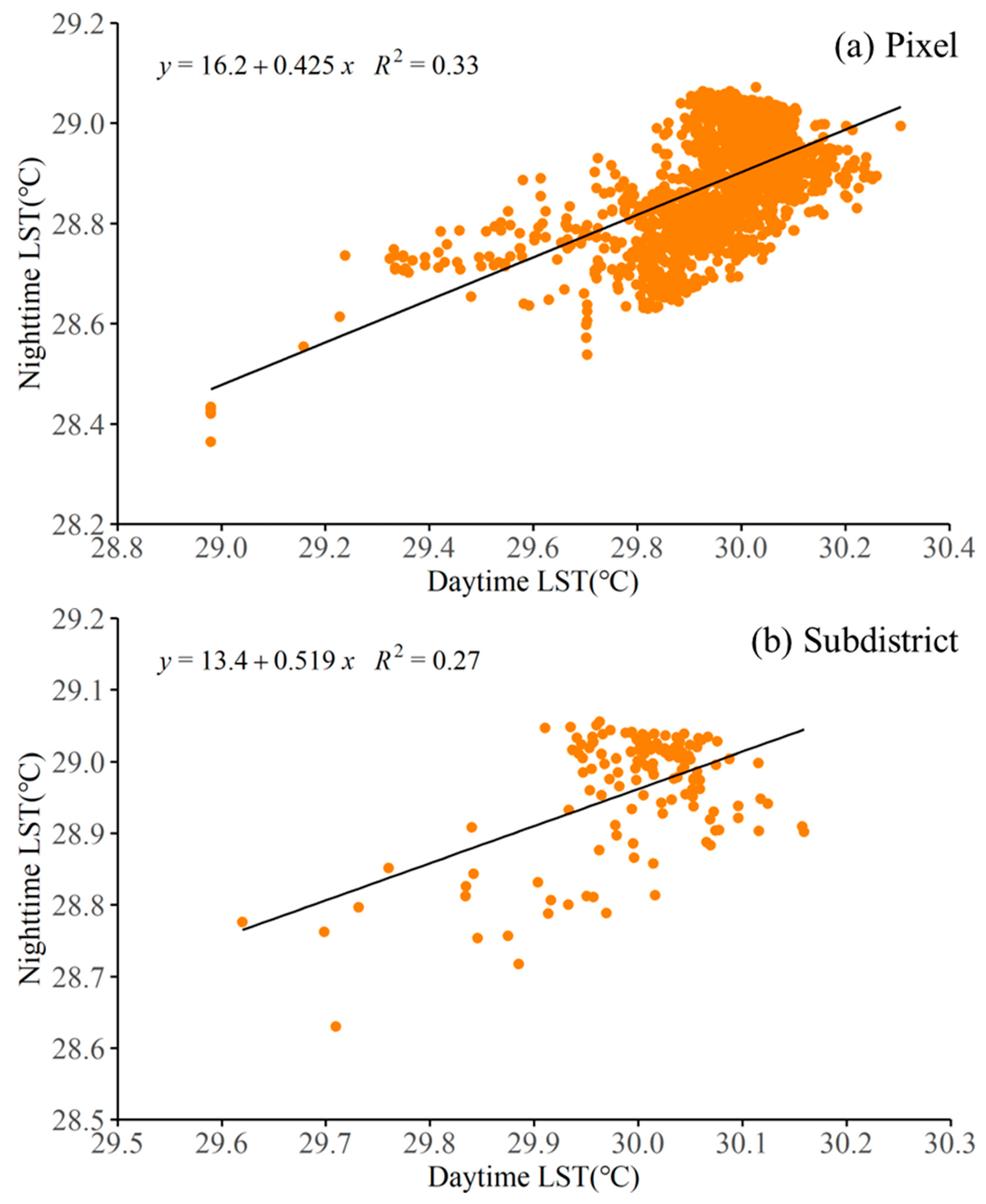
4.1. Spatiotemporal Patterns of LST
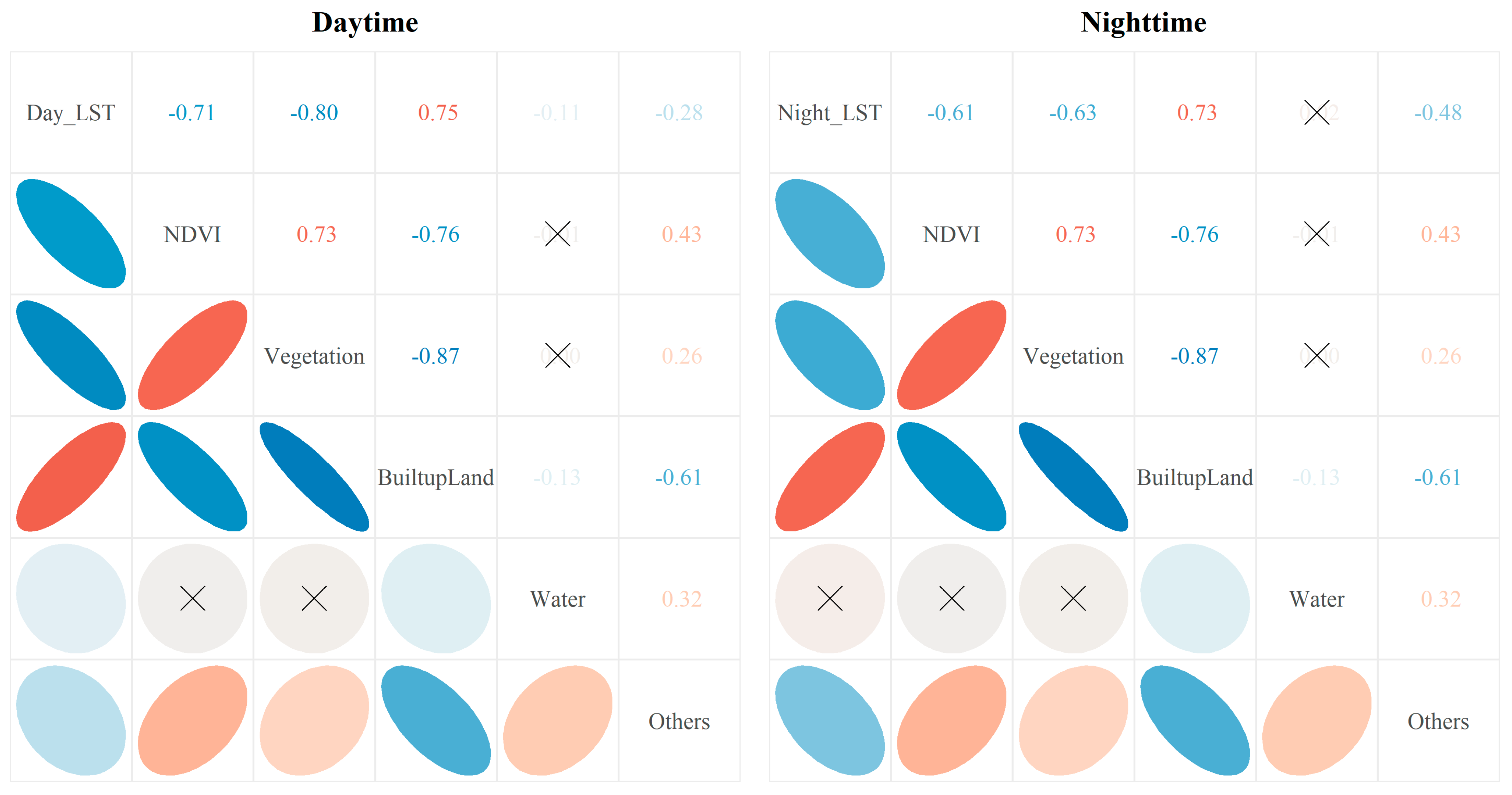
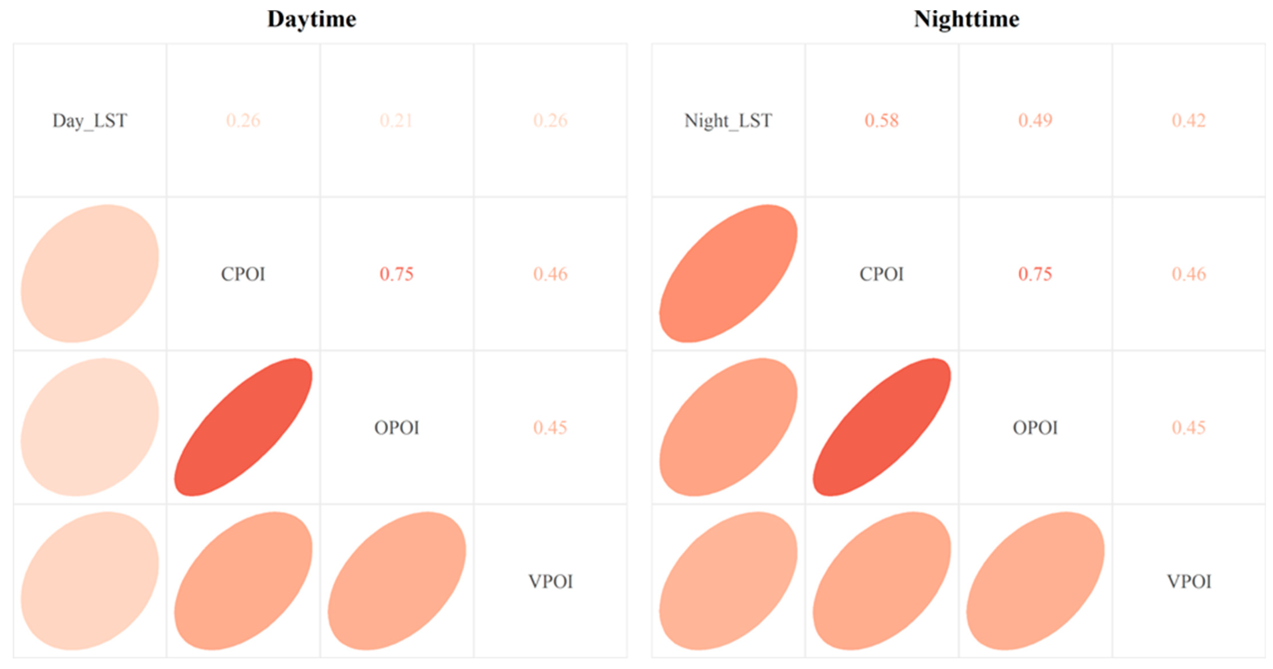
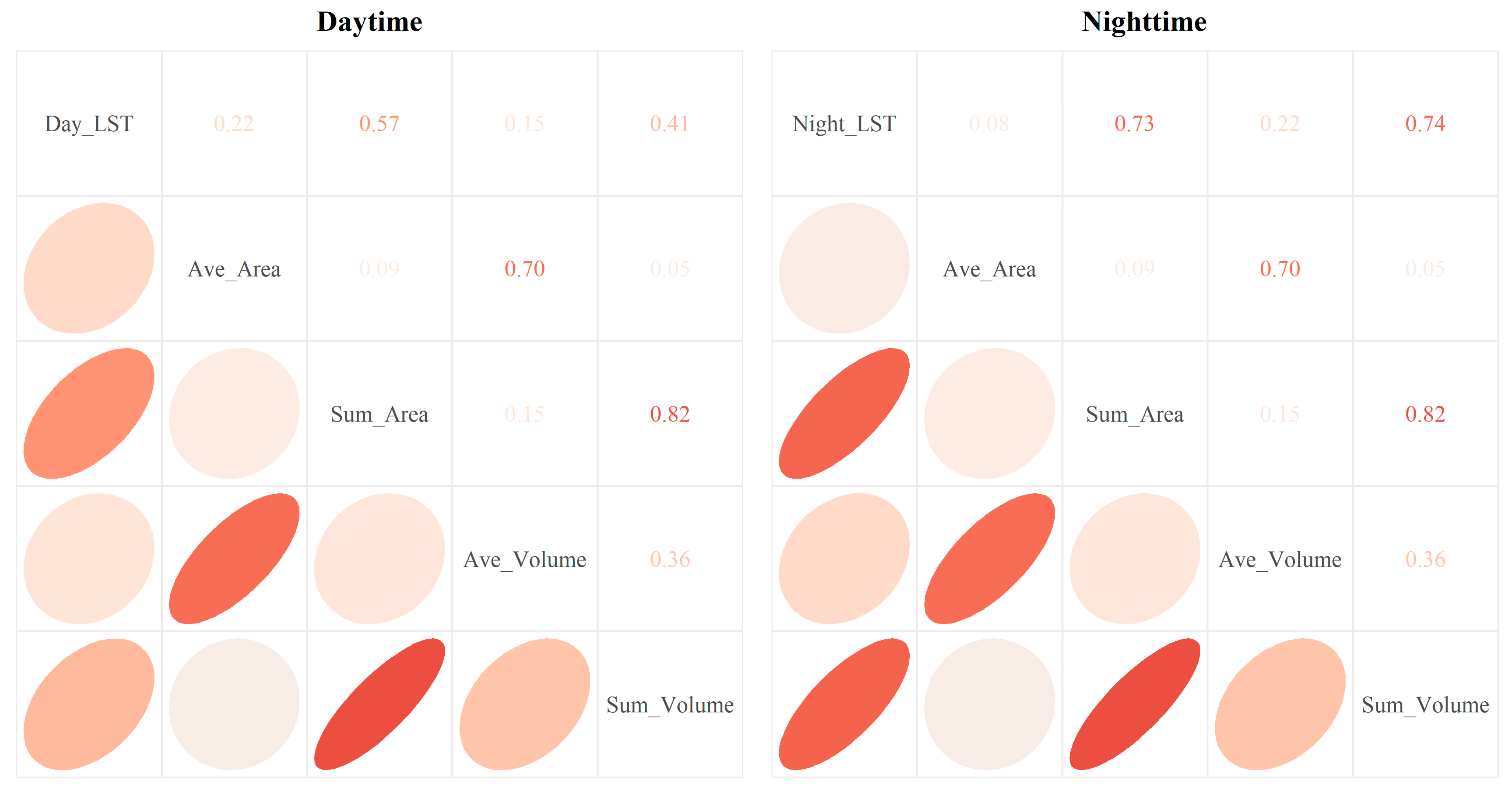
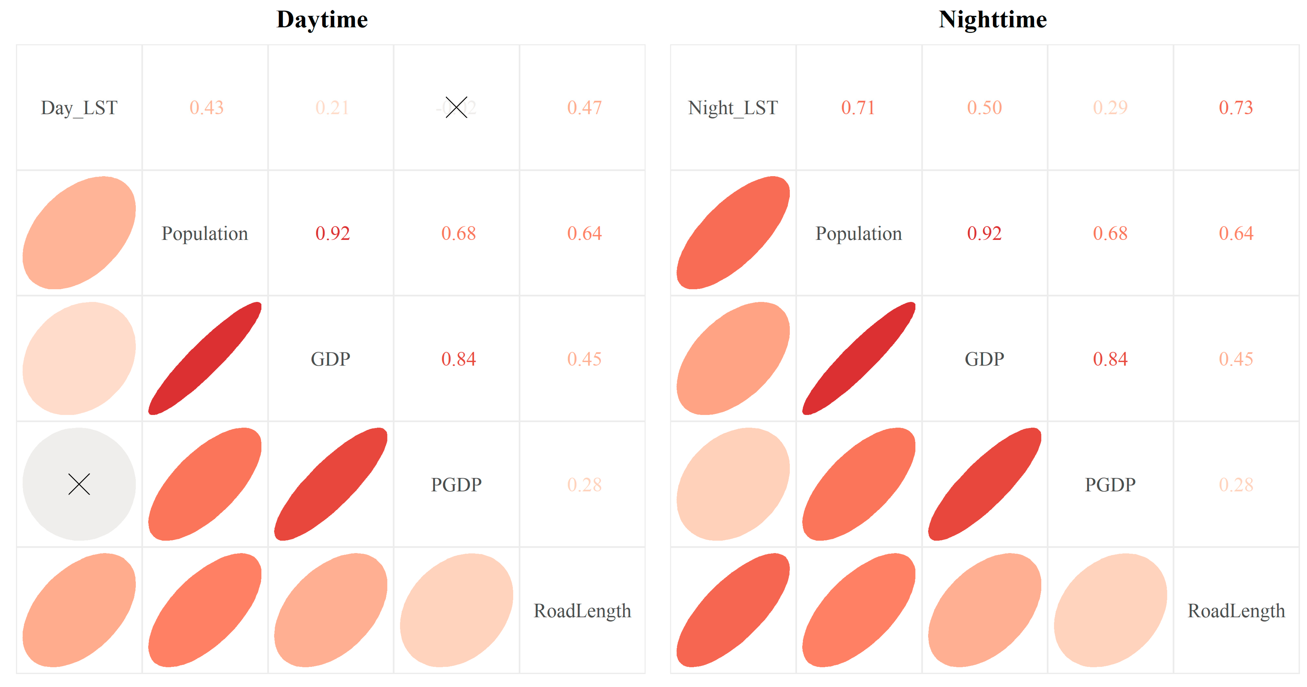
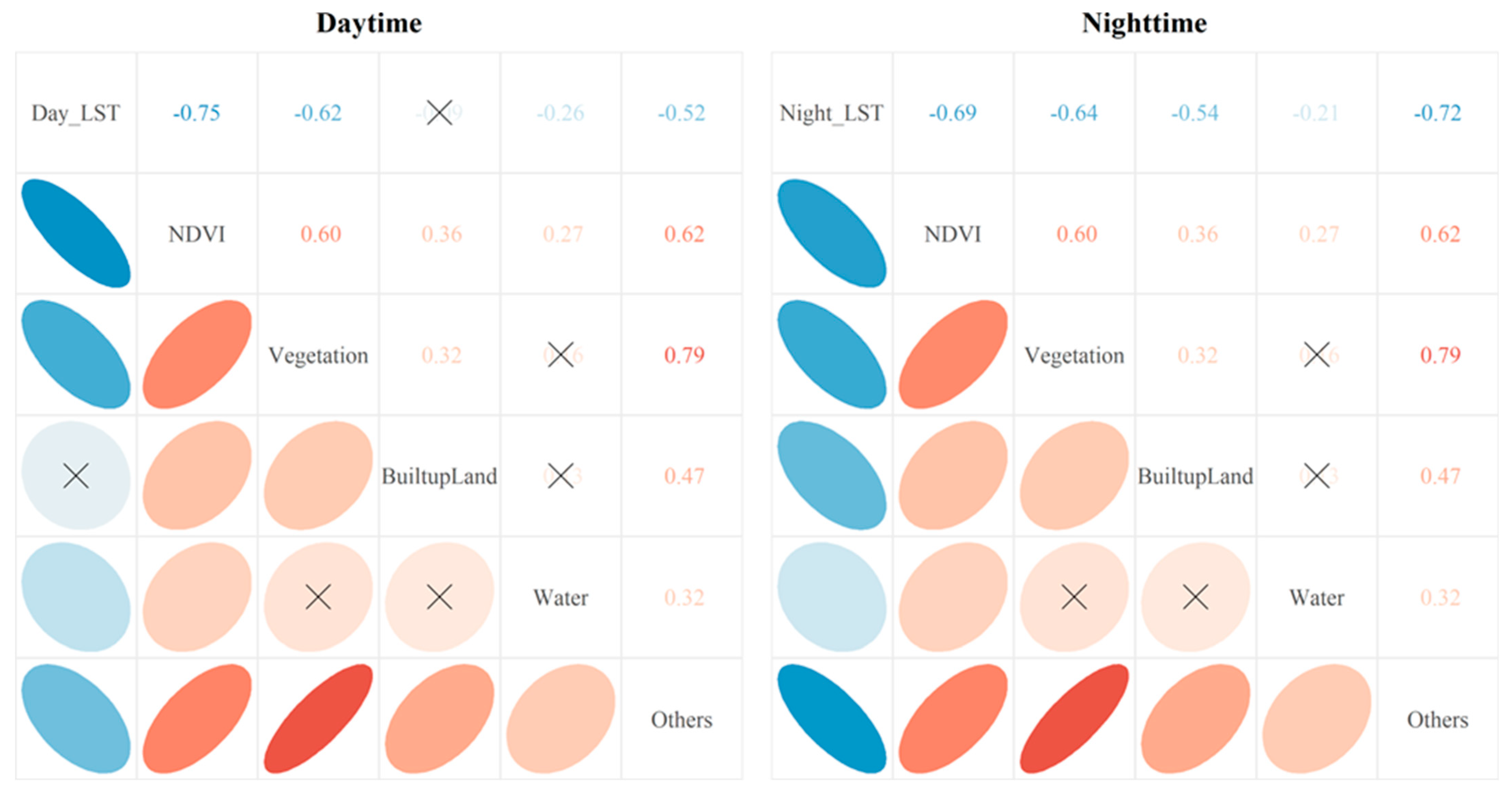
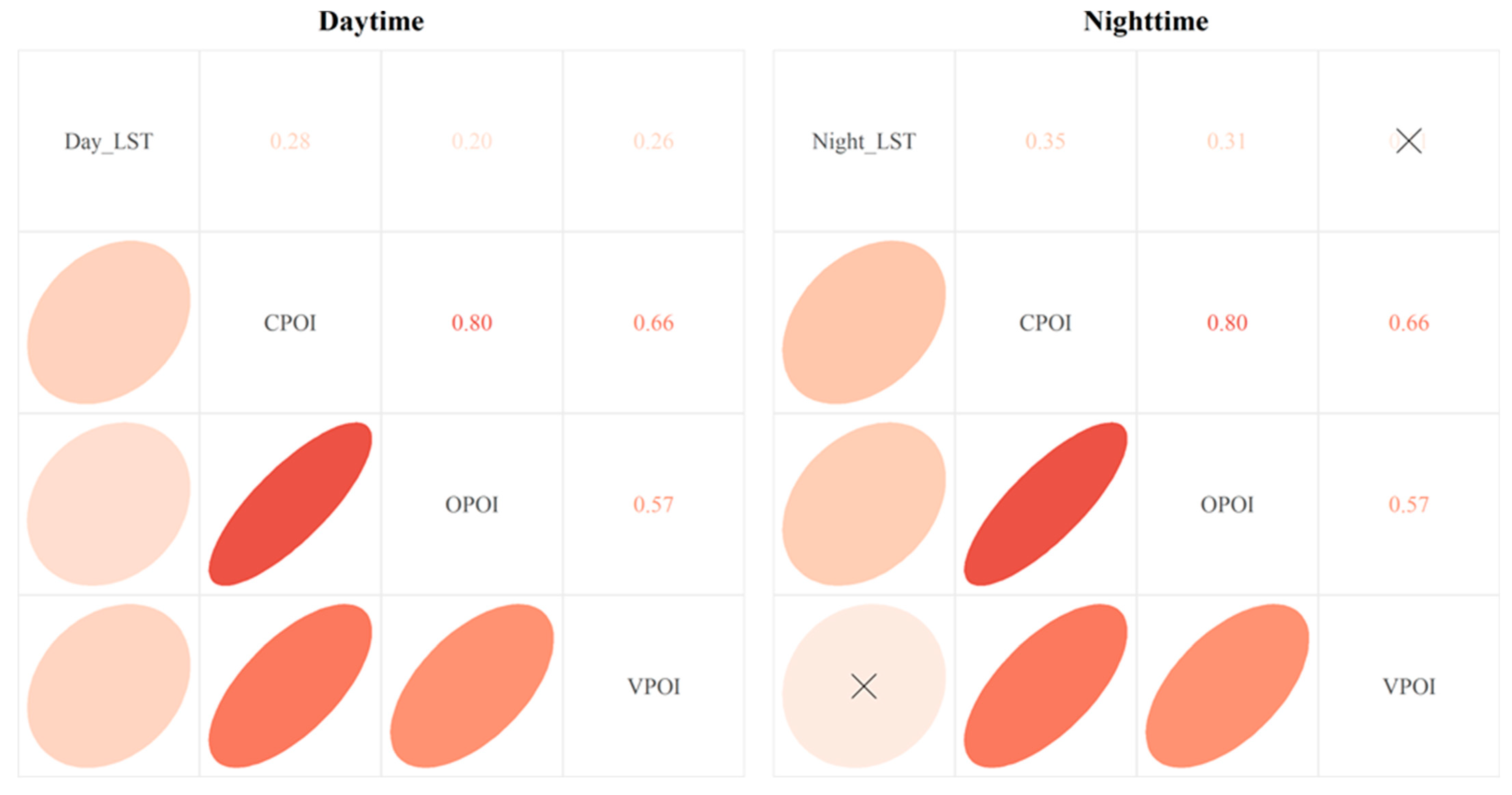
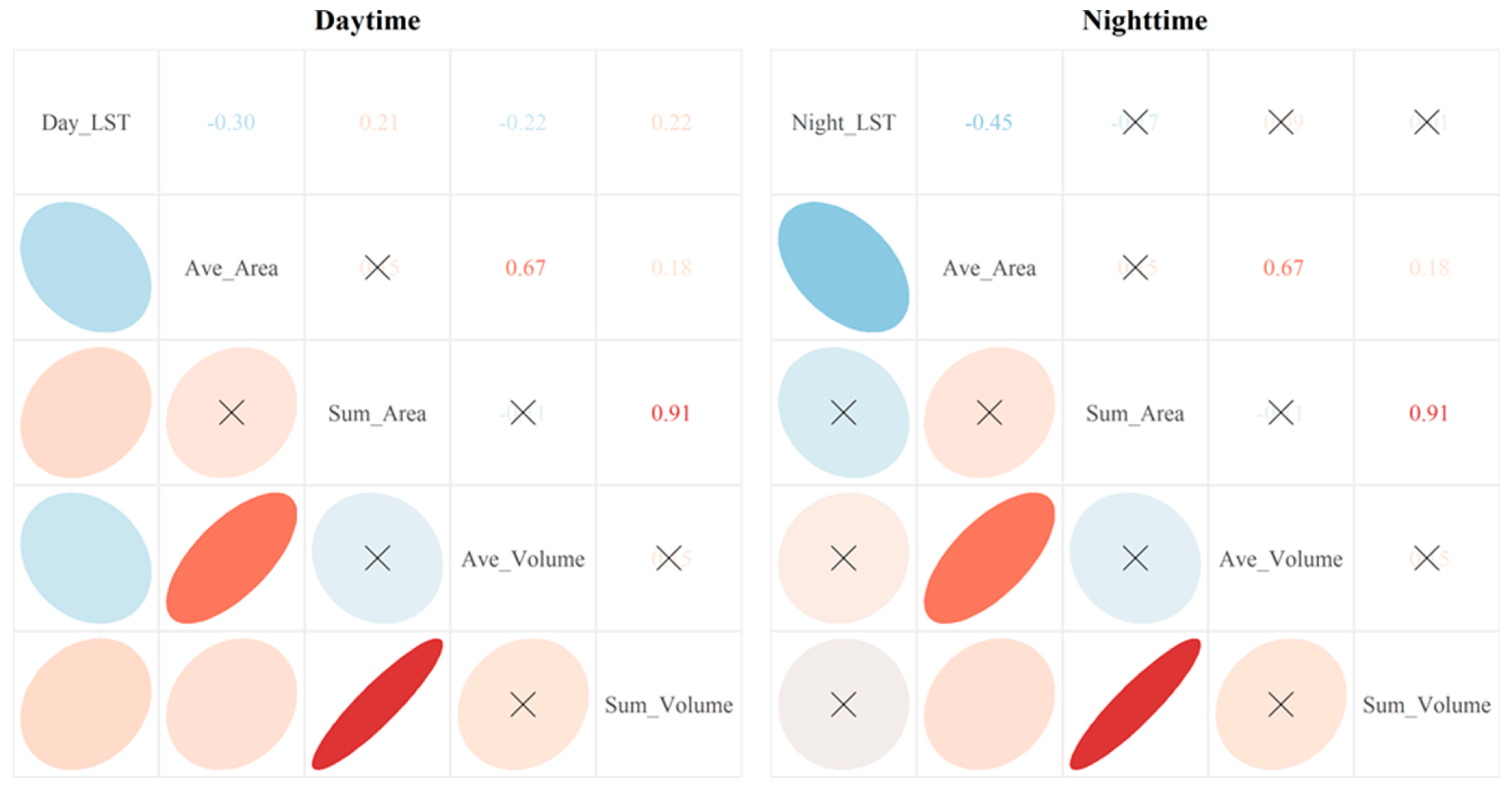
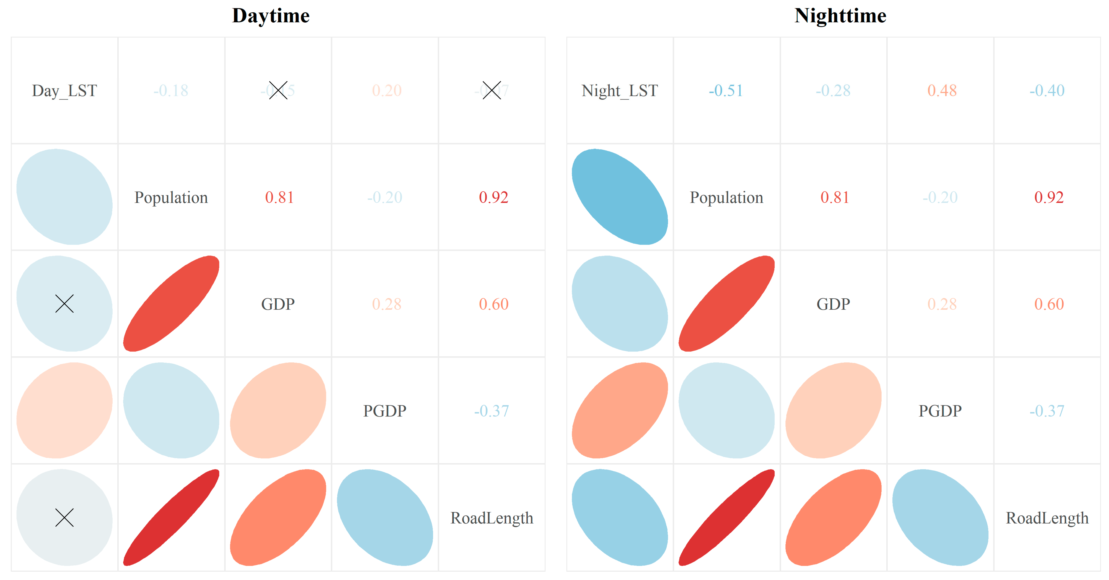
4.2. Results of Pearson Correlation Analysis
4.3. Results of Empirical Regressions
5. Discussion
5.1. Implications for Urban Sustainable Development
5.2. Limitation and Future Work
6. Conclusions
Author Contributions
Funding
Data Availability Statement
Acknowledgments
Conflicts of Interest
References
- Shah, P.B.; Patel, C.R. Integration of Remote Sensing and Big Data to Study Spatial Distribution of Urban Heat Island for Cities with Different Terrain. Int. J. Eng. 2023, 36, 71–77. [Google Scholar] [CrossRef]
- Oroud, I.M. Integration of GIS and remote sensing to derive spatially continuous thermal comfort and degree days across the populated areas in Jordan. Int. J. Biometeorol. 2022, 66, 2273–2285. [Google Scholar] [CrossRef] [PubMed]
- Heaviside, C. Urban Heat Islands and Their Associated Impacts on Health. In Oxford Research Encyclopedia of Environmental Science; Oxford University Press: Oxford, UK, 2020. [Google Scholar]
- Oke, T.R. City size and the urban heat island. Atmos. Environ. 1973, 7, 769–779. [Google Scholar] [CrossRef]
- Oke, T.R. The Heat Island of the Urban Boundary Layer: Characteristics, Causes and Effects. In Wind Climate in Cities; Cermak, J.E., Davenport, A.G., Plate, E.J., Viegas, D.X., Eds.; Springer: Dordrecht, The Netherlands, 1995; pp. 81–107. [Google Scholar]
- Zhou, B.; Rybski, D.; Kropp, J.P. The role of city size and urban form in the surface urban heat island. Sci. Rep. 2017, 7, 4791. [Google Scholar] [CrossRef] [Green Version]
- Maimaitiyiming, M.; Ghulam, A.; Tiyip, T.; Pla, F.; Latorre-Carmona, P.; Halik, U.; Sawut, M.; Caetano, M. Effects of green space spatial pattern on land surface temperature: Implications for sustainable urban planning and climate change adaptation. Isprs J. Photogramm. Remote Sens. 2014, 89, 59–66. [Google Scholar] [CrossRef] [Green Version]
- Rao, Y.X.; Dai, J.Y.; Dai, D.Y.; He, Q.S. Effect of urban growth pattern on land surface temperature in China: A multi-scale landscape analysis of 338 cities. Land Use Policy 2021, 103, 105314. [Google Scholar] [CrossRef]
- Heaviside, C.; Macintyre, H.; Vardoulakis, S. The Urban Heat Island: Implications for Health in a Changing Environment. Curr. Environ. Health Rep. 2017, 4, 296–305. [Google Scholar] [CrossRef] [PubMed]
- Li, X.; Zhou, Y.; Yu, S.; Jia, G.; Li, H.; Li, W. Urban heat island impacts on building energy consumption: A review of approaches and findings. Energy 2019, 174, 407–419. [Google Scholar] [CrossRef]
- Simwanda, M.; Murayama, Y. Spatiotemporal patterns of urban land use change in the rapidly growing city of Lusaka, Zambia: Implications for sustainable urban development. Sustain. Cities Soc. 2018, 39, 262–274. [Google Scholar] [CrossRef]
- Heinl, M.; Hammerle, A.; Tappeiner, U.; Leitinger, G. Determinants of urban-rural land surface temperature differences—A landscape scale perspective. Landsc. Urban Plan. 2015, 134, 33–42. [Google Scholar] [CrossRef]
- Sidiqui, P.; Tariq, M.; Ng, A.W.M. An Investigation to Identify the Effectiveness of Socioeconomic, Demographic, and Buildings’ Characteristics on Surface Urban Heat Island Patterns. Sustainability 2022, 14, 2777. [Google Scholar] [CrossRef]
- Chen, X.; Zhang, Y.P. Impacts of urban surface characteristics on spatiotemporal pattern of land surface temperature in Kunming of China. Sustain. Cities Soc. 2017, 32, 87–99. [Google Scholar] [CrossRef] [Green Version]
- Zhang, Y.; Sun, L.X. Spatial-temporal impacts of urban land use land cover on land surface temperature: Case studies of two Canadian urban areas. Int. J. Appl. Earth Obs. Geoinf. 2019, 75, 171–181. [Google Scholar] [CrossRef]
- Peng, J.; Jia, J.L.; Liu, Y.X.; Li, H.L.; Wu, J.S. Seasonal contrast of the dominant factors for spatial distribution of land surface temperature in urban areas. Remote Sens. Environ. 2018, 215, 255–267. [Google Scholar] [CrossRef]
- Connors, J.P.; Galletti, C.S.; Chow, W.T.L. Landscape configuration and urban heat island effects: Assessing the relationship between landscape characteristics and land surface temperature in Phoenix, Arizona. Landsc. Ecol. 2013, 28, 271–283. [Google Scholar] [CrossRef]
- Luintel, N.; Ma, W.; Ma, Y.; Wang, B.; Subba, S. Spatial and temporal variation of daytime and nighttime MODIS land surface temperature across Nepal. Atmos. Ocean. Sci. Lett. 2019, 12, 305–312. [Google Scholar] [CrossRef] [Green Version]
- Yang, L.Q.; Yu, K.Y.; Ai, J.W.; Liu, Y.F.; Yang, W.F.; Liu, J. Dominant Factors and Spatial Heterogeneity of Land Surface Temperatures in Urban Areas: A Case Study in Fuzhou, China. Remote Sens. 2022, 14, 1266. [Google Scholar] [CrossRef]
- Zhang, Q.; Wu, Z.X.; Singh, V.P.; Liu, C.L. Impacts of Spatial Configuration of Land Surface Features on Land Surface Temperature across Urban Agglomerations, China. Remote Sens. 2021, 13, 4008. [Google Scholar] [CrossRef]
- Jia, W.X.; Zhao, S.Q. Trends and drivers of land surface temperature along the urban-rural gradients in the largest urban agglomeration of China. Sci. Total Environ. 2020, 711, 134579. [Google Scholar] [CrossRef]
- Huang, C.D.; Ye, X.Y. Spatial Modeling of Urban Vegetation and Land Surface Temperature: A Case Study of Beijing. Sustainability 2015, 7, 9478–9504. [Google Scholar] [CrossRef] [Green Version]
- Xiao, R.-B.; Ouyang, Z.-Y.; Zheng, H.; Li, W.-F.; Schienke, E.W.; Wang, X.-K. Spatial pattern of impervious surfaces and their impacts on land surface temperature in Beijing, China. J. Environ. Sci. 2007, 19, 250–256. [Google Scholar] [CrossRef]
- Yang, J.; Sun, J.; Ge, Q.S.; Li, X.M. Assessing the impacts of urbanization-associated green space on urban land surface temperature: A case study of Dalian, China. Urban For. Urban Green. 2017, 22, 1–10. [Google Scholar] [CrossRef]
- Zhang, N.Y.; Zhang, J.J.; Chen, W.; Su, J.J. Block-based variations in the impact of characteristics of urban functional zones on the urban heat island effect: A case study of Beijing. Sustain. Cities Soc. 2022, 76, 103529. [Google Scholar] [CrossRef]
- Yao, L.; Sun, S.; Song, C.; Li, J.; Xu, W.; Xu, Y. Understanding the spatiotemporal pattern of the urban heat island footprint in the context of urbanization, a case study in Beijing, China. Appl. Geogr. 2021, 133, 102496. [Google Scholar] [CrossRef]
- Chen, Y.; Shen, L.Y.; Zhang, Y.; Li, H.; Ren, Y.T. Sustainability based perspective on the utilization efficiency of urban infrastructure—A China study. Habitat Int. 2019, 93, 17. [Google Scholar] [CrossRef]
- Lyu, R.F.; Zhang, J.M.; Xu, M.Q.; Li, J.J. Impacts of urbanization on ecosystem services and their temporal relations: A case study in Northern Ningxia, China. Land Use Policy 2018, 77, 163–173. [Google Scholar] [CrossRef]
- Meerow, S.; Keith, L. Planning for Extreme Heat. J. Am. Plan. Assoc. 2022, 88, 319–334. [Google Scholar] [CrossRef]
- Bokaie, M.; Zarkesh, M.K.; Arasteh, P.D.; Hosseini, A. Assessment of Urban Heat Island based on the relationship between land surface temperature and Land Use/Land Cover in Tehran. Sustain. Cities Soc. 2016, 23, 94–104. [Google Scholar] [CrossRef]
- Huang, H.C.; Yang, H.L.; Deng, X.; Hao, C.; Liu, Z.F.; Liu, W.; Zeng, P. Analyzing the Influencing Factors of Urban Thermal Field Intensity Using Big-Data-Based GIS. Sustain. Cities Soc. 2020, 55, 102024. [Google Scholar] [CrossRef]
- Xie, M.; Zhu, K.G.; Wang, T.J.; Feng, W.; Gao, D.; Li, M.M.; Li, S.; Zhuang, B.L.; Han, Y.; Chen, P.L.; et al. Changes in regional meteorology induced by anthropogenic heat and their impacts on air quality in South China. Atmos. Chem. Phys. 2016, 16, 15011–15031. [Google Scholar] [CrossRef] [Green Version]
- Zhou, D.C.; Zhao, S.Q.; Liu, S.G.; Zhang, L.X.; Zhu, C. Surface urban heat island in China’s 32 major cities: Spatial patterns and drivers. Remote Sens. Environ. 2014, 152, 51–61. [Google Scholar] [CrossRef]
- Wang, C.Y.; Li, Y.B.; Myint, S.W.; Zhao, Q.S.; Wentz, E.A. Impacts of spatial clustering of urban land cover on land surface temperature across Koppen climate zones in the contiguous United States. Landsc. Urban Plan. 2019, 192, 103668. [Google Scholar] [CrossRef]
- Tran, D.X.; Pla, F.; Latorre-Carmona, P.; Myint, S.W.; Gaetano, M.; Kieu, H.V. Characterizing the relationship between land use land cover change and land surface temperature. Isprs J. Photogramm. Remote Sens. 2017, 124, 119–132. [Google Scholar] [CrossRef] [Green Version]
- Guo, A.D.; Yang, J.; Xiao, X.M.; Xia, J.H.; Jin, C.; Li, X.M. Influences of urban spatial form on urban heat island effects at the community level in China. Sustain. Cities Soc. 2020, 53, 101972. [Google Scholar] [CrossRef]
- Wu, Z.F.; Yao, L.; Zhuang, M.Z.; Ren, Y. Detecting factors controlling spatial patterns in urban land surface temperatures: A case study of Beijing. Sustain. Cities Soc. 2020, 63, 102454. [Google Scholar] [CrossRef]
- Wang, S.M.; Ma, Q.F.; Ding, H.Y.; Liang, H.W. Detection of urban expansion and land surface temperature change using multi-temporal landsat images. Resour. Conserv. Recycl. 2018, 128, 526–534. [Google Scholar] [CrossRef]
- Guo, G.H.; Wu, Z.F.; Xiao, R.B.; Chen, Y.B.; Liu, X.N.; Zhang, X.S. Impacts of urban biophysical composition on land surface temperature in urban heat island clusters. Landsc. Urban Plan. 2015, 135, 1–10. [Google Scholar] [CrossRef]
- Manley, G. On the frequency of snowfall in metropolitan England. Q. J. R. Meteorol. Soc. 1958, 84, 70–72. [Google Scholar] [CrossRef]
- Morabito, M.; Crisci, A.; Guerri, G.; Messeri, A.; Congedo, L.; Munafo, M. Surface urban heat islands in Italian metropolitan cities: Tree cover and impervious surface influences. Sci. Total Environ. 2021, 751, 142334. [Google Scholar] [CrossRef]
- Wang, Y.R.; Hessen, D.O.; Samset, B.H.; Stordal, F. Evaluating global and regional land warming trends in the past decades with both MODIS and ERA5-Land land surface temperature data. Remote Sens. Environ. 2022, 280, 113181. [Google Scholar] [CrossRef]
- Ewing, R.; Rong, F. The impact of urban form on U.S. residential energy use. Hous. Policy Debate 2008, 19, 1–30. [Google Scholar] [CrossRef]
- Grimm, N.B.; Faeth, S.H.; Golubiewski, N.E.; Redman, C.L.; Wu, J.; Bai, X.; Briggs, J.M. Global Change and the Ecology of Cities. Science 2008, 319, 756–760. [Google Scholar] [CrossRef] [Green Version]
- Li, H.; Meier, F.; Lee, X.; Chakraborty, T.; Liu, J.; Schaap, M.; Sodoudi, S. Interaction between urban heat island and urban pollution island during summer in Berlin. Sci. Total Environ. 2018, 636, 818–828. [Google Scholar] [CrossRef] [PubMed]
- Čeplová, N.; Kalusová, V.; Lososová, Z. Effects of settlement size, urban heat island and habitat type on urban plant biodiversity. Landsc. Urban Plan. 2017, 159, 15–22. [Google Scholar] [CrossRef]
- Meineke, E.K.; Dunn, R.R.; Frank, S.D. Early pest development and loss of biological control are associated with urban warming. Biol. Lett. 2014, 10, 20140586. [Google Scholar] [CrossRef] [PubMed] [Green Version]
- Patz, J.A.; Campbell-Lendrum, D.H.; Holloway, T.; Foley, J.A. Impact of regional climate change on human health. Nature 2005, 438, 310–317. [Google Scholar] [CrossRef]
- Harlan, S.L.; Brazel, A.J.; Prashad, L.; Stefanov, W.L.; Larsen, L. Neighborhood microclimates and vulnerability to heat stress. Soc. Sci. Med. 2006, 63, 2847–2863. [Google Scholar] [CrossRef]
- Estoque, R.C.; Murayama, Y.; Myint, S.W. Effects of landscape composition and pattern on land surface temperature: An urban heat island study in the megacities of Southeast Asia. Sci. Total Environ. 2017, 577, 349–359. [Google Scholar] [CrossRef]
- EPA. Reducing Urban Heat Islands: Compendium of Strategies; U.S. Environmental Protection Agency: Washington, DC, USA, 2008.
- Schwarz, N.; Schlink, U.; Franck, U.; Großmann, K. Relationship of land surface and air temperatures and its implications for quantifying urban heat island indicators—An application for the city of Leipzig (Germany). Ecol. Indic. 2012, 18, 693–704. [Google Scholar] [CrossRef]
- Arnfield, A.J. Two decades of urban climate research: A review of turbulence, exchanges of energy and water, and the urban heat island. Int. J. Climatol. 2003, 23, 1–26. [Google Scholar] [CrossRef]
- Sheng, L.; Tang, X.; You, H.; Gu, Q.; Hu, H. Comparison of the urban heat island intensity quantified by using air temperature and Landsat land surface temperature in Hangzhou, China. Ecol. Indic. 2017, 72, 738–746. [Google Scholar] [CrossRef]
- Ramamurthy, P.; Li, D.; Bou-Zeid, E. High-resolution simulation of heatwave events in New York City. Theor. Appl. Climatol. 2015, 128, 89–102. [Google Scholar] [CrossRef]
- Fu, P.; Weng, Q.H. A time series analysis of urbanization induced land. use and land cover change and its impact on land surface temperature with Landsat imagery. Remote Sens. Environ. 2016, 175, 205–214. [Google Scholar] [CrossRef]
- Yang, J.; Zhan, Y.X.; Xiao, X.M.; Xia, J.H.C.; Sun, W.; Li, X.M. Investigating the diversity of land surface temperature characteristics in different scale cities based on local climate zones. Urban Clim. 2020, 34, 100700. [Google Scholar] [CrossRef]
- Qiao, Z.; Tian, G.; Xiao, L. Diurnal and seasonal impacts of urbanization on the urban thermal environment: A case study of Beijing using MODIS data. ISPRS J. Photogramm. Remote Sens. 2013, 85, 93–101. [Google Scholar] [CrossRef]
- Sun, R.; Lü, Y.; Chen, L.; Yang, L.; Chen, A. Assessing the stability of annual temperatures for different urban functional zones. Build. Environ. 2013, 65, 90–98. [Google Scholar] [CrossRef]
- Chen, H.C.; Han, Q.; De Vries, B. Modeling the spatial relation between urban morphology, land surface temperature and urban energy demand. Sustain. Cities Soc. 2020, 60, 102246. [Google Scholar] [CrossRef]
- Zhou, D.; Zhang, L.; Li, D.; Huang, D.; Zhu, C. Climate–vegetation control on the diurnal and seasonal variations of surface urban heat islands in China. Environ. Res. Lett. 2016, 11, 074009. [Google Scholar] [CrossRef]
- Yang, J.; Ren, J.Y.; Sun, D.Q.; Xiao, X.M.; Xia, J.; Jin, C.; Li, X.M. Understanding land surface temperature impact factors based on local climate zones. Sustain. Cities Soc. 2021, 69, 102818. [Google Scholar] [CrossRef]
- Song, J.; Du, S.; Feng, X.; Guo, L. The relationships between landscape compositions and land surface temperature: Quantifying their resolution sensitivity with spatial regression models. Landsc. Urban Plan. 2014, 123, 145–157. [Google Scholar] [CrossRef]
- Rhee, J.; Park, S.; Lu, Z.Y. Relationship between land cover patterns and surface temperature in urban areas. Gisci. Remote Sens. 2014, 51, 521–536. [Google Scholar] [CrossRef]
- Mohan, M.; Kikegawa, Y.; Gurjar, B.R.; Bhati, S.; Kolli, N.R. Assessment of urban heat island effect for different land use–land cover from micrometeorological measurements and remote sensing data for megacity Delhi. Theor. Appl. Climatol. 2013, 112, 647–658. [Google Scholar] [CrossRef]
- Yao, L.; Xu, Y.; Zhang, B. Effect of urban function and landscape structure on the urban heat island phenomenon in Beijing, China. Landsc. Ecol. Eng. 2019, 15, 379–390. [Google Scholar] [CrossRef]
- Unger, J. Connection between urban heat island and sky view factor approximated by a software tool on a 3D urban database. Int. J. Environ. Pollut. 2009, 36, 59–80. [Google Scholar] [CrossRef] [Green Version]
- Chen, Y.Q.; Shan, B.Y.; Yu, X.W.; Zhang, Q.; Ren, Q.X. Comprehensive effect of the three-dimensional spatial distribution pattern of buildings on the urban thermal environment. Urban Clim. 2022, 46, 101324. [Google Scholar] [CrossRef]
- de Almeida, C.R.; Teodoro, A.C.; Goncalves, A. Study of the Urban Heat Island (UHI) Using Remote Sensing Data/Techniques: A Systematic Review. Environments 2021, 8, 105. [Google Scholar] [CrossRef]
- Wan, Z.; Hook, S.; Hulley, G. MODIS/Terra Land Surface Temperature/Emissivity 5-Min L2 Swath 1 km V061. 2021. Available online: https://ladsweb.modaps.eosdis.nasa (accessed on 8 February 2023).
- De Nadai, M.; Xu, Y.Y.; Letouz, E.; Gonzalez, M.C.; Lepri, B. Socio-economic, built environment, and mobility conditions associated with crime: A study of multiple cities. Sci. Rep. 2020, 10, 12. [Google Scholar] [CrossRef]
- Amani, M.; Ghorbanian, A.; Ahmadi, S.A.; Kakooei, M.; Moghimi, A.; Mirmazloumi, S.M.; Moghaddam, S.H.A.; Mahdavi, S.; Ghahremanloo, M.; Parsian, S.; et al. Google Earth Engine Cloud Computing Platform for Remote Sensing Big Data Applications: A Comprehensive Review. IEEE J. Sel. Top. Appl. Earth Obs. Remote Sens. 2020, 13, 5326–5350. [Google Scholar] [CrossRef]
- Ma, J.; Cheng, J.C.P.; Jiang, F.F.; Chen, W.W.; Zhang, J.C. Analyzing driving factors of land values in urban scale based on big data and non-linear machine learning techniques. Land Use Policy 2020, 94, 104537. [Google Scholar] [CrossRef]
- Martinez-Alvarez, F.; Bui, D.T. Advanced Machine Learning and Big Data Analytics in Remote Sensing for Natural Hazards Management. Remote Sens. 2020, 12, 301. [Google Scholar] [CrossRef] [Green Version]
- Li, Z.C.; Dong, J.W. Big Geospatial Data and Data-Driven Methods for Urban Dengue Risk Forecasting: A Review. Remote Sens. 2022, 14, 5052. [Google Scholar] [CrossRef]
- Wang, X.; Zhang, Y.; Yu, D.; Qi, J.; Li, S. Investigating the spatiotemporal pattern of urban vibrancy and its determinants: Spatial big data analyses in Beijing, China. Land Use Policy 2022, 119, 106162. [Google Scholar] [CrossRef]
- Garcia-Palomares, J.C.; Salas-Olmedo, M.H.; Moya-Gomez, B.; Condeco-Melhorado, A.; Gutierrez, J. City dynamics through Twitter: Relationships between land use and spatiotemporal demographics. Cities 2018, 72, 310–319. [Google Scholar] [CrossRef]
- Laman, H.; Yasmin, S.; Eluru, N. Using location-based social network data for activity intensity analysis: A case study of New York City. J. Transp. Land Use 2019, 12, 723–740. [Google Scholar] [CrossRef]
- Rizwan, M.; Wan, W.; Cervantes, O.; Gwiazdzinski, L. Using Location-Based Social Media Data to Observe Check-In Behavior and Gender Difference: Bringing Weibo Data into Play. ISPRS Int. J. Geo-Inf. 2018, 7, 196. [Google Scholar] [CrossRef] [Green Version]
- Wu, C.; Ye, X.; Ren, F.; Du, Q. Check-in behaviour and spatio-temporal vibrancy: An exploratory analysis in Shenzhen, China. Cities 2018, 77, 104–116. [Google Scholar] [CrossRef]
- Tu, W.; Zhu, T.; Xia, J.; Zhou, Y.; Lai, Y.; Jiang, J.; Li, Q. Portraying the spatial dynamics of urban vibrancy using multisource urban big data. Comput. Environ. Urban Syst. 2020, 80, 101428. [Google Scholar] [CrossRef]
- Liu, H.; Gong, P.; Wang, J.; Clinton, N.; Bai, Y.; Liang, S. Annual dynamics of global land cover and its long-term changes from 1982 to 2015. Earth Syst. Sci. Data 2020, 12, 1217–1243. [Google Scholar] [CrossRef]
- Jia, F.X.; Yan, J.F.; Su, F.Z.; Du, J.X.; Zhao, S.Y.; Bai, J.B. Construction of a Scoring Evaluation Model for Identifying Urban Functional Areas Based on Multisource Data. J. Urban Plan. Dev. 2022, 148, 04022043. [Google Scholar] [CrossRef]
- Tao, Y.; Wang, H.N.; Ou, W.X.; Guo, J. A land-cover-based approach to assessing ecosystem services supply and demand dynamics in the rapidly urbanizing Yangtze River Delta region. Land Use Policy 2018, 72, 250–258. [Google Scholar] [CrossRef]
- Li, Y.R.; Cao, Z.; Long, H.L.; Liu, Y.S.; Li, W.J. Dynamic analysis of ecological environment combined with land cover and NDVI changes and implications for sustainable urban-rural development: The case of Mu Us Sandy Land, China. J. Clean. Prod. 2017, 142, 697–715. [Google Scholar] [CrossRef]
- Zeng, C.; Yang, L.D.; Dong, J.N. Management of urban land expansion in China through intensity assessment: A big data perspective. J. Clean. Prod. 2017, 153, 637–647. [Google Scholar] [CrossRef]
- Li, S.; Wu, C.; Lin, Y.; Li, Z.; Du, Q. Urban Morphology Promotes Urban Vibrancy from the Spatiotemporal and Synergetic Perspectives: A Case Study Using Multisource Data in Shenzhen, China. Sustainability 2020, 12, 4829. [Google Scholar] [CrossRef]
- Anselin, L. Local Indicators of Spatial Association—Lisa. Geogr. Anal. 1995, 27, 93–115. [Google Scholar] [CrossRef]
- Anselin, L. Spatial Econometrics: Methods and Models; Kluwer Academic Publisher: Dordrecht, The Netherland, 1988. [Google Scholar]
- Anselin, L.; Griffith, D.A. Do spatial effects really matter in regression-analysis. Pap. Reg. Sci. Assoc. 1988, 65, 11–34. [Google Scholar] [CrossRef]
- Elhorst, J.P. Spatial Econometrics: From Cross-Sectional Data to Spatial Panels; Springer: New York, NY, USA, 2014. [Google Scholar]
- Yu, D.; Wei, Y.D. Spatial data analysis of regional development in Greater Beijing, China, in a GIS environment. Pap. Reg. Sci. 2008, 87, 97–117. [Google Scholar] [CrossRef]
- Lu, D.S.; Weng, Q.H. Spectral mixture analysis of ASTER images for examining the relationship between urban thermal features and biophysical descriptors in Indianapolis, Indiana, USA. Remote Sens. Environ. 2006, 104, 157–167. [Google Scholar] [CrossRef]
- Ma, Y.; Kuang, Y.Q.; Huang, N.S. Coupling urbanization analyses for studying urban thermal environment and its interplay with biophysical parameters based on TM/ETM plus imagery. Int. J. Appl. Earth Obs. Geoinf. 2010, 12, 110–118. [Google Scholar] [CrossRef]
- Dousset, B.; Gourmelon, F. Satellite multi-sensor data analysis of urban surface temperatures and landcover. Isprs J. Photogramm. Remote Sens. 2003, 58, 43–54. [Google Scholar] [CrossRef]
- Yang, Q.Q.; Huang, X.; Tang, Q.H. The footprint of urban heat island effect in 302 Chinese cities: Temporal trends and associated factors. Sci. Total Environ. 2019, 655, 652–662. [Google Scholar] [CrossRef]
- Anselin, L. Lagrange Multiplier Test Diagnostics for Spatial Dependence and Spatial Heterogeneity. Geogr. Anal. 1988, 20, 1–17. [Google Scholar] [CrossRef]
- Anselin, L.; Bera, A.K.; Florax, R.; Yoon, M.J. Simple diagnostic tests for spatial dependence. Reg. Sci. Urban Econ. 1996, 26, 77–104. [Google Scholar] [CrossRef]
- R Core Team. R: A Language and Environment for Statistical Computing; R Foundation for Statistical Computing: Vienna, Austria, 2019. [Google Scholar]
- Bivand, R.; Piras, G. Comparing Implementations of Estimation Methods for Spatial Econometrics. J. Stat. Softw. 2015, 63, 36. [Google Scholar] [CrossRef] [Green Version]
- Bivand, R.; Millo, G.; Piras, G. A Review of Software for Spatial Econometrics in R. Mathematics 2021, 9, 1276. [Google Scholar] [CrossRef]
- Qiao, Z.; Liu, L.; Qin, Y.W.; Xu, X.L.; Wang, B.W.; Liu, Z.J. The Impact of Urban Renewal on Land Surface Temperature Changes: A Case Study in the Main City of Guangzhou, China. Remote Sens. 2020, 12, 794. [Google Scholar] [CrossRef] [Green Version]
- Chase, J.; Crawford, M.; Kaliski, J. Everyday Urbanism: Expanded; The Monacelli Press: New York, NY, USA, 2008; p. 224. [Google Scholar]
- Alawadi, K.; Hashem, S.; Maghelal, P. Perspectives on Everyday Urbanism: Evidence from an Abu Dhabi Neighborhood. J. Plan. Educ. Res. 2023, 43, 0739456X221097839. [Google Scholar] [CrossRef]
- Zhou, W.Q.; Huang, G.L.; Cadenasso, M.L. Does spatial configuration matter? Understanding the effects of land cover pattern on land surface temperature in urban landscapes. Landsc. Urban Plan. 2011, 102, 54–63. [Google Scholar] [CrossRef]
- Long, Y.; Han, H.Y.; Tu, Y.C.; Shu, X.F. Evaluating the effectiveness of urban growth boundaries using human mobility and activity records. Cities 2015, 46, 76–84. [Google Scholar] [CrossRef]
- Xie, Z.W.; Ye, X.Y.; Zheng, Z.H.; Li, D.; Sun, L.S.; Li, R.R.; Benya, S. Modeling Polycentric Urbanization Using Multisource Big Geospatial Data. Remote Sens. 2019, 11, 310. [Google Scholar] [CrossRef] [Green Version]


| Scale | Time | Mean (°C) | Min (°C) | Max (°C) | Range (°C) | SD (°C) | Global Moran’s Index |
|---|---|---|---|---|---|---|---|
| Pixel | Daytime | 29.96 | 28.98 | 30.31 | 1.33 | 0.152 | 0.836 *** |
| Nighttime | 28.88 | 28.36 | 29.07 | 0.71 | 0.120 | 0.491 *** | |
| Subdistrict | Daytime | 29.99 | 29.62 | 30.16 | 0.54 | 0.084 | 0.669 *** |
| Nighttime | 28.96 | 28.63 | 29.05 | 0.42 | 0.084 | 0.817 *** |
| Scale | Time | RLMerr | p-Value | RLMlag | p-Value |
|---|---|---|---|---|---|
| Pixel | Daytime | 9.4714 | 0.0021 | 113.07 | <2 × 10⁻¹⁶ |
| Nighttime | 8.6131 | 0.0033 | 139.64 | <2 × 10⁻¹⁶ | |
| Subdistrict | Daytime | 3.2102 | 0.0732 | 33.027 | 9.088 × 10⁻⁹ |
| Nighttime | 1.5385 | 0.2148 | 57.436 | 3.497 × 10⁻¹⁴ |
| Variables | Daytime | Nighttime | ||||
|---|---|---|---|---|---|---|
| Model 1 | Model 2 | Model 3 | Model 4 | Model 5 | Model 6 | |
| (Intercept) | 7.0452 *** | 7.0034 *** | 6.9712 *** | 3.4061 *** | 3.4828 *** | 3.5009 *** |
| (0.6710) | (0.6690) | (0.6679) | (0.4422) | (0.4439) | (0.4452) | |
| NDVI | −0.1833 *** | −0.1826 *** | −0.1823 *** | −0.00004 | −0.0006 | −0.0012 |
| (0.0228) | (0.0228) | (0.0228) | (0.0122) | (0.0120) | (−0.0120) | |
| CPOI | −0.0005 | −0.0006 | −0.0006 | 0.0029 *** | 0.0024 ** | 0.0023 ** |
| (0.0021) | (0.0021) | (0.0021) | (0.0011) | (0.0011) | (0.0011) | |
| OPOI | 0.0022 | 0.0022 | 0.0021 | 0.0002 | −0.00008 | −0.0001 |
| (0.0022) | (0.0022) | (0.0022) | (0.0012) | (0.0012) | (−0.0012) | |
| Ave_Area | 0.0394 *** | 0.0392 *** | 0.0393 *** | −0.0042 | −0.0032 | −0.0032 |
| (0.0062) | (0.0062) | (0.0062) | (0.0031) | (0.0031) | (−0.0031) | |
| Ave_Volume | −0.0285 *** | −0.0283 *** | −0.0283 *** | 0.0028 | 0.0021 | 0.0021 |
| (0.0039) | (0.0039) | (0.0039) | (0.0019) | (0.0019) | (0.0019) | |
| Population | 0.0067 | 0.0068 | 0.0066 | 0.0089 *** | 0.0087 *** | 0.0082 ** |
| (0.0044) | (0.0044) | (0.0044) | (0.0027) | (0.0026) | (0.0026) | |
| RoadLength | 0.0190 *** | 0.0190 *** | 0.0190 *** | 0.0032 | 0.0032 | 0.0030 |
| (0.0026) | (0.0026) | (0.0026) | (0.0022) | (0.0021) | (0.0021) | |
| CI_1012/2402 | −0.0041 ** | 0.0030 ** | ||||
| (0.0022) | (0.0014) | |||||
| CI_0812/2202 | −0.0032 | 0.0045 *** | ||||
| (0.0021) | (0.0011) | |||||
| CI_0612/2002 | −0.0027 | 0.0044 *** | ||||
| (0.0021) | (0.0011) | |||||
| w * LST | 0.7605 *** | 0.7618 *** | 0.7629 *** | 0.8779 *** | 0.8753 *** | 0.8749 *** |
| (0.0226) | (0.0225) | (0.0224) | (0.0157) | (0.0157) | (0.0157) | |
| Model comparison | ||||||
| AIC | −2291.3 | −2290.2 | −2289.5 | −2770.9 | −2781.9 | −2782.2 |
| AIC for lm | −1747.9 | −1744.1 | −1741.2 | −1913.8 | −1919.9 | −1921.5 |
| Variables | Daytime | Nighttime | ||||
|---|---|---|---|---|---|---|
| Model 7 | Model 8 | Model 9 | Model 10 | Model 11 | Model 12 | |
| (Intercept) | 9.7291 *** | 9.7386 *** | 9.7444 *** | 6.5270 *** | 6.8181 *** | 7.0980 *** |
| (1.4727) | (1.4776) | (1.4830) | (1.3862) | (1.4308) | (1.4579) | |
| NDVI | −0.6753 *** | −0.6773 *** | −0.6783 *** | −0.1108 ** | −0.0885* | −0.0944 * |
| (0.0686) | (0.0686) | (0.0686) | (0.0504) | (0.0492) | (0.0488) | |
| CPOI | −0.0167 ** | −0.0174 ** | −0.0177 ** | 0.0103 | 0.0094 | 0.0088 |
| (0.0077) | (0.0077) | (0.0077) | (0.0065) | (0.0065) | (0.0064) | |
| OPOI | 0.0119 * | 0.0118 * | 0.0115 * | −0.010 * | −0.0089 * | −0.0096 * |
| (0.0063) | (0.0063) | (0.0063) | (0.0052) | (0.0052) | (0.0052) | |
| Ave_Area | 0.0427 ** | 0.0433 ** | 0.0434 ** | −0.0222 | −0.0258 * | −0.0275 * |
| (0.0180) | (0.0180) | (0.0181) | (0.0153) | (0.0152) | (0.0151) | |
| Ave_Volume | −0.0389 *** | −0.0396 *** | −0.0397 *** | 0.0238 ** | 0.0249 *** | 0.0260 ** |
| (0.0111) | (0.0111) | (0.0111) | (0.0093) | (0.0092) | (0.0091) | |
| Population | −0.0168 *** | −0.0165 *** | −0.0164 *** | −0.0046 | −0.0060 | −0.0059 |
| (0.0062) | (0.0062) | (0.0062) | (0.0054) | (0.0052) | (0.0052) | |
| RoadLength | 0.0299 *** | 0.0299 ** | 0.0300 *** | −0.0124 | −0.0112 | −0.0106 |
| (0.0094) | (0.0094) | (0.0094) | (0.0083) | (0.0081) | (0.0080) | |
| CI_1012/2402 | −0.0032 | 0.0134 *** | ||||
| (0.0036) | (0.0034) | |||||
| CI_0812/2202 | −0.0023 | 0.0146 *** | ||||
| (0.0038) | (0.0034) | |||||
| CI_0612/2002 | −0.0015 | 0.0159 *** | ||||
| (0.0041) | (0.0034) | |||||
| w * LST | 0.6836 *** | 0.6834 *** | 0.6832 *** | 0.7794 *** | 0.7688 *** | 0.7588 *** |
| (0.0487) | (0.0488) | (0.0490) | (0.0469) | (0.0484) | (0.0494) | |
| Model comparison | ||||||
| AIC | −512.11 | −511.69 | −511.47 | −554.40 | −556.64 | −559.75 |
| AIC for lm | −413.65 | −413.64 | −414.01 | −454.83 | −460.29 | −465.55 |
Disclaimer/Publisher’s Note: The statements, opinions and data contained in all publications are solely those of the individual author(s) and contributor(s) and not of MDPI and/or the editor(s). MDPI and/or the editor(s) disclaim responsibility for any injury to people or property resulting from any ideas, methods, instructions or products referred to in the content. |
© 2023 by the authors. Licensee MDPI, Basel, Switzerland. This article is an open access article distributed under the terms and conditions of the Creative Commons Attribution (CC BY) license (https://creativecommons.org/licenses/by/4.0/).
Share and Cite
Wang, X.; Zhang, Y.; Yu, D. Exploring the Relationships between Land Surface Temperature and Its Influencing Factors Using Multisource Spatial Big Data: A Case Study in Beijing, China. Remote Sens. 2023, 15, 1783. https://doi.org/10.3390/rs15071783
Wang X, Zhang Y, Yu D. Exploring the Relationships between Land Surface Temperature and Its Influencing Factors Using Multisource Spatial Big Data: A Case Study in Beijing, China. Remote Sensing. 2023; 15(7):1783. https://doi.org/10.3390/rs15071783
Chicago/Turabian StyleWang, Xiaoxi, Yaojun Zhang, and Danlin Yu. 2023. "Exploring the Relationships between Land Surface Temperature and Its Influencing Factors Using Multisource Spatial Big Data: A Case Study in Beijing, China" Remote Sensing 15, no. 7: 1783. https://doi.org/10.3390/rs15071783