Turbulence: A Significant Role in Clear-Air Echoes of CINRAD/SA at Night

Abstract

It is commonly believed that clear-air echoes detected by weather radars are caused by atmobios migration. However, clear-air echoes are sometimes inconsistently related to the activity of living creatures. In some cases, the characteristics of radar products seem to conform to biological scattering, but the movement of echoes cannot be observed. For these reasons, we sought to expand the cause of clear-air echoes from a Chinese Doppler S-band Weather Radar (CINRAD/SA) in Beijing. Some contradictions were discovered in a case which diverged from previous conclusions. It was found that the progression and movement of clear-air echoes do not conform to the rules of biological activities. The frequency distribution of dual-wavelength ratio peaks is 21.5 dB, which is in accordance with Villars–Weisskopf’s turbulence theory. From 1 May to 20 May, the 58% dual-wavelength ratio between the S-band and the X-band was distributed between 18 dB and 24 dB. These results show that more than half of the clear-air echoes of CINRAD/SA at night were caused by turbulence in Beijing. A new model of troposcatter propagation, the reflecting-layers model, was then introduced to explain the radar observations. According to the reflecting-layers model, the echoes’ diurnal variation and reflectivity characteristics are attributed to the effects of turbulent mixing. Excessive turbulent mixing affects the generation of the reflective layer, thereby weakening the echo signal. It is necessary to re-examine the position of turbulence in clear-air echoes.

1. Introduction

Billions of atmobios cross the sky each year in search of food, partners, and habitats. With the imminent threat to the ecological state driven by human activity, broad-scale biological monitoring may prove crucial to successful conservation efforts. However, efforts to monitor atmobios are hampered by the unpredictability of their movements [1]. Traditional methods, such as visual and auditory observations, laboratory research, trapping, and ringing studies, have left a wide gap caused by limitations of space, time, and labor [2]. Since weather radars, which were originally used to observe clouds and rain, have been found to be able to observe the bio-scattering of atmobios after World War II, many researchers deemed that atmobios are responsible for clear-air echoes. For instance, Wilson et al. compared the reflectivity at different wavelengths to conclude that particulate scattering dominates in the boundary layer [3]. Martin et al. used data from the Weather Surveillance Radar-1988 Doppler (WSR88D) and X- and W-band research radars and deemed that the targets of nocturnal clear-air echoes are almost insects [4]. Further, Broeke found that biological scatterers, consisting of birds and insects, may become trapped near the circulation center of tropical cyclones [5]. Westbrook et al. used a WSR-88D radar to detect corn earworm moth migration [6]. Now, radars are believed to be a practical tool and an important data source for monitoring atmobios activity.

Although two mechanisms, turbulence-scattering mechanisms caused by turbulent inhomogeneities and biological scatterers exemplified by insects and birds, can dominate the scattering process of clear-air echoes [7], it is recognized that most of the echoes at centimeter wavelengths are primarily caused by insects and birds. This viewpoint is based on the theory of locally homogeneous isotropic turbulence developed by Kolmogorov [8,9].

The Kolmogorov–Obukhov theory holds that turbulent motion is homogeneous and isotropic, and its average properties are uniquely determined by the average rate of dissipation of the turbulent kinetic energy per unit mass of fluid within a subrange or regime of turbulent eddy sizes [9]. According to this theory, Ottersten clarified the relationship of turbulence scattering (frequently referred to as Bragg scattering) from refractive index irregularities to the atmospheric structure [8]. In light of this relationship, Wilson compared the reflectivity at different wavelengths and examined the differential reflectivity at the S-band, concluding that biological scatterers dominate clear-air echoes because a smaller reflectivity difference and a nonzero value of the differential reflectivity are not consistent with Bragg scattering [3].

However, Landau’s query (1957) caused Kolmogorov and Obukhov (1961) to introduce important modifications to Kolmogorov’s theory. They took into account spatial fluctuations in the turbulent energy dissipation and chose a specific form (lognormal) for the probability density as a third hypothesis [10]. However, Mandelbrot (1976) pointed out that the lognormal assumption is only a special, probably physically unrealistic, case of weighted curdling [11]. Moreover, many experimental cases for the fine-structure intermittency of turbulence showed the inhomogeneity of physical quantities in space and time [12,13,14,15,16,17,18,19,20,21]. Batchelor and Towsend firstly observed that the turbulence and its energy dissipation were very unevenly distributed over space, and the velocity gradients became increasingly intermittent as the Reynolds number increased [13]. Siggia made a numerical simulation and found that 95% of the energy dissipation is concentrated in a tiny region of space [15]. Turbulent mixing of a passive scalar is an extremely intermittent phenomenon [21]. Intermittency has been shown to be one of the fundamental mechanisms of turbulence. Conclusions regarding clear-air echoes are overshadowed by theoretical defects.

Although it is essentially appropriate to use Kolmogorov’s theory in atmospheric science, it is a fact that non-Kolmogorov turbulence is widely present in the boundary layer [22,23,24,25,26,27]. Experiments show that the Kolmogorov theory is sometimes incomplete to describe atmospheric statistics properly, in particular, in portions of the troposphere and stratosphere [25]. The power-law exponent for the inverse spatial frequency dependence has been observed experimentally to be both larger and smaller than the value of 11/3 that derives from Kolmogorov’s model [24]. Consortini, Ronchi, and Stefanutti illustrated in the laboratory that the statistics of laser beam wander differed for horizontal and vertical orientations, implying the presence of turbulent anisotropy [23]. Other observations also have shown that the atmospheric structures of refractive index irregularities often differ between the horizontal and vertical planes at the same height and distance [27]. This means that a nonzero value of differential reflectivity is also consistent with turbulent scattering. Additionally, skepticism towards scattering mechanisms has been exacerbated by these contradictions.

With the continued decline of global species biodiversity, China wants to shoulder more environmental responsibilities as a global economic power and implements the strictest possible systems for environmental protection. Ecological monitoring is an important part of environmental protection. Similar to the Next-Generation Weather Radar (NEXRAD) network in the US, the China Meteorological Administration (CMA) deployed the China Next-Generation Weather Radar (CINRAD) network. The CMA wants to use the radar network for monitoring the movement and abundance of animals in the airspace. However, a few irrationalities were found in the monitoring. The characteristics of clear-air echoes are not completely consistent with the law of seasonal biological activities in China. The source of the contradictions seems to be the influence of turbulence, which can be disregarded in clear-air echoes. Therefore, a rethinking of scattering mechanisms regarding clear-air echoes is needed for an expanded set of causes on the cause of clear-air echoes.

If Bragg scattering was the cause of echoes, the dependence of the echo strength on the radar wavelength would be expected. Since 2015, the Beijing Meteorological Service has built multiple X-POL radars (wavelength λ~3 cm) in the observation coverage area of the CINRAD/SA radar (λ~10 cm) in the Daxing district. Moreover, the CINRAD/SA radar has completed a polarization upgrade in April 2021. The feasible conditions for studying the cause of clear-air echoes in Beijing have been met. Thus, this study is focused on determining the cause of clear-air echoes and their scattering mechanism in Beijing to clarify the mechanism of clear-air echo causes and help the quantitative observation of biology. Observations of the multi-time and dual-wavelength characteristics of clear-air echoes were used to confirm the diagnosis of clear-air echoes. A troposcatter mechanism was introduced to provide some explanations of the observed phenomena.

Section 2 introduces some basic concepts and theories. The data and methods are described in Section 3. The clear-air echo characteristics are analyzed in Section 4. In Section 5, a theory in communication engineering is used to explain the phenomenon of clear-air echoes. Section 6 presents the conclusion.

2. Concepts and Theory

2.1. Dual-Polarization Radar Products

A dual-polarization weather radar is an advanced sensor with a high observation accuracy and many products. It can provide multiple products at the same time. The reflectivity factor (denoted by $Z$ in dBZ) is the most conventional product in radar meteorology, which is a more meteorologically meaningful way of expressing the radar reflectivity $\eta$. The radar’s property is independent of the radar’s wavelength in the case of small scatterers such as precipitation. The reflectivity factor $Z$ is expressed as

$$Z=\frac{\eta {\lambda }^4}{{\pi }^5{K}^2}$$

(1)

where $\lambda$ is the wavelength; $K^2$ is a dielectric constant and is often taken to be 0.9 for water and 0.2 for ice, respectively.

Another conventional product of the weather radar is the Doppler velocity (or called the radial velocity) which is the velocity vector of a scattering object along the radial direction as observed by the Doppler radar. In general, the Doppler velocity is positive for object motion away from the radar.

Prior to the dual-polarization upgrade, the weather radar transmitted and received in a purely horizontal polarization and could not measure any polarization-dependent attributes of a target. When the upgrade was finished, the radar could transmit and receiving two orthogonal signals. The ratio of the received wave powers between horizontal and vertical polarization is called the differential reflectivity ($Z_{DR}$ in units of dB), which helps to infer the shape of the scatterer. $Z_{DR}$ can be defined as the difference between the measured radar reflectivity factor in the horizontal polarization ($Z_H$ in dBZ) and the vertical polarization ($Z_V$ in dBZ):

$$Z_{DR}=Z_H-Z_V$$

(2)

The correlation coefficient is another useful polarimetric product which depends on the similarity of the received signals at the horizontal and vertical polarizations across multiple pulses. It is a measure of the variety of hydrometeor shapes in a pulse volume.

There are also some other radar products that have not been introduced, and their definitions can be found in the Glossary of Meteorology, American Meteorological Society (http://glossary.ametsoc.org/wiki/climatology, accessed on 27 January 2023).

2.2. Turbulence

During the 1940s, Kolmogorov developed a model to illustrate how energy is transported from large-scale turbulent eddies to small-scale turbulent eddies [9,10]. Kolmogorov’s model provides a spatial power spectrum for index of refraction fluctuations.

Kolmogorov proposed that turbulence in the inertial subrange would reach a statistical equilibrium which is called the “homogeneous isotropic turbulence”. Kolmogorov introduced a structure function defined as the squared mean of the difference between the meteorological elements from two independent points in space. For Kolmogorov’s turbulence, the structure function of the index of refraction is

$$D_n\left(r\right)={\langle \left[n\left(r_1+r\right)-n\left(r_1\right)\right]\rangle }^2=C_n^2{r}^{2/3}, l_0<r<L_0$$

(3)

where $n\left(r_1\right)$ is the index of refraction at point $r_1$; $r=\left|r\right|$; $C_n^2$ is the refractive index structure constant; and $l_0$ and $L_0$ are the inner and outer scales, respectively.

Tatarskii applied Kolmogorov’s model and concluded that the structure constant of the refractive index $C_n^2$ is related to meteorological parameters, as shown in Equation (4) [28]:

$$C_n^2=a^2{L}_0{}^{4/3}{\left(-\frac{79\times {10}^{-5}P}{T^2}\frac{\partial \mathsf{\theta }}{\partial h}\right)}^2$$

(4)

where $a^2$ is a constant with the laboratory value being 2.8; $L_0$ is the outer scale of turbulence; $T$ is the air temperature; $P$ is the atmosphere pressure; $\mathsf{\theta }$ is the potential temperature; and $h$ is the altitude. The conversion relationship between $\mathsf{\theta }$ and $T$ is expressed in the form of Equation (5):

$$\mathsf{\theta }=T{\left(\frac{1000}{P}\right)}^{0.286}$$

(5)

In Kolmogorov’s model, there is no preferred direction through the turbulence, and the turbulent fluctuations of the refractive index are homogeneous, statistically stationary, and isotropic. However, some experimental results have shown that atmospheric turbulence may not always obey Kolmogorov’s law [24,25,26]. The power spectrum exponent has been observed experimentally to be both larger and smaller than the value from Kolmogorov’s model. Since Batchelor and Townsend’s first observations of intermittency in 1949 [13], which found that turbulence and its energy dissipation are not space-filling but are intermittent in space, various turbulence theories have attempted to account for and reduce the intermittency geometry of turbulent dissipation [11,12,15,16,19,20,21].

2.3. Bragg Scattering

Bragg scattering is caused by turbulent inhomogeneities with sizes around one-half of the transmitted wavelength of a radar [29]. Technically, the atmospheric turbulence with refractivity gradients is essentially a dipole and causes scattering. Ottersten provides the radar reflectivity’s relationship with the atmospheric structure constant of the refractive index $C_n^2$ and the radar wavelength $\lambda$ [8]. The radar reflectivity $\eta$ (or radar cross-section per unit volume) is given in Equation (6):

$$\eta =0.38C_n^2{\lambda }^{-1/3}$$

(6)

According to Equation (4), the reflectivity factor $Z$ is given in Equation (7):

$$Z=\frac{0.38C_n^2{\lambda }^{11/3}}{{\pi }^5{K}^2}$$

(7)

Therefore, the differential reflectivity $Z_{DR}$ can be equated to $C_n^2$ as

$$Z_{DR}=\frac{Z_H}{Z_V}=\frac{C_{nH}^2}{C_{nV}^2}$$

(8)

Based on isotropic turbulence, $C_n^2$ is equal in the horizontal and vertical directions, and the value of $Z_{DR}$ will be zero in conventional dB form. Additionally, the ratio of the $Z$ values for two radar wavelengths (also called dual-wavelength ratio, DWR) is

$$\frac{Z_1}{Z_2}={\left(\frac{{\lambda }_1}{{\lambda }_2}\right)}^{11/3}$$

(9)

Wilson used Equation (9) to study clear-air echoes over Florida and Colorado and concluded that the clear-air echoes over these areas were caused by living creatures [3].

However, Equation (6) is not the only relation between the radar reflectivity and the radar wavelength. The value of the radar reflectivity is variable based on the different applied turbulence theories, and Equation (4) is based on the Kolmogorov–Obukhov theory. According to the Villars–Weisskopf theory, the radar reflectivity’s relation is given in Equation (10) [30]:

$$\eta =C{\lambda }^{1/3}$$

(10)

where $C$ is constant. Researchers hold different views regarding the relationship, which changes from $\eta \propto {\lambda }^{-1/3}$ to $\eta \propto \lambda$, and the ratio of the $Z$ values for the two radar wavelengths changes according to the researcher’s view.

2.4. Biological Scattering

Unlike raindrops, biological scatterers have complex shapes that result in highly aspect-dependent scattering characteristics. As a result, radar cross-sections (RCS) are normally modeled by prolate spheroids of equivalent mass [7,31]. It is apparent that insects and birds, which are highly non-spherical, would exhibit large $Z_{DR}$ signals and low copular correlation coefficient values.

However, there are polarimetric differences between birds and insects. Insects often have a high $Z_{DR}$ (up to 10 dB) and a relatively low differential phase, while birds may have a lower $Z_{DR}$ (1 to 3 dB) and a much larger differential phase [5]. Moreover, for both types of echoes, the cross-correlation coefficient is between 0.3 and 0.5, which is lower than the hydrometeorological signal. Polarimetry becomes a technical standard of the application of a dual-polarization radar to delineate meteorological and non-meteorological signals in the areas of aeroecology.

Based on fuzzy logic, some researchers have differentiated bio-scatterers by using typical values of polarimetric variables [32]. Kilambi proposed an estimate of the depolarization ratio for separate types of echoes [33]. Overall, the polarimetric characteristics of bio-scatterers are the primary means by which to solve this problem.

For radars that cannot measure the polarization characteristics, the difference derived from the Doppler velocity is another indicator of the scatterer type. Insects reasonably represent actual winds, whereas birds have a much larger independent velocity component [34]. Therefore, the radial velocity standard deviation obtained from the velocity–azimuth display retrieval is an indicator of migration. For high migration densities, the raw weather radar wind vectors could be up to 15 m/s for birds and 6 m/s for strong insects [7]. However, for micro-insects, which are weak flyers, their motions are primarily wind-driven and behave as quasi-passive wind tracers. Thus, migrating and wandering birds are the main targets of Doppler wind measurement.

Biological scattering and Bragg scattering are always rivals. Compared with Bragg scattering discussed above, the ratio of the Z values for two radar wavelengths is more complicated. When the physical diameter of the spherical particles is considerably smaller than the radar wavelength (approximately 6.25 mm for the S-band), Rayleigh scattering can be used. On the other hand, for larger particles, Mie scattering occurs. The different scattering makes the relation between their size and Z values far from straightforward. Provided that Mie scattering is occurring at one or both of the wavelengths, the ratio of the $Z$ values with a spherical diameter is nonlinear [3].

For example, using prolate spheroids of a spinal cord dielectric, a new model that is closer to real insects [35], the RCS could be simulated by the method of moments, as shown in

Table 1. Parameters of several insects and their RCSs at different wavelengths. The biometric data were provided by the Chinese Academy of Agricultural Sciences from captured insects in North China. The RCSs were simulated by FEKO simulation software using the prolate spheroid model of a spinal cord dielectric.

Species	Average Weight (mg)	Average Length (mm)	Average Width (mm)	RCS of S-Band (dBsm)	RCS of X-Band (dBsm)
Conogethes punctiferalis, Hawaiian beet webworm, Athetis lepigone	22.1	13.0	3.2	−52.5	−25.0
Cotton bollworms, Plusia agnata	114.8	16.7	5.4	−39.8	−34.2
Armyworms, Black cutworms, Sprodoptera litura	145.4	19.0	5.8	−36.2	−33.8

, according to biological datasets provided by the Chinese Academy of Agricultural Sciences. Additionally, based on the simulation, the DWRs were 1.9 dB, 13.8 dB, and 17.0 dB between the wavelengths of the S-band and X-band. Further, all birds and many common insects are above the 2 mm size threshold for Mie scattering at the X-band. Measurements of volumes containing multiple scatterers are likely often biased toward the characteristics of the largest scatterers [31]. Thus, comparing the value of the DWR is a valid way to be certain of the dominant mechanism of scattering.

3. Instruments and Data

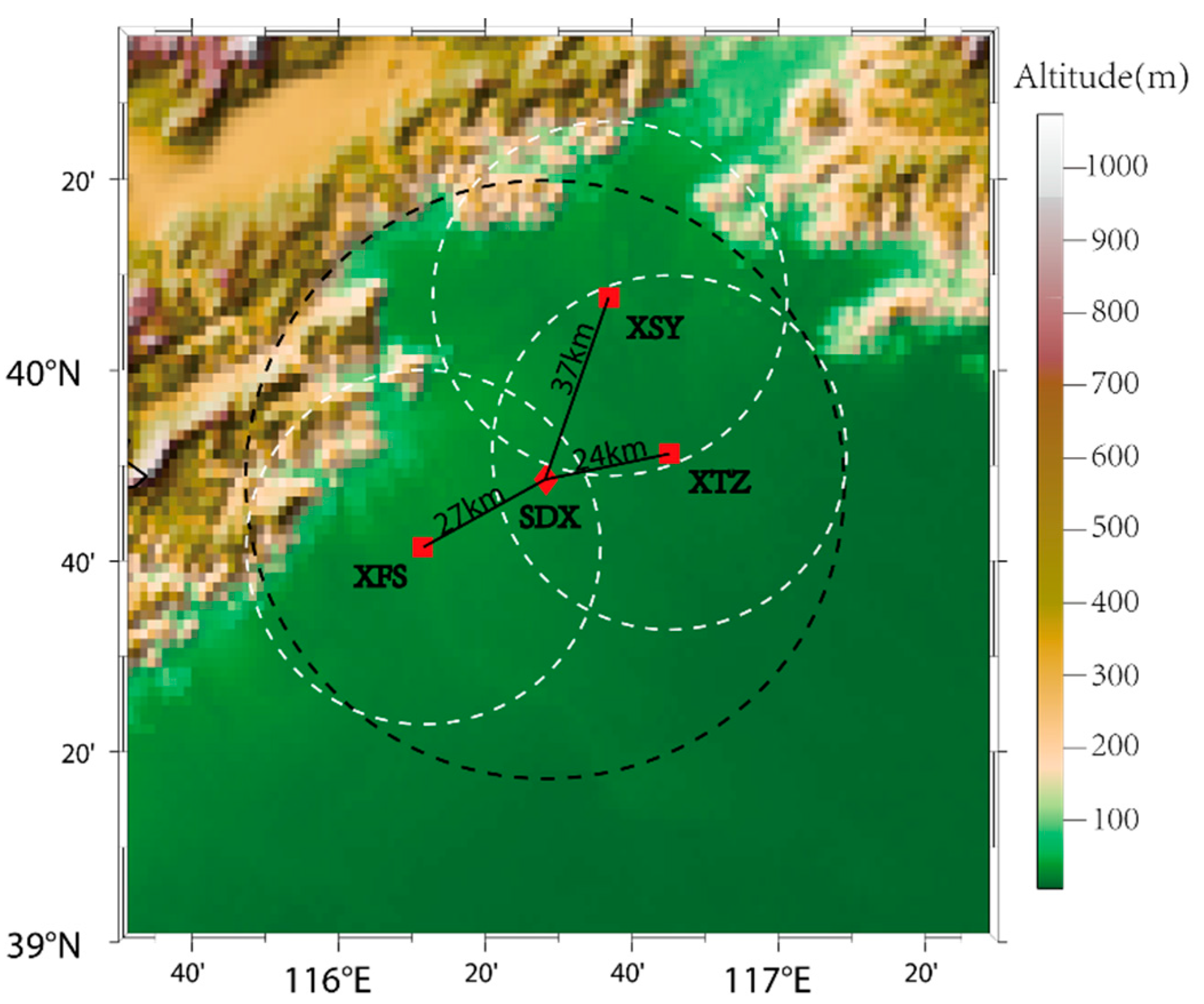
3.1. Instruments

The data of clear-air echoes used in this study were collected by China’s New Generation Weather Radar (CINRAD/SA radar) and three X-band dual-polarization (X-POL) radars with the same technical parameters [36]. CINRAD/SA was developed from the American WSR-88D (NEXRAD) through a joint agreement between the two countries [37]. The CINRAD/SA radar of Beijing is located in the Daxing district of Beijing and was fully upgraded with polarimetric capabilities in April 2021. The products of CINRAD/SA have a radial distance resolution of 250 m and an azimuthal resolution of 1 degree. The volume coverage pattern 21 (VCP21) scan mode was selected which sweeps 9 elevation angles of 0.5, 1.5, 2.4, 3.4, 4.3, 6.0, 9.9, 14.6, and 19.5 degrees in 6 min.

The X-POL radars were built by the Beijing Meteorologic Service to improve radar usage in weather monitoring. The stations of the X-POL radars used in this study are in the Fangshan, Shunyi, and Tongzhou districts of Beijing (the BJXFS, BJXSY, and BJXTZ sites, respectively), located around the CINRAD/SA radar sites. The positions of the four radars and terrain are shown in Figure 1. The scan strategy for the X-Pol radars is the same as the CINRAD/SA radar. The detailed system characteristics of the CINRAD/SA radar and the X-POL radars are shown in

Table 2. System characteristics of the CINRAD/SA radar and the X-POL radars.

Parameter	CINRAD/SA Radar	X-POL Radars
Frequency	2700–3000 MHz	9300–9500 MHz
Antenna cover diameter	11.9 m	≥4 m
Polarization	Linear H and V	Linear H and V
Volume coverage patterns	VCP 21	VCP 21
Time of VCP 21	6 min	3 min
Range resolution	250 m	75 m
Minimum detectable reflectivity	−7.5 dBZ @ 50 km	5 dBZ @ 60 km

.

The operations of all these radars are under the supervision of the CMA. The CINRAD/SA and the X-POLs are also calibrated weekly and monthly according to the technical standard of the CMA, which includes the system internal calibration, the receiving link calibration, the rotary joint calibration, and others.

Some meteorological parameters were used in this study. The profiles of the air temperature, the relative humidity, and the absolute humidity were collected using a microwave radiometer (RPG-HATPRO-G5, Meckenheim, Germany). The range resolution of the microwave radiometer was 50 m for heights below 1 km, 100 m for heights between 1 km and 2 km, and 250 m for heights from 2 km to 10 km, and the temporal resolution was 1 s. The wind vertical velocity and the wind shear were retrieved using a 3D Doppler wind lidar (Windcube 100 s, Leosphere, Saclay, France). The wind measurement products had a spatial resolution of 25 m with a temporal resolution of 20 s, and the products were not used when the carrier-to-noise ratio was less than −30 dB. A radar wind profiler (RWP) CFL-06, which was manufactured by the 23rd Institute of the China Aerospace Science and Industry Corporation, was also used to detect and process the profiles of the horizontal wind speed and direction. The radar wind profiler operates in the L-band (1290 MHz) and provides data with a vertical resolution of 120 m for heights between 150 m and 2.9 km. The microwave radiometer, the wind lidar, and the wind profile radar were located several tens of meters from the S-band weather radar in the same observation field.

3.2. Preprocessing

Preprocessing was needed before data comparison between multiple radars because of the differences temporally and spatially. It was necessary to preprocess and use multiple actual sounding data to create a time–height cross-section for the comparison about the DWR. The time–height cross-section is composed of vertical profiles of continuous time. Thus, the calculation of the vertical profile is introduced in the following sections.

3.2.1. Threshold

It is commonly believed that the signal of clear-air echoes is generally weak. A distorted signal would hamper the estimation of echoes. Hence, first, the signal-to-noise ratio (SNR) is set as the standard of thresholding. The minimum value of the SNR thresholding is 6 dB.

Secondly, the setting of the threshold needs to consider the limits of the radar’s minimum detectable reflectivity. If the echoes are out of the range of the radar system’s designed criteria, weak echoes may be distorted. The distortion values of the echoes then introduce errors into the statistics and the comparison. Meanwhile, the different minimums of the reflectivity values on different radar systems may affect the statistics as well. On the other hand, an excessive detection range would reduce the effectiveness of the comparison with the vertical observation system. Consequently, the radial distance from the radar to the objective is limited.

As shown in Table 2, the minimum detectable reflectivity of the CINRAD/SA and X-POLs was less than −7.5 dBZ at 50 km and 5 dBZ at 60 km. Therefore, balancing the minimum detectable reflectivity and the volume of the data, the range threshold of the data was 59 km for the S-band and 17 km for the X-band. The range threshold was set according to the radar equation to ensure that the radars with different wavelengths had the same minimum detectable reflectivity, which was −6 dBZ.

3.2.2. Vertical Profiles

The vertical profile of the reflectivity factor is useful to estimate the rainfall intensity because of the complexity of the vertical structure of radar echoes [38,39,40,41]. From radar data recorded at multiple elevation angles, the mean value of the reflectivity at each altitude can be calculated. Thus, the mean vertical profile of reflectivity (MVPR) can be easily extracted from volume-scan data. Unlike the MVPR, which focuses on the precision of the radar precipitation estimation, a method for determining the state of clear-air echoes needs to be presented.

For weak clear-air echoes, an extreme value can cause fluctuations in the mean value. The limited number of antenna elevation angles also introduces a discretization of the sampling of echoes and lessens the accuracy of the profile. Therefore, a minor alteration is being made to the MVPR.

Assuming the value of the reflectivity factor in a certain altitude range obeys the Gaussian distribution, the expected value of the reflectivity factor can be used to accurately estimate the state of the clear-air echoes at the sampling altitude. By applying Gauss curve fitting to the frequency distribution function of the reflectivity factor, the expected value can be obtained. The fitting uses the bi-square method for robustness, and the adjusted R-square of the effective fitting needs to be larger than 0.95.

Of special note is that a multiplicative adjustment factor is applied to the frequency distribution function because of the characteristics of the radar beam that make the volume of echoes different. The adjustment factor (called the weight factor) is the ratio of the single-sampling volume to the sum of the volume of the scan in the altitude range, or simply denoted by the sampling volume of the single echo.

It is also noticed that the fit coefficients are affected by the number of samples, so the sample size of the reflectivity factor needs to be checked at the sampling altitude. The minimum ratio of the sample size is set to 10%, which means the ratio of the valid sample to the total of the scan volume at the sampling altitude needs to be greater than one-tenth experientially in this study.

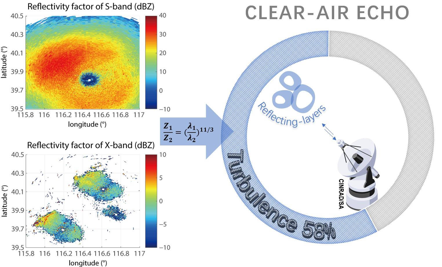
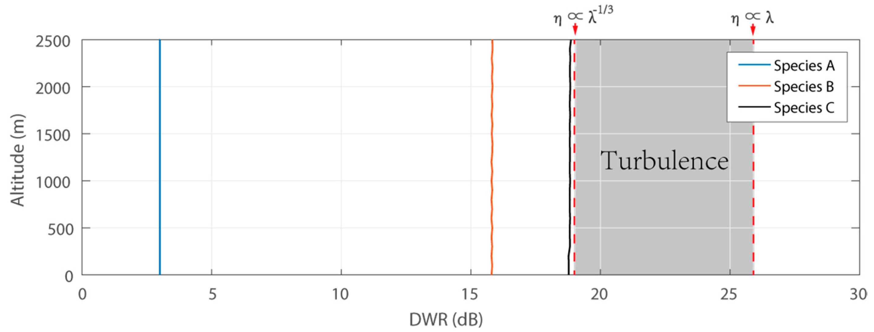
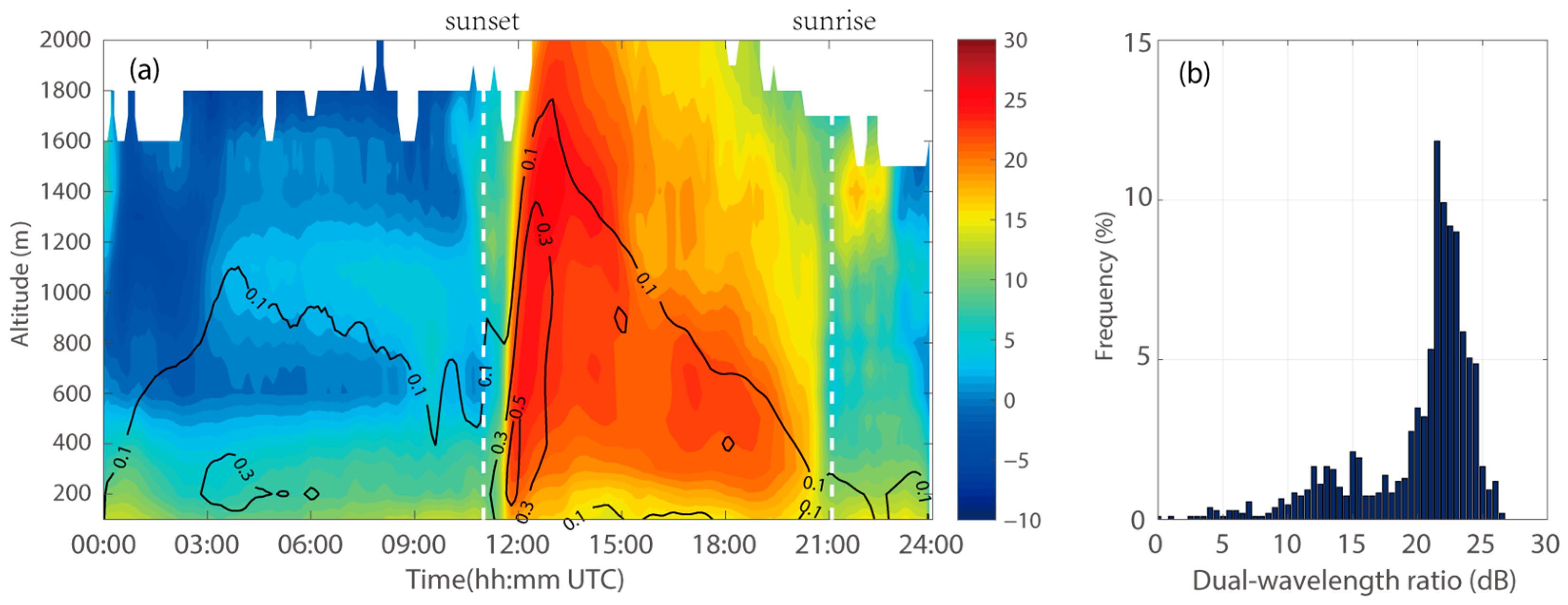
3.2.3. Dual-Wavelength Ratio

Unlike the differential reflectivity measured by means of two orthogonal signals that differ in polarization, the DWR describes the ratio of the radar reflectivity measured with two signals of different wavelengths. In Section 2, it has been found that biological scattering and turbulent scattering have different characteristics of the DWR. The DWR of Bragg scattering is dependent on the radar wavelength, as shown in Equation (9). Moreover, the DWR change in biological scattering is unpredictable because of the biologically complex shape. Hence, the predominant scattering mechanism can be determined by the DWR.

However, it is also known that the value of $Z$ from biological scatterers has an asymmetric pattern which depends on the angle between the radar beam and the main orientation of the biological scatterers. Moreover, values of the DWR may be more complicated and confusing because of the asymmetric pattern. Thus, it needs to examine the effect of the asymmetric pattern.

For the examination, the RCS of biological scatterers is simulated by the computer utilizing FEKO simulation software in this study [35]. The simulative value of RCS is dependent on many factors. One of the factors is the incident angle of the radar beam. Although biological scatterers appear randomly at each azimuth angle of the radar, the incident angle of the simulation is only decided by the angle between the incident beam and the biological scatterer. By changing the coordinate origin of the simulation from the location of the scatterer to the location of the radar, the incident angle can be converted to the azimuth angle when the directions of the biological scatterers are same.

Other parameters of the simulation are obtained from Table 1 based on the model of prolate spheroids of the spinal cord dielectric. Further, supposing that insects fly horizontally in the east–west direction and the density is one per cubic meter, the $Z$ value can be calculated by the simulated RCS shown in Figure 2. Figure 2 exemplifies the asymmetric pattern of the $Z$ values and is almost consistent with previous studies [42]. It is found that the asymmetric pattern may lead to confusion about the conclusions of Section 2.

However, the asymmetric pattern does not affect the results of the method in Section 3.2.3. The vertical profiles of the DWR between the S- and X-band are calculated and shown in Figure 3. The computation is deduced in terms of the scan mode of VCP21. Figure 3 shows that the vertical profiles of the DWR are same on each level of height, and the values are close to the simulation values of the insects’ body sizes. This is because the RCS of the insect size changes more slowly with angle. However, it is also found that the $Z$ difference values of large insects and the values of turbulence are close. Thus, the echo of turbulence is likely confused with that of large insects in the DWR.

Fortunately, large insects have a much stronger flight ability, and flight speed is correlated with body size in animals [43]. Research on the migratory behavior of armyworms expresses that the flight speed of armyworms during migration is greater than 4 m/s [44]. Thus, large insects can be easily distinguished by the velocity azimuth display (VAD). Analysis of the VAD is necessary to exclude confusion with large insects.

4. Results

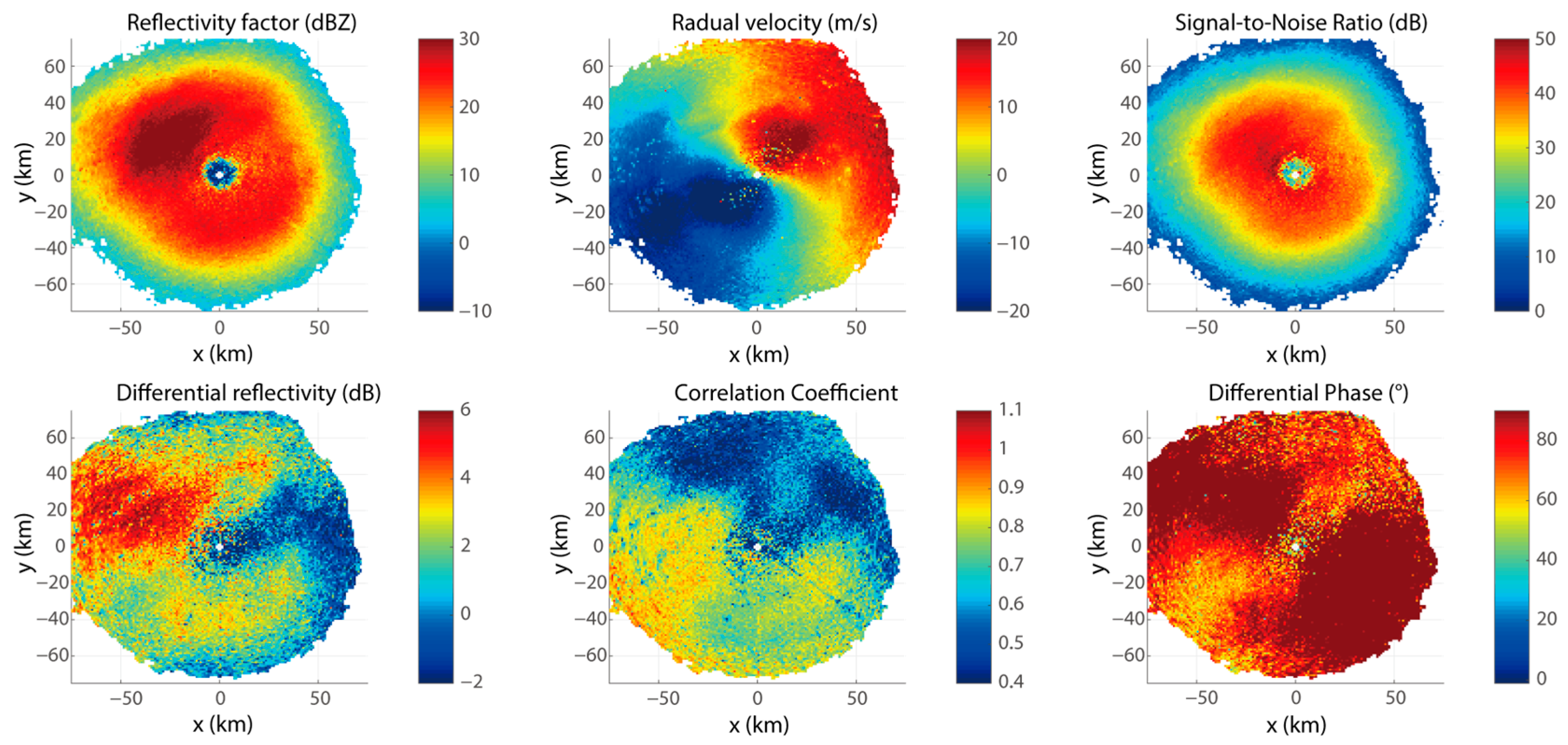
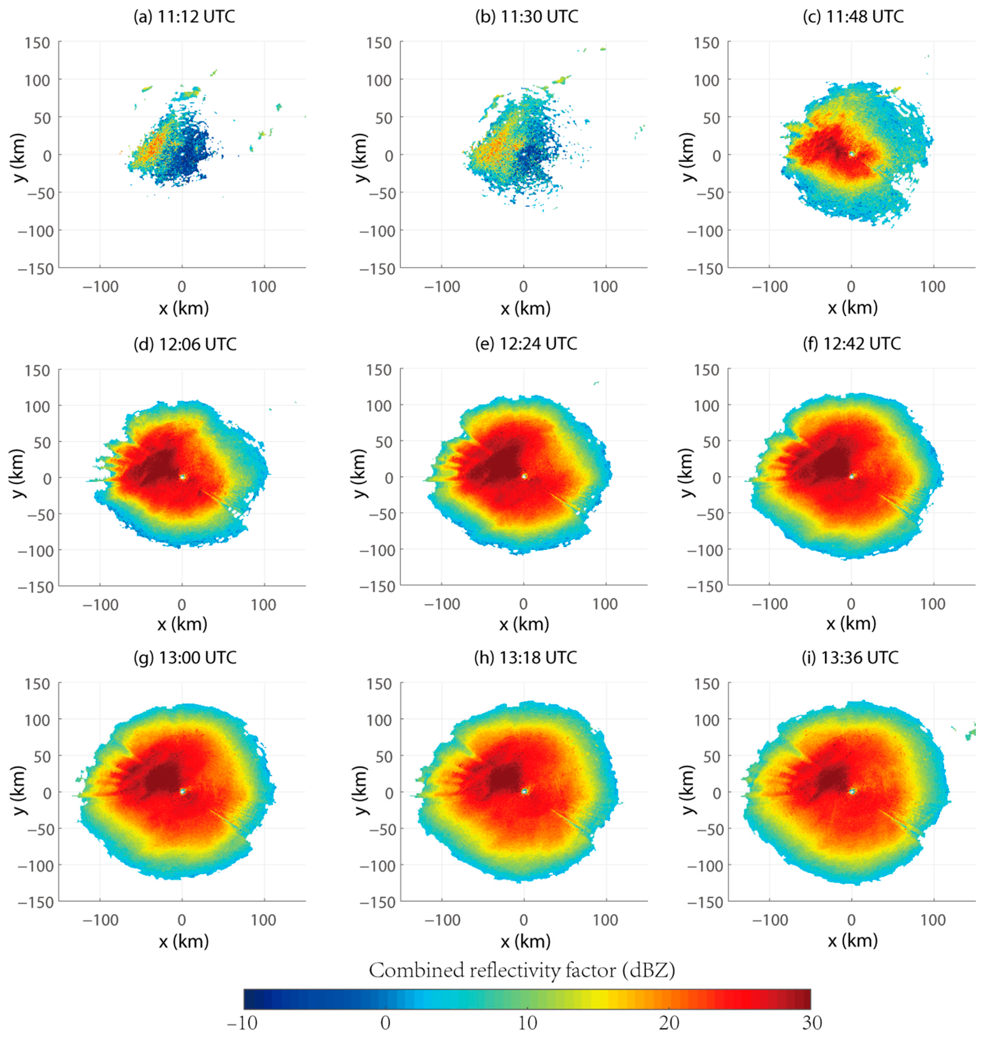
4.1. Plan Position Indicator

For the sake of discussion, the radar data from May 2 were taken as the case for further study. The focus of this case was from 11:30 (UTC), 2 May 2021, when the clear-air echo first appeared in the radar display, until it began to disappear at 20:30, when the echo became less distinct. The products in Figure 4 show that the echo was characterized by a low $Z$, a $Z_{DR}$ higher than that typically observed in meteorological echoes, and a correlation coefficient ${\rho }_{HV}$ lower than that observed in meteorological echoes. Generally, similar echoes have been observed in bird scattering comprising many species flying over Southern Kansas from Wichita, KS, USA [5].

Some researchers have indicated that the ${\rho }_{HV}$ varies with scatterer orientation, with birds flying away producing low ${\rho }_{HV}$ values and birds flying toward producing higher ${\rho }_{HV}$ values. However, the velocity–azimuth display (VAD) confirmed that there was no intense bird migration. Analysis of the VAD is used to determine spatially averaged kinematic properties of the velocity field. According to the function of the radar azimuth angle, the VAD of the wind field resembles a sine function. Moreover, during intense bird migrations, a huge difference in scattering of the observed radial velocity around the modeled radial velocities will be evident.

Figure 5 shows a high-quality wind VAD, which was the same passage of a cold front as observed by an operational weather radar in De Bilt [45], Netherlands. Only a small part of the residual error exhibited signs of bird activity. Since the nonzero value of the Doppler velocity due to bio-scatterers is representative of biological target movement, the temporal change in $Z$ is shown in Figure 6 to check for movement.

Figure 6 shows a continuous change in $Z$; the echoes began to increase rapidly at 11:30 and then remained basically unchanged after 12:06. It is strange that the echoes changed with the radar station as the center but not the “habitat”, and the echoes with a larger $Z$ also maintained their appearance. Whereas the value of the Doppler velocity was rhythmical, shown in Figure 7, the characteristics of the spatial distribution were also unchanged after 48 min, indicating that the scatterers did not move.

To confirm the state of the scatterers’ movement, in Figure 8, the range–height cross-section of $Z$ is displayed in the azimuth of the wind direction. As shown in Figure 8, the signal was enhanced along the height at each range and did not change following wind direction. The phenomena discovered by Adriaan were not observed [46]. Paradoxically, the scatterer remained in the air, but the Doppler velocity was a nonzero value.

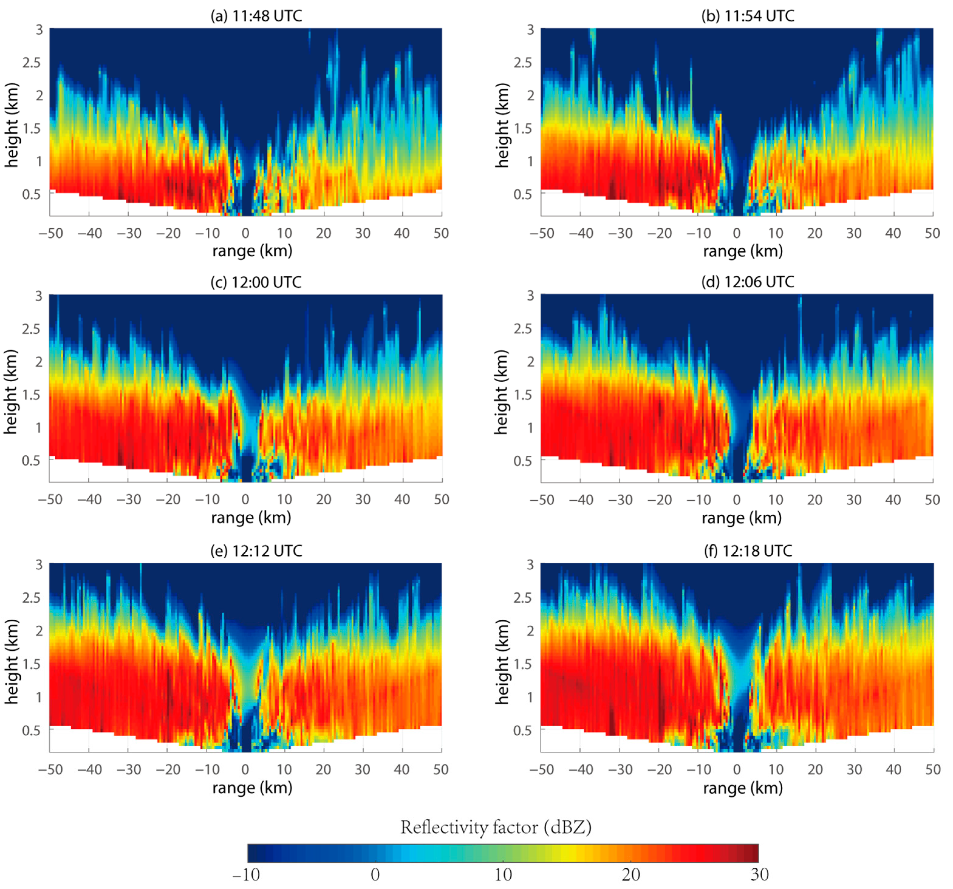
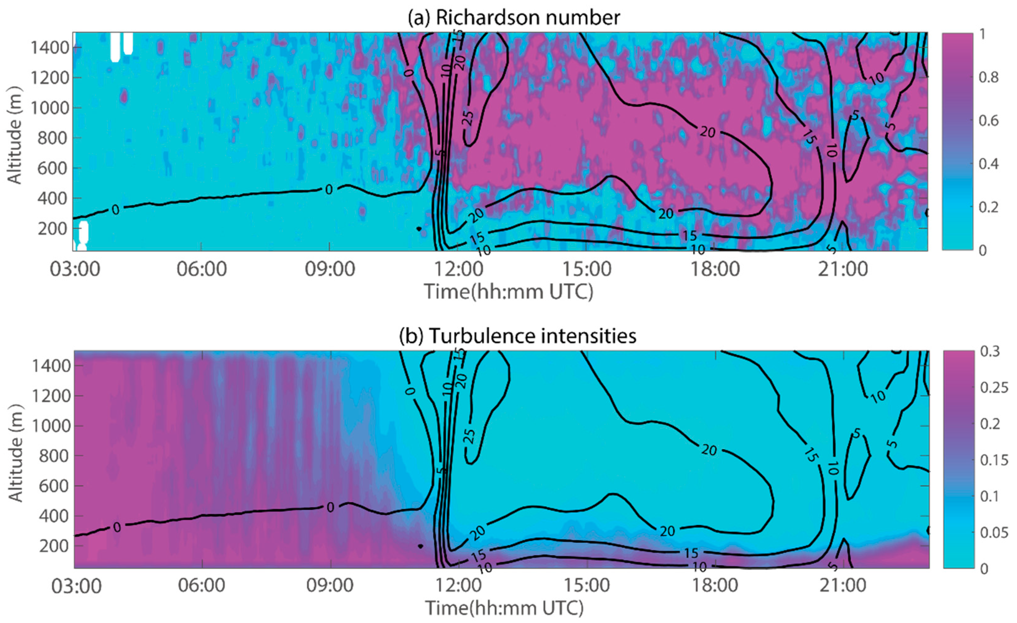
4.2. Time–Height Cross-Section

Movement is the most important feature of bio-scatterers. To reveal the causes of clear-air echoes, the radar data were displayed as a time–height cross-section. The signal of the clear-air echoes showed significant diurnal variations, as shown in Figure 9. It was thought that the activities of nocturnal creatures caused greater echoes. However, the rapid growth in the signal in the time–height cross-section caught our attention. Surprisingly, the value of $Z$ grew fast. The 23 dBZ echo only took 13 min to increase from 500 m to 1000 m, and the increasing velocity was 0.64 m/s. When using the wind lidar, as Figure 10 shows, the vertical velocity of the wind was below 0.5 m/s and was smaller than the velocity of the echoes. This indicates that a small bio-scatterer, which does not fly well, could not be the scatterer. Despite the impractical state of motion, perhaps these clear-air echoes were still caused by large bio-scatterers. However, the vertical profiles of $Z_{DR}$ shown in Figure 9 deny this view.

It is known that $Z_{DR}$ is the radar reflectivity difference between the horizontal and vertical polarization and represents the dimension of the scatterer. If the measurements of the volumes contain multiple scatterers, $Z_{DR}$ will be biased toward the characteristics of the largest scatterers. In Figure 9, the profiles of $Z_{DR}$ increased with height and were temporarily greater than 2.5 dB above an altitude of 1200 m. Scatterers with a 2.5 dB $Z_{DR}$ do not climb from the ground and do not land. This implies that the echoes did not float from the ground into the air, but they suddenly appeared in the middle of the air without immigration.

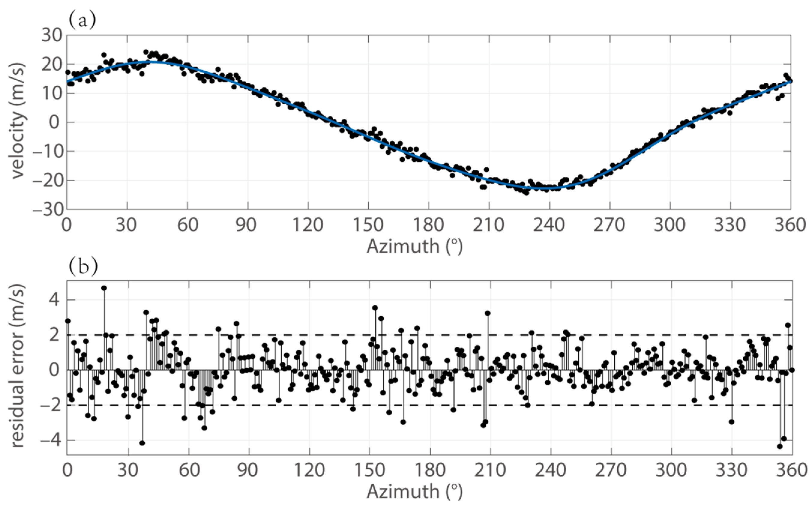
4.3. Velocity Analysis

Although we have preliminarily analyzed the VAD in Section 4.1, to avoid confusion with large insects and birds, the Doppler velocity and the results of the VAD analysis are displayed in Figure 11 again. In Figure 11, the velocity fields, which were obtained from the VAD analysis, are similar to the radar Doppler velocity. The residual values of the velocity fields are shown in Figure 12a. in total, 86.4% of the residual values are less than 4 m/s, and 65.3% of the values are less than 2 m/s. The echoes were unlikely caused by large insects and birds mainly because large insects and birds have quite a great flight speed and would make the speed field messy and produce great deviations.

The comparison of the speed profiles with the RWP and the CINRAD/SA confirms the conclusion. The profiles of the horizontal wind speed which were sensed by the RWP are not different from the speed profiles calculated by the CINRAD/SA, as shown in Figure 12b. Despite the system deviation in Figure 12b, which is common in the results of the VAD wind profile [47], the changes in the speed profiles are consistent, generally. The profiles of the CINRAD/SA indicate that clear-air echoes are moving with the wind speed. However, the speed of biological autonomous movement is not detected by the weather radar. This means that these echoes are unlikely to be caused by creatures with a strong flight ability such as birds and large insects.

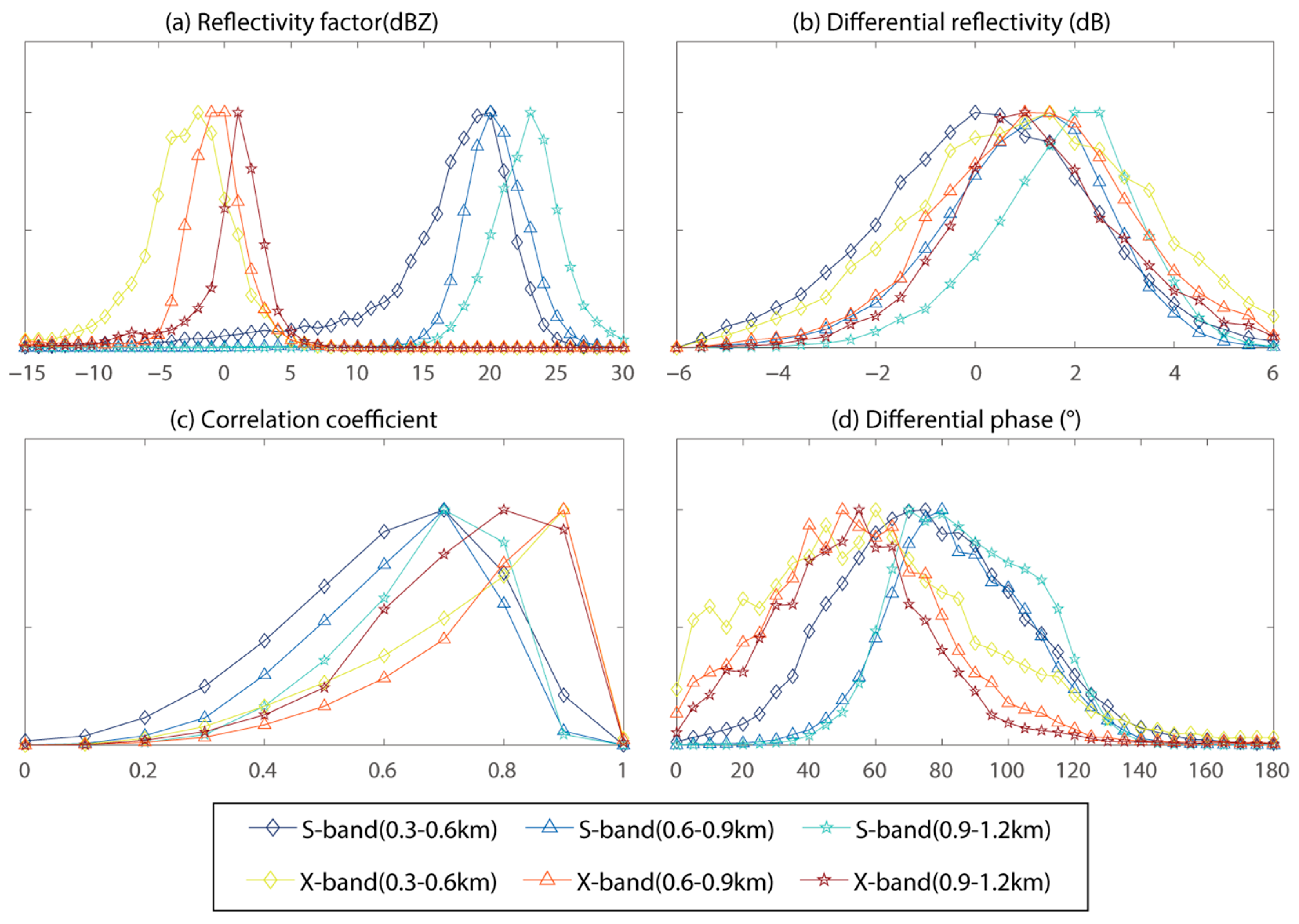
4.4. Comparison of the S-Band and X-Band

In Section 4.1 and Section 4.2, some contradictions of bio-scatterers were revealed, and a quantitative analysis of the echoes was thus needed to convincingly demonstrate the cause of the clear-air echoes. A comparison of the reflectivity factors of the two bands is another method that can be used to determine the cause of clear-air echoes. Since the DWR of the turbulence echoes in different bands was more regular than biological, the time–height cross-section of $Z$ using the data from BJXFS is shown in Figure 13, and the DWR between the S-band and the X-band is displayed in Figure 14.

In Figure 13, intuitively, the signal of the X-band differed from the S-band signal in the value of $Z$; the value of the X-band was much smaller than that of the S-band. The signal of the X-band also did not have an as pronounced diurnal variation as that of the S-band echoes. Although the signal of the X-band echoes appeared as fast as those of the S-band signal at dusk, the signal did not last long and slowly vanished from the top to the bottom after 13:00. Meanwhile, the value of $Z$ in Figure 13 is low at lower altitudes and increases with height, which is different in Figure 9. This is due to the minimum scale of turbulence which increases with height. When the minimum scale exceeds the half-wavelength of the X-band, which is still much smaller than the wavelength of the S-band, the scattering vanishes before the refractivity gradient weakens. Hence, the $Z$ value of the X-band seems to increase progressively without reducing.

Figure 14a shows the time–height cross-section of the DWR between the $Z$ values of the CINRAD/SA and X-POLs, and Figure 14b shows the normalized frequency histograms for the radar fields in Figure 14a. The histogram of the DWR shows the characteristic values near 21.5 dB. Moreover, the $Z$ value distributions of the S-band and X-band also show that the peaks of the $Z$ values are at intervals of about 22 dB (in Figure 15), whereas the $Z_{DR}$ distribution does not peak at 0 dB. In Figure 15, the frequency distribution of the $Z$ value resembles the Gaussian distribution and slightly changes with height, which is in line with the condition of the hypothesis in Section 3.2. However, it is not expected that the correlation or other products should follow the Gaussian distribution. The distributions of turbulence variables deviate from normality because of the intermittence [48,49,50].

The large widths of these distributions match with the characteristics of bird echoes seemingly. However, the echo is unlikely to be mainly caused by birds for the following reasons. First, the analysis of the VAD has already denied the dominance of birds. Second, for north China, May is almost the end of the spring migration and is close to the period of preincubation, yet the scatterers of the clear-air echo still travel to the north until late July [51,52]. Third, there are two international airports located at the azimuth angles of 22° and 188° and the distances of 31 km and 34 km, respectively. The large numbers of birds migrating would obviously be a threat to the safety of the flights if the clear-air echo was caused by birds. Therefore, the suspicion of birds and large insects has been ruled out.

It is worth noting that the CINRAD/SA and X-POL are located along the same migration path. It means that the two radars should observe the same group of scatterers with the same scattering characteristic, moving from upstream (XFS) to downstream (SDX) the whole night, continuously. Although Z values from atmospheric insects may have asymmetric patterns which depend on the angle between the radar beam and the main orientation of the biological scatterers, the time–height cross-section of the Z values will not be affected because the cross-sections are counted by the whole coverage volume of the radar observation and are not dependent on the azimuth. Thus, the asymmetric patterns cannot stain the ratio between the Z values of the CINRAD/SA and X-POL.

It is already known that, according to Equation (6) and Equation (10), the $Z$ difference in the turbulence of the S-band (2870 MHz, 10.45 cm) and the X-band (9455 MHz, 3.17 cm) is about 19.0 dB and 21.4 dB, respectively. Since many creatures are within the size threshold for Mie scattering and have different RCSs at different wavelengths, the reflectivity relationships to the wavelength are far from straightforward. Meanwhile, wide discrepancies are found between the characteristics of clear-air echoes and the law of biological activities. Therefore, this proves that the Beijing CINRAD/SA echoes are mainly caused by turbulence.

The DWR statistics for the region of Beijing reveal that, from 1 May 2021 to 20 May 2021, 58% of the DWR was distributed between 18dB and 24dB, which is the characteristic interval of turbulence. Moreover, the clear-air echoes maintain the features of the variations in the $Z$ values and the VAD analysis. It means that nearly 58% of the echoes were probably caused by turbulence and proves that the influence of turbulence is erroneously ignored in clear-air echoes. Almost all these echoes did not show the classic features of Bragg scattering, such as a low $Z$ and zero $Z_{DR}$. These echoes could wrongly be identified as bio-scatterers and cause a misestimation of biomass. The number of flying creatures observed by the weather radar was much smaller than previously thought.

5. Discussion

Many scholars deny or reject the domination of turbulence in clear-air echoes. First, they propose that a nonzero $Z_{DR}$ indicates that the scattering is due to creatures rather than turbulence because, according to the statement of Kolmogorov’s theory that turbulence is homogeneous and isotropic, the $Z_{DR}$ of turbulent echoes should be zero. However, a problem with this viewpoint is that non-Kolmogorov turbulence widely exists in the atmospheric boundary layer. Some observations have already shown that the atmospheric structure constant of the refractive index differs between the horizontal direction and the vertical direction. Therefore, the $Z_{DR}$ cannot support their rejections. We agree that biological scatterers cause large values of $Z_{DR}$, but the contribution from the effect of turbulence still needs to be investigated.

Second, some scholars believe that because the $C_n^2$ calculated from echoes is larger than the high end of the observed values, clear-air echoes should not be attributed to turbulence. For example, clear-air echoes of a 10 to 20 dB $Z$ require $C_n^2$ to be greater than ${10}^{-11} m^{-2/3}$, which is far above the observed $C_n^2$. The phenomenon of clear-air echoes cannot be explained by Bragg scattering. Therefore, it is assumed that the domination of clear-air echoes is not turbulence. However, scholars have ignored the effect of another scattering mechanism. We found another reasonable scattering mechanism to explain clear-air echoes in communication and wireless areas.

In communication, tropospheric scattering (also known as troposcatter) is admitted as an efficient propagation method by the Radiocommunication Sector of the International Telecommunication Union, which describes the mechanism by which microwave radio systems inadvertently achieve beyond-the-horizon communications [53]. One of the three models of the troposcatter is the reflecting-layers model. The other two models are scattering from turbulence and reflections from an exponential atmosphere. Tropospheric scattering is the result of the combination of these three models. Zhang points out that the reflectivity of the troposcatter can be written as follows [54]:

$$\eta =B\overline{{\left(\frac{\mathrm{d}{\epsilon }_r}{\mathrm{d}h}\right)}^2}{\lambda }^n{\left(2\phi \right)}^{-m}$$

(11)

where $B$, $n$, and $m$ are constants and are measured by experiments; ${\epsilon }_r$ is the dielectric constant; $h$ is the height; $\phi$ is the glancing angle; the bar is the sign of the mean; and the relationship between ${\epsilon }_r$ and $h$ can refer to the assumption by K. Bullington [55]. Interestingly, the scattering from turbulence is essentially the same as Bragg scattering, but few studies have highlighted the role of reflecting layers in clear-air echoes.

To demonstrate how reflecting layers affect clear-air echoes, we calculated the gradient Richardson number and the intensity of the turbulence (expressed by the ratio of the standard deviation of the wind speed to the mean wind speed) using a microwave radiometer and a wind lidar [56,57]. Moreover, the atmospheric profiles were collected by a microwave radiometer. Although the geometrical structure of the reflecting layers remains obscure, it can be inferred that turbulent mixing is detrimental to the reflecting layers because a reflecting layer in the atmosphere is formed by relatively sharp gradients of the refractive index, but turbulent mixing makes the temperature and humidity homogeneous and reduces the gradient of the refractive index. Thus, the Richardson number and the turbulence intensity, which indicate turbulent mixing, are shown in Figure 16 to give the relationship between clear-air echoes and turbulent mixing.

In Figure 16, large values of $Z$ correspond to large Richardson numbers and turbulent mixing. When the sun sets in the west, the turbulent mixing rapidly weakens. Additionally, the unmixed air masses with relatively sharp gradients become the reflecting layer and generate the scattering signal of the clear-air echoes. In contrast, in the daytime, the strong turbulent mixing breaks the structure of the reflecting layer, and only the turbulent scattering remains. Thus, turbulence has a greater impact on the echoes at night than in the daytime.

The same diurnal variation has been observed in the field-strength variation in the short radio wave propagation in Arizona [58]. Other studies have found that troposcatter propagation only occurs when the turbulence scale is larger than the wavelength of the radio signal, and the signal level with a wavelength of 9 cm is much larger than that with a wavelength of 3 cm [58,59]. These phenomena have the same characteristics as clear-air echoes, with the value of the reflectivity factor at the S-band being bigger than that at the X-band. Thus, we propose that the reflecting layers cause a diurnal variation in clear-air echoes and enhance the signal of clear-air echoes at night. Therefore, the coexistence of the reflecting layers and Bragg scattering is the reason why the value of $C_n^2$ calculated from the echoes is larger than the value from the theoretical calculations. Further, the reflecting layers explain some of the characteristics of $Z_{DR}$. For example, the vertical signal of clear-air echoes is weaker than the horizontal signal because turbulent mixing is stronger in the vertical direction, and the vertical reflecting layers cannot easily survive. Thus, the values of $Z_{DR}$ are generally greater than zero.

An interesting note is that the high reflectivity area in the upper-left region of Figure 4 analyzes the characteristics of a low correlation coefficient, and in this area, $Z_{DR}$ presents a mixture of high and low values. This characteristic is ascribed to the atmospheric response to the underlying surface, which belongs to a mountainous region and is quite different from the others in Figure 1.

The rough terrain of mountains makes the turbulence more chaotic and intense, which produces a stronger refractive index and scattering. A thin layer of shear turbulence excited on the shear plane makes the $Z_{DR}$ larger, but the layer is not stable, bringing a mixture of high and low values to the $Z_{DR}$. However, it is noted that, by upthrust, too high mountains may affect the turbulent scales, which are too large to match up to the radar wavelength for scattering. The relationship between the underlying surface and clear-air echoes is worth further exploration in the future.

Another interesting characteristic of the $Z_{DR}$ is that its value grows weak and becomes close to zero in the day–night shift scenes. We speculate that the turbulent mixing reaches a quasi-equilibrium state, and this will be further investigated in future studies.

Yet despite all this, some scholars still express a slightly different point of view. They claim that the reflection from turbulent air at the S-band has been studied by some studies [29,60,61,62,63], and it has been well established with polarization radars that turbulent air has $Z_{DR}$ values close to 0 dB at the S-band. However, these echoes were commonly observed at the top of the convective boundary layer (also called the entrainment layer). The entrainment layer is essentially static in stability. Due to the effects of penetrative convection and entrainment, thermals reciprocate in the layer [64]. The reciprocation brings turbulence generation on the one hand; on the other hand, the stable air brings the turbulence closer to a locally homogeneous isotropic state. Thus, the observed echoes can be regarded as special cases and cannot represent the whole characteristic of clear-air turbulent echoes. Figure 17 shows the vertical profiles of the $Z$ values and rawinsonde data. It is observed that there is a layer of enhanced reflectivity at the entrainment layer, which is consistent with the known results [63].

Some scholars also conject that dust and other particulate matter can be the cause of the clear-air echoes. At the beginning of this study, we also inferred that nocturnal pollutant accumulation is the reason for the echo diurnal variation because of the uncleanliness of the atmosphere of the megacities. Yet, it is hard to explain the variation in the echo signal.

One piece of evidence is based on seasonal variation. In winter, the air quality is the worst because of heating, which uses fossil fuels, but the clear-air echo is hardly observed by radars during winter. The annual and monthly variation in the sand and dust also showed that the sand and dust weather is most frequent in spring, whereas the signal of the spring clear-air echo was generally weaker than summer and autumn.

The other piece of evidence comes from the daily change in pollutants. The concentration of pollutants has two peaks because of traffic congestion in the metropolis, which is different from the $Z$ value. The wind, which is related to pollutant diffusion and dust, also does not show a significant correlation with the clear-air echoes. Although it is known that fire plumes can cause clear-air echoes [65,66], it is unrealistic to detect plumes of wild fires in an urban area. Thus, dust and the pollutants are unlikely to be the main causes of clear-air echoes.

The issue of the influence of meteorological factors on troposcatter communication remains unknown and requires future examination. In troposcatter, the value of the signal level depends on the refractive index and its gradient, which are affected by the intensity of the turbulence fluctuation and atmospheric stratification. Thus, Gaoming Zhang proposed that the inversion of temperature leads to the diurnal variation in the signal [54]. However, few studies focus on the effect of turbulent mixing on signals level. Thus, we plan to provide a more in-depth explanation of reflecting layers forming and the structure of the nocturnal boundary layer in future studies. Meanwhile, Guifu Zhang pointed that bistatic radars have an advantage in the sensitivity of clear echoes [67]. Technically, experiments using bistatic radars are closer to the principle of troposcatter propagation. Moreover, experiments with bistatic radar data would provide more information for the analysis in future research.

6. Conclusions

In this study, clear-air echoes detected by CINRAD were analyzed to find their causes. Some observations diverge from the previous conclusion that bio-scatterers are the main reason for clear-air echoes.

Echoes with a larger Z are not deformed in the air, even if the scatterers are moving. The change in echoes in the vertical direction is also closer to the switching of the physical mode rather than biological flying. The analysis results of the DWR and the VAD support that turbulence plays an important role in clear-air echoes. In the case of May 2, the frequency distribution of the DWR peaks at 21.5 dB, which is consistent with the theory of turbulence. From 1 May to 20 May, 58% of the DWR between the S-band and the X-band is distributed between 18 dB and 24 dB, which means that more than half of the echoes at night were caused by turbulence. It was confirmed that the influence of turbulence is erroneously ignored in clear-air echoes. The reflecting-layers model of troposcatter propagation is the cause of the clear-air echoes, and this model can explain the main phenomena of the radar observations.

This study provides initial evidence for a case study in Beijing that the model based on Kolmogorov’s theory may not be tenable for all clear-air echoes, highlighting the need for an expanded set of causes of clear-air echoes. The reflecting-layers model, which is one of the three models of tropospheric scattering, cause a diurnal variation in clear-air echoes and enhances the signal of clear-air echoes at night. Unmixed air masses with relatively sharp gradients become the reflecting layer and generate the scattering signal of clear-air echoes.

With the help of the theory of troposcatter propagation, rapid progress will be made in the ecological monitoring method of weather radars. A more objective and comprehensive study of clear-air echoes can effectively make weather radars acceptable in biological research instead of ignoring irrationalities. With the help of weather radars, ecology will be able to develop strongly and continuously in the near future.

References

1. Van Doren, B.M.; Horton, K.G. A continental system for forecasting bird migration. Science 2018, 361, 1115–1117. [Google Scholar] [CrossRef] [PubMed]
2. Bruderer, B. The study of bird migration by radar part 1: The technical basis. Naturwissenschaften 1997, 84, 1–8. [Google Scholar] [CrossRef]
3. Wilson, J.W.; Weckwerth, T.M.; Vivekanandan, J.; Wakimoto, R.M.; Russell, R.W. Boundary Layer Clear-Air Radar Echoes: Origin of Echoes and Accuracy of Derived Winds. J. Atmos. Ocean. Technol. 1994, 11, 1184–1206. [Google Scholar] [CrossRef]
4. Martin, W.J.; Shapiro, A. Discrimination of bird and insect radar echoes in clear air using high-resolution radars. J. Atmos. Ocean. Technol. 2007, 24, 1215–1230. [Google Scholar] [CrossRef]
5. Van den Broeke, M.S. Polarimetric Radar Observations of Biological Scatterers in Hurricanes Irene (2011) and Sandy (2012). J. Atmos. Ocean. Technol. 2013, 30, 2754–2767. [Google Scholar] [CrossRef] [Green Version]
6. Westbrook, J.K.; Eyster, R.S.; Wolf, W.W. WSR-88D doppler radar detection of corn earworm moth migration. Int. J. Biometeorol. 2014, 58, 931–940. [Google Scholar] [CrossRef] [PubMed]
7. Zrnic, D.S.; Ryzhkov, A.V. Observations of insects and birds with a polarimetric radar. IEEE Trans. Geosci. Remote Sens. 1998, 36, 661–668. [Google Scholar] [CrossRef]
8. Ottersten, H. Atmospheric Structure and Radar Backscattering in Clear Air. Radio Sci. 1969, 4, 1179–1193. [Google Scholar] [CrossRef]
9. Kolmogorov, A.N.; Levin, V.; Hunt, J.C.R.; Phillips, O.M.; Williams, D. The local structure of turbulence in incompressible viscous fluid for very large Reynolds numbers. Rep. AS USSR 1941, 434, 9–13. [Google Scholar] [CrossRef]
10. Kolmogorov, A.N. A refinement of previous hypotheses concerning the local structure of turbulence in a viscous incompressible fluid at high Reynolds number. J. Fluid Mech. 1962, 13, 82–85. [Google Scholar] [CrossRef] [Green Version]
11. Mandelbrot, B.B. Intermittent turbulence and fractal dimension: Kurtosis and the spectral exponent 5/3 + B. In Multifractals and 1/ƒ Noise: Wild Self-Affinity in Physics (1963–1976); Mandelbrot, B.B., Ed.; Springer: New York, NY, USA, 1976; pp. 389–415. [Google Scholar]
12. Ringuet, E.; Rozé, C.; Gouesbet, G. Experimental observation of type-II intermittency in a hydrodynamic system. Phys. Rev. E 1993, 47, 1405–1407. [Google Scholar] [CrossRef] [PubMed]
13. Batchelor, G.K.; Townsend, A.A.; Jeffreys, H. The nature of turbulent motion at large wave-numbers. Proc. R. Soc. Lond. Ser. A Math. Phys. Sci. 1949, 199, 238–255. [Google Scholar] [CrossRef]
14. Pomeau, Y.; Manneville, P. Intermittent transition to turbulence in dissipative dynamical systems. Commun. Math. Phys. 1980, 74, 189–197. [Google Scholar] [CrossRef]
15. Siggia, E.D. Numerical study of small-scale intermittency in three-dimensional turbulence. J. Fluid Mech. 1981, 107, 375–406. [Google Scholar] [CrossRef] [Green Version]
16. Paladin, G.; Vulpiani, A. Anomalous scaling laws in multifractal objects. Phys. Rep. 1987, 156, 147–225. [Google Scholar] [CrossRef]
17. Huang, Y.N.; Huang, Y.D. On the transition to turbulence in pipe flow. Phys. D Nonlinear Phenom. 1989, 37, 153–159. [Google Scholar] [CrossRef]
18. Meneveau, C.; Sreenivasan, K.R. Interface dimension in intermittent turbulence. Phys. Rev. A 1990, 41, 2246–2248. [Google Scholar] [CrossRef]
19. Vassilicos, J.C. Turbulence and intermittency. Nature 1995, 374, 408–409. [Google Scholar] [CrossRef]
20. Benzi, R.; Biferale, L. Intermittency in Turbulence. In Theories of Turbulence; Oberlack, M., Busse, F.H., Eds.; Springer: Vienna, Austria, 2002; pp. 1–76. [Google Scholar]
21. Jiménez, J. Intermittency in Turbulence. In Encyclopedia of Mathematical Physics; Françoise, J.-P., Naber, G.L., Tsun, T.S., Eds.; Academic Press: Oxford, UK, 2006; pp. 144–151. [Google Scholar]
22. Belen’kii, M.S. Effect of the stratosphere on star image motion. Opt. Lett. 1995, 20, 1359–1361. [Google Scholar] [CrossRef]
23. Korotkova, O.; Toselli, I. Non-Classic Atmospheric Optical Turbulence: Review. Appl. Sci. 2021, 11, 8487. [Google Scholar] [CrossRef]
24. Rao, C.; Jiang, W.; Ling, N. Spatial and temporal characterization of phase fluctuations in non-Kolmogorov atmospheric turbulence. J. Mod. Opt. 2000, 47, 1111–1126. [Google Scholar] [CrossRef]
25. Andrews, L.C. Free-space optical system performance for laser beam propagation through non-Kolmogorov turbulence. Opt. Eng. 2008, 47, 026003. [Google Scholar] [CrossRef] [Green Version]
26. Li, Y.; Zhu, W.; Wu, X.; Rao, R. Equivalent refractive-index structure constant of non-Kolmogorov turbulence. Opt. Express 2015, 23, 23004–23012. [Google Scholar] [CrossRef]
27. Ruizhong, R.; Yujie, L. Light Propagation through Non-Kolmogorov-Type Atmospheric Turbulence and Its Effects on Optical Engineering. Acta Opt. Sin. 2015, 35, 0501003. [Google Scholar] [CrossRef]
28. Yang, H.; Fang, Z.; Li, C.; Deng, X.; Xing, K.; Xie, C. Atmospheric Optical Turbulence Profile Measurement and Model Improvement over Arid and Semi-arid regions. Atmos. Meas. Tech. Discuss. 2021, 2021, 1–14. [Google Scholar] [CrossRef]
29. Richardson, L.M.; Cunningham, J.G.; Zittel, W.D.; Lee, R.R.; Ice, R.L.; Melnikov, V.M.; Hoban, N.P.; Gebauer, J.G. Bragg Scatter Detection by the WSR-88D. Part I: Algorithm Development. J. Atmos. Ocean. Technol. 2017, 34, 465–478. [Google Scholar] [CrossRef]
30. Villars, F.; Weisskopf, V.F. The scattering of electromagnetic waves by turbulent atmospheric fluctuations. Phys. Rev. 1954, 94, 232–240. [Google Scholar] [CrossRef]
31. Stepanian, P.M.; Horton, K.G.; Melnikov, V.M.; Zrnic, D.S.; Gauthreaux, S.A. Dual-polarization radar products for biological applications. Ecosphere 2016, 7, 27. [Google Scholar] [CrossRef]
32. Park, H.S.; Ryzhkov, A.V.; Zrnić, D.S.; Kim, K.-E. The Hydrometeor Classification Algorithm for the Polarimetric WSR-88D: Description and Application to an MCS. Weather Forecast. 2009, 24, 730–748. [Google Scholar] [CrossRef] [Green Version]
33. Kilambi, A.; Fabry, F.; Meunier, V. A Simple and Effective Method for Separating Meteorological from Nonmeteorological Targets Using Dual-Polarization Data. J. Atmos. Ocean. Technol. 2018, 35, 1415–1424. [Google Scholar] [CrossRef]
34. Koistinen, J. Bird migration patterns on weather radars. Phys. Chem. Earth Pt B-Hydrol. Ocean. Atmos. 2000, 25, 1185–1193. [Google Scholar] [CrossRef]
35. Hu, C.; Fang, L.; Wang, R.; Zhou, C.; Li, W.; Zhang, F.; Lang, T.; Long, T. Analysis of Insect RCS Characteristics. J. Electron. Inf. Technol. 2020, 42, 140–153. [Google Scholar]
36. Wang, C.; Wu, C.; Liu, L.; Liu, X.; Chen, C. Integrated Correction Algorithm for X Band Dual-Polarization Radar Reflectivity Based on CINRAD/SA Radar. Atmosphere 2020, 11, 119. [Google Scholar] [CrossRef] [Green Version]
37. Chen, Y.; Zou, Q.; Han, J.; Cluckie, I. Cinrad data quality control and precipitation estimation. Proc. Inst. Civ. Eng.—Water Manag. 2009, 162, 95–105. [Google Scholar] [CrossRef]
38. Vignal, B.; Andrieu, H.; Creutin, J.D. Identification of Vertical Profiles of Reflectivity from Volume Scan Radar Data. J. Appl. Meteorol. 1999, 38, 1214–1228. [Google Scholar] [CrossRef]
39. Joss, J.; Lee, R. The Application of Radar Gauge Comparisons to Operational Precipitation Profile Corrections. J. Appl. Meteorol. 1995, 34, 2612–2630. [Google Scholar] [CrossRef]
40. Joss, J.; Waldvogel, A.; Collier, C.G. Precipitation Measurement and Hydrology. In Radar in Meteorology: Battan Memorial and 40th Anniversary Radar Meteorology Conference; Atlas, D., Ed.; American Meteorological Society: Boston, MA, USA, 1990; pp. 577–606. [Google Scholar]
41. Cuihong, W.; Yufa, W.; Tao, W.; Hongxiang, J. Vertical Profile of Radar Echo and Its Deteermination Methods. J. Appl. Meteorol. Sci. 2006, 17, 232–239. [Google Scholar]
42. Melnikov, V.M.; Istok, M.J.; Westbrook, J.K. Asymmetric Radar Echo Patterns from Insects. J. Atmos. Ocean. Technol. 2015, 32, 659–674. [Google Scholar] [CrossRef]
43. Farisenkov, S.E.; Kolomenskiy, D.; Petrov, P.N.; Engels, T.; Lapina, N.A.; Lehmann, F.O.; Onishi, R.; Liu, H.; Polilov, A.A. Novel flight style and light wings boost flight performance of tiny beetles. Nature 2022, 602, 96–100. [Google Scholar] [CrossRef]
44. Xingfu, J. The Physiological and Genetic Characteristics of Migratory Behavior and Genetic Diversity, as Determined by AFLP in the Oriental Armyworm, Mythimna Separata (Walker). Ph.D. Thesis, Chinese Academy of Agricultural Sciences, Beijing, China, 2004. [Google Scholar]
45. Holleman, I.; van Gasteren, H.; Bouten, W. Quality Assessment of Weather Radar Wind Profiles during Bird Migration. J. Atmos. Ocean. Technol. 2008, 25, 2188–2198. [Google Scholar] [CrossRef] [Green Version]
46. Dokter, A.M.; Liechti, F.; Stark, H.; Delobbe, L.; Tabary, P.; Holleman, I. Bird migration flight altitudes studied by a network of operational weather radars. J. R. Soc. Interface 2011, 8, 30–43. [Google Scholar] [CrossRef] [PubMed] [Green Version]
47. Pei, L.; Qiu, C. The assessment of velocity azimuth display technique of doppler weather radar. J. Trop. Meteorol. 2013, 29, 597–606. [Google Scholar]
48. Benedict, L.H.; Gould, R.D. Towards better uncertainty estimates for turbulence statistics. Exp. Fluids 1996, 22, 129–136. [Google Scholar] [CrossRef]
49. Moraghan, A.; Kim, J.; Yoon, S.-J. Density distributions of outflow-driven turbulence. Mon. Not. R. Astron. Soc. Lett. 2013, 432, L80–L84. [Google Scholar] [CrossRef] [Green Version]
50. Cael, B.B.; Mashayek, A. Log-Skew-Normality of Ocean Turbulence. Phys. Rev. Lett. 2021, 126, 224502. [Google Scholar] [CrossRef]
51. Zhao, Y.; Zhao, X.; Wu, L.; Mu, T.; Yu, F.; Kearsley, L.; Liang, X.; Fu, J.; Hou, X.; Peng, P.; et al. A 30,000-km journey by Apus apus pekinensis tracks arid lands between northern China and south-western Africa. Mov. Ecol. 2022, 10, 29. [Google Scholar] [CrossRef]
52. Huang, X.; Zhao, Y.; Liu, Y. Using light-level geolocations to monitor incubation behaviour of a cavity-nesting bird Apus apus pekinensis. Avian Res. 2021, 12, 9. [Google Scholar] [CrossRef]
53. Li, L.; Wu, Z.S.; Lin, L.K.; Zhang, R.; Zhao, Z.W. Study on the Prediction of Troposcatter Transmission Loss. IEEE Trans. Antennas Propag. 2016, 64, 1071–1079. [Google Scholar] [CrossRef]
54. Zhang, M.G. Tropospheric Scatter Propagation; Publishing House of Electronics Industry: Beijing, China, 2004; Volume 10. [Google Scholar]
55. Bullington, K. Reflections from an exponential atmosphere. Bell Syst. Tech. J. 1963, 42, 2849–2867. [Google Scholar] [CrossRef]
56. Zoumakis, N.M. On the relationship between the gradient and the bulk Richardson number for the atmospheric surface layer. Il Nuovo Cim. C 1992, 15, 111–114. [Google Scholar] [CrossRef]
57. Ren, G.; Liu, J.; Wan, J.; Li, F.; Guo, Y.; Yu, D. The analysis of turbulence intensity based on wind speed data in onshore wind farms. Renew. Energy 2018, 123, 756–766. [Google Scholar] [CrossRef]
58. Day, J.P.; Trolese, L.G. Propagation of Short Radio Waves over Desert Terrain. Proc. IRE 1950, 38, 165–175. [Google Scholar] [CrossRef]
59. Katzin, M.; Bauchman, R.W.; Binnian, W. 3- and 9-Centimeter Propagation in Low Ocean Ducts. Proc. IRE 1947, 35, 891–905. [Google Scholar] [CrossRef]
60. Melnikov, V.; Zrnić, D.S. Observations of Convective Thermals with Weather Radar. J. Atmos. Ocean. Technol. 2017, 34, 1585–1590. [Google Scholar] [CrossRef]
61. Melnikov, V.M.; Doviak, R.J.; Zrnić, D.S.; Stensrud, D.J. Structures of Bragg Scatter Observed with the Polarimetric WSR-88D. J. Atmos. Ocean. Technol. 2013, 30, 1253–1258. [Google Scholar] [CrossRef]
62. Richardson, L.M.; Zittel, W.D.; Lee, R.R.; Melnikov, V.M.; Ice, R.L.; Cunningham, J.G. Bragg Scatter Detection by the WSR-88D. Part II: Assessment of Z(DR) Bias Estimation. J. Atmos. Ocean. Technol. 2017, 34, 479–493. [Google Scholar] [CrossRef]
63. Banghoff, J.R.; Stensrud, D.J.; Kumjian, M.R. Convective Boundary Layer Depth Estimation from S-Band Dual-Polarization Radar. J. Atmos. Ocean. Technol. 2018, 35, 1723–1733. [Google Scholar] [CrossRef]
64. Stull, R.B. An Introduction to Boundary Layer Meteorology; Kluwer Academic: Dordrecht, The Netherlands, 1988. [Google Scholar]
65. Hufford, G.L.; Kelley, H.L.; Sparkman, W.; Moore, R.K. Use of Real-Time Multisatellite and Radar Data to Support Forest Fire Management. Weather Forecast. 1998, 13, 592–605. [Google Scholar] [CrossRef]
66. Melnikov, V.M.; Zrnic, D.S.; Rabin, R.M.; Zhang, P. Radar polarimetric signatures of fire plumes in Oklahoma. Geophys. Res. Lett. 2008, 35, L14815. [Google Scholar] [CrossRef]
67. Zhang, G.; Doviak, R.; Palmer, R. Bistatic interferometry to measure clear air wind. In Proceedings of the 32nd Conference on Radar Meteorology, Albuquerque, NM, USA, 24–29 October 2005. [Google Scholar]
Figure 1. Distribution of radars (square signs and diamonds) and topography (coloring) of Beijing and its vicinity. The three square signs indicate the locations of the three X-POL radar sites (XFS, XSY, and XTZ). The diamond shows the location of the SDX site. The distance of each X-POL radar relative to the SDX site is labeled. The black dotted circle is the distance circle of the S-band with a 58 km radius, and the radius of the white dotted circles of the X-POL radar sites are 34 km, respectively. These circles show the detection zones of the CINRAD/SA and X-POLs where their minimum detectable reflectivity is less than −5 dBZ.
Remotesensing 15 01781 g001
Figure 2. Azimuthal dependencies of the reflectivity factor for three species at the S-band (a,c) and X-band (b,d). As in (a,b), the elevation of the radar beam is 0.5°, which is the minimum elevation of VCP 21, and in (c,d), the elevation is 19.5°, which is the maximum elevation of VCP 21.
Remotesensing 15 01781 g002
Figure 3. The simulated vertical profiles of the DWR between the S-band and X-band with the vertical height. The vertical profiles of turbulence fall in the grey-shaded area because of the different turbulence theories. The parameters of the three species are referenced from Table 1. All species are major agricultural pests in North China.
Remotesensing 15 01781 g003
Figure 4. Radar products from the CINRAD/SA radar (SDX), Daxing, Beijing, on 2 May 2021 at 13:00 UTC for an elevation angle of 2.4°. The mapped domain is 75 km by 75 km.
Remotesensing 15 01781 g004
Figure 5. (a) An example of VAD data from the CINRAD/SA in Beijing. The line is the modeled radial velocities as a sine function of the azimuth, and the dots are the data of the Doppler velocity. The data samples are in the range of 30 km and the elevation of 2.4 deg. (b) The residual error (the dot) is essentially less than 2 m/s. The root mean squared error is 1.278, and the adjusted R-square is 0.9924.
Remotesensing 15 01781 g005
Figure 6. Combined reflectivity factor for 2.4 h from the CINRAD/SA, 2 May 2021. (ai) Continuous observations from the CINRAD/SA at 12 min intervals from 11:12 to 13:36. The horizontal and vertical coordinates are, respectively, the ranges (km) in the west–east direction and the south–north direction.
Remotesensing 15 01781 g006
Figure 7. Mean Doppler velocity for 2.4 h from the CINRAD/SA, 2 May 2021. (ai) Continuous observations from the CINRAD/SA at 12 min intervals from 11:12 to 13:36. The horizontal and vertical coordinates are, respectively, the ranges (km) in the west–east direction and the south–north direction.
Remotesensing 15 01781 g007
Figure 8. Range–height cross-section of Z following the azimuthal direction (azimuth: 225°). (af) Continuous observations from the CINRAD/SA at 6 min intervals from 11:48 to 12:28, 2 May 2021. The horizontal axis is the range (km) along the wind direction, and the vertical axis is the height (km).
Remotesensing 15 01781 g008
Figure 9. Time–height cross-section of radar products for 24 h from the CINRAD/SA at Daxing, Beijing, 2 May 2021. The fill color is Z (unit: dBZ); the black isopleths are valid data proportions; and the white isopleths are Z D R (unit: dB). The times of sunset and sunrise were 11:08 and 21:13, UTC, respectively.
Remotesensing 15 01781 g009
Figure 10. Vertical wind profiles measured using the Windcube 100 s on 2 May 2021. The positive and negative values represent the vertical upward and downward wind speeds (unit: m/s), respectively.
Remotesensing 15 01781 g010
Figure 11. Doppler velocity fields (ac) and the fields which were obtained from the VAD analysis (df). The elevation angles of (ac) are 0.5°, 1.5°, and 2.4°, respectively, the same as (df). Except for some error points and point targets, the velocity fields (df) which were obtained from the VAD analysis are similar to the Doppler velocity (ac).
Remotesensing 15 01781 g011
Figure 12. (a) Histogram of the residual error of the VAD analysis at different altitudes. The volume of the radar beam is used to calculate the ordinate. (b) The profiles of the mean wind speed during 12:30 to 13:30 (UTC) on 2 May 2021.
Remotesensing 15 01781 g012
Figure 13. Time–height cross-section of Z (the fill color) and the valid data proportions (the black isopleths) for 24 h from the X-band radar at FS, Beijing, 2 May 2021.
Remotesensing 15 01781 g013
Figure 14. The DWR between the values of Figure 8 and Figure 12. The time–height cross-section and the histogram of the DWR at nighttime are exhibited in (a) and (b), respectively. The black isopleth in (a) is the proportion of the X-band valid data. The bar chart (b) represents the normalized frequency distribution of the DWR from sunset to sunrise, and the data in the histogram from 19 dB to 25 dB occupy 80%.
Remotesensing 15 01781 g014
Figure 15. Histograms of the radar products of the CINRAD/SA (S-band) and X-POL (X-band), respectively, on 2 May 2021 at 13:00 UTC for a height ranging between 300 m and 1.2 km.
Remotesensing 15 01781 g015
Figure 16. Turbulence intensities (a) and Richardson number (b) for 20 h at Daxing, Beijing, 2 May 2021. The black isopleth is the time–height cross-section of Z (unit: dBZ), which is the same as the fill color in Figure 6.
Remotesensing 15 01781 g016
Figure 17. Time–height cross-section of the Z values (a) from 22:30 to 24:00, and the vertical profiles of the radar products (b,c) and rawinsonde products (d,e) at 23:15 UTC on 2 May 2021. The profiles of (d,e) are measured by rawinsondes. The estimated entrainment layer is based on the maximum vertical gradient in each variable (orange line).
Remotesensing 15 01781 g017