Article

A Data Assimilation Method Combined with Machine Learning and Its Application to Anthropogenic Emission Adjustment in CMAQ

1
Faculty of Resources and Environmental Science, Hubei University, Wuhan 430062, China
2
School of Atmospheric Sciences, Nanjing University, Nanjing 210023, China
3
State Key Laboratory of Severe Weather and Key Laboratory of Atmospheric Chemistry of CMA, Chinese Academy of Meteorological Sciences, Beijing 100081, China
4
Key Laboratory of Transportation Meteorology of China Meteorological Administration, Nanjing Joint Institute for Atmospheric Sciences, Nanjing 210041, China
5
College of Intelligent Science and Control Engineering, Jinling Institute of Technology, Nanjing 211169, China
*
Author to whom correspondence should be addressed.
Remote Sens. 2023, 15(6), 1711; https://doi.org/10.3390/rs15061711
Submission received: 2 February 2023 / Revised: 17 March 2023 / Accepted: 20 March 2023 / Published: 22 March 2023

Abstract

:
Anthropogenic emissions play an important role in air quality forecasting. To improve the forecasting accuracy, the use of nudging as the data assimilation method, combined with extremely randomized trees (ExRT) as the machine learning method, was developed and applied to adjust the anthropogenic emissions in the Community Multiscale Air Quality modeling system (CMAQ). This nudging–ExRT method can iterate with the forecast and is suitable for linear and nonlinear emissions. For example, an episode between 15 and 30 January 2019 was simulated for China’s Beijing–Tianjin–Hebei (BTH) region. For PM2.5, the correlation coefficient of the site averaged concentration (Ra) increased from 0.85 to 0.94, and the root mean square error (RMSEa) decreased from 24.41 to 9.97 µg/m3. For O3, the Ra increased from 0.75 to 0.81, and the RMSEa decreased from 13.91 to 12.07 µg/m3. These results showed that nudging–ExRT can significantly improve forecasting skills and can be applied to routine air quality forecasting in the future.

1. Introduction

The air quality in China has improved rapidly over the past decades due to the development of action plans for controlling air pollution [1] and the Blue Sky Protection Campaign [2]. Fine particulate matter (PM2.5) pollution has also followed a decreasing trend in recent years. However, ozone (O3) pollution has had an increasing tendency since the 1990s [3,4,5,6]. Regional atmospheric environmental problems will damage human health and affect social harmony and stability. Existing studies have shown that air pollution is related to increasing mortality and hospitalizations that have been caused by respiratory and cardiovascular diseases [7,8,9]. Currently, the cooperative control of PM2.5 and O3 is becoming increasingly important, and demands a more accurate and efficient operational forecasting system for both PM2.5 and O3.
Uncertainties in anthropogenic emissions are a major factor that influence forecasting accuracy. Bottom-up and top-down are the two main methods that can establish an emission inventory. The bottom-up method mainly uses a series of statistical data, including human activities, population density, industrial output, road networks, vehicle numbers, and other emission factors, to calculate the averaged emission inventories over a long period. Many bottom-up emission inventories have been established in China [10,11,12,13]. However, the problems caused by these uncertainties and a delay of the statistical data in the bottom-up method are difficult to solve. Therefore, top-down methods are carried out to estimate the uncertainties in these bottom-up emission inventories and they usually use observed data, including ground-based stations and satellite and radar data, to establish real-time emission inventories.
Many top-down studies on linear emission sources have been carried out [14,15,16,17]. Four-dimensional variational (4DVAR) and ensemble Kalman filter (EnKF) are two of the major methods that are used to establish an inversion model to adjust the emission inventories. In addition, nudging has been proven to be another method for adjusting these linear emission sources [18,19]. However, these inversion models for emissions, which have nonlinear reactions with pollutants and insufficient observation data, such as volatile organic compounds (VOCs) and NO, still have some limitations that need to be studied [20]. Owing to the lack of VOC observations and the complex O3-VOCs-NOx photochemical reactions, inversing VOCs from O3 observations has been the subject of numerous research efforts [21,22]. To solve this problem, Ma et al. used O3 observations and ensemble methods to update the NOx and VOC state variables and emissions [23,24]. However, this method costs considerable computing resources and is hard to adapt within operational forecasting.
Machine learning is one of the most popular methods for solving nonlinear problems and can usually be more effective with the growth of databases, though it has not yet been adopted for emission data assimilation. The extremely randomized trees (ExRT) method is a stable and effective method that has been used in air quality forecasting [25,26,27]. Our previous CMAQ (Community Multiscale Air Quality) model output statistics study also proved that ExRT is a better method than multiple linear regression and gradient boosted regression trees [28]. In this paper, we attempted to adopt ExRT in the nudging method and adjust the anthropogenic emissions within an operational CMAQ forecasting simulation. This is an attempt to combine data assimilation and machine learning.

2. Materials and Methods

2.1. Model and Dataset

The observational data from 255 air quality stations in the Beijing–Tianjin–Hebei (BTH) region from the China National Environmental Monitoring Center were used (Figure 1b). The final operational global analysis (FNL) 1° × 1° data can be downloaded from https://rda.ucar.edu/datasets/ds083.2/, accessed on 1 March 2020, and they are produced by the National Centers for Environmental Prediction (NCEP) [29]. An FNL was used in this simulation to initialize the weather research and forecasting model (WRF) [30,31]. The geographical input data, which provide static geographical data for the WRF preprocessing system (WPS) input, can be downloaded from https://www2.mmm.ucar.edu/wrf/users/download/get_sources_wps_geog.html accessed on 15 June 2019. The 2017 emission inventory from the Multi-resolution Emission Inventory for China (MEIC) was developed and maintained by Tsinghua University [12], and can be downloaded from http://meicmodel.org/, accessed on 1 February 2022. The MEIC provided the monthly total emissions for the species in different mechanisms, and these were used in all of the domains in our study through temporal allocation, spatial allocation, and speciation.

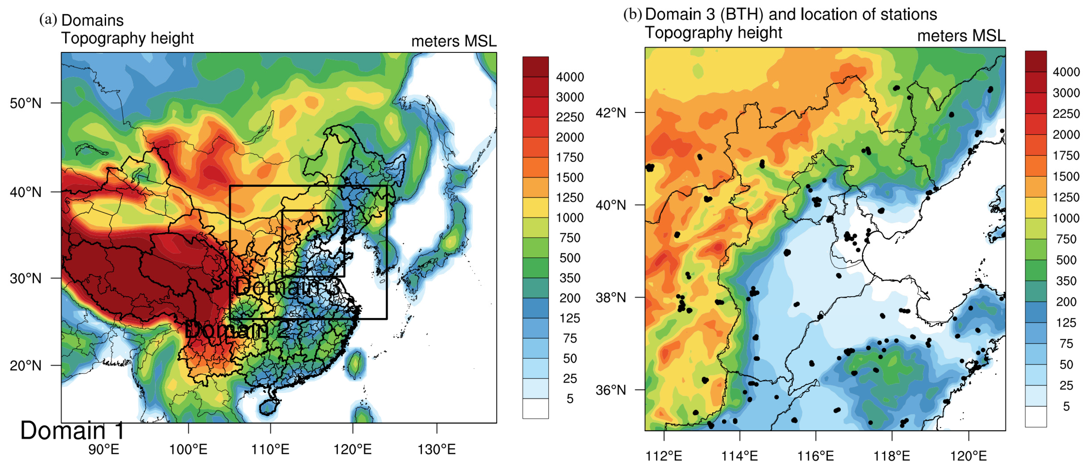
2.2. Model Configurations

This study applied a WRF-CMAQ modeling system to simulate the variations in PM2.5 and O3. The WRF was developed by the National Center for Atmospheric Research (NCAR) and the University Corporation for Atmospheric Research (UCAR) [30,31]. WRFv3.7.1 was used to generate the meteorological driver for the air quality simulation. The CMAQ modeling system is an active open-source development project of the United States Environmental Protection Agency, which consists of a suite of programs for model simulations of air quality [32]. We used CMAQv5.3.2 [33] to simulate the spatial distribution and temporal variation of the PM2.5, O3, and NO2 concentrations within the study region between 2 and 30 January 2019. All the simulations were restarted every 24 h, using the last simulation as the initial conditions and simulated 72 h concentration. There were 3 simulation cycle spin-ups before 2 January 2019. The boundary conditions of domain 1 and the initial conditions of the first simulation cycle used the mean value of the climate state. The detailed WRF-CMAQ model configurations are listed in Table A1 and Table A2. The model simulation domain and topographic height are shown in Figure 1.

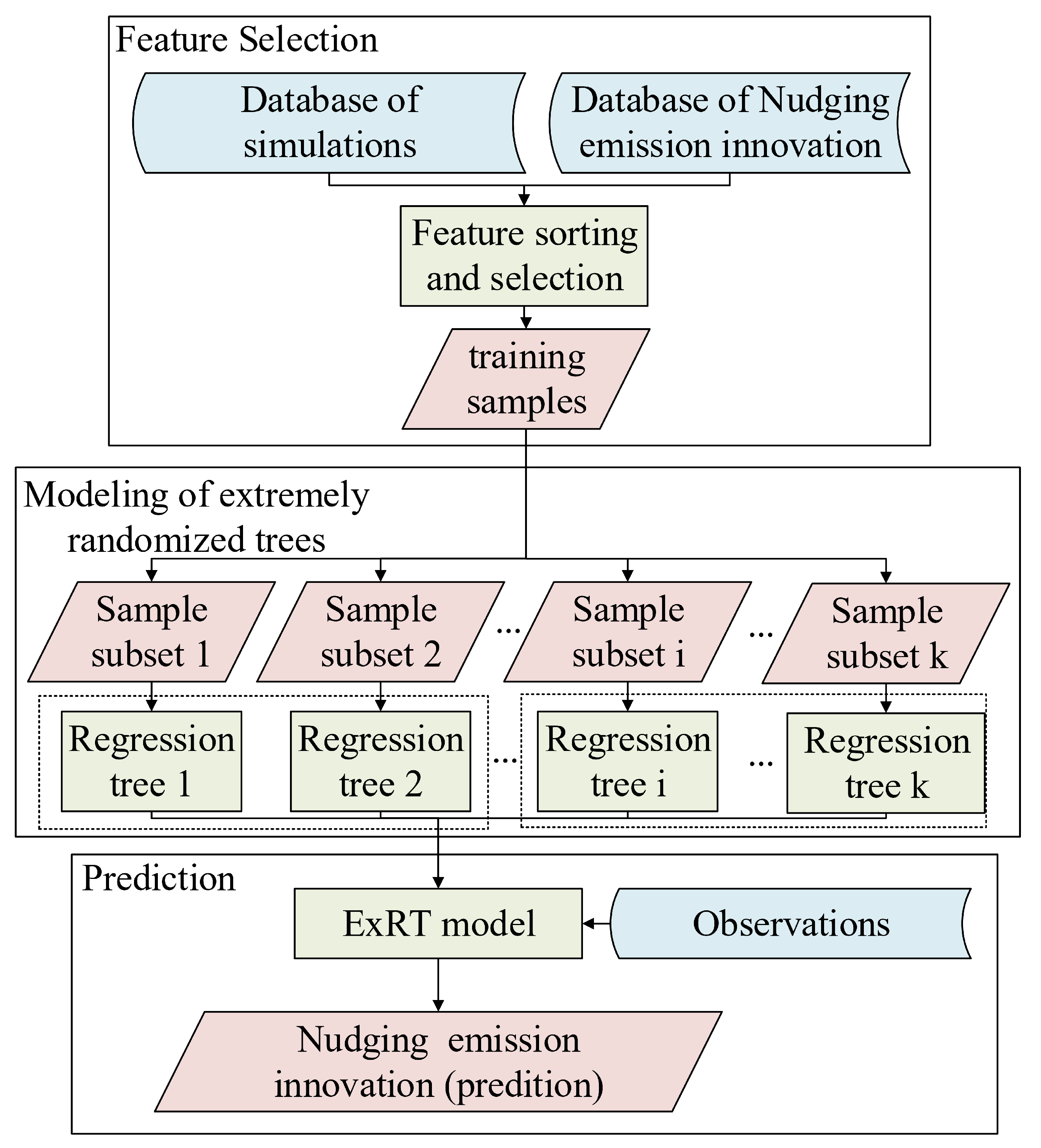
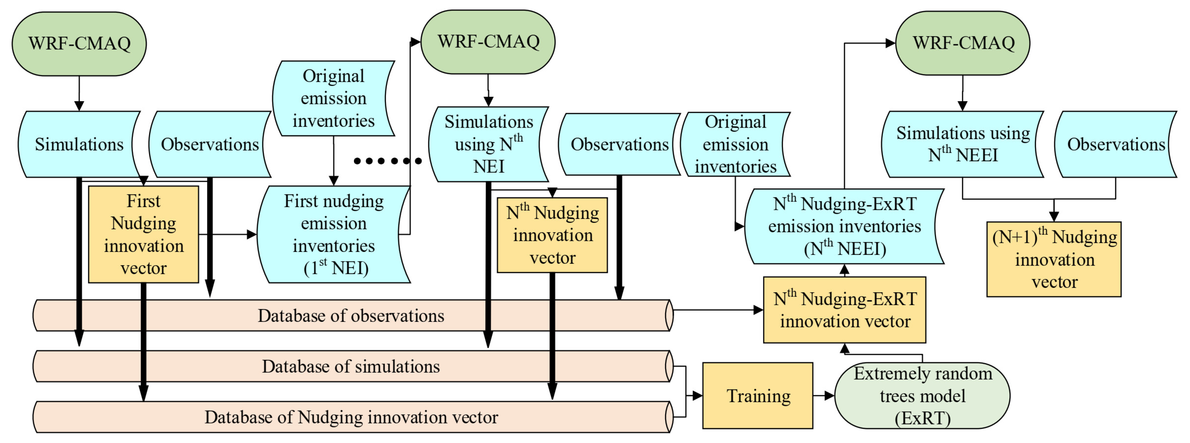
2.3. The Combination of Nudging and ExRT

The nudging method [34] has been widely used for improving air quality forecasting [18,19]. The nudging form can be expressed as
P n t = F P n , x , t + N ( P n , P * , Q * + Q n )
Q n + 1 = Q n × [ P * P n β P n P n 1 ] P n P n 1
Q n + 1 = Q * + Q n + 1
where P n is the concentration of the pollution in n iterations, t is the time, F is the array of the forcing function, N is the nudging terms, P * is the concentration of the observations, Q * is the original emission inventories, Q n is the emission innovation vector (the differences between the original emissions and assimilated emissions), and β is the empirical nudging coefficients.
The nudging used the original emissions ( Q * ), observations ( P * ), and simulated concentrations of the CMAQ ( P n ) to calculate the differences between the assimilated and original emissions (innovations) ( Q n + 1 ). Then, the assimilated emissions ( Q n + 1 ) were calculated using the emission innovations and original emissions to improve the CMAQ forecasts.
Firstly, the CMAQ predicted the concentration of P 1 , and the observed concentration of P 1 * and original emission data of Q 1 from the MEIC were used to derive the first emission innovation vector, Q 1 , Q 1 = β × Q 1 × [ P 1 * P 1 ] P 1 . Then, the new emission Q 2 = Q 1 + Q 1 was used to predict the concentration of P 2 using the CMAQ. P 1 and P 2 were used to estimate Q 2 using Equation (2). In this study, the iteration of the nudging went with the simulation circle, which meant that we only ran one nudging in a single simulation every 24 h.
While there were adequate data, we used all the simulations (the CMAQ-predicted concentrations) and corresponding emission innovation vectors in the database (which grew with the simulation circle) to train the ExRT model, and we used the trained ExRT model and the observations to calculate the prediction emission innovation vector. The training and prediction of the ExRT model can be expressed as:
Q 1 Q n = M n ( P 1,1 P n , 1 P 1 , s P n , s )
Q n + 1 = M n ( P 1,1 * P n , 1 * P 1 , s * P n , s * )
where M n is the ExRT model in simulation n, trained in Equation (4) and used in Equation (5); P n , s is the simulated concentration of the pollutant s in iteration n; and P n , s * is the observed concentration of the pollutant s in iteration n. As for PM2.5, s = 1, the PM2.5 emission innovations, Q n + 1 , were calculated using the simulated observed PM2.5 concentration and the corresponding PM2.5 emission innovations. As for the VOCs, s = 2, the VOC emission innovations were calculated using the simulated observed O3 and NO2 concentrations and the corresponding VOC emission innovations. The calculation of NOx was similar to that of the VOCs.
The extremely randomized trees method was developed by Geurts et al. [35], which is an improved version of the original decision tree models using the classical top-down procedure. A nonlinear solution can be found in the basic decision tree models. The entropy in probability theory is used in a decision tree to measure the uncertainty of information, and can be calculated as follows:
H X = i = 1 n p ( x i ) l o g b p ( x i )
where H(X) is the entropy of X, n is the number of samples, p ( x i ) is the probability that x i occurs, and l o g b p ( x i ) is the logarithm of p ( x i ) to base b.
Figure 2 shows the framework of the ExRT, and the construction of the ExRT is mainly divided into three parts. The first step was the feature selection. The database of simulations corresponded to the nudging emission innovations in the chronological order of spatial conversion, unit conversion, and chemical species. The entropy was automatically calculated and sorted to obtain the selected training samples. The second step was the modeling of the ExRT. In order to comprehensively train all of the samples and enhance the independence of the basic regression tree, part of the basic regression tree used all of the training samples, while the other part used the resampling training samples. If the input sample passed the given criteria, a leaf node was generated; otherwise, several candidate attributions were randomly calculated to generate several candidate sample subsets. When selecting the eigenvalues of the node splitting, the split was according to the attribute with the highest regression score, until the given criteria were met. The construction process of the k-times regression tree was repeated to form the ExRT model. The third step was the prediction, which was based on the ExRT model that was trained in the previous step and combined with the observations, and finally, the corresponding nudging emission innovation results were obtained.
The main innovations of the ExRT are as follows: (1) the randomly selected cut points are transformed into split nodes; and (2) the decision tree is constructed from the whole training dataset. This means that the ExRT generally does not use random sampling, and that each decision tree uses the original training samples. The partition points of the eigenvalues are randomly selected instead of using the most advantageous ones, and the size of the decision tree will generally be larger than the common random forest. In other words, the variance of the model is further reduced and the generalization ability, stability, and availability of the ExRT are better. A comparison of the ExRT, GBRT (gradient boosting regression tree), and MLS (multiple linear regression) was carried out in our previous MOS (model output statistics) study [28]. In a study of Xuzhou from 1 January 2016 to 31 March 2016, the WRF-CMAQ-MOS, using the ExRT, increased the correlation coefficient of the NO2 and O3 from 0.35 and 0.39 to 0.63 and 0.79, and the root mean square error decreased from 0.0346 mg/m3 and 0.0447 mg/m3 to 0.0243 mg/m3 and 0.0367 mg/m3. The scikit-learn machine learning package in Python was used here to accomplish the ExRT within nudging, and is available at http://scikit-learn.org/stable/index.html, accessed on 1 February 2022.
Figure 3 shows the framework of the nudging–ExRT methods that were used for the emission adjustment in the CMAQ. The nudging method was used to create a database of the nudging innovation vectors, using simulations of the CMAQ and ground-based observations. Then, these data were employed to train a machine learning model that used the ExRT, and to store the relationships between the nudging innovation vectors and the simulations in the trees. Using the trained machine learning model, the observations were used again to determine the proper nudging–ExRT innovation vector. The nudging–ExRT emission inventories were calculated using the original emission inventories and the nudging–ExRT innovation vector.
In the operational forecast of the emission data assimilation in the CMAQ simulation, we used nudging to calculate the hourly emission innovation vector between 2 and 14 January 2019, and created a database of the observations, simulations, and innovation vectors. Iterative nudging was performed every 24 h using all of the databases from the previous iterations to assimilate the emissions, and then used the assimilated emissions in the CMAQ to simulate the next 72 h of the pollutant concentrations. Then, we performed nudging (Nud) and nudging–ExRT (NudEx) experiments to adjust the anthropogenic emissions of the PM2.5, VOCs, and NOx between 15 and 30 January 2019. The proportion of the components did not change for PM2.5, VOCs, or NOx after the data assimilation. All the simulations of the PM2.5, O3, and NO2, and the innovation vectors of the emission database were used to train the machine learning model every 24 h. Finally, the machine learning model was used with the previous 72 h of observations to obtain the NudEx innovation vector for the next simulation. All the CMAQ simulations, including NODA (the CMAQ simulations without data assimilation), Nud, and NudEx, were restarted every 24 h, using the last simulation as their initial conditions. It should be noted that Nud could only use the database of O3 to adjust the emission of the VOCs, and that NudEx could use the databases of O3 and NO2 in the ExRT to adjust the emissions of the VOCs. As shown in Equations (1), (2), (4) and (5), the simulated concentration of the P n and the emission innovation of Q n were in a one-to-one correspondence for a pollutant species in Nud, and the VOC emission innovations were calculated by using the simulated observed O3 and NO2 concentrations and the corresponding VOC emission innovations in the NudEx.

3. Results

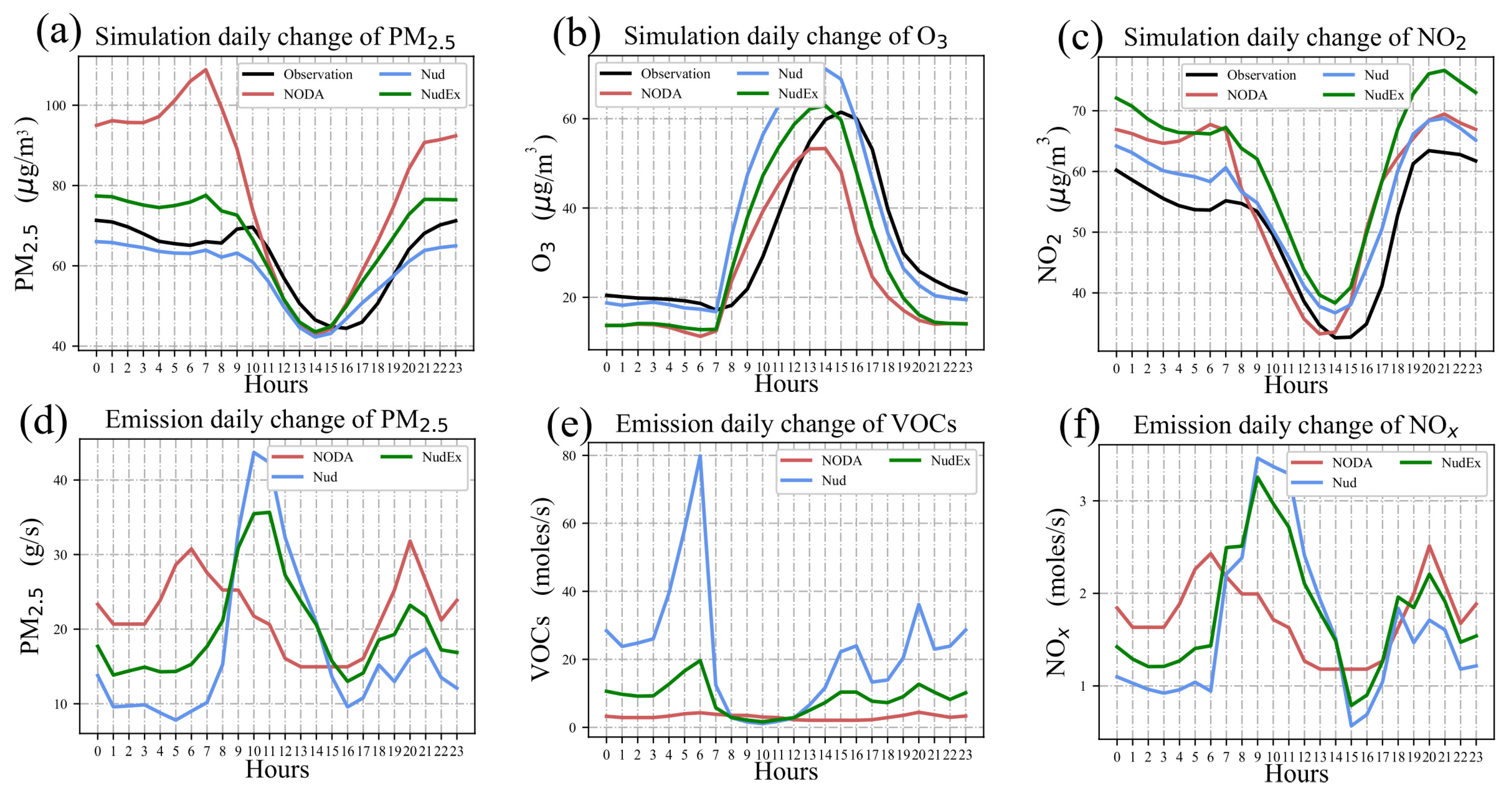
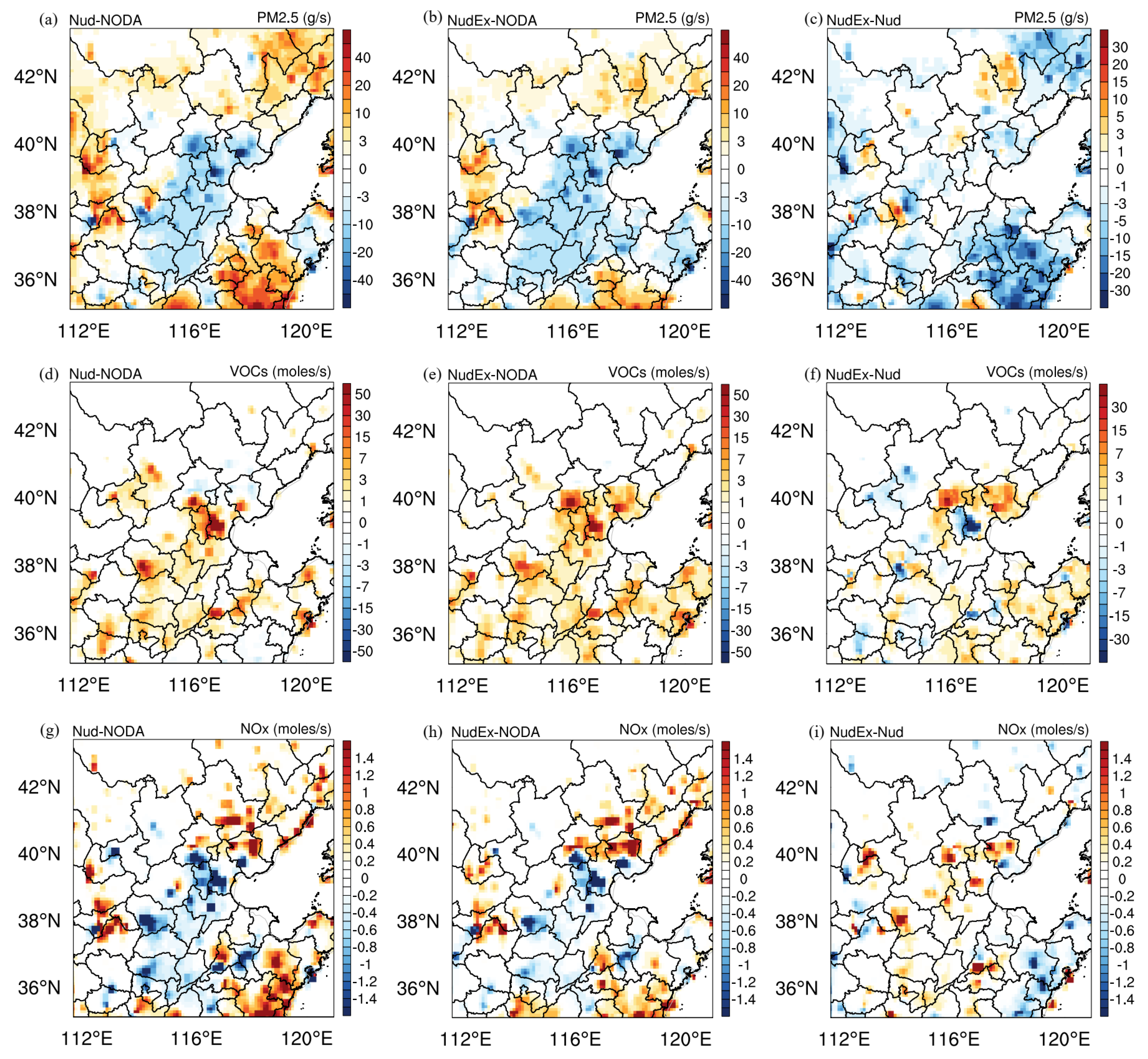
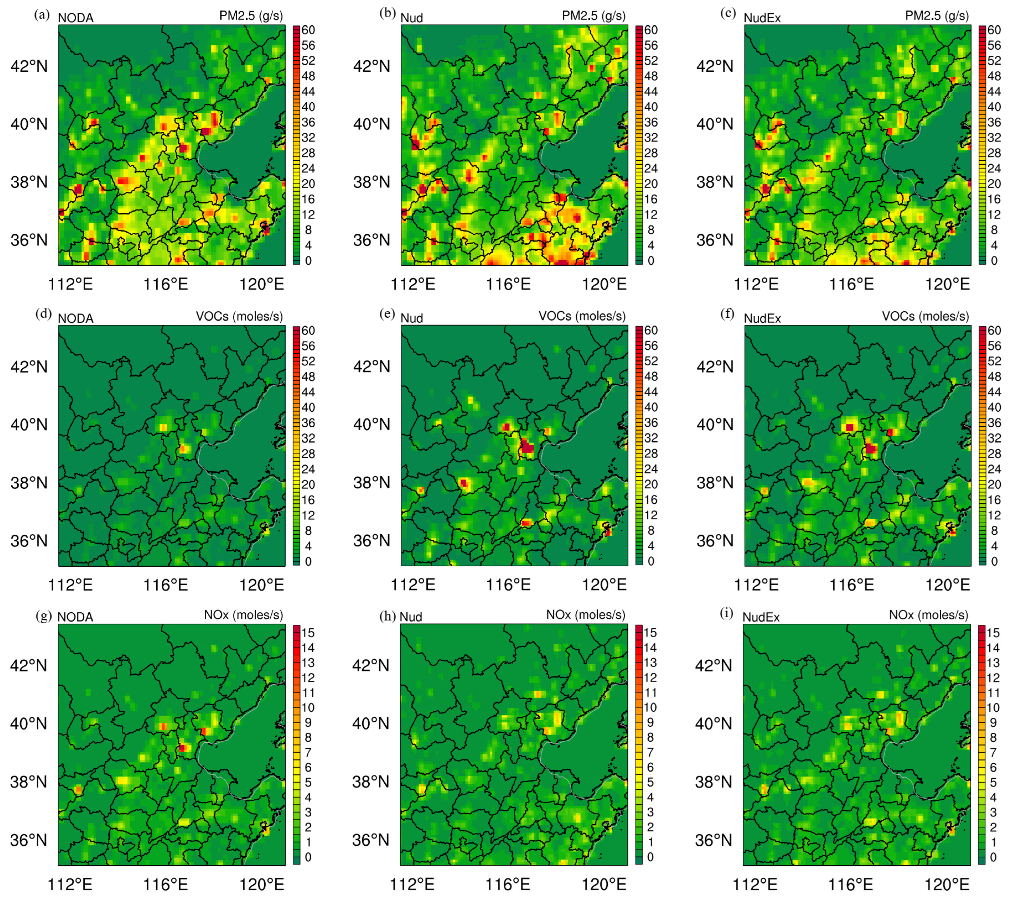
3.1. Anthropogenic Emission Adjustment

Figure 4 shows the daily change comparison in the NODA, Nud, and NudEx experiments of the PM2.5, O3, and NO2 concentrations and the PM2.5, VOC, and NOx emission inventories. The data in Figure 3 were calculated using the average of the 255 station locations in the BTH region and the 15 days between 15 and 30 January 2019. In Figure 3a, the daily change in the PM2.5 in the Nud and NudEx was closer to the observation than that of the NODA; meanwhile, the NudEx was closest around the leak at approximately 10 LST (Local Standard Time, UTC+8). In Figure 3b, the daily change in the O3 of the NudEx was closest to the observation around the leak at approximately 15 LST. The results expressed that the daily change in the NudEx emissions could better simulate the concentrations of PM2.5 and O3. All of the times used in this paper are expressed in LST.
Figure 5 shows the PM2.5, VOC, and NOx differences between the NODA, Nud, and NudEx emissions in the CMAQ as the hourly average of 15–30 January 2019. For the emission sources of PM2.5, the Nud reduced the emissions in Beijing and southern Hebei, and increased the emissions in western Shanxi, southeastern Liaoning, and western Shandong. The NudEx reduced the emissions in Beijing, southern Hebei, and northern Shandong. The largest differences between the Nud and NudEx were in Shandong and Liaoning. For the emission sources of the VOCs, Nud and NudEx both had an increasing tendency around Beijing, Tianjin, and Shijiazhuang. However, the NudEx had a larger adjustment in Beijing and a smaller adjustment in Tianjin and Shijiazhuang. For the emission sources of NOx, Nud and NudEx both had a decreasing tendency around Beijing and Tianjin, and had an increasing tendency in northeastern Hebei. The emissions of PM2.5, VOCs, and NOx in the NODA, Nud, and NudEx experiments can be found in Figure A1.

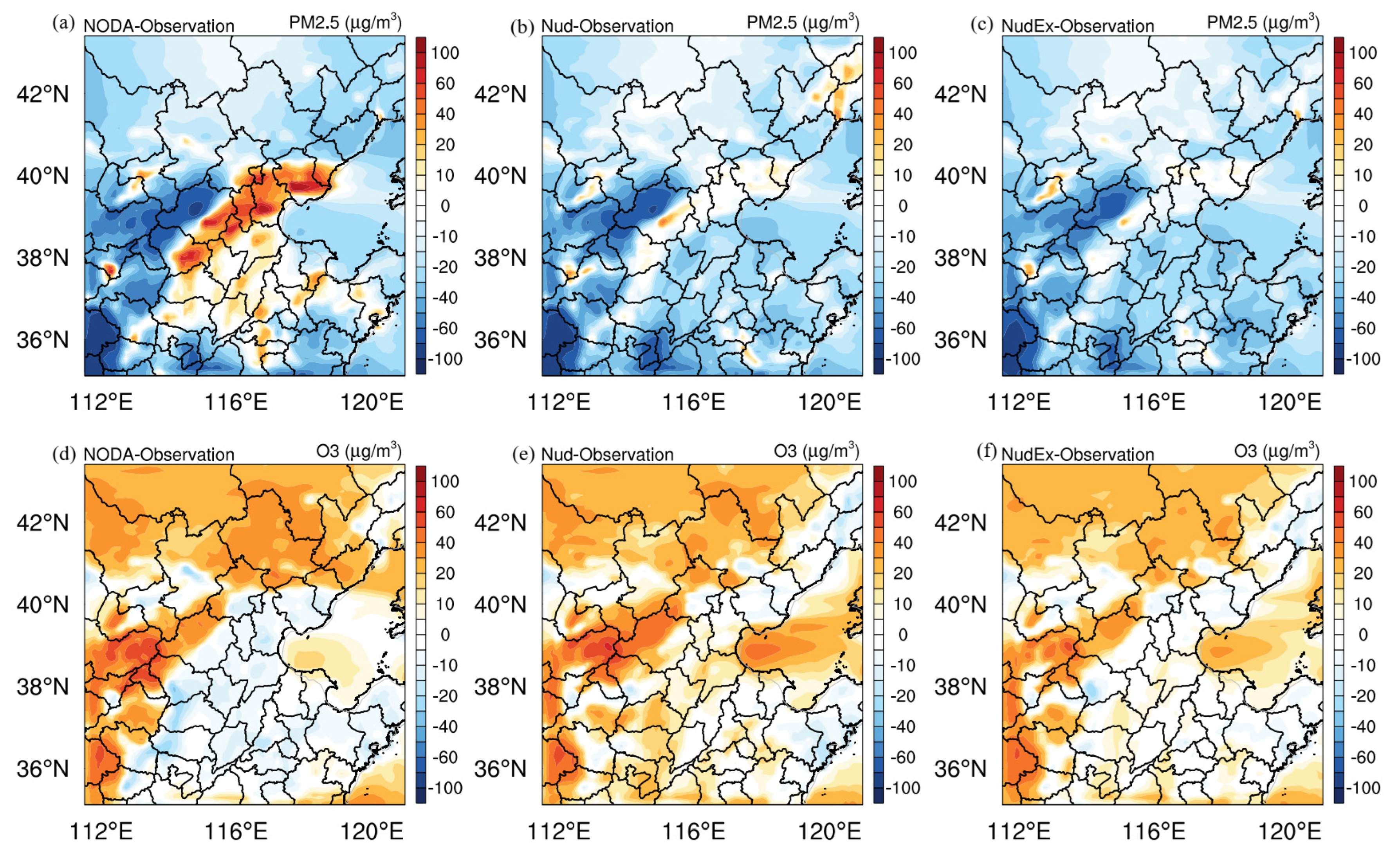
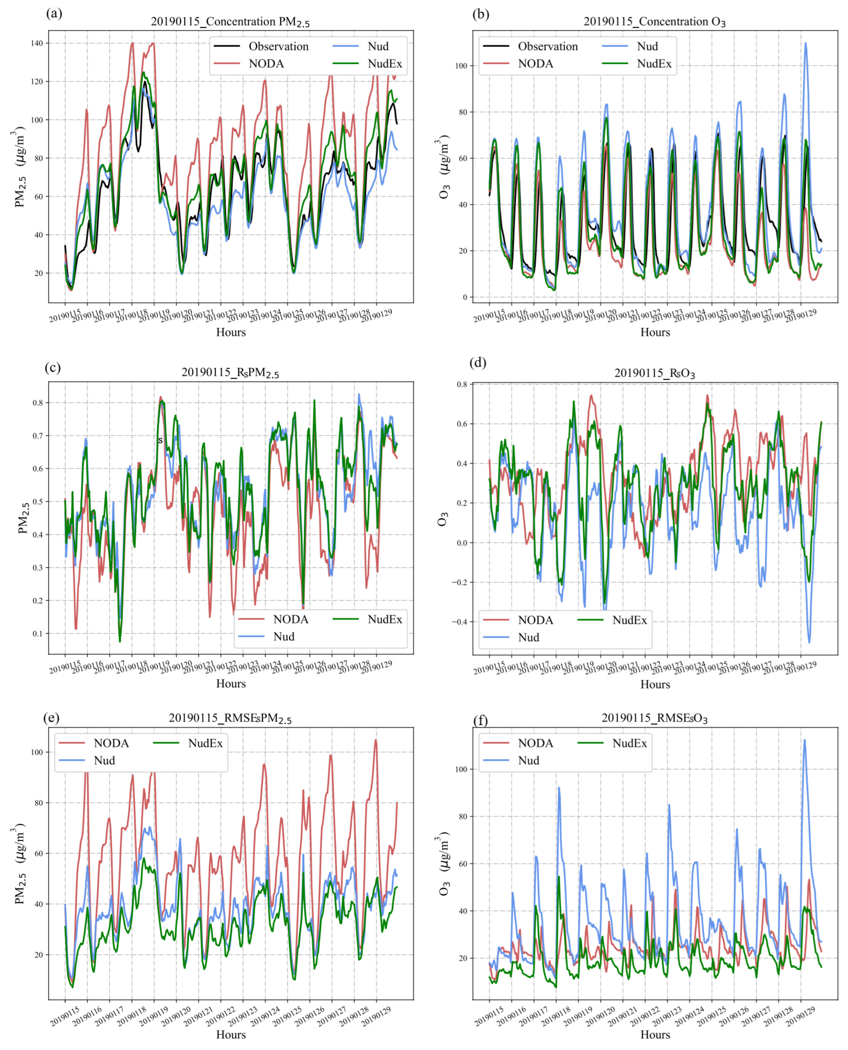
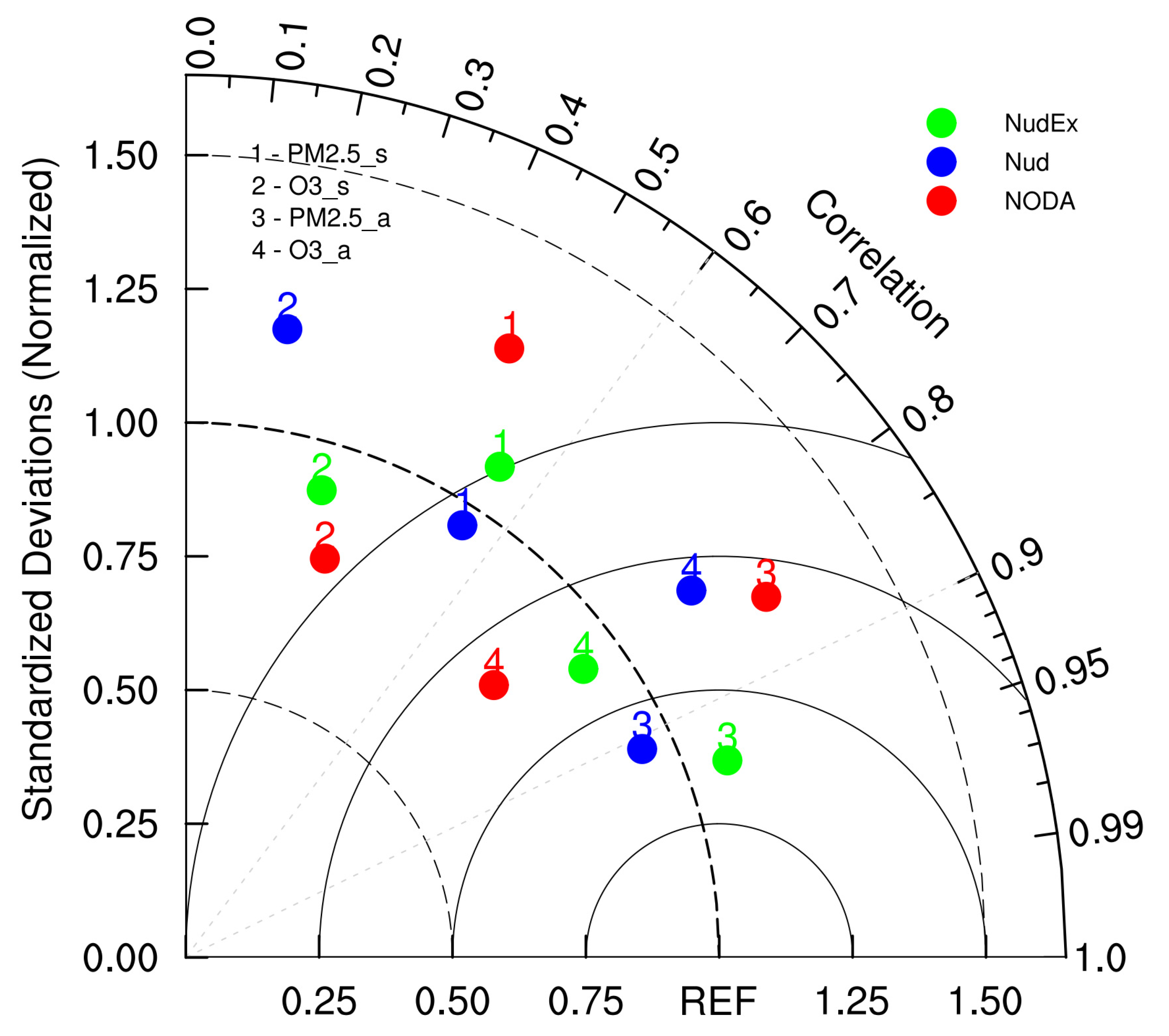
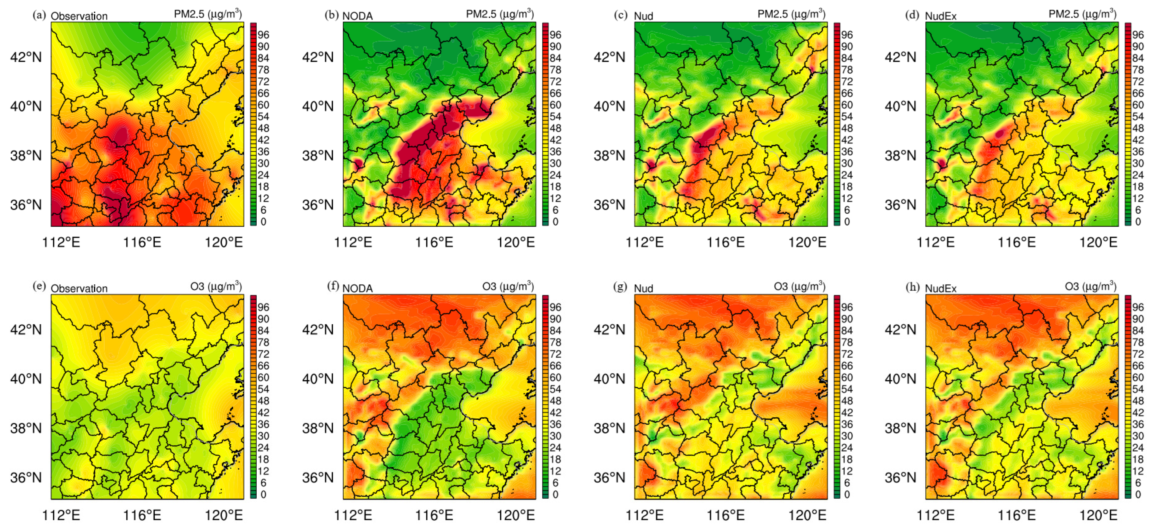
3.2. Emission Data Assimilation Results

Figure 6 shows the PM2.5 and O3 concentrations using the NODA, Nud, and NudEx emission inventories as the average of 15–30 January 2019. For PM2.5, the nudging methods could decrease the differences throughout the region, and NudEx had a better performance. For O3, owing to the fact that the Nud method was unable to deal with the nonlinear reaction of O3-VOCs-NOx, it had an even worse performance than NODA in the emission data assimilation of the VOCs. NudEx used machine learning methods and an increasing database to build a machine learning model of the observation, simulation, and emission innovations every 24 h. This machine learning model could partly replace the O3-VOCs-NOx nonlinear reactions in the emission data assimilation, using the existing O3 and NO2 observations to invert the emissions of the VOCs. These results showed that the nudging–ExRT method could improve the spatial accuracy of PM2.5 and O3 in the CMAQ. The concentrations of PM2.5 and O3 in the observations and the NODA, Nud, and NudEx experiments can be found in Figure A2.
To assess the performance of the NODA CMAQ simulation and the Nud and NudEx emission data assimilation results, the simulated PM2.5 and O3 concentrations were compared to the observations from the 255 air quality stations from the China National Environmental Monitoring Center. The hourly averaged spatial correlation coefficient ( R s ), hourly averaged spatial root mean squared error ( R M S E s ), hourly averaged spatial normalized mean bias ( N M B s ), hourly averaged spatial normalized mean error ( N M B s ), correlation coefficient of the site averaged concentration (Ra), root mean squared error of the site averaged concentration (RMSEa), normalized mean bias of the site averaged concentration (NMBa), and the normalized mean error of the site averaged concentration (NMEa) were used to validate the results. These statistical parameters were divided into two different types: spatial ( R s , R M S E s , N M B s , and N M B s ) and temporal (Ra, RMSEa, NMBa, and NMEa). The spatial statistics first calculated the statistical parameters for the 255 stations for each hour, and then calculated the average of these parameters. The temporal statistics first calculated the average for the 255 stations, and then used the averaged concentration to calculate the statistical parameters.
R s ( t ) = s = 1 m ( C ( t , s ) C ( t , s ) ) ( C 0 ( t , s ) C 0 ( t , s ) ) s = 1 m ( C ( t , s ) C ( t , s ) ) 2 s = 1 m ( C 0 ( t , s ) C 0 ( t , s ) ) 2
R M S E s ( t ) = s = 1 m ( C ( t , s ) C 0 ( t , s ) ) 2 m 1
N M B s ( t ) = s = 1 m ( C ( t , s ) C 0 ( t , s ) ) s = 1 m C 0 ( t , s ) × 100 %
N M E s ( t ) = s = 1 m C ( t , s ) C 0 ( t , s ) s = 1 m C 0 ( t , s ) × 100 %
R a = t = 1 n ( C a ( t ) C a ( t ) ) ( C 0 a ( t ) C 0 a ( t , m ) ) t = 1 n ( C a ( t ) C a ( t ) ) 2 t = 1 n ( C 0 a ( t ) C 0 a ( t , m ) ) 2
R M S E a = t = 1 n ( C a ( t ) C 0 a ( t ) ) 2 n 1
N M B a = t = 1 n ( C a ( t ) C 0 a ( t ) ) t = 1 n C 0 a ( t ) × 100 %
N M E a = t = 1 n C a ( t ) C 0 a ( t ) t = 1 n C 0 a ( t ) × 100 %
Here, C(n,m) is the simulated concentration matrix of n hours and m stations, C0(n,m) is the observed concentration matrix of n hours and m stations, R s ( t ) is the spatial correlation coefficient at time t, and R s = 1 n t = 1 n R s t . Similarly, R M S E s = 1 n t = 1 n R M S E s ( t ) , N M B s = 1 n t = 1 n N M B s ( t ) , and N M E s = 1 n t = 1 n N M E s ( t ) . C a ( t ) and C 0 a ( t ) are the site-averaged simulated and observed concentrations, respectively, and C a t = 1 m s = 1 m C t , s   a n d   C 0 a ( t ) = 1 m s = 1 m C 0 ( t , s ) .
Figure 7 and Table 1 show the assessments of PM2.5 and O3 in the NODA, Nud, and NudEx simulations. For PM2.5, all the assessments of the PM2.5 were improved in the Nud experiments and were better in the NudEx. For O3, the assessments of the O3 showed that the Nud decreased the correlation coefficient and increased the root mean squared error, which meant the Nud made the simulation worse. The reason for this was that the Nud reckoned without the nonlinear reactions of O3-VOCs-NOx and only considered the direct reaction between O3 and the VOCs. All the assessments, except the R s of the NudEx, showed a better performance for O3, and the NudEx could partly take the place of nonlinear reactions. The R s of the O3 in the NudEx decreased mainly because the low Rs at night were caused by the low O3 concentration after the assimilation. These results showed that the nudging–ExRT method could improve both the temporal and spatial accuracy of PM2.5 and O3 in the CMAQ.
Using the assessment data of the PM2.5 and O3, Figure 8 shows a Taylor diagram of the hourly averaged spatial and site-averaged PM2.5 and O3 comparison of the observations and simulations, using the NODA, Nud, and NudEx emission inventories in China between 15 and 30 January 2019. The scattered points in the Taylor chart represent the simulations using different emissions, the radiation line represents the correlation coefficient, and the horizontal and vertical axes represent the normalized standard deviation. These results directly point out that NudEx had more significant improvements than Nud.

4. Conclusions

In this paper, we established an efficient and extensible data assimilation method that was combined with machine learning to adjust the anthropogenic emissions in the CMAQ. The framework of nudging–ExRT was efficient, and the key point is that we only performed one iteration in every forecast and used all the data in the increasing database to build the machine learning model. In the experiment of this paper, a total of four Linux servers that were connected through optical fiber were used. Each server had two Intel (R) Xeon (R) E5-2620 v4 16-core CPUs, a total of 128 cores, 16 G of memory, 6 T of storage space, and 100 T of separate shared disk storage. It only took approximately half an hour before the forecasting and could be widely used for operational forecasting. The framework is extensible for adoption by other air quality models, because it only uses changeable emission sources and their corresponding simulations. The data assimilation and machine learning methods are both changeable and can be better extended in the future.
The results proved that the nudging method without the ExRT could improve the forecasting accuracy in linear emission sources, but could not eliminate nonlinear errors, and that the nudging–ExRT method, based on ensemble methods and probability theory, could significantly improve both the linear and nonlinear emission sources. We used O3 observations and simulations to adjust the VOC emissions in the Nud experiment. The nudging method attributed all of the errors in O3 to the VOCs, which was wrong, since it only considered the direct reaction between O3 and the VOCs. In the NudEx experiment, the machine learning model of the VOCs was established using O3 and NO2 observations and simulations. The ExRT model used the database to create the nonlinear relationships between the O3 and NO2 simulations and the VOC emissions, which could replace the real reactions. The reactions of the O3-VOCs-NOx in the CMAQ can be found in a study by Sarwar et al. [36].
This attempt to combine data assimilation and machine learning has proven to be a good way to invert both linear and nonlinear anthropogenic emission sources. In our experiments from 15 to 30 January 2019, in the BTH region of China, for the PM2.5, the R s increased from 0.47 to 0.54, the R M S E s decreased from 56.44 µg/m3 to 32.20 µg/m3, the Ra increased from 0.85 to 0.94, and the RMSEa decreased from 24.41 µg/m3 to 9.97 µg/m3. For the O3, the R s decreased from 0.33 to 0.28, the R M S E s decreased from 24.60 µg/m3 to 19.51 µg/m3, the Ra increased from 0.75 to 0.81, and the RMSEa decreased from 13.91 µg/m3 to 12.07 µg/m3. These results showed that the nudging–ExRT method could improve both the temporal and spatial accuracy of the PM2.5 and O3 in the CMAQ.
The results of the nudging–ExRT show good prospects for combining data assimilation and machine learning. This study can help researchers to gain more knowledge on the relationship between nonlinear emission sources and pollution. The accuracy of the operational air quality model can benefit from this framework and its extension.

Author Contributions

Conceptualization, C.H. and T.W.; methodology, C.H. and T.N.; software, C.H.; validation, C.H.; formal analysis, C.H.; investigation, C.H.; resources, M.L.; data curation, H.W. and H.L.; writing—original draft preparation, C.H.; writing—review and editing, T.W., T.N., Y.Q. and R.L.; visualization, C.H.; supervision, M.L.; project administration, T.W. and T.N.; funding acquisition, T.W. and T.N. All authors have read and agreed to the published version of the manuscript.

Funding

This research was funded by the National Key Basic Research and Development Program (No. 2019YFC0214603 and 2020YFA0607802), Basic Research Fund of CAMS (No. 2019Z014), the National Natural Science Foundation of China (No. 42077192 and 41975153), the National Key Basic Research and Development Program (No. 2022YFC3701105), the Research Funds for the Frontiers Science Center for Critical Earth Material Cycling, Nanjing University (No. 14380189) and supported by the program of CAEP “Analysis of the temporal and spatial changes in pollution meteorology and their dynamic impacts on air quality in 2020”.

Data Availability Statement

Observation data from 255 air quality stations in the Beijing–Tianjin–Hebei (BTH) region from the China National Environmental Monitoring Center were used and can be downloaded from http://www.cnemc.cn/en/, accessed on 15 March 2019. The FNL 1° × 1° data produced by the NCEP were used in this simulation to initialize the WRF, which can be downloaded from https://rda.ucar.edu/datasets/ds083.2/, accessed on 1 March 2020. Geographical input data, which provides static geographical data for WPS input, and can be downloaded from https://www2.mmm.ucar.edu/wrf/users/download/get_sources_wps_geog.html, accessed on 15 June 2019. The MEIC emission inventories can be downloaded from http://meicmodel.org/, accessed on 1 February 2022. CMAQv5.3.2 can be downloaded openly from https://github.com/USEPA/CMAQ/archive/5.3.2.zip, accessed on 1 September 2021. The scikit-learn machine learning package in Python was used here to accomplish ExRT in Nudging and is available at http://scikit-learn.org/stable/index.html, accessed on 1 February 2022.

Conflicts of Interest

The authors declare no conflict of interest.

Appendix A

Figure A1. The PM2.5, VOCs, and NOx emission intensity in the NODA, Nud, and NudEx experiments in the CMAQ as the hourly average from 15 to 30 January 2019: (a) NODA PM2.5; (b) Nud PM2.5; (c) NudEx PM2.5; (d) NODA VOCs; (e) Nud VOCs; (f) NudEx VOCs; (g) NODA NOx; (h) Nud NOx; and (i) NudEx NOx.
Remotesensing 15 01711 g0a1
Figure A2. The PM2.5 and O3 concentrations of the observations and using the NODA, Nud, and NudEx emission inventories averaged from 15 to 30 January 2019: (a) observation PM2.5; (b) NODA PM2.5; (c) Nud PM2.5; (d) NudEx PM2.5; (e) Observation O3; (f) NODA O3; (g) Nud O3; and (h) NudEx O3.
Remotesensing 15 01711 g0a2
Table A1. WRF simulation configurations.
WRFv3.7.1
Simulation period3–30 January 2019
Vertical resolution33 Vertical levels
Microphysics schemeWSM 3-class simple ice scheme [37]
Boundary layer schemeYSU scheme [38]
Surface layer schemeMM5 scheme [39]
Land-surface schemeUnified Noah land-surface model [40]
Longwave radiation schemerrtm scheme [41]
Shortwave radiation schemeDudhia scheme [42]
Grid-nudging fddaon
Domain center39.1248°N, 116.5657°E
Domain id123
Domain size64 × 7569 × 81102 × 96
Starting IJ-indices from the parent domain×(30, 19)(38, 23)
Horizontal resolution81 km27 km9 km
Table A2. CMAQ simulation configurations.
CMAQv5.3.2
Horizontal advectionYamo [32]
Vertical advectionWRF
Horizontal diffusionMultiscale
Vertical diffusionACM2
DepositionM3Dry [43]
Chemistry solverEBI
Aerosol moduleAERO7 [44]
Cloud moduleACM [45]
Mechanismcb6r3_ae7_aq [44,46]
Domain ID123
Domain size62 × 7367 × 79100 × 94

References

  1. Ministry of Ecology and Environment, The People’s Republic of China. Circular of the State Council on Printing Out and Distribution of the National “12th Five-Year Plan” for Environmental Protection. 2011. Available online: http://english.mee.gov.cn/Resources/Plans/National_Fiveyear_Plan/201606/P020160601356854927248.pdf (accessed on 1 May 2021).
  2. The State Council, The People’s Republic of China. Notice of the State Council on Printing and Distributing the Three-Year Action Plan for Winning the Blue Sky Protection Campaign. 2018. Available online: http://www.gov.cn/zhengce/content/2018-07/03/content_5303158.htm (accessed on 1 May 2021).
  3. Ma, Z.; Xu, J.; Quan, W.; Zhang, Z.; Lin, W.; Xu, X. Significant increase of surface ozone at a rural site, north of eastern China. Atmos. Chem. Phys. 2016, 16, 3969–3977. [Google Scholar] [CrossRef] [Green Version]
  4. Sun, L.; Xue, L.; Wang, T.; Gao, J.; Ding, A.; Cooper, O.R.; Lin, M.; Xu, P.; Wang, Z.; Wang, X.; et al. Significant increase of summertime ozone at Mount Tai in Central Eastern China. Atmos. Chem. Phys. 2016, 16, 10637–10650. [Google Scholar] [CrossRef] [Green Version]
  5. Wang, T.; Wei, X.L.; Ding, A.J.; Poon, C.N.; Lam, K.S.; Li, Y.S.; Chan, L.Y.; Anson, M. Increasing surface ozone concentrations in the background atmosphere of Southern China, 1994–2007. Atmos. Chem. Phys. 2009, 9, 6217–6227. [Google Scholar] [CrossRef] [Green Version]
  6. Xu, W.; Lin, W.; Xu, X.; Tang, J.; Huang, J.; Wu, H.; Zhang, X. Long-term trends of surface ozone and its influencing factors at the Mt Waliguan GAW station, China—Part 1: Overall trends and characteristics. Atmos. Chem. Phys. 2016, 16, 6191. [Google Scholar] [CrossRef] [Green Version]
  7. Han, C.L.; Xu, R.B.; Zhang, Y.J.; Yu, W.H.; Zhang, Z.W.; Morawska, L.; Heyworth, J.; Jalaludin, B.; Morgan, G.; Marks, G.; et al. Air pollution control efficacy and health impacts: A global observational study from 2000 to 2016. Environ. Pollut. 2021, 287, 117211. [Google Scholar] [CrossRef] [PubMed]
  8. Hu, F.; Guo, Y. Health impacts of air pollution in China. Front. Environ. Sci. Eng. 2021, 15, 1–8. [Google Scholar] [CrossRef]
  9. Shen, W.T.; Yu, X.; Zhong, S.B.; Ge, H.R. Population Health Effects of Air Pollution: Fresh Evidence From China Health and Retirement Longitudinal Survey. Front. Public Health 2021, 9, 1620. [Google Scholar] [CrossRef]
  10. Cao, G.L.; Zhang, X.Y.; Gong, S.L.; An, X.Q.; Wang, Y.Q. Emission inventories of primary particles and pollutant gases for China. Chin. Sci. Bull. 2011, 56, 781–788. [Google Scholar] [CrossRef] [Green Version]
  11. Streets, D.G.; Bond, T.C.; Carmichael, G.R.; Fernandes, S.D.; Fu, Q.; He, D.; Klimont, Z.; Nelson, S.M.; Tsai, N.Y.; Wang, M.Q.; et al. An inventory of gaseous and primary aerosol emissions in Asia in the year 2000. J. Geophys. Res.-Atmos. 2003, 108. [Google Scholar] [CrossRef]
  12. Zhang, Q.; Streets, D.G.; Carmichael, G.R.; He, K.B.; Huo, H.; Kannari, A.; Klimont, Z.; Park, I.S.; Reddy, S.; Fu, J.S.; et al. Asian emissions in 2006 for the NASA INTEX-B mission. Atmos. Chem. Phys. 2009, 9, 5131–5153. [Google Scholar] [CrossRef] [Green Version]
  13. Zhao, B.; Wang, P.; Ma, J.Z.; Zhu, S.; Pozzer, A.; Li, W. A high-resolution emission inventory of primary pollutants for the Huabei region, China. Atmos. Chem. Phys. 2012, 12, 481–501. [Google Scholar] [CrossRef] [Green Version]
  14. Kasibhatla, P.; Arellano, A.; Logan, J.A.; Palmer, P.I.; Novelli, P. Top-down estimate of a large source of atmospheric carbon monoxide associated with fuel combustion in Asia. Geophys. Res. Lett. 2002, 29, 6-1. [Google Scholar] [CrossRef] [Green Version]
  15. Mo, Z.; Shao, M.; Liu, Y.; Xiang, Y.; Wang, M.; Lu, S.; Ou, J.; Zheng, J.; Li, M.; Zhang, Q.; et al. Species-specified VOC emissions derived from a gridded study in the Pearl River Delta, China. Sci. Rep. 2018, 8, 2963. [Google Scholar] [CrossRef] [Green Version]
  16. Trombetti, M.; Thunis, P.; Bessagnet, B.; Clappier, A.; Couvidat, F.; Guevara, M.; Kuenen, J.; López-Aparicio, S. Spatial inter-comparison of Top-down emission inventories in European urban areas. Atmos. Environ. 2018, 173, 142–156. [Google Scholar] [CrossRef]
  17. Van Vuuren, D.P.; Hoogwijk, M.; Barker, T.; Riahi, K.; Boeters, S.; Chateau, J.; Scrieciu, S.; van Vliet, J.; Masui, T.; Blok, K.; et al. Comparison of top-down and bottom-up estimates of sectoral and regional greenhouse gas emission reduction potentials. Energy Policy 2009, 37, 5125–5139. [Google Scholar] [CrossRef]
  18. Cheng, X.H.; Xu, X.D.; Ding, G.A. An emission source inversion model based on satellite data and its application in air quality forecasts. Sci. China-Earth Sci. 2010, 53, 752–762. [Google Scholar] [CrossRef]
  19. Xu, X.D.; Xie, L.; Cheng, X.H.; Xu, J.M.; Zhou, X.J.; Ding, G.A. Application of an adaptive nudging scheme in air quality forecasting in China. J. Appl. Meteorol. Climatol. 2008, 47, 2105–2114. [Google Scholar] [CrossRef]
  20. Tang, X.; Zhu, J.; Wang, Z.; Gbaguidi, A.; Lin, C.; Xin, J.; Song, T.; Hu, B. Limitations of ozone data assimilation with adjustment of NOx emissions: Mixed effects on NO2 forecasts over Beijing and surrounding areas. Atmos. Chem. Phys. 2016, 16, 6395–6405. [Google Scholar] [CrossRef] [Green Version]
  21. Mizzi, A.P.; Arellano, A.F.; Edwards, D.P.; Anderson, J.L.; Pfister, G.G. Assimilating compact phase space retrievals of atmospheric composition with WRF-Chem/DART: A regional chemical transport/ensemble Kalman filter data assimilation system. Geosci. Model Dev. 2016, 9, 965–978. [Google Scholar] [CrossRef] [Green Version]
  22. Peng, Z.; Lei, L.; Liu, Z.; Sun, J.; Ding, A.; Ban, J.; Chen, D.; Kou, X.; Chu, K. The impact of multi-species surface chemical observation assimilation on air quality forecasts in China. Atmos. Chem. Phys. 2018, 18, 17387–17404. [Google Scholar] [CrossRef] [Green Version]
  23. Ma, C.; Wang, T.; Jiang, Z.; Wu, H.; Zhao, M.; Zhuang, B.; Li, S.; Xie, M.; Li, M.; Liu, J.; et al. Importance of bias correction in data assimilation of multiple observations over eastern China using WRF-Chem/DART. J. Geophys. Res. Atmos. 2020, 125, e2019JD031465. [Google Scholar] [CrossRef]
  24. Ma, C.; Wang, T.; Mizzi, A.P.; Anderson, J.L.; Zhuang, B.; Xie, M.; Wu, R. Multiconstituent Data Assimilation With WRFChem/DART: Potential for Adjusting Anthropogenic Emissions and Improving Air Quality Forecasts Over Eastern China. J. Geophys. Res. Atmos. 2019, 124, 7393–7412. [Google Scholar] [CrossRef]
  25. Eslami, E.; Salman, A.K.; Choi, Y.; Sayeed, A.; Lops, Y. A data ensemble approach for real-time air quality forecasting using extremely randomized trees and deep neural networks. Neural Comput. Appl. 2020, 32, 7563–7579. [Google Scholar] [CrossRef]
  26. Tang, M.Z.; Chen, Y.T.; Wu, H.W.; Zhao, Q.; Long, W.; Sheng, V.S.; Yi, J.B. Cost-Sensitive Extremely Randomized Trees Algorithm for Online Fault Detection of Wind Turbine Generators. Front. Energy Res. 2021, 9, 234. [Google Scholar] [CrossRef]
  27. Xia, B.; Zhang, H.; Li, Q.M.; Li, T. PETs: A Stable and Accurate Predictor of Protein-Protein Interacting Sites Based on Extremely-Randomized Trees. IEEE Trans. Nanobiosci. 2015, 14, 882–893. [Google Scholar] [CrossRef]
  28. Huang, C.W.; Chen, B.Z.; Ma, C.Q.; Wang, T.J. WRF-CMAQ-MOS studies based on extremely randomized trees. Acta Meterologica Sin. 2018, 76, 779–789. [Google Scholar] [CrossRef]
  29. National Centers for Environmental Prediction; National Weather Service; NOAA; U.S. Department of Commerce. NCEP FNL Operational Model Global Tropospheric Analyses, Continuing from July 1999; Updated Daily; Research Data Archive at the National Center for Atmospheric Research, Computational and Information Systems Laboratory; National Centers for Environmental Prediction: College Park, MD, USA, 2000. [Google Scholar] [CrossRef]
  30. Skamarock, W.C.; Klemp, J.B.; Dudhia, J.; Gill, D.O.; Barker, D.M.; Duda, M.G.; Huang, X.-Y.; Wang, W.; Powers, J.G. A Description of the Advanced Research WRF Version 3; NCAR Tech.: Boulder, CO, USA, 2008. [Google Scholar] [CrossRef]
  31. Chen SY, S.; Price, J.F.; Zhao, W.; Donelan, M.A.; Walsh, E.J. The CBLAST-hurricane program and the next-generation fully coupled atmosphere-wave-ocean. Models for hurricane research and prediction. Bull. Am. Meteorol. Soc. 2007, 88, 311–317. [Google Scholar] [CrossRef]
  32. Byun, D.; Schere, K.L. Review of the governing equations, computational algorithms, and other components of the models-3 Community Multiscale Air Quality (CMAQ) modeling system. Appl. Mech. Rev. 2006, 59, 51–77. [Google Scholar] [CrossRef]
  33. United States Environmental Protection Agency. CMAQ (Version 5.3.2) [Software]; United States Environmental Protection Agency: Washington, DC, USA, 2020. [Google Scholar] [CrossRef]
  34. Hoke, J.E.; Anthes, R.A. The initialization of numerical models by a dynamic-initialization technique. Mon. Weather Rev. 1976, 104, 1551–1556. [Google Scholar] [CrossRef]
  35. Geurts, P.; Ernst, D.; Wehenkel, L. Extremely randomized trees. Mach. Learn. 2006, 63, 3–42. [Google Scholar] [CrossRef] [Green Version]
  36. Sarwar, G.; Luecken, D.; Yarwood, G.; Whitten, G.Z.; Carter, W.P.L. Impact of an updated carbon bond mechanism on predictions from the CMAQ modeling system: Preliminary assessment. J. Appl. Meteorol. Climatol. 2008, 47, 3–14. [Google Scholar] [CrossRef]
  37. Hong, S.Y.; Dudhia, J.; Chen, S.H. A Revised Approach to Ice Microphysical Processes for the Bulk Parameterization of Clouds and Precipitation. Mon. Weather Rev. 2004, 132, 103–120. [Google Scholar] [CrossRef]
  38. Hong, S.Y.; Noh, Y.; Dudhia, J. A new vertical diffusion package with an explicit treatment of entrainment processes. Mon. Weather Rev. 2006, 134, 2318–2341. [Google Scholar] [CrossRef] [Green Version]
  39. Paulson, C.A. The mathematical representation of wind speed and temperature profiles in the unstable atmospheric surface layer. J. Appl. Meteorol. 1970, 9, 857–861. [Google Scholar] [CrossRef]
  40. Chen, F.; Dudhia, J. Coupling an advanced land-surface/hydrology model with the Penn State/NCAR MM5 modeling system. Part I: Model description and implementation. Mon. Weather Rev. 2001, 129, 569–585. [Google Scholar] [CrossRef]
  41. Mlawer, E.J.; Taubman, S.J.; Brown, P.D.; Iacono, M.J.; Clough, S.A. Radiative transfer for inhomogeneous atmosphere: RRTM, a validated correlated-k model for the longwave. J. Geophys. Res. 1997, 102, 16663–16682. [Google Scholar] [CrossRef] [Green Version]
  42. Dudhia, J. Numerical study of convection observed during the winter monsoon experiment using a mesoscale two-dimensional model. J. Atmos. Sci. 1989, 46, 3077–3107. [Google Scholar] [CrossRef]
  43. Shu, Q.; Murphy, B.N.; Schwede, D.; Henderson, B.H.; Pye HO, T.; Appel, K.W.; Khan, T.R.; Perlinger, J.A. Improving the particle dry deposition scheme in the CMAQ photochemical modeling system. Atmos. Environ. 2022, 289, 119343. [Google Scholar] [CrossRef]
  44. Xu, L.; Pye HO, T.; He, J.; Chen, Y.L.; Murphy, B.N.; Ng, N.L. Experimental and model estimates of the contributions from biogenic monoterpenes and sesquiterpenes to secondary organic aerosol in the southeastern United States. Atmos. Chem. Phys. 2018, 18, 12613–12637. [Google Scholar] [CrossRef] [Green Version]
  45. Fahey, K.M.; Carlton, A.G.; Pye, H.O.T.; Baek, J.; Hutzell, W.T.; Stanier, C.O.; Baker, K.R.; Appel, K.W.; Jaoui, M.; Offenberg, J.H. A framework for expanding aqueous chemistry in the Community Multiscale Air Quality (CMAQ) model version 5.1. Geosci. Model Dev. 2017, 10, 1587–1605. [Google Scholar] [CrossRef] [Green Version]
  46. Luecken, D.J.; Yarwood, G.; Hutzell, W.H. Multipollutant of ozone, reactive nitrogen and HAPs across the continental US with CMAQ-CB6. Atmos. Environ. 2019, 201, 62–72. [Google Scholar] [CrossRef] [PubMed]
Figure 1. Simulation domains: (a) domains 1–3 and topography height; and (b) domain 3 (BTH) and locations of the stations.
Remotesensing 15 01711 g001
Figure 2. The framework of the ExRT.
Remotesensing 15 01711 g002
Figure 3. The framework of the nudging–ExRT method in CMAQ.
Remotesensing 15 01711 g003
Figure 4. The daily change comparison in the NODA, Nud, and NudEx experiments of the (a) PM2.5, (b) O3, and (c) NO2 concentrations, and the (d) PM2.5, (e) VOCs, and (f) NOx emission inventories.
Remotesensing 15 01711 g004
Figure 5. The PM2.5, VOCs, and NOx differences between the NODA, Nud, and NudEx emissions in the CMAQ as the hourly average of 15–30 January 2019: (a) Nud−NODA of PM2.5; (b) NudEx−NODA of PM2.5; (c) NudEx−Nud of PM2.5; (d) Nud−NODA of VOCs; (e) NudEx−NODA of VOCs; (f) NudEx−Nud of VOCs; (g) Nud−NODA of NOx; (h) NudEx−NODA of NOx; and (i) NudEx−Nud of PM2.5.
Remotesensing 15 01711 g005
Figure 6. The PM2.5 and O3 concentration differences using the NODA, Nud, and NudEx emission inventories and observations as the average of 15–30 January 2019: (a) NODA−observation of PM2.5; (b) Nud−observation of PM2.5; (c) NudEx−observation of PM2.5; (d) NODA−observation of O3; (e) Nud−observation of O3; and (f) NudEx−observation of O3.
Remotesensing 15 01711 g006
Figure 7. The PM2.5 and O3 comparison of the observations and simulations using NODA, Nud, and NudEx emission inventories in BTH between 15 and 30 January 2019: (a) concentration of the spatially averaged PM2.5; (b) concentration of the spatially averaged O3; (c) Rs of PM2.5; (d) Rs of O3; (e) RMSEs of PM2.5; and (f) RMSEs of O3.
Remotesensing 15 01711 g007
Figure 8. The Taylor diagram of the hourly averaged spatial (PM2.5_s and O3_s) and site-averaged (PM2.5_a and O3_a) comparison of the observations and simulations using the NODA, Nud, and NudEx emission inventories in BTH between 15 and 30 January 2019.
Remotesensing 15 01711 g008
Table 1. Assessment of PM2.5 and O3 in the NODA, Nud, and NudEx simulations.
PM2.5O3
NODANudNudExNODANudNudEx
R s 0.470.540.540.330.160.28
R M S E s
(µg/m3)
56.4438.2332.224.636.6119.51
N M B s 29%−4%9%−21%19%−9%
N M E s 67%44%47%72%92%74%
R a 0.850.910.940.750.810.81
R M S E a
(µg/m3)
24.4110.599.9713.9114.8612.07
N M B a 28%−6%8%−23%17%−8%
N M E a 32%13%13%33%31%31%
Disclaimer/Publisher’s Note: The statements, opinions and data contained in all publications are solely those of the individual author(s) and contributor(s) and not of MDPI and/or the editor(s). MDPI and/or the editor(s) disclaim responsibility for any injury to people or property resulting from any ideas, methods, instructions or products referred to in the content.

