Article

Above- and Belowground Biomass Carbon Stock and Net Primary Productivity Maps for Tidal Herbaceous Marshes of the United States

by
Victoria L. Woltz
1,*,
Camille LaFosse Stagg
2,
Kristin B. Byrd
3,
Lisamarie Windham-Myers
4,
Andre S. Rovai
5 and
Zhiliang Zhu
6
1
Cherokee Nation System Solutions Contractor to the U.S. Geological Survey, Wetland and Aquatic Research Center, Lafayette, LA 70506, USA
2
U.S. Geological Survey, Wetland and Aquatic Research Center, Lafayette, LA 70506, USA
3
U.S. Geological Survey, Western Geographic Science Center, Moffett Field, CA 94035, USA
4
U.S. Geological Survey, Water Resources Mission Area, Menlo Park, CA 94025, USA
5
Department of Oceanography and Coastal Sciences, College of the Coast and Environment, Louisiana State University, Baton Rouge, LA 70803, USA
6
U.S. Geological Survey, Ecosystems Mission Area, Reston, VA 20192, USA
*
Author to whom correspondence should be addressed.
Remote Sens. 2023, 15(6), 1697; https://doi.org/10.3390/rs15061697
Submission received: 14 January 2023 / Revised: 9 March 2023 / Accepted: 20 March 2023 / Published: 21 March 2023
(This article belongs to the Special Issue Use of Remote Sensing in Valuation of Blue Carbon and Its Co-benefits)

Abstract

:
Accurate assessments of greenhouse gas emissions and carbon sequestration in natural ecosystems are necessary to develop climate mitigation strategies. Regional and national-level assessments of carbon sequestration require high-resolution data to be available for large areas, increasing the need for remote sensing products that quantify carbon stocks and fluxes. The Intergovernmental Panel on Climate Change (IPCC) provides guidelines on how to quantify carbon flux using land cover land change and biomass carbon stock information. Net primary productivity (NPP), carbon uptake, and storage in vegetation, can also be used to model net carbon sequestration and net carbon export from an ecosystem (net ecosystem carbon balance). While biomass and NPP map products for terrestrial ecosystems are available, there are currently no conterminous United States (CONUS) biomass carbon stock or NPP maps for tidal herbaceous marshes. In this study, we used peak soil adjusted vegetation index (SAVI) values, derived from Landsat 8 composites, and five other vegetation indices, plus a categorical variable for the CONUS region (Pacific Northwest, California, Northeast, Mid-Atlantic, South Atlantic-Gulf, or Everglades), to model spatially explicit aboveground peak biomass stocks in tidal marshes (i.e., tidal palustrine and estuarine herbaceous marshes) for the first time. Tidal marsh carbon conversion factors, root-to-shoot ratios, and vegetation turnover rates, were compiled from the literature and used to convert peak aboveground biomass to peak total (above- and belowground) biomass and NPP. An extensive literature search for aboveground turnover rates produced sparse and variable values; therefore, we used an informed assumption of a turnover rate of one crop per year for all CONUS tidal marshes. Due to the lack of turnover rate data, the NPP map is identical to the peak biomass carbon stock map. In reality, it is probable that turnover rate varies by region, given seasonal length differences; however, the NPP map provides the best available information on spatially explicit CONUS tidal marsh NPP. This study identifies gaps in the scientific knowledge, to support future studies in addressing this lack of turnover data. Across CONUS, average total peak biomass carbon stock in tidal marshes was 848 g C m−2 (871 g C m−2 in palustrine and 838 g C m−2 in estuarine marshes), and based on a median biomass turnover rate of 1, it is expected that the mean NPP annual flux for tidal marshes is similar (e.g., 848 g C m−2 y−1). Peak biomass carbon stocks in tidal marshes were lowest in the Florida Everglades region and highest in the California regions. These are the first fine-scale national maps of biomass carbon and NPP for tidal wetlands, spanning all of CONUS. These estimates of CONUS total peak biomass carbon stocks and NPP rates for tidal marshes can support regional- and national-scale assessments of greenhouse gas emissions, as well as natural resource management of coastal wetlands, as part of nature-based climate solution efforts.

1. Introduction

As atmospheric carbon dioxide (CO2) concentrations continue to increase, global temperatures are approaching a threshold that will have irreversible consequences for the future of our planet [1]. To avoid the 2 °C warming threshold, policies aimed at reducing greenhouse gas emissions will rely in part on nature-based climate solutions, that enhance carbon storage and sequestration in ecosystems such as forests, grasslands, and wetlands [2]. Globally, long-term carbon sequestration in vegetated coastal habitats is much greater than that in terrestrial forests, despite the fact that their area is one to two orders of magnitude smaller [3,4]. Because coastal wetlands store large amounts of carbon in flooded soils, avoiding loss of coastal herbaceous marsh carbon stocks, and maintaining ecosystem rates of carbon sequestration via restoration and management, are becoming increasingly important tools for reducing net greenhouse gas emissions and mitigating climate change [5].
However, coastal wetlands are also vulnerable to changes in climate and land use [6]. In addition to salinity and flooding stress from sea-level rise [7,8], hydrologic alterations associated with both extreme precipitation and extreme drought can inhibit wetland plant production, and even cause complete mortality and ecosystem collapse [9,10]. Furthermore, coastal wetlands that are located at the upper limit of their tidal range are threatened directly and indirectly by land use drivers that alter geomorphic processes, including development of cities, ports, dams, dikes, and dredging and filling [11,12]. Carbon accounting in herbaceous marshes is important, as they represent 80 percent of all tidal wetlands in the conterminous U.S. (CONUS) [13]. Together, stressors from both climate and land use change have resulted in high rates of wetland loss [14], which, if not mitigated, could significantly contribute to additional U.S. greenhouse gas emissions [15]. Therefore, accounting for changes in coastal wetland area, and associated changes in carbon stocks and fluxes, in national-scale assessments of greenhouse gas emissions, as well as climate mitigation strategies that utilize nature-based climate solutions, can help to inform future land management.
Although recent U.S. National Greenhouse Gas (GHG) Inventories do provide tabular country-specific (IPCC Tier 2) estimates of coastal wetland emissions and reductions based on land cover data [16], spatially explicit assessments of coastal wetland carbon sequestration (or emissions) are not available at the national scale. A key limitation to this effort is the availability of spatially explicit wetland carbon data, including biomass carbon stocks and net primary production (NPP) fluxes of wetland vegetation. High-resolution maps, that contain information specific to tidal marsh ecosystems, could improve the accuracy of GHG inventories. Biomass carbon stock and land cover change information can be used to quantify carbon flux, providing key insight into atmospheric changes [17,18,19]. NPP is a measure of how much CO2 plants take in during photosynthesis minus how much they release during respiration [20]. The net amount of CO2 being fixed in plant tissues, or alternatively emitted to the atmosphere, can have significant impacts on soil carbon storage and thus global atmospheric CO2 concentrations, and ultimately the progress of climate change [19]. National-scale spatially explicit estimates of tidal wetland plant productivity are currently available at different resolutions for different metrics. At a 250 m resolution, gross primary production (GPP) has been modeled using MODIS products, and validated with eddy covariance data [21]. At a finer scale (30 m resolution), peak annual biomass has been modeled for six sentinel wetland complexes across CONUS, and validated with field data collection [22,23]. Although these datasets significantly contribute to our understanding of national-scale patterns in plant productivity, their coverage and spatial patterns vary, and they do not provide the scale and completeness necessary to account for tidal wetland net productivity fluxes. Full-coverage, spatially explicit biomass carbon stock and NPP data are needed to parameterize carbon budget models and inform management of land use change at finer scales [24,25]. The use of remote sensing to estimate biomass in marshes has been employed since the 1980s [26]. Utilizing both field and literature data to interpret remote sensing data can increase model accuracy, creating robust final map products [27,28]. To aid in national-scale assessments of net ecosystem carbon balance in coastal wetlands, the objective of this study was to generate 30 m resolution, regional-scale maps of total (above- and belowground) peak biomass carbon stock and NPP, for tidal herbaceous marshes across CONUS. We accomplished this objective by leveraging the aboveground biomass model of Byrd et al. [22,23] and incorporating field and literature data on carbon conversion factors, belowground biomass carbon, and aboveground turnover rate, to estimate peak biomass carbon stock and NPP at a 30 m resolution, for all tidal marshes across CONUS.

2. Materials and Methods

Our general approach included two main objectives: (1) to project spatially explicit peak biomass carbon stock values at a 30 m resolution, across 22,057 km2 of CONUS tidal marshes (both palustrine and estuarine); and (2) to model NPP, using mapped biomass stocks and published turnover rates calculated from field data.

2.1. Spatially Explicit Aboveground Carbon Stock

In 2018, Byrd et al., published results from a remote sensing model, that leveraged the first calibration-grade national-scale dataset of aboveground tidal marsh biomass, to map aboveground biomass within six emergent estuarine and palustrine tidal herbaceous marshes in Cape Cod, MA, Chesapeake Bay, MD, Everglades, FL, Mississippi Delta, LA, San Francisco Bay, CA, and Puget Sound, WA [22,23].
The work of Byrd et al. [22,23] paved the way for our creation of a CONUS-wide peak aboveground biomass map for tidal marshes, using a random forest model [29] modified from the original study. Given that region was a major predictor of biomass in this model, we used tidal wetland NPP regions based on the EPA National Wetland Condition Assessment (NWCA) aggregated ecoregions [30]. These regions are further split by EPA level III ecoregions [31], or states, based on availability of data to train and test the biomass model, and reported at the hydrologic unit (Figure 1) [32]. Our final six NPP regions also share similarities to the regions in Wang et al. [33] and Herbert et al. [34], which regionally characterize soil carbon accretion in tidal wetlands. NPP regions from this study are defined as Pacific Northwest, California, Northeast, Mid-Atlantic, South Atlantic-Gulf, and the Everglades (Figure 1, Supplementary Table S1). The Everglades region was classified distinctly from the South Atlantic-Gulf region, because tidal marshes in the Everglades are unique within CONUS regarding their dominant species (e.g., Cladium spp.) and soil types (e.g., peat-dominated carbonate vs. minerogenic soil in most other regions) [35,36].
Marsh extent and class (i.e., palustrine [freshwater < 0.5 ppt] or estuarine [brackish/saline > 0.5 ppt] emergent [herbaceous] marsh) were determined by the Coastal Change Analysis Program (C-CAP) 2010 regional land cover map, produced by the National Oceanic and Atmospheric Administration (NOAA) [37], as per Byrd et al.’s [23] protocol. Tidal areas were defined as areas with a greater than 1% chance of being tidal, based on the probability of being below the mean higher high tide water line for spring tides, according to the “Coastal Wetland Elevation and Carbon Flux Inventory with Uncertainty, USA” map, from [38]. Tidal estuarine and palustrine herbaceous marshes were located by intersecting this tidal boundary with emergent marshes in the NOAA C-CAP 2010 product, and coded by the six ecoregions determined for NPP classification.
The aboveground biomass model developed by Byrd et al. [22,23], was originally used to map aboveground peak biomass in six major wetland complexes around the US. The random forest model was created and run in R with the caret package, using the ‘‘ranger” model [39,40]. Model predictors (shown in Table 1) included a soil adjusted vegetation index (SAVI) composite [41], wide dynamic range vegetation index (WDRVI) [42], and four two-band vegetation indices (TBVI) [43], plus a region variable. In the current study, we modified this code to predict aboveground peak biomass for all of CONUS tidal herbaceous marshes. To test if the model results were reproducible, we used the same Landsat 8 Operational Land Imager (OLI) image path/row and date as Byrd et al. [22,23] to predict aboveground biomass in Cape Cod, Chesapeake Bay, and Puget Sound. Landsat 8 images were acquired for Cape Cod, Chesapeake Bay, and Puget Sound from 20 July 2015, 17 August 2015, and 17 August 2015, respectively. The resulting means (± standard deviations (SD)) were similar in all tested sites. The mean aboveground biomass (±SD) of Byrd et al.’s [22,23] maps of selected marsh complexes in Cape Cod, Chesapeake Bay, and Puget Sound, was 694 ± 160, 1037 ± 219, and 499 ± 135 g m−2, respectively, with a model root mean square error (RMSE) of 464 g m−2 and no detected model bias. Using our modified code, mean aboveground biomass (±SD) in Cape Cod, Chesapeake Bay, and Puget Sound was 544 ± 96, 658 ± 103, and 320 ± 142 g m−2, respectively, with a model RMSE of 458 g m−2. Our variable importance values (Table 2) were similar to those in Byrd et al. [22,23]. In both the original and modified code, RMSE was calculated using a 10-fold cross validation, repeated five times. To maximize model performance, all data was used in the model creation, leaving no separate dataset to validate the model. This follows Byrd et al.’s [22,23] protocol.
The Byrd et al. [22,23] model was trained on in situ field data and Landsat 8 and Landsat 7 Enhanced Thematic Mapper+ data. SAVI has been used for years as a predictor to determine the biomass of coastal marsh ecosystems, using statistical and machine learning models [26,44,45]. Byrd et al. [22,23] identified SAVI to be the most important predictor of biomass and, for this reason, the original model was modified to use a peak SAVI composite as the model input, instead of a single date Landsat 8 image. SAVI composites were identified for the year 2015, to match the temporal resolution of the random forest model, which was trained using field data and images from 2015 [22,23]. The SAVI composite was made in Google Earth Engine (GEE), from the U.S. Geological Survey (USGS) Landsat 8 surface reflectance Tier 1 images [46]. After cloud and cloud shadows were removed, peak SAVI values were identified for each pixel between May and October of 2015, and mosaicked together into one composite image. The vegetation variables (in Table 1) were found using the SAVI composite. The model was run in R [40], using a high-performance computing (HPC) supercomputer [47,48].
The resulting map of CONUS tidal herbaceous marsh aboveground peak biomass had a resolution of 30 m. Finally, the aboveground peak biomass (g biomass dry weight m−2) values for each raster cell, were multiplied by an average carbon conversion factor of 0.441 (44.1%), based on a CONUS-wide compilation of field data on dry weight carbon content of plant biomass samples compiled by Byrd et al. [22,23]. The carbon conversion factor was used to estimate aboveground peak biomass carbon stock (g C m−2).

2.2. CONUS Aboveground Turnover Rate

Aboveground turnover rates (AT, y−1) were compiled from an extensive literature review of herbaceous tidal marshes (Supplementary Table S2). In most cases, the turnover rates were not directly reported in the literature, and AT were calculated with Equation (1), using reported aboveground NPP and aboveground peak biomass data [49,50].
AT = ANPP/AGB,
where AT is aboveground biomass turnover rate in crops per year (y−1), ANPP is aboveground net primary productivity in g m−2 y−1, and AGB is aboveground peak standing crop biomass in g m−2. When peak biomass was not reported, end of season live biomass data was used. Due to the high variability and low quantity of turnover rates found from the literature, we used the median turnover value from the entire dataset, and assumed a turnover rate of one crop per year for all CONUS tidal marshes.

2.3. Spatially Explicit Net Primary Production

For each 30 × 30 m raster value, aboveground NPP, in units of g C m−2 y−1, was calculated by multiplying aboveground peak biomass carbon stock by an aboveground turnover rate of one crop per year, for tidal marshes (Equation (2)).
ANPPc = AT × AGBc,
where ANPPc is aboveground net primary productivity in g C m−2 y−1; AT is aboveground biomass turnover rate in crops per year (y−1), and AGBc is aboveground peak biomass carbon stock in g C m−2. After ANPP was calculated, total (above- + belowground) peak biomass carbon stock (in g C m−2) and total (above- + belowground) NPP (in g C m−2 y−1) were estimated for each 30 × 30 m raster cell, by multiplying the corresponding aboveground values by three, based on the temperate and subtropical zone tidal marsh root-to-shoot ratio of 2:1 [18,51].

3. Results

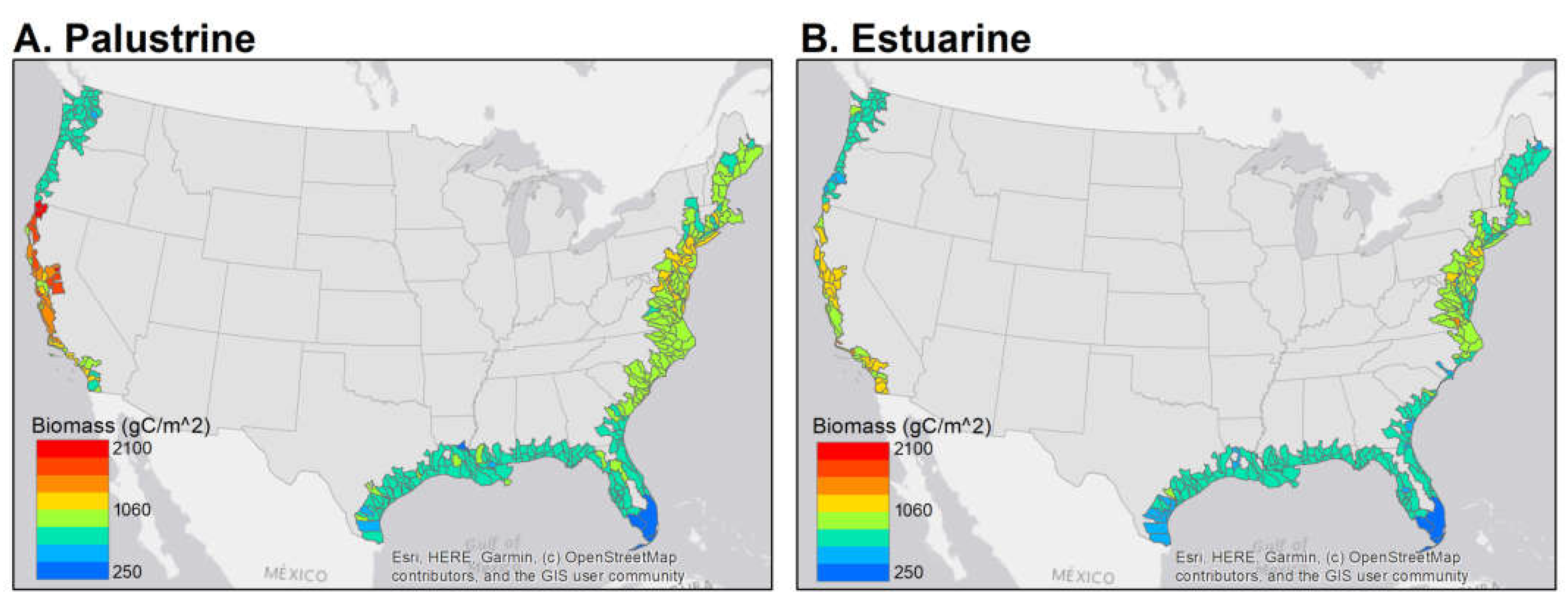
3.1. Spatially Explicit Total Peak Biomass Carbon Stocks

In 2015, the CONUS tidal marsh area was 22,057 km2 (6412 km2 of palustrine and 15,645 km2 of estuarine), containing 18.70 Tg C in plant biomass (5.59 Tg C in palustrine and 13.12 Tg C in estuarine). Peak biomass carbon stocks within each region were similar among palustrine and estuarine herbaceous marsh classes (Figure 2, Table 3). Peak biomass carbon stocks were highest in the California region, with palustrine and estuarine peak means (±SD) of 1441 ± 430 and 1223 ± 288 g C m−2, respectively (Table 3). Four regions contained similar peak biomass carbon stocks, including the Pacific Northwest, Northeast, Mid-Atlantic, and South Atlantic-Gulf regions, with palustrine peak means (±SD) ranging from 838 ± 129 to 1118 ± 206 g C m−2, and estuarine peak means (±SD) ranging from 801 ± 162 to 935 ± 278 g C m−2 (Figure 2, Table 3). The Everglades region had the lowest peak biomass carbon stocks in both the palustrine and estuarine marsh classes, with peak means (±SD) of 309 ± 79 and 283 ± 130 g C m−2, respectively.
Generally, peak biomass carbon stock decreased with decreasing latitude, along the southeast coast. Figure 3 shows the peak total biomass carbon from this study by hydrologic units, as defined by Steeves and Nebert [32]. Within the Mid-Atlantic region, estuarine biomass carbon stocks are lower in South Carolina, compared to other states in the region (Figure 3). In the South Atlantic-Gulf region, biomass carbon stocks in palustrine and estuarine marshes were generally lower in southern Texas than in other areas of the Northern Gulf of Mexico coast and the Atlantic coast.

3.2. Aboveground Turnover Rate and Spatially Explicit Net Primary Production

An extensive literature search was conducted, to estimate tidal herbaceous marsh aboveground biomass turnover rates (AT). Belowground turnover is rarely reported and assumed to be equal to aboveground turnover for modeling purposes. Of the 42 papers reviewed, 18 of these were removed from the dataset because they contained experimental manipulations, such as the use of marsh organs or herbivory boxes [52,53]. The remaining 24 papers reported 4 palustrine and 190 estuarine aboveground turnover values (Supplementary Table S2, Supplementary Figures S1 and S2). In cases where the aboveground turnover rate was calculated using NPP values reported in the literature, the differences in NPP methodology, such as Smalley [54], Weigert and Evans [55], among others, contributed to variability in the AT data (Supplementary Figure S1). Thus, because of the large variability and scarcity of data, we used the median turnover value from the entire dataset, and assumed an aboveground turnover rate of one crop per growing season.
Since NPP was estimated by multiplying peak biomass carbon stock by AT of one crop per year, the NPP and biomass maps have the same spatial pattern. NPP in CONUS tidal marshes totaled 18.70 Tg C y−1 (5.59 Tg C y−1 in palustrine and 13.12 Tg C y−1 in estuarine marshes).

4. Discussion

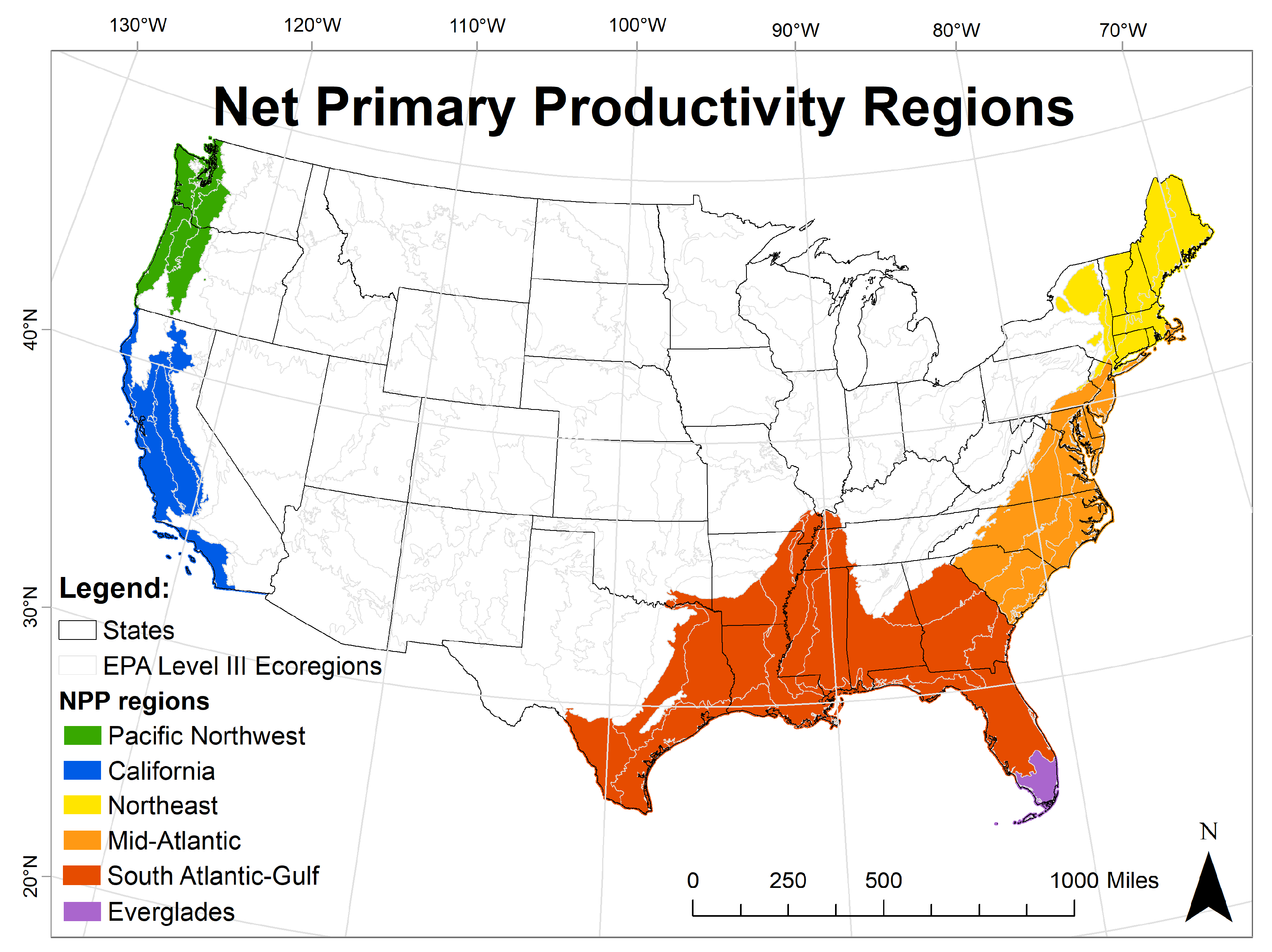
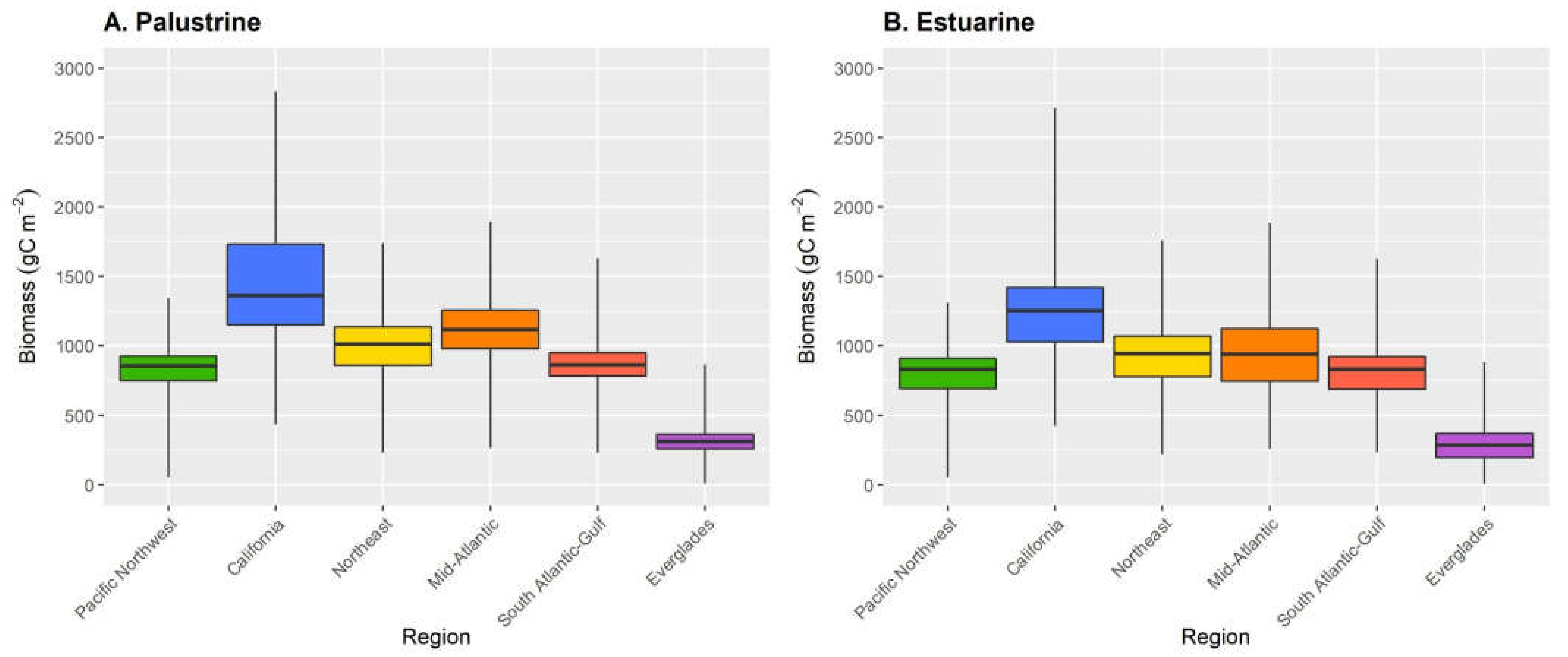
4.1. Regional Trends

The regions in this study were defined based on aggregated level III EPA ecoregions [31] (Table S1), and represent areas with different soils, vegetation, geology, geomorphology, and climate [56]; thus, variation in climate across these regions will influence growing seasons and precipitation, and ultimately biomass values and rates of net primary production. Land use activities can also influence regional patterns of plant growth and productivity [57,58]. Across the six regions, peak biomass carbon stocks were highest in the California region and lowest in the Everglades region, for both palustrine and estuarine herbaceous marsh classes. The spatial patterns in the peak biomass carbon stock maps follow the trends reported in Byrd et al. [22,23]. The high peak biomass carbon stocks in the California region are likely driven by the long growing season [59], due to mild, wet winters and hot summers [60], and the high vegetation density of both palustrine and estuarine marshes, the latter dominated by brackish-marsh and high-marsh plains (e.g., [22,61]). Compared to other regions, where estuarine marshes are comprised of higher-salinity marshes at lower elevations [62], the California region is dominated by brackish marshes, which tend to have higher biomass [8] and NPP [63] compared to saline marshes. In addition, the saline California marshes are dominated by Salicornia pacifica (pickleweed), a perennial herb with woody stems, producing high biomass [64]. In the Everglades, biomass carbon stocks are constrained by the phosphorus-limited environment [65]. Additionally, years of drainage, canal building, and sea-level rise has reduced freshwater flow and increased saltwater intrusion [66]. Prolonged salinity stress in freshwater and brackish Everglades wetlands has led to reduced above- and belowground plant biomass [67]. Frequent disturbances, such as fires, which are common in the Everglades, also have the potential to negatively impact plant production and biomass stocks [68]. Furthermore, peat collapse in the Everglades is linked to sea-level rise, salinity stress, and altered freshwater discharge [67,69], and increased saltwater intrusion is linked with aboveground NPP decreases [70]. In the South Atlantic-Gulf region, biomass carbon stocks in both salinity classes were lowest in southern Texas. Generally, wetland density in southern Texas may be lower due to limited freshwater availability, due to lack of rainfall and high heat [71], leading to hypersaline conditions that are too stressful for vascular plants [72]. Thus, coastal wetlands in southern Texas contain saline and brackish tidal flats that may be dominated by agal mats or completely unvegetated [73].
Regional trends in peak biomass carbon stock are similar between palustrine and estuarine marsh classes. Although increased salinity can diminish plant production in species that are not adapted to saline conditions [74,75], comparative studies of established marsh communities along landscape scale gradients of salinity, illustrate that plant biomass and soil carbon stocks are in fact very similar among different wetland types, and in some cases exhibit greater biomass at higher salinities [63,76].

4.2. Comparisons

Following a literature review of peak aboveground biomass, which included papers from most regions, with the exception of the Pacific Northwest, we confirmed the modeled peak aboveground biomass values were similar, and overlap with, field observations from the literature. In the California region, modeled values ranged from 321 to 2141 g m−2, compared to field values ranging from 300 to 4316 g m−2 [77,78]. In the Northeast region, modeled values ranging from 167 to 1345 g m−2 were similar to field values, ranging from 207 to 1190 g m−2 [79]. In the Mid-Atlantic region, modeled values ranged from 194 to 1432 g m−2, compared to field values ranging from 250 to 3266 g m−2 [80,81]. In the South Atlantic-Gulf region, modeled values ranged from 174 to 1231 g m−2, compared to 181 to 3018 g m−2 reported in the literature [63,82]. In the Everglades region, modeled values of 6 to 675 g m−2 compared to field values ranging from 102 to 880 g m−2 [83]. The overall trend across regions is also similar to that in the literature, with California having higher peak aboveground tidal marsh biomass than the Everglades.
When we compare our NPP map to other available NPP products, such as NASA’s 2015 “MODIS Net Primary Production (NPP)”, with about a 1 km resolution, we observe similar trends, with higher NPP in the Mid-Atlantic and Northeast and lower NPP values in the South Atlantic-Gulf and Everglades regions [84]. However, on the west coast, the NASA NPP map shows slightly lower values in California, when compared to the Pacific Northwest region, unlike our map. Discrepancies in these trends are likely due to the large size of the pixel of the NASA NPP map, which contain mixed land cover classes (e.g., agricultural and forest land covers) that may have very different NPP values per area than herbaceous marshes. When compared to a CONUS tidal wetland map of GPP from Feagin et al. [21], with a 250 m resolution, we see similar patterns on the west coast, where both GPP and NPP are higher in the California region. However, trends in other regions are disparate. Feagin et al. [21] report patterns of higher GPP in the South Atlantic-Gulf and Everglades regions, when compared to northeast and north-central states. For example, in the Everglades, we projected the lowest mean annual rates of NPP, whereas Feagin et al. [21] report the highest mean annual rates of GPP. Feagin et al. [21] rely upon a pixel size that is an order of magnitude greater than our study, which can smooth over and obscure differences at smaller scales, such as differences in land cover classes. Feagin et al. [21] also included scrub/shrub (mangrove) land cover in their assessment, which generate very different biomass and turnover rates than herbaceous marshes, and are highly abundant in the Everglades region. Shrub/scrub vegetation was not included in the original biomass model [22,23] due to limited data, and restricting the model to only herbaceous vegetation greatly improved model performance.
Comparison with other CONUS estimates of carbon fluxes, illustrates the relationship of NPP to net photosynthetic input (GPP) and carbon storage sinks (soil carbon accumulation rate, CAR) in tidal wetlands (Supplementary Figure S3). Every year, a fraction of the NPP carbon flux is stored in the soils, as an autochthonous and typically dominant contribution to annual soil carbon accumulation [85]. For this reason, rates of soil carbon accumulation are usually lower than NPP. Based on our mean CONUS NPP rates, the mean annual rate of carbon fixed in plant biomass was roughly 19% higher than CONUS soil carbon accumulation rates [34]. CONUS GPP from Feagin et al. [21] was roughly 1.9 times higher than our NPP. Because NPP is equal to GPP minus respiration, NPP is always lower than GPP. As expected, our mean NPP values were lower than GPP values for tidal wetlands in all regions, except for in California. NPP values in this region may be artificially inflated, since AT in California may be lower than one (Supplementary Figure S2).

4.3. Limitations

For both salinity classes, very little aboveground turnover rate (AT) data are available for many of the regions, and existing data are highly variable, making precise estimations of regional or marsh class type AT impossible (Supplementary Table S2 and Figure S2). Because AT data was sparse and variable, we assumed AT of one crop per growing season (see Section 2.2). Since NPP is a product of peak biomass carbon stock and AT, having one CONUS-wide value for AT prevented us from seeing different regional patterns in NPP when compared to peak biomass carbon stock. Our estimates of AT were limited by the availability of these labor-intensive datasets (e.g., Coastal Carbon Research Coordination Network (https://serc.si.edu/coastalcarbon, accessed on 10 January 2023) [86]). In the past few decades, there has been a shift towards remote studies, because of the reduced time and cost when compared to field studies. However, future field studies that estimate annual biomass turnover would be beneficial for this assessment and process-based model development (e.g., [87]), especially in regions such as the Pacific Northwest, Everglades, palustrine Northeast, and palustrine California, where data are non-existent (Supplementary Figure S2). Additionally, many biomass and NPP values reported in the literature could not be used to calculate AT, due to missing details regarding sample number and spatial and temporal resolution. We hypothesize that spatial patterns in NPP may differ from peak biomass patterns because of regional differences in turnover rates due to growing season length. Limitations in turnover data representativeness preclude such a refinement of the NPP map today, but may be adjusted in future versions. To date, our NPP map is the only finer-scale estimate of productivity fluxes across CONUS regions, and the least biased data product we can produce at this time.
The methods used to create the biomass carbon map are repeatable for other years. Given the tools provided in this study, the collection of additional field data for independent validation and future AT research, and the generation of new and improved spatial biomass and NPP data products, are possible. Additionally, similar methods could be used to map shrub/scrub and tree wetlands in the future, given that SAVI is a good indication of mangrove and scrub biomass [88,89].
Regarding spatial scale, each pixel of a satellite image may contain a single land cover type (pure), or a mix of land cover types (impure), the larger the pixel is, the more likely it is to be impure. We used the C-CAP land cover data to determine marsh area [37]. As is the case with any remote sensing dataset, this dataset contains some pixels that are impure, but the relatively small pixel size (30 m resolution) limits the effects of pixel impurities, reducing distortion of associated spectral values. In contrast, the GPP map product from Feagin et al. [21], has a 250 m pixel size, and the authors note that many coastal wetlands are linear and smaller than their 250 m pixel size. For this reason, pixel impurity in their map is more common. Pixel impurity can lead to inaccuracies in carbon estimations, through distortion of band values used in a vegetation index, especially those that rely on near-infrared (NIR) reflectance. For example, a pixel that is a mix of vegetated wetland and water—one which strongly reflects NIR and one that strongly absorbs NIR—could have a very different combination of band values than a pure wetland pixel. However, only including pure pixels can result in an underestimation of wetland area. The threshold chosen for area of wetland cover per pixel could have led to the differences in spatial carbon patterns between the estimated NPP and GPP. Given the larger pixel size of MODIS products used by Feagin et al., (2020), the inclusion of forested or productive agricultural lands is more likely to elevate estimated GPP than the inclusion of open water, which typically reduces estimates of GPP. C-CAP pixels, at 30 m resolution, are still inclusive of open water and forested edges, but are less impacted by pixel impurity at larger landscape scales [90]. We note, however, that even the C-CAP land cover map (used in this study) [37] and the National Land Cover Database (NLCD) land cover map [91], define different coverage of herbaceous marshes in CONUS during the same time period, despite having the same spatial resolution. Additionally, different wetland species can have unique and identifiable spectral signatures, but zones of mixed vegetation can have altered spectral peaks, that are hard for models to identify and correctly classify [92].
A potential limitation of this study is the possibility of missed peak SAVI, due to cloud cover or tidal inundation, during the time that the Landsat 8 satellite passed overhead, which is once every 16 days [93]. Tidal inundation has been shown to reduce near-infrared (NIR) reflectance, due to the reduction in aboveground leaf area index (LAI) when vegetation is submerged [94]. NIR is used in the calculation of SAVI and LAI is correlated with SAVI [95].

4.4. Applications

The Intergovernmental Panel on Climate Change (IPCC) provides internationally accepted methods for greenhouse gas (GHG) flux estimations [17,18,19]. In 2013, the IPCC highlighted the importance of including wetlands in national GHG emission estimations in the 2013 Supplement to the 2006 IPCC Guidelines for National Greenhouse Gas Inventories: Wetlands [18]. The IPCC does not recommend specific data or mapping products to be used when determining GHG emissions and removals, allowing each country to use the data that is available to them. GHG flux estimations can vary significantly when different biomass stock data are used. The high-resolution national tidal marsh maps of peak biomass carbon stocks and NPP fluxes created in this study, can be used in a spatially explicit GHG inventory at the Tier 3 level, whereby models of stock gain and loss are modeled at annual increments. Further, the approach used herein is amenable to repeat measurements, and thus annually updatable for model projections of carbon cycling and/or wetland sustainability (e.g., LUCAS, [25]). Additionally, the peak biomass carbon stock and NPP maps can be used to parameterize carbon stock loss and gain for actions relevant to land management (e.g., restoration) [25,96]) or voluntary carbon markets (e.g., [97]).

5. Conclusions

High-resolution (30 m scale) maps of tidal herbaceous marsh total (above- and belowground) peak biomass carbon stocks and NPP, were produced for the first time at the national scale for CONUS. The estimated total peak biomass stocks are 18.70 Tg C, with similar trends in NPP annual flux. Mean values and variability for herbaceous tidal marshes at a 30 m scale, were represented for CONUS as a total peak biomass carbon stock mean and a total NPP mean rate (±standard deviation) of 848 ± 245 g C m−2 [yr−1] (Table 3). Regional variability was slightly greater for palustrine marshes than for estuarine marshes. Total peak biomass carbon stocks were greatest in the California region and lowest in the Everglades region, for both palustrine and estuarine marshes. For all herbaceous tidal wetlands, regardless of salinity class, our CONUS-wide NPP trends were regionally similar to the MODIS-based trends in GPP of Feagin et al. [21], except in the southeast, which is likely due to our exclusion of shrub/shrub wetlands and finer resolution assessment, that likely reduced pixel impurity from mangrove land cover. Our data-model fusion approach to CONUS-wide biomass carbon stock mapping and modeled NPP flux, based on synthesized turnover rates, illustrates the data needs for improving carbon sequestration and GHG emissions inventories in tidal wetlands, whether for national incentives or for voluntary carbon markets, that guide land use policy toward mitigating climate change.

Supplementary Materials

The following supporting information can be downloaded at: https://www.mdpi.com/article/10.3390/rs15061697/s1, Figure S1: Aboveground turnover rate vs. ANPP method, Figure S2: Aboveground turnover vs. dominant vegetation, Figure S3: Regional mean carbon; Table S1: Net primary productivity regions, Table S2: Aboveground turnover from literature review.

Author Contributions

Conceptualization, C.L.S., K.B.B. and L.W.-M.; methodology, V.L.W., C.L.S., K.B.B. and L.W.-M.; validation, V.L.W., C.L.S., K.B.B. and L.W.-M.; formal analysis, V.L.W.; investigation, V.L.W., C.L.S., K.B.B. and L.W.-M.; resources, K.B.B.; data curation, V.L.W., K.B.B. and A.S.R.; writing—original draft preparation, V.L.W., C.L.S. and L.W.-M.; writing—review and editing, V.L.W., C.L.S., K.B.B., L.W.-M., A.S.R. and Z.Z.; visualization, V.L.W., C.L.S. and L.W.-M.; supervision, C.L.S., K.B.B., L.W.-M. and Z.Z.; project administration, C.L.S. and L.W.-M.; funding acquisition, C.L.S. and Z.Z. All authors have read and agreed to the published version of the manuscript.

Funding

This research was funded by the U.S. Geological Survey (USGS) LandCarbon Program, Ecosystems Mission Area, Land Change Science Program, Land Management Research Program, and National Land Imaging Program. A. Rovai was supported by the NASA-JPL Delta-X Mission (https://deltax.jpl.nasa.gov) and by the U.S. Army Engineering, Research and Development Center (ACTIONS project, W912HZ2020070).

Data Availability Statement

Biomass carbon and net primary productivity maps are available in Woltz et al. [51].

Acknowledgments

This work was supported by the U.S. Geological Survey LandCarbon Program, Ecosystem Mission Area, Land Change Science Program, Land Management Research Program and National Land Imaging Program. Significant inputs from the Coastal Carbon Research Coordination Network (CCRCN) and colleagues Lisa Beers and Robert Twilley, allowed regional syntheses. The authors would like to thank Sydney Finn for help in compiling literature values. Any use of trade, firm, or product names is for descriptive purposes only and does not imply endorsement by the U.S. Government.

Conflicts of Interest

The authors declare no conflict of interest.

References

  1. IPCC. Summary for Policymakers. In Climate Change 2021: The Physical Science Basis. Contribution of Working Group I to the Sixth Assessment Report of the Intergovernmental Panel on Climate Change; Masson-Delmotte, V.P., Zhai, A., Pirani, S.L., Connors, C., Péan, S., Berger, N., Caud, Y., Chen, L., Goldfarb, M.I., Gomis, M., Eds.; Cambridge University Press: Cambridge, UK, 2021. [Google Scholar]
  2. Girardin, C.A.; Jenkins, S.; Seddon, N.; Allen, M.; Lewis, S.L.; Wheeler, C.E.; Griscom, B.W.; Malhi, Y. Nature-based solutions can help cool the planet—If we act now. Nature 2021, 593, 191–194. [Google Scholar] [CrossRef]
  3. Mcleod, E.; Chmura, G.L.; Bouillon, S.; Salm, R.; Björk, M.; Duarte, C.M.; Lovelock, C.E.; Schlesinger, W.H.; Silliman, B.R. A blueprint for blue carbon: Toward an improved understanding of the role of vegetated coastal habitats in sequestering CO2. Front. Ecol. Environ. 2011, 9, 552–560. [Google Scholar] [CrossRef] [PubMed] [Green Version]
  4. Chmura, G.L.; Anisfeld, S.C.; Cahoon, D.R.; Lynch, J.C. Global carbon sequestration in tidal, saline wetland soils. Glob. Biogeochem. Cycles 2003, 17, 1111. [Google Scholar] [CrossRef]
  5. Macreadie, P.I.; Costa, M.D.P.; Atwood, T.B.; Friess, D.A.; Kelleway, J.J.; Kennedy, H.; Lovelock, C.E.; Serrano, O.; Duarte, C.M. Blue carbon as a natural climate solution. Nat. Rev. Earth Environ. 2021, 2, 826–839. [Google Scholar] [CrossRef]
  6. Saintilan, N.; Kovalenko, K.E.; Guntenspergen, G.; Rogers, K.; Lynch, J.C.; Cahoon, D.R.; Lovelock, C.E.; Friess, D.A.; Ashe, E.; Krauss, K.W.; et al. Constraints on the adjustment of tidal marshes to accelerating sea level rise. Science 2022, 377, 523–527. [Google Scholar] [CrossRef]
  7. Buffington, K.J.; Dugger, B.D.; Thorne, K.M. Climate-related variation in plant peak biomass and growth phenology across Pacific Northwest tidal marshes. Estuar. Coast. Shelf. Sci. 2018, 202, 212–221. [Google Scholar] [CrossRef]
  8. Buffington, K.J.; Goodman, A.C.; Freeman, C.M.; Thorne, K.M. Testing the interactive effects of flooding and salinity on tidal marsh plant productivity. Aquat. Bot. 2020, 164, 103231. [Google Scholar] [CrossRef]
  9. McKee, K.L.; Mendelssohn, I.A.; Materne, M.D. Acute salt marsh dieback in the Mississippi River deltaic plain: A drought-induced phenomenon? Glob. Ecol. Biogeogr. 2004, 13, 65–73. [Google Scholar] [CrossRef]
  10. Stagg, C.L.; Osland, M.J.; Moon, J.A.; Feher, L.C.; Laurenzano, C.; Lane, T.C.; Jones, W.R.; Hartley, S.B. Extreme Precipitation and Flooding Contribute to Sudden Vegetation Dieback in a Coastal Salt Marsh. Plants 2021, 10, 1841. [Google Scholar] [CrossRef]
  11. Borchert, S.M.; Osland, M.J.; Enwright, N.M.; Griffith, K.T. Coastal wetland adaptation to sea level rise: Quantifying potential for landward migration and coastal squeeze. J. Appl. Ecol. 2018, 55, 2876–2887. [Google Scholar] [CrossRef]
  12. Whigham, D.F.; Baldwin, A.H.; Barendregt, A. Chapter 18: Tidal Freshwater Wetlands. In Coastal Wetlands; Elsevier: Amsterdam, The Netherlands, 2019; pp. 619–640. [Google Scholar]
  13. U.S. Fish and Wildlife Service (FWS). National Wetlands Inventory Website; U.S. Department of the Interior, Fish and Wildlife Service: Washington, DC, USA, 2014.
  14. Couvillion, B.R.; Beck, H.; Schoolmaster, D.; Fischer, M. Land Area Change in Coastal Louisiana 1932 to 2016; Scientific Investigations Map 3381; U.S. Geological Survey: Liston, VA, USA, 2017; p. 16. [Google Scholar] [CrossRef] [Green Version]
  15. Crooks, S.; Sutton-Grier, A.E.; Troxler, T.G.; Herold, N.; Bernal, B.; Schile-Beers, L.; Wirth, T. Coastal wetland management as a contribution to the US National Greenhouse Gas Inventory. Nat. Clim. Chang. 2018, 8, 1109–1112. [Google Scholar] [CrossRef] [PubMed]
  16. U.S. Environmental Protection Agency (EPA). Inventory of US Greenhouse Gas Emissions and Sinks: 1990–2020; EPA 430-R-22-003; US Environmental Protection Agency: Washington, DC, USA, 2022. Available online: https://www.epa.gov/ghgemissions/draft-inventory-us-greenhouse-gas-emissions-and-sinks-1990-2020 (accessed on 1 May 2022).
  17. IPCC. 2006 IPCC Guidelines for National Greenhouse Gas Inventories, Prepared by the National Greenhouse Gas Inventories Programme’s; Eggleston, H.S., Buendia, L., Miwa, K., Ngara, T., Tanabe, K., Eds.; IGES: Hayama, Japan, 2006. [Google Scholar]
  18. IPCC. 2013 Supplement to the 2006 IPCC Guidelines for National Greenhouse Gas Inventories: Wetlands; Hiraishi, T., Krug, T., Tanabe, K., Srivastava, N., Baasansuren, J., Fukuda, M., Troxler, T.G., Eds.; IPCC: Geneva, Switzerland, 2014. [Google Scholar]
  19. IPCC. 2019 Refinement to the 2006 IPCC Guidelines for National Greenhouse Gas Inventories; Calvo Buendia, E., Tanabe, K., Kranjc, A., Baasansuren, J., Fukuda, M., Ngarize, S., Osako, A., Pyrozhenko, Y., Shermanau, P., Federici, S., Eds.; IPCC: Geneva, Switzerland, 2019. [Google Scholar]
  20. Kang, X.; Li, Y.; Wang, J.; Yan, L.; Zhang, X.; Wu, H.; Yan, Z.; Zhang, K.; Hao, Y. Precipitation and temperature regulate the carbon allocation process in alpine wetlands: Quantitative simulation. J. Soils. Sediments 2020, 20, 3300–3315. [Google Scholar] [CrossRef]
  21. Feagin, R.A.; Forbrich, I.; Huff, T.P.; Barr, J.G.; Ruiz-Plancarte, J.; Fuentes, J.D.; Najjar, R.G.; Vargas, R.; Vázquez-Lule, A.; Windham-Myers, L.; et al. Tidal wetland gross primary production across the continental United States, 2000–2019. Global Biogeochem. Cycles 2020, 34, e2019GB006349. [Google Scholar] [CrossRef]
  22. Byrd, K.B.; Ballanti, L.; Thomas, N.; Nguyen, D.; Holmquist, J.R.; Simard, M.; Windham-Myers, L. A remote sensing-based model of tidal marsh aboveground carbon stocks for the conterminous United States. ISPRS J. Photogramm. 2018, 139, 255–271. [Google Scholar] [CrossRef]
  23. Byrd, K.B.; Ballanti, L.; Thomas, N.; Nguyen, D.; Holmquist, J.R.; Simard, M.; Windham-Myers, L. Corrigendum to “A remote sensing-based model of tidal marsh aboveground carbon stocks for the conterminous United States. ISPRS J. Photogramm. 2020, 166, 63–67. [Google Scholar] [CrossRef]
  24. Kurz, W.; Dymond, C.; White, T.; Stinson, G.; Shaw, C.; Rampley, G.; Smyth, C.; Simpson, B.; Neilson, E.; Trofymow, J.; et al. CBM-CFS3: A model of carbon-dynamics in forestry and land-use change implementing IPCC standards. Ecol. Modell. 2009, 220, 480–504. [Google Scholar] [CrossRef]
  25. Sleeter, B.M.; Frid, L.; Rayfield, B.; Daniel, C.; Zhu, Z.; Marvin, D.C. Operational assessment tool for forest carbon dynamics for the United States: A new spatially explicit approach linking the LUCAS and CBM-CFS3 models. Carbon Balance Manag. 2022, 17, 1–26. [Google Scholar] [CrossRef]
  26. Mo, Y.; Kearney, M.S.; Riter, J.A.; Zhao, F.; Tilley, D.R. Assessing biomass of diverse coastal marsh ecosystems using statistical and machine learning models. Int. J. Appl. Earth Obs. Geoinf. 2018, 68, 189–201. [Google Scholar] [CrossRef]
  27. Zhang, Y.; Liang, S. Fusion of multiple gridded biomass datasets for generating a global forest aboveground biomass map. Remote Sens. 2020, 12, 2559. [Google Scholar] [CrossRef]
  28. Sun, S.; Wang, Y.; Song, Z.; Chen, C.; Zhang, Y.; Chen, X.; Chen, W.; Yuan, W.; Wu, X.; Ran, X.; et al. Modelling Aboveground Biomass Carbon Stock of the Bohai Rim Coastal Wetlands by Integrating Remote Sensing, Terrain, and Climate Data. Remote Sens. 2021, 13, 4321. [Google Scholar] [CrossRef]
  29. Breiman, L. Random Forests. Mach. Learn 2001, 45, 5–32. [Google Scholar] [CrossRef] [Green Version]
  30. U.S. Environmental Protection Agency (EPA). National Wetland Condition Assessment 2011: A Collaborative Survey of the Nation’s Wetlands; EPA EPA-843-R-15-005; US Environmental Protection Agency: Washington, DC, USA, 2016.
  31. U.S. Environmental Protection Agency (EPA). Level III Ecoregions of the Continental United States; map scale 1:7,500,000; National Health and Environmental Effects Research Laboratory: Corvallis, OR, USA, 2013. Available online: https://www.epa.gov/eco-research/level-iii-and-iv-ecoregions-continental-united-states (accessed on 2 March 2020).
  32. Steeves, P.; Nebert, D. 1:250,000-Scale Hydrologic Units of the United States; Open-File Report. 94-0236; U.S. Geological Survey: Reston, VA, USA, 1994. Available online: https://water.usgs.gov/lookup/getspatial?huc250k (accessed on 9 January 2021).
  33. Wang, F.; Lu, X.; Sanders, C.J.; Tang, J. Tidal wetland resilience to sea level rise increases their carbon sequestration capacity in United States. Nat. Commun. 2019, 10, 5434. [Google Scholar] [CrossRef] [PubMed] [Green Version]
  34. Herbert, E.R.; Windham-Myers, L.; Kirwan, M. Sea-level rise enhances carbon accumulation in United States tidal wetlands. One Earth 2021, 4, 425–433. [Google Scholar] [CrossRef]
  35. Noe, G.B.; Childers, D.L.; Jones, R.D. Phosphorus biogeochemistry and the impact of phosphorus enrichment: Why is the Everglades so unique? Ecosystems 2001, 4, 603–624. [Google Scholar] [CrossRef]
  36. Richardson, C.J. The everglades: North America’s subtropical wetland. Wetl. Ecol. Manag. 2010, 18, 517–542. [Google Scholar] [CrossRef]
  37. Office for Coastal Management. NOAA’s Coastal Change Analysis Program (C-CAP) 2010 Regional Land Cover Data–Coastal United States. 2022. Available online: https://www.fisheries.noaa.gov/inport/item/48335 (accessed on 19 February 2020).
  38. Holmquist, J.R.; Windham-Myers, L. Relative Tidal Marsh Elevation Maps with Uncertainty for Conterminous USA, 2010; ORNL DAAC: Oak Ridge, TN, USA, 2021. [Google Scholar] [CrossRef]
  39. Kuhn, M.; Wing, J.; Weston, S.; Williams, A.; Keefer, C.; Engelhardt, A.; Cooper, T.; Mayer, Z.; Kenkel, B.; R Core Team; et al. Caret: Classification and Regression Training; R Package Version 6.0-84. 2019. Available online: https://CRAN.R-project.org/package=caret (accessed on 4 November 2021).
  40. R Core Team. R: A Language and Environment for Statistical Computing (3.6.3); R Foundation for Statistical Computing: Vienna, Austria, 2020; Available online: https://www.R-project.org/ (accessed on 4 November 2021).
  41. Huete, A.R. A soil-adjusted vegetation index (SAVI). Remote Sens. Environ. 1988, 25, 295–309. [Google Scholar] [CrossRef]
  42. Gitelson, A.A. Wide dynamic range vegetation index for remote quantification of biophysical characteristics of vegetation. J. Plant Physiol. 2004, 161, 165–173. [Google Scholar] [CrossRef] [Green Version]
  43. Thenkabail, P.S.; Enclona, E.A.; Ashton, M.S.; Van Der Meer, B. Accuracy assessments of hyperspectral waveband performance for vegetation analysis applications. Remote Sens. Environ. 2004, 91, 354–376. [Google Scholar] [CrossRef]
  44. Zhang, M.; Ustin, S.L.; Rejmankova, E.; Sanderson, E.W. Monitoring Pacific coast salt marshes using remote sensing. Ecol. Appl. 1997, 7, 1039–1053. [Google Scholar] [CrossRef]
  45. Byrd, K.B.; Windham-Myers, L.; Leeuw, T.; Downing, B.; Morris, J.T.; Ferner, M.C. Forecasting tidal marsh elevation and habitat change through fusion of Earth observations and a process model. Ecosphere 2016, 7, e01582. [Google Scholar] [CrossRef]
  46. Google Earth Engine. USGS Landsat 8 Surface Reflectance Tier 1. Earth Engine Data Catalog. Available online: https://developers.google.com/earth-engine/datasets/catalog/LANDSAT_LC08_C01_T1_SR (accessed on 31 December 2021).
  47. Falgout, J.T.; Gordon, J. USGS Advanced Research Computing, USGS Yeti Supercomputer; U.S. Geological Survey: Reston, VA, USA, 2021. [Google Scholar] [CrossRef]
  48. U.S. Geological Survey (USGS). Advanced Research Computing. USGS Yeti Supercomputer: U.S. Geological Survey, n.d. Available online: https://www.usgs.gov/advanced-research-computing (accessed on 3 August 2022).
  49. Turner, R.E. Geographic variations in salt marsh macrophyte production: A review. Contrib. Mar. Sci. 1976, 20, 47–68. [Google Scholar]
  50. Edwards, K.R.; Mills, K.P. Aboveground and belowground productivity of spartina alterniflora (smooth cordgrass) in natural and created Louisiana salt marshes. Estuaries 2005, 28, 252–265. [Google Scholar] [CrossRef]
  51. Woltz, V.L.; Stagg, C.L.; Byrd, K.B.; Windham-Myers, L.; Rovai, A.S.; Zhu, Z. Biomass Carbon Stock and Net Primary Productivity in Tidal Herbaceous Wetlands of the Conterminous United States; U.S. Geological Survey: Reston, VA, USA, 2022. [Google Scholar] [CrossRef]
  52. Dame, R.F.; Kenny, P.D. Variability of Spartina alterniflora primary production in the euhaline North Inlet estuary. Mar. Ecol. Prog. Ser. 1986, 32, 71–80. Available online: http://www.jstor.org/stable/24825479 (accessed on 11 February 2020).
  53. Schile, L.M.; Callaway, J.C.; Suding, K.N.; Kelly, N.M. Can community structure track sea-level rise? Stress and competitive controls in tidal wetlands. Ecol. Evol. 2017, 7, 1276–1285. [Google Scholar] [CrossRef]
  54. Smalley, A.E. The Role of Two Invertebrate Populations, Littorina irrorata and Orchelium fificinium, in the Energy Flow of a Salt Marsh Ecosystem. Ph.D. Thesis, University of Georgia, Athens, GA, USA, 1958. [Google Scholar]
  55. Wiegert, R.G.; Evans, F.C. Primary production and the disappearance of dead vegetation on an old field in southeastern Michigan. Ecology 1964, 45, 49–63. [Google Scholar] [CrossRef]
  56. Omernik, J.M.; Griffith, G.E. Ecoregions of the conterminous United States: Evolution of a hierarchical spatial framework. Environ. Manag. 2014, 54, 1249–1266. [Google Scholar] [CrossRef]
  57. Mendelsohn, R. Land Use, Land Use Change, and Forestry: Special Report of the Intergovernmental Panel on Climate Change; Watson, R.T., Noble, I.R., Bolin, B., Ravindranath, N.H., Verardo, D.J., Dokken, D.J., Eds.; Environmental Conservation; Cambridge University Press: Cambridge, UK, 2000; Volume 28, pp. 284–293. [Google Scholar] [CrossRef]
  58. Erb, K.H.; Fetzel, T.; Plutzar, C.; Kastner, T.; Lauk, C.; Mayer, A.; Niedertscheider, M.; Körner, C.; Haberl, H. Biomass turnover time in terrestrial ecosystems halved by land use. Nat. Geosci. 2016, 9, 674–678. [Google Scholar] [CrossRef]
  59. Kukal, M.S.; Irmak, S. US agro-climate in 20th century: Growing degree days, first and last frost, growing season length, and impacts on crop yields. Sci. Rep. 2018, 8, 6977. [Google Scholar] [CrossRef] [PubMed] [Green Version]
  60. U.S. Department of Agriculture (USDA). California Crops Under Climate Change: Impacts and Opportunities for California Agriculture, n.d. Available online: https://www.climatehubs.usda.gov/hubs/california/california-crops-under-climate-change (accessed on 2 February 2023).
  61. Holmquist, J.R.; Windham-Myers, L. A Conterminous USA-Scale Map of Relative Tidal Marsh Elevation. Estuar. Coast 2022, 45, 1596–1614. [Google Scholar] [CrossRef]
  62. Smith, S.M. Vegetation change in salt marshes of Cape Cod National Seashore (Massachusetts, USA) between 1984 and 2013. Wetlands 2015, 35, 127–136. [Google Scholar] [CrossRef]
  63. Stagg, C.L.; Schoolmaster, D.R.; Piazza, S.C.; Snedded, G.; Steyer, G.D.; Fischenich, C.J.; McComas, R.W. A Landscape-scale assessment of above- and belowground primary production in coastal wetlands: Implications for climate change-induced community shifts. Estuaries Coast 2017, 40, 856–879. [Google Scholar] [CrossRef]
  64. Woo, I.; Takekawa, J.Y. Will inundation and salinity levels associated with projected sea level rise reduce the survival, growth, and reproductive capacity of Sarcocornia pacifica (pickleweed)? Aquat. Bot. 2012, 102, 8–14. [Google Scholar] [CrossRef]
  65. Wilson, B.J.; Servais, S.; Charles, S.P.; Mazzei, V.; Gaiser, E.; Kominoski, J.S.; Richards, J.H.; Troxler, T.G. Phosphorus alleviation of salinity stress: Effects of saltwater intrusion on an Everglades freshwater peat marsh. Ecology 2019, 100, e02672. [Google Scholar] [CrossRef]
  66. Lee, D.Y.; Kominoski, J.S.; Kline, M.; Robinson, M.; Roebling, S. Saltwater and nutrient legacies reduce net ecosystem carbon storage despite freshwater restoration: Insights from experimental wetlands. Restor. Ecol. 2021, 30, e13524. [Google Scholar] [CrossRef]
  67. Charles, S.P.; Kominoski, J.S.; Troxler, T.G.; Gaiser, E.E.; Servais, S.; Wilson, B.J.; Davis, S.E.; Sklar, F.H.; Coronado-Molina, C.; Madden, C.J.; et al. Experimental saltwater intrusion drives rapid soil elevation and carbon loss in freshwater and brackish Everglades marshes. Estuar. Coast. 2019, 42, 1868–1881. [Google Scholar] [CrossRef]
  68. Slocum, M.G.; Platt, W.J.; Beckage, B.; Panko, B.; Lushine, J.B. Decoupling natural and anthropogenic fire regimes: A case study in Everglades National Park, Florida. Nat. Areas J. 2007, 27, 41–55. [Google Scholar] [CrossRef]
  69. Wilson, B.J.; Servais, S.; Charles, S.P.; Davis, S.E.; Gaiser, E.E.; Kominoski, J.S.; Richards, J.H.; Troxler, T.G. Declines in plant productivity drive carbon loss from brackish coastal wetland mesocosms exposed to saltwater intrusion. Estuar. Coast 2018, 41, 2147–2158. [Google Scholar] [CrossRef]
  70. Ishtiaq, K.S.; Troxler, T.G.; Lamb-Wotton, L.; Wilson, B.J.; Charles, S.P.; Davis, S.E.; Kominoski, J.S.; Rudnick, D.T.; Sklar, F.H. Modeling net ecosystem carbon balance and loss in coastal wetlands exposed to sea-level rise and saltwater intrusion. Ecol. Appl. 2022, 32, e2702. [Google Scholar] [CrossRef]
  71. Tavakol, A.; Rahmani, V.; Harrington, J. Temporal and spatial variations in the frequency of compound hot, dry, and windy events in the central United States. Sci. Rep. 2020, 10, 1–13. [Google Scholar] [CrossRef]
  72. Withers, K.; Tunnell, J.W.; Judd, F.W. Wind-tidal flats. In The Laguna Madre of Texas and Tamaulipas, 1st ed.; Tunnell, J.W., Judd, F.W., Eds.; Texas A&M University Press: College Town, TX, USA, 2002; pp. 114–126. [Google Scholar]
  73. Osland, M.J.; Grace, J.B.; Guntenspergen, G.R.; Thorne, K.M.; Carr, J.A.; Feher, L.C. Climatic controls on the distribution of foundation plant species in coastal wetlands of the conterminous United States: Knowledge gaps and emerging research needs. Estuar. Coast 2019, 42, 1991–2003. [Google Scholar] [CrossRef]
  74. McKee, K.L.; Mendelssohn, I.A. Response of a freshwater marsh plant community to increased salinity and increased water level. Aquat. Bot. 1989, 34, 301–316. [Google Scholar] [CrossRef]
  75. Willis, J.M.; Hester, M.W. Interactive effects of salinity, flooding, and soil type on Panicum hemitomon. Wetlands 2004, 24, 43–50. [Google Scholar] [CrossRef]
  76. Baustian, M.M.; Stagg, C.L.; Perry, C.L.; Moss, L.C.; Carruthers, T.J.; Allison, M. Relationships between salinity and short-term soil carbon accumulation rates from marsh types across a landscape in the Mississippi River Delta. Wetlands 2017, 37, 313–324. [Google Scholar] [CrossRef] [Green Version]
  77. Callaway, J.C.; Josselyn, M.N. The introduction and spread of smooth cordgrass (Spartina alterniflora) in South San Francisco Bay. Estuaries 1992, 15, 218–226. [Google Scholar] [CrossRef]
  78. Zedler, J.B.; Winfield, T.; Williams, P. Salt marsh productivity with natural and altered tidal circulation. Oecologia 1980, 44, 236–240. [Google Scholar] [CrossRef]
  79. Ruber, E.; Gillis, G.; Montagna, P.A. Production of dominant emergent vegetation and of pool algae on a northern Massachusetts salt marsh. Bull. Torrey Bot. Club 1981, 108, 180–188. [Google Scholar] [CrossRef]
  80. Valiela, I.; Teal, J.M.; Sass, W.J. Production and Dynamics of Salt Marsh Vegetation and the Effects of Experimental Treatment with Sewage Sludge: Biomass, Production and Species Composition. J. Appl. Ecol 1975, 12, 973–981. [Google Scholar] [CrossRef]
  81. Sickels, F.A.; Simpson, R.L. Growth and survival of giant ragweed (Ambrosia trifida L.) in a Delaware River freshwater tidal wetland. Bull. Torrey Bot. Club 1985, 112, 368–375. [Google Scholar] [CrossRef]
  82. Odum, E.P.; Fanning, M.E. Comparison of the productivity of Spartina alterniflora and S. cynosuroides in Georgia coastal marshes. Bull. Ga. Acad. Sci. 1973, 31, 1–12. [Google Scholar]
  83. Daoust, R.J.; Childers, D.L. Ecological effects of low-level phosphorus additions on two plant communities in a neotropical freshwater wetland ecosystem. Oecologia 2004, 141, 672–686. [Google Scholar] [CrossRef]
  84. NASA. MODIS Gross Primary Production (GPP)/Net Primary Production (NPP); MODIS: Moderate Resolution Imaging Spectrometer: Sioux Falls, SD, USA, 2021. Available online: http://modis.gsfc.nasa.gov/data/dataprod/mod17.php (accessed on 19 October 2021).
  85. Breemen, N.; Buurman, P. Biological processes in soils. In Soil Formation, 2nd ed.; Kluwer Academic Publishers: Dordrecht, The Netherlands, 2002; pp. 83–121. [Google Scholar]
  86. Chapman, S.; Villanova University, Villanova, PA, USA. Personal communication, 2021.
  87. Morris, J.T.; Callaway, J.C. Physical and biological regulation of carbon sequestration in tidal marshes. In A Blue Carbon Primer, 1st ed.; Windham-Myers, L., Crooks, S., Troxler, T.G., Eds.; CRC Press: Boca Raton, FL, USA, 2018; pp. 67–79. [Google Scholar]
  88. Utari, D.; Kamal, M.; Sidik, F. Above-ground biomass estimation of mangrove forest using WorldView-2 imagery in Perancak Estuary, Bali. In Proceedings of the IOP Conference Series Earth and Environmental Science, West Java, Indonesia, 17–20 September 2019; IOP Publishing: Bristol, UK, 2020; Volume 500, p. 012011. [Google Scholar]
  89. Bhatti, S.; Ahmad, S.R.; Asif, M. Estimation of aboveground carbon stock using Sentinel-2A data and Random Forest algorithm in scrub forests of the Salt Range, Pakistan. J. For. Res 2022, cpac036. [Google Scholar] [CrossRef]
  90. Ganju, N.K.; Couvillion, B.R.; Defne, Z.; Ackerman, K.V. Development and Application of Landsat-Based Wetland Vegetation Cover and UnVegetated-Vegetated Marsh Ratio (UVVR) for the Conterminous United States. Estuar. Coast 2022, 45, 1861–1878. [Google Scholar] [CrossRef]
  91. MultiResolution Land Characteristics (MRLC) Consortium National Land Cover Database (NLCD). Sioux Falls, SD: U.S. Geological Survey. Available online: http://www.mrlc.gov (accessed on 22 July 2020).
  92. Zeng, J.; Sun, Y.; Cao, P.; Wang, H. A phenology-based vegetation index classification (PVC) algorithm for coastal salt marshes using Landsat 8 images. Int. J. Appl. Earth Obs. Geoinf 2022, 110, 102776. [Google Scholar] [CrossRef]
  93. U.S. Geological Survey (USGS). What are the Acquisition Schedules for the Landsat Satellites? USGS: Science for a Changing World, n.d. Available online: https://www.usgs.gov/faqs/what-are-acquisition-schedules-landsat-satellites#:~:text=Each%20satellite%20makes%20a%20complete,scene%20area%20on%20the%20globe (accessed on 12 December 2022).
  94. Kearney, M.S.; Stutzer, D.; Turpie, K.; Stevenson, J.C. The effects of tidal inundation on the reflectance characteristics of coastal marsh vegetation. J. Coast Res. 2009, 25, 1177–1186. [Google Scholar] [CrossRef]
  95. Ray, S.S.; Das, G.; Singh, J.P.; Panigrahy, S. Evaluation of hyperspectral indices for LAI estimation and discrimination of potato crop under different irrigation treatments. Int. J. Remote Sens. 2007, 27, 5373–5387. [Google Scholar] [CrossRef]
  96. Sleeter, R.; Sleeter, B.M.; Williams, B.; Hogan, D.; Hawbaker, T.; Zhu, Z. A carbon balance model for the great dismal swamp ecosystem. Carbon Balance Manag. 2017, 12, 1–20. [Google Scholar] [CrossRef] [PubMed]
  97. Sapkota, Y.; White, J.R. Carbon offset market methodologies applicable for coastal wetland restoration and conservation in the United States: A review. Sci. Total Environ. 2020, 701, 1–9. [Google Scholar] [CrossRef] [PubMed]
Figure 1. Regions used to study wetland biomass and net primary productivity (NPP).
Remotesensing 15 01697 g001
Figure 2. Peak total (above- and belowground) biomass carbon in (A) palustrine and (B) estuarine herbaceous tidal marshes by region. Box plot boundaries closest to zero represent the 25th percentile, the line within the boxes indicates the median, and boundaries farthest from zero represent the 75th percentile.
Remotesensing 15 01697 g002
Figure 3. Peak total (above- and belowground) biomass carbon in palustrine and estuarine herbaceous wetlands by hydrologic unit.
Remotesensing 15 01697 g003
Table 1. The seven model predictors used in the random forest biomass model.
Soil adjusted vegetative index (SAVI):
1: SAVI = ((NIR − R)/(NIR + R + 0.5)) × 1.5
Wide dynamic range vegetation index (WDRVI):
2: WDRVI = (0.5 × NIR − R)/(0.5 × NIR + R)
Two-band vegetation indices (TBVI):
3: TBVIRG = (R − G)/(R + G)
4: TBVIGB = (G − B)/(G + B)
5: TBVISR = (Swir2 − R)/(Swir2 + R)
6: TBVISN = (Swir2 − NIR)/(Swir2 + NIR)
Region
7: Wetland NPP region *
Where NIR, R, G, B, and Swir2 are the near-infrared, red, green, blue, and shortwave infrared 2 bands. * Each region was assigned one predictor class, except for the California region which was split into two classes based on salinity.
Table 2. Variable importance from the Landsat based random forest biomass model.
VariableImportance Score
SAVI100
nd_swir2_r95.59
Everglades91.98
San Francisco Bay-freshwater80.29
WDRVI575.17
nd_g_b72.45
nd_swir2_nir69.2
nd_r_g49.75
San Francisco Bay-brackish and saltwater38.7
Puget Sound13.17
Louisiana0.57
Chesapeake0
Table 3. Total tidal marsh area and total (above- and belowground) peak biomass carbon stock for each marsh class, within each region.
Marsh ClassRegionArea (km2)Mean Total Carbon ±SD (g C m−2)
PalustrinePacific Northwest217838 ± 129
California1331441 ± 430
Northeast58998 ± 205
Mid-Atlantic7241118 ± 206
South Atlantic-Gulf4854868 ± 123
Everglades426309 ± 79
EstuarinePacific Northwest86801 ± 162
California3431223 ± 288
Northeast253923 ± 217
Mid-Atlantic4266935 ± 278
South Atlantic-Gulf10,279806 ± 172
Everglades419283 ± 130
Disclaimer/Publisher’s Note: The statements, opinions and data contained in all publications are solely those of the individual author(s) and contributor(s) and not of MDPI and/or the editor(s). MDPI and/or the editor(s) disclaim responsibility for any injury to people or property resulting from any ideas, methods, instructions or products referred to in the content.

