Article

A Performance Analysis of Soil Dielectric Models over Organic Soils in Alaska for Passive Microwave Remote Sensing of Soil Moisture

1
Department of Engineering Systems and Environment, University of Virginia, Charlottesville, VA 22904, USA
2
NASA Jet Propulsion Laboratory, California Institute of Technology, Pasadena, CA 91109, USA
3
NASA Goddard Space Flight Center, Greenbelt, MD 20771, USA
*
Author to whom correspondence should be addressed.
Remote Sens. 2023, 15(6), 1658; https://doi.org/10.3390/rs15061658
Submission received: 28 January 2023 / Revised: 16 March 2023 / Accepted: 17 March 2023 / Published: 19 March 2023
(This article belongs to the Special Issue Microwave Remote Sensing of Soil Moisture)

Abstract

:
Passive microwave remote sensing of soil moisture (SM) requires a physically based dielectric model that quantitatively converts the volumetric SM into the soil bulk dielectric constant. Mironov 2009 is the dielectric model used in the operational SM retrieval algorithms of the NASA Soil Moisture Active Passive (SMAP) and the ESA Soil Moisture and Ocean Salinity (SMOS) missions. However, Mironov 2009 suffers a challenge in deriving SM over organic soils, as it does not account for the impact of soil organic matter (SOM) on the soil bulk dielectric constant. To this end, we presented a comparative performance analysis of nine advanced soil dielectric models over organic soil in Alaska, four of which incorporate SOM. In the framework of the SMAP single-channel algorithm at vertical polarization (SCA-V), SM retrievals from different dielectric models were derived using an iterative optimization scheme. The skills of the different dielectric models over organic soils were reflected by the performance of their respective SM retrievals, which was measured by four conventional statistical metrics, calculated by comparing satellite-based SM time series with in-situ benchmarks. Overall, SM retrievals of organic-soil-based dielectric models tended to overestimate, while those from mineral-soil-based models displayed dry biases. All the models showed comparable values of unbiased root-mean-square error (ubRMSE) and Pearson Correlation (R), but Mironov 2019 exhibited a slight but consistent edge over the others. An integrated consideration of the model inputs, the physical basis, and the validated accuracy indicated that the separate use of Mironov 2009 and Mironov 2019 in the SMAP SCA-V for mineral soils (SOM < 15%) and organic soils (SOM 15%) would be the preferred option.

1. Introduction

Passive microwave remote sensing is considered the most suitable tool for mapping spatial soil wetness, owing to the negligible atmospheric influence and less interference from canopy and surface roughness [1,2]. The remarkable performance of soil moisture (SM) retrievals from spaceborne L-band radiometers (i.e., soil moisture and ocean salinity (SMOS) [3] and soil moisture active passive (SMAP) [4]) has been substantiated by a number of validation studies [5,6,7,8,9]. The mechanism that physically bridges the surface emission at microwave bands and surface SM is based on the contrasting difference between the dielectric constants of liquid water (~80) and dry soil (~4) [10]. The dielectric model that quantitatively links the SM with the bulk dielectric constant of the soil–water–air system is therefore critical in the retrieval algorithms of SMOS and SMAP.
Recently, numerous dielectric models were developed and applied for both spaceborne microwave radiometers and in-situ electromagnetic sensors [11]. An ideal dielectric model is envisioned, to accurately account for the dielectric response of wet soils as a function of all the relevant factors, including soil compaction, soil composition, the fraction of bound and free water, salinity, soil temperature, soil particle size distribution, and observation frequency, etc. [12]. However, the practical dielectric models are often established on a limited set of soil properties and are unable to approximate proper dielectric constants for all the surface conditions. Previous studies found that applying mineral-soil-based dielectric models over organic soils could lead to a substantial underestimation of SM [11]. [13] revealed a significant drop in SMAP retrieval quality in regions with soil organic carbon (SOC) exceeding 8.72%. Given that Mironov 2009 [14], currently used in the SMOS and SMAP operation algorithms, was developed exclusively on samples of mineral soils, an update on the dielectric model that incorporates the effect of soil organic matter (SOM) is pressingly required for areas with organic-rich soils.
The influence of SOM on the bulk dielectric constant of the soil–water system is often summarized in two aspects. First, organic substrates have larger specific surface areas than minerals, indicating that organic soil has a higher fraction of bound water relative to mineral soil, when they contain the same amount of water [11,15,16]. As such, at the same moisture, the dielectric constant of organic soil tends to be lower than that of mineral soil, as the dielectric constant of bound water is much smaller than that of free water. Second, organic soil is often marked by a larger porosity than mineral soil, due to its complex structure [11,15,16,17]. Based on these principles, several organic-soil-based dielectric models have been developed in recent years.
Although model developers pointed out the potential applicability of their models in the retrieval of SM, assessment of the efficacy of these newly developed organic-soil-based dielectric models in the derivation of passive microwave remote sensing of SM has not been widely carried out. In light of these considerations, nine advanced dielectric mixing models were selected and tested in the context of the SMAP single-channel algorithm at vertical polarization (SCA-V) [18]. This study has two major objectives: (1) present the differences between the available mineral- and organic-soil-based models, in describing the complex dielectric behaviors of wet soils under various SOM conditions; and (2) evaluate their performance in organic-rich soils. The latter was achieved by comparing the SCA-V SM retrievals from different models against in-situ measurements scattered over Alaska, where the soils are identified with a noticeably higher SOM (~25%) relative to the global average level (Figure A1). The dielectric models considered here have been classified as mineral-soil-based dielectric models, including Wang 1980 [19], the semi-empirical Dobson 1985 modified by Peplinski 1995 [12,20] (hereafter Dobson 1985), the prevalent Mironov 2009 [14], Mironov 2012 [21], and Park 2017 [22], and organic-soil-based dielectric models, including the natural log fitting model in [11] (hereafter Bircher 2016), Mironov 2019 [23], Park 2019 [16], and Park 2021 [24].
As introduced earlier, five mineral-soil-based dielectric models were selected for a comprehensive survey of diverse models in the framework of the SMAP SCA-V algorithm over organic-rich soils. Two of them, Mironov 2013 and Park 2017, have not been widely examined under the SMOS and SMAP schemes [22,25]. In contrast, the other three classic models have been extensively assessed in wide domains covered by mineral soils [26,27,28]. However, their performances over regions with high SOM proportions have not been well-studied and compared with those of dedicated organic-soil-based models. In addition to water volume, mineral-soil-based models primarily focus on the influence of soil texture, commonly characterized by sand, clay, and silt. Yet, organic-soil-based models place a greater emphasis on the SOM effect. Mironov 2019, for example, describes all parameters as functions of SOM rather than the clay percentage used in Mironov 2009 [23]. Therefore, incorporating more mineral- and organic-soil-based models may also help to construct an impression of their systematic differences when describing the dielectric behaviors of organic soils.
The paper is organized as follows. In Section 2, all the data sets and preprocessing steps are presented. Next are the workflow of in-situ measurements screening and the partial SMAP SCA-V retrieval process used to derive the SM from the identical observations and different models (Section 3). The results of the synthetic experiments, validation consequences over Alaska, and a detailed discussion are subsequently displayed in Section 4. Finally, the conclusions are followed by a brief summary presented in Section 5.

2. Data

2.1. SMAP L2 Radiometer Half-Orbit 36 km EASE-Grid Soil Moisture, Version 8

Launched on 31 January 2015, the SMAP mission was designed to map high-resolution SM and freeze/thaw state by combining the attributes of L-band radar and radiometer. However, the SMAP SM products presently rely on radiometer observations alone, due to an unexpected malfunction of the SMAP radar in July 2015. With an average revisit frequency of two to three days, the SMAP sensors cross the Equator at the local solar times of 6 a.m. and 6 p.m.
SMAP L2 Radiometer Half-Orbit 36 km EASE-Grid Soil Moisture, Version 8 (SMAP V8) [29] was adopted in this study. Here, we only used the descending (6 a.m.) SM retrievals derived using the SCA-V algorithm. A series of masking procedures were utilized to avoid the application of SM retrievals of low accuracy and high uncertainty. Specifically, only the retrievals flagged as the “recommended quality” were retained and employed in the later analysis. Given Alaska, the focused region of this study, is located in the high-latitude portion with a long-term frozen duration, we only considered those qualified SM retrievals within the time intervals from June to August, between 2015 and 2021.
One noticeable improvement in SMAP V8 (relative to the older version) is the update and extension of gridded soil parameters, ranging from SOC, silt and sand fractions to bulk density. These newly added soil attributes originate from the SoilGrid 250 m [30] and replace the earlier patched version composed of the National Soil Data Canada (NSDC), the State Soil Geographic Database (STATSGO), the Australia Soil Resources Information System (ASRIS), and the Harmonized World Soil Database (HWSD) [31]. Since these soil attributes are often necessary inputs for dielectric models of soil, they were also extracted from the SMAP V8.

2.2. In-Situ Soil Moisture Measurements

Ground-based SM measurements over Alaska were employed as benchmarks to assess the skills of the diverse dielectric mixing models. Historical files of soil water content observed by in-situ sensors were first downloaded from the Natural Resources Conservation Service (NRCS), the National Water and Climate Center (NWCC) homepage (https://www.nrcs.usda.gov/wps/portal/wcc/home (accessed on 7 April 2022)). At present, there are more than 40 operating stations from the Snow Telemetry (SNOTEL) [32] and Soil Climate and Analysis Network (SCAN) [33]. These stations are able to monitor the sub-daily variations of SM and many other climatic variables in near real time.
However, some typical errors [34] of in-situ SM readings, such as breaks and plateaus, were found before their application. As a response, the other authoritative data source of in-situ SM, the International Soil Moisture Network (ISMN) [35,36], was also considered, aiming at incorporating its flag information. Given the limited stations in Alaska, it is expected that SM data from the above two sources (NWCC and ISMN) are mostly from the same set of stations. Additionally, for the same station, the observed SM time series from the NWCC and ISMN should be identical, as the ISMN only gathers data and harmonizes them in units and time steps, without extra data processing. Given the frequently abnormal SM readings (even after adopting the quality flag) and the necessity of checking the consistency of SM measurements from two different sources, several rigorous pre-checking procedures were applied (as described in Section 3.1) to filter out those suspicious observations where possible in advance.

3. Methodology

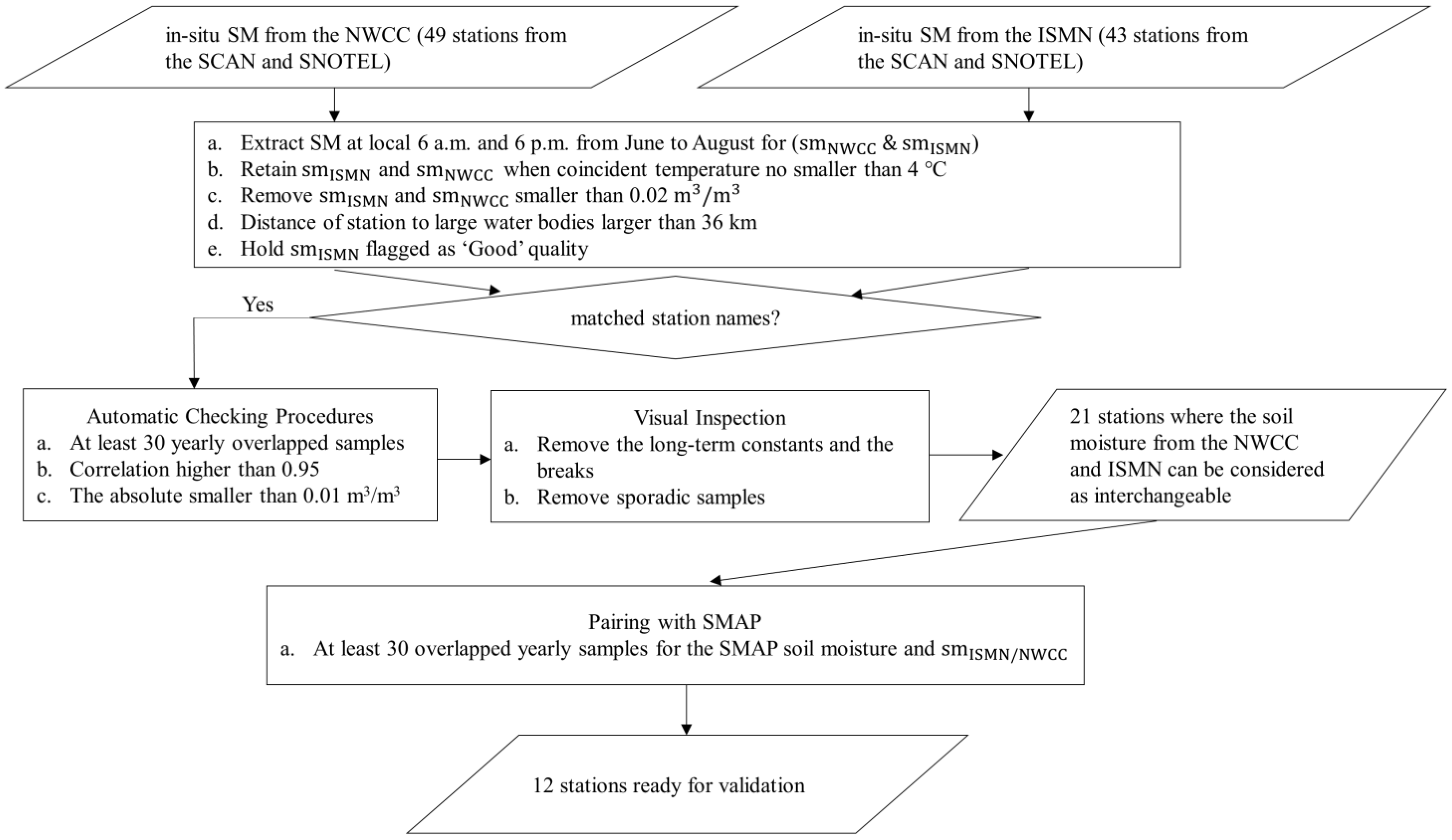
3.1. Preliminary Examination of In-Situ Measurements

The quality of in-situ SM data is of great importance, as these ground measurements are generally seen as the benchmark for evaluating remotely sensed and/or modeled SM data sets [5,6,7]. However, monitoring SM dynamics over high-latitude regions is still challenging, due to the long-term frozen periods and harsh environments. Such difficulties have been reflected by the flat limbs and breaks frequently occurring in the SM time series from the Alaskan stations. Given those, a careful examination of in-situ SM measurements is necessary.
The general workflow of the preliminary examination steps is delineated in Figure 1. Specifically, the in-situ SM data measured at the local time of 6 a.m. and 6 p.m. (temporally align with the SMAP overpass time) were first extracted from the NWCC and ISMN stations. SM measurements with the corresponding land surface temperature below 4 °C were excluded, as [6] demonstrates that some sensors begin to behave abnormally under this temperature. Meanwhile, the utilization of such a threshold would also be helpful to filter out those SM measurements likely obtained during a period of active thawing and re-freezing, where SM fluctuations are excessively unstable (e.g., Figure 3c in [34]). Additionally, stations with a distance shorter than 36 km to large water bodies or oceans were also masked, as the SMAP SM over those regions is likely influenced by water contamination. The flag information from the ISMN was also incorporated to filter the in-situ data of low quality.
The matched SM data of the overlapped stations from the NWCC and ISMN are anticipated, and this greater consistency further enhances the reliability of these benchmarks. Therefore, an automatic consistency checking procedure, constrained by three requirements, was applied. Since breaks and plateaus still appeared on the SM time series after consistency checking, a manual visual inspection was then performed to screen these suspicious measurements. After those, there were 21 qualified stations left, and we assumed that their SM data from the NWCC and ISMN are interchangeable. Furthermore, pairing with the SMAP observations removed nine stations, and the remaining 12 stations (Figure S1) were used in the later validation steps.

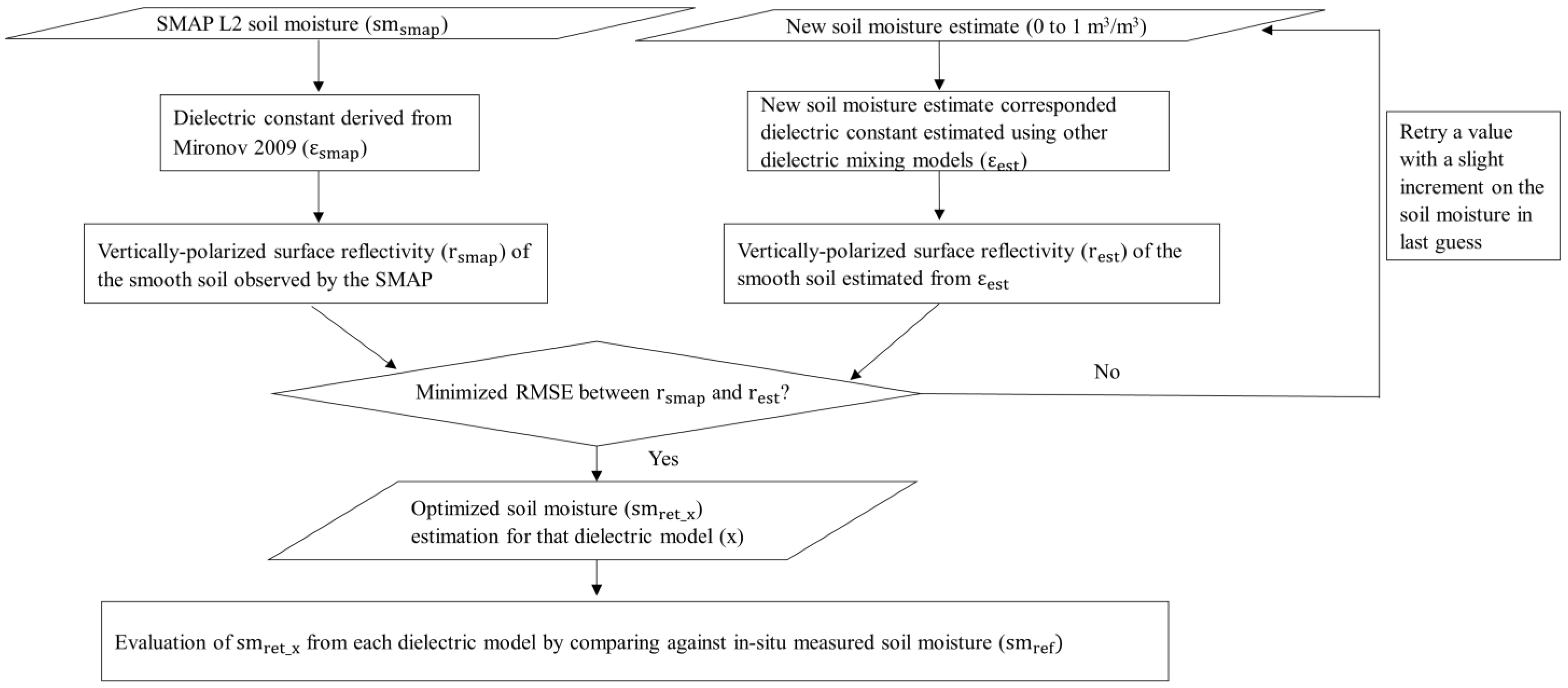
3.2. Derivation of Soil Moisture from Various Dielectric Models

In the SCA-V algorithm, the SMAP SM value is determined when there is a minimized difference between the simulated and the observed reflectivity ( r s m a p ) (reflectivity = 1 − emissivity) of smooth soil. At each temporal step, the value of r s m a p over a pixel is fixed, as the SMAP SCA algorithm determines the radiative contribution from the canopy layer and the impact of surface roughness before subtracting them from SMAP observed surface brightness temperature ( T B ). Hence, the influence of adopting different dielectric constant models on SM retrievals can be examined using the iterative feedback-loop procedure, to minimize the difference between the simulated reflectivity ( r e s t ) and r s m a p , and without the need to construct the whole process from SM to T B , in consideration of simplicity.
However, r s m a p is an intermediate product and unavailable in the original SMAP data set. Given this, the values of r s m a p were first estimated leveraging SMAP SM and Mironov 2009. With these benchmarks, the SM retrievals of other dielectric models were then acquired based on the optimization flow described in Figure 2. Notably, the SM retrieval at a given time point is reproducible when the identical r s m a p and model are used.

3.3. Performance Metrics

The capability of the remote sensing SM data set has been described by four conventional metrics, which are bias, root-mean-square error (RMSE), unbiased root-mean-square error (ubRMSE), and the Pearson Correlation (R) [37]. These metrics could effectively reflect the discrepancies in terms of magnitude, as well as the links of the temporal evolutions between the SM estimations and the ground truth. The formulas used to compute these metrics are shown in Equations (1)–(4), where E […] represents the arithmetic mean; and σ o p t and σ r e f denote the standard deviations of SM retrievals of the respective dielectric models and in-situ measured SM.
b i a s = E s m r e t E [ s m r e f ]
R M S E = E [ ( s m r e t s m r e f ) 2 ]
u b R M S E = R M S E 2 b i a s 2
R = E [ ( s m r e t E [ s m r e t ] ) ( s m r e f E [ s m r e f ] ) ] σ r e t σ r e f

4. Results and Discussion

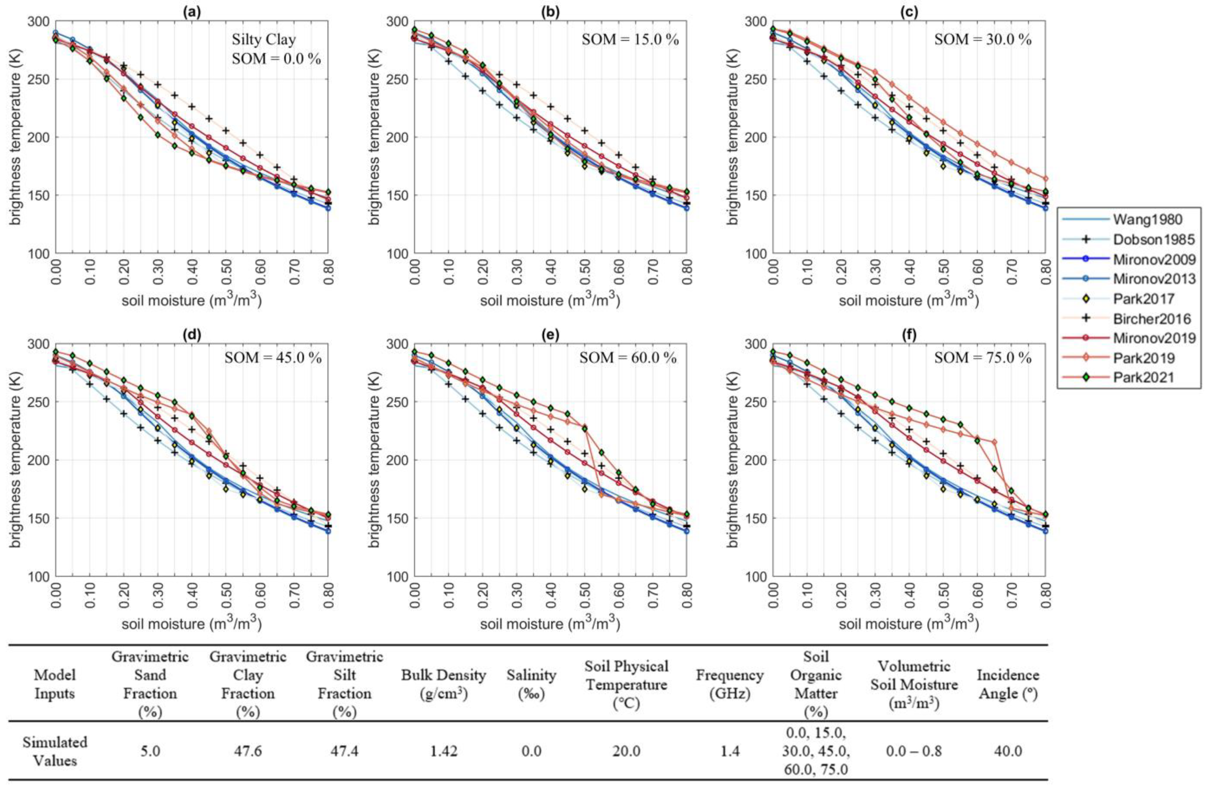
4.1. Simulated Brightness Temperature of Smooth Soil through Synthetic Experiments

Synthetic experiments have the capability to afford complete dielectric responses to a whole SM range, by artificially controlling all the inputs required for the dielectric models (Table 1). With the SOM increasing from 0% to 75% at a step of 15%, the differences between the dielectric constants estimated by mineral- and organic-soil-based dielectric models were explored. These various dielectric responses were further transferred to their corresponding thermal radiations of smooth soils, represented by the vertically polarized T B .
Figure 3 presents the T B curves derived using different dielectric models, across the range of SM from 0 to 0.8 m3/m3. Generally, the T B values estimated using organic-soil-based models are greater than those derived using the mineral-soil-based models, particularly when SOM exceeds 15% and the SM is higher than 0.1 m3/m3. In other words, the SM retrievals from organic-soil-based models tend to be wetter than the SM retrievals from mineral-soil-based models (e.g., Mironov 2009) given the same surface reflectivity (or T B ) of bare, smooth soil. The discrepancies between the simulated T B magnitudes from mineral- and organic-soil-based models further grow with the increase of SOM (Figure 3). However, it should be noted that the estimated dielectric constants and their subsequent T B values from mineral-soil-based models do not vary with SOM. The higher SM estimations of organic-soil-based models relative to mineral-soil-based models could be attributed to the fact that these organic-soil-based models assume a higher volumetric proportion of bound water [11,15,16]. When the SOM is at 15% (and below), the simulated T B curves from all the considered models are clustered together, bounded by Dobson 1985 and Bircher 2016 (Figure 3b). Therefore, the SOM of 15% might be treated as an appropriate demarcation point for the separate use of mineral- and organic-soil-based dielectric models over mineral soils and organic soils.
Moreover, similar features of the T B curves of those considered dielectric models have been observed when a sandy sample is tested (Figure S2). Such a stable-magnitude discrepancy between the red curves (organic models) and the blue curves (mineral models) under contrasting textures (sandy and clay soils) can be attributed to the insensitivity of the organic-soil-based dielectric models to soil texture. For example, Mironov 2019 only accounts for the effects of soil moisture, SOM, and soil temperature on the dielectric permittivity of organic soils (Table 1). Although Park 2019 and Park 2021 incorporate both textural and SOM information, the differences in their estimated T B values from sandy and clay samples seem insignificant under the same SOM level (Figure 3 and Figure S2).
Compared to Mironov 2019, the influence of organic content on the simulated T B magnitude seem more pronounced for Park 2019 and Park 2021. When the SOM increases from 0% to 75% and the SM values are smaller than 0.5 m3/m3, the T B curve of Park 2021 jumps from the bottom to the top line, with a varying amplitude on the order of tens of Kelvins (Figure 3). In contrast, as a response to the growing SOM, the estimations from Mironov 2019 slowly move upward, approaching the T B curve of Bircher 2016. According to Figure 3e,f, there is a rapidly dropping segment on the T B curve of Park 2019. Such abnormal dielectric behavior can be attributed to the improper formulas used to calculate the wilting point and porosity, with a detailed explanation in Section 4.4.

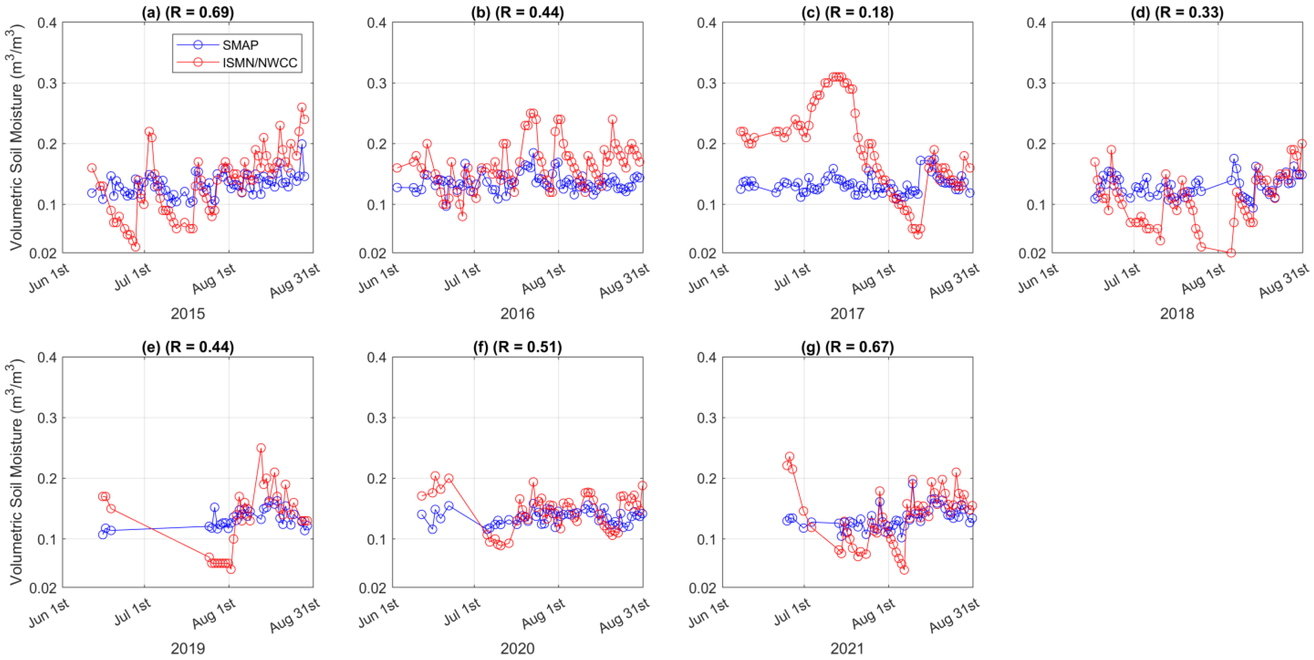
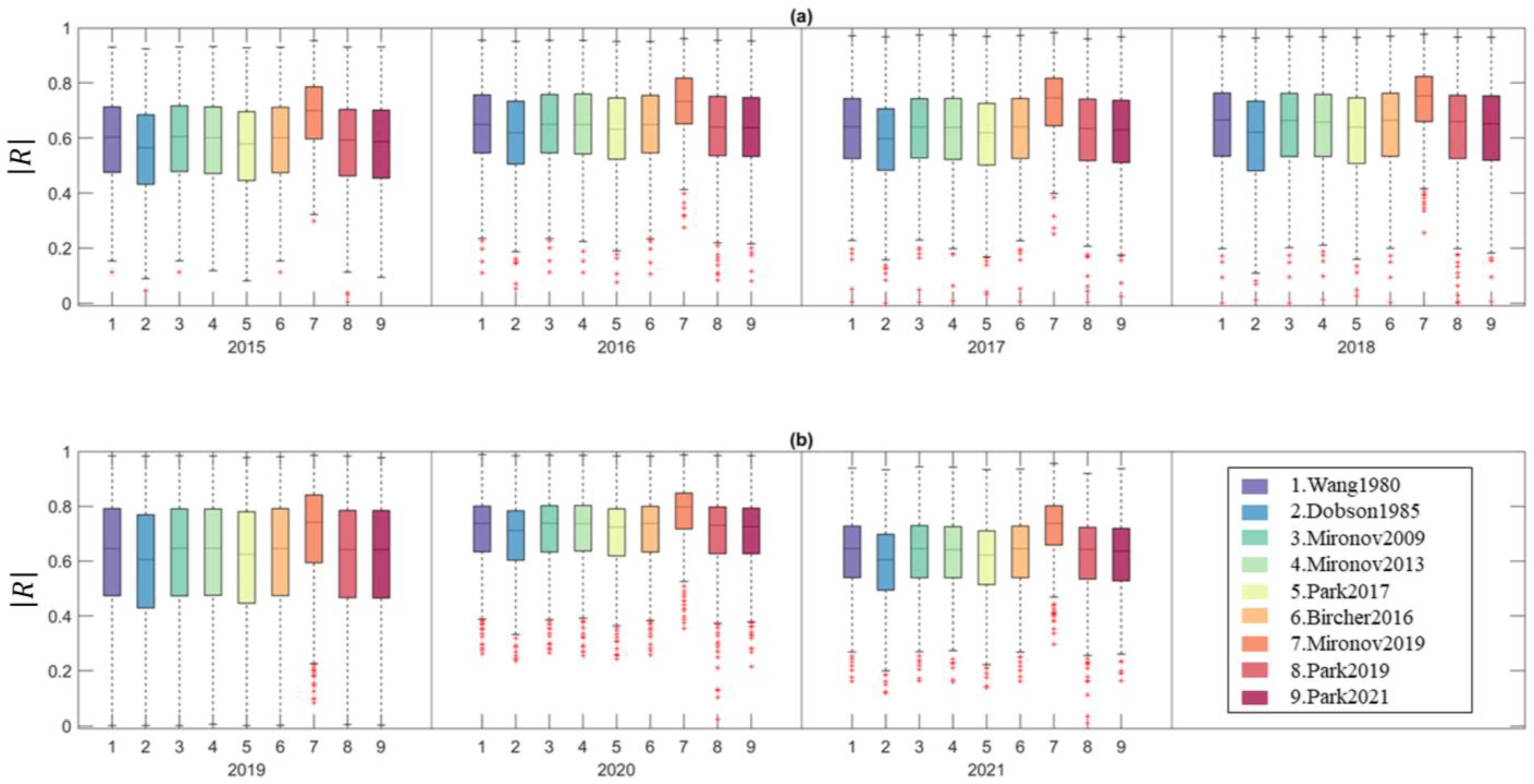
4.2. Evaluation of Dielectric Models over In-Situ Sites in Alaska

Here, SM measurements from 12 sites served as benchmarks to evaluate the skills of the multiple dielectric models in the setting of SMAP observations and the SCA-V algorithm. Before inter-comparison, it was found that the assessment metrics of the satellite-based SM retrievals over the same pixel could vary a lot in different years. Using the time series in Monument Creek as an instance (Figure 4), the R values ranged from 0.18 (2017) to 0.69 (2015). Hence, the obtained metrics (Table 2, Table 3 and Table 4) averaged over multiple years of each station might be underrated, as they may have been compromised by abnormal behavior in one year. Additionally, the amplitudes and frequencies of in-situ SM variations are often more pronounced relative to the SM retrievals, as the latter reflects the changes over a coarse spatial extent (Figure 4). SM variations at local scales often cannot be captured by the 36 km-scale SM retrievals, due to the omission of spatial variability within the footprint-scale area. As noted by [39], spatial mismatching between satellite SM retrievals and point-scale in-situ measurements could adversely impact the perceived accuracy of SMAP observations.
Assessment metrics of the SM retrievals derived using identical r s m a p values and different dielectric models were computed by their temporally paired in-situ measurements. According to Table 2, the SM estimates from mineral-soil-based models tend to underestimate, while the organic-soil-based models generally exhibit wet biases compared to the ground recordings. In terms of both ubRMSE and R (Table 3 and Table 4), all the models show comparable accuracy levels, similar to the previous results in [27], whereas Mironov 2019 displays a slight but consistent edge over the other models. Compared to the other dielectric models, the modest improvement in R of Mironov 2019 was likely due to its simultaneous consideration of bulk density and SOM effects [23].
The other aspect that we attempted to evaluate for the predictive power of various dielectric models was checking the correlations between the SM retrievals of different models and SMAP observed vertically polarized T B . If the higher absolute R values between the time series of SM and SMAP vertically polarized T B are assumed as a criterion that reflects the better skill of a dielectric mixing model, Mironov 2019 presents an overwhelming superiority over the other models in the 765 Alaskan pixels (Figure 5). Table S2 displays that in-situ measured SM usually has a lower correlation with SMAP vertically polarized T B relative to the correlations between satellite-based SM retrievals and SMAP T B . However, it should be noted that such correlation-based results were inconclusive and functioned as a reference only, since the impacts of vegetation disturbance and surface roughness were entirely ignored.

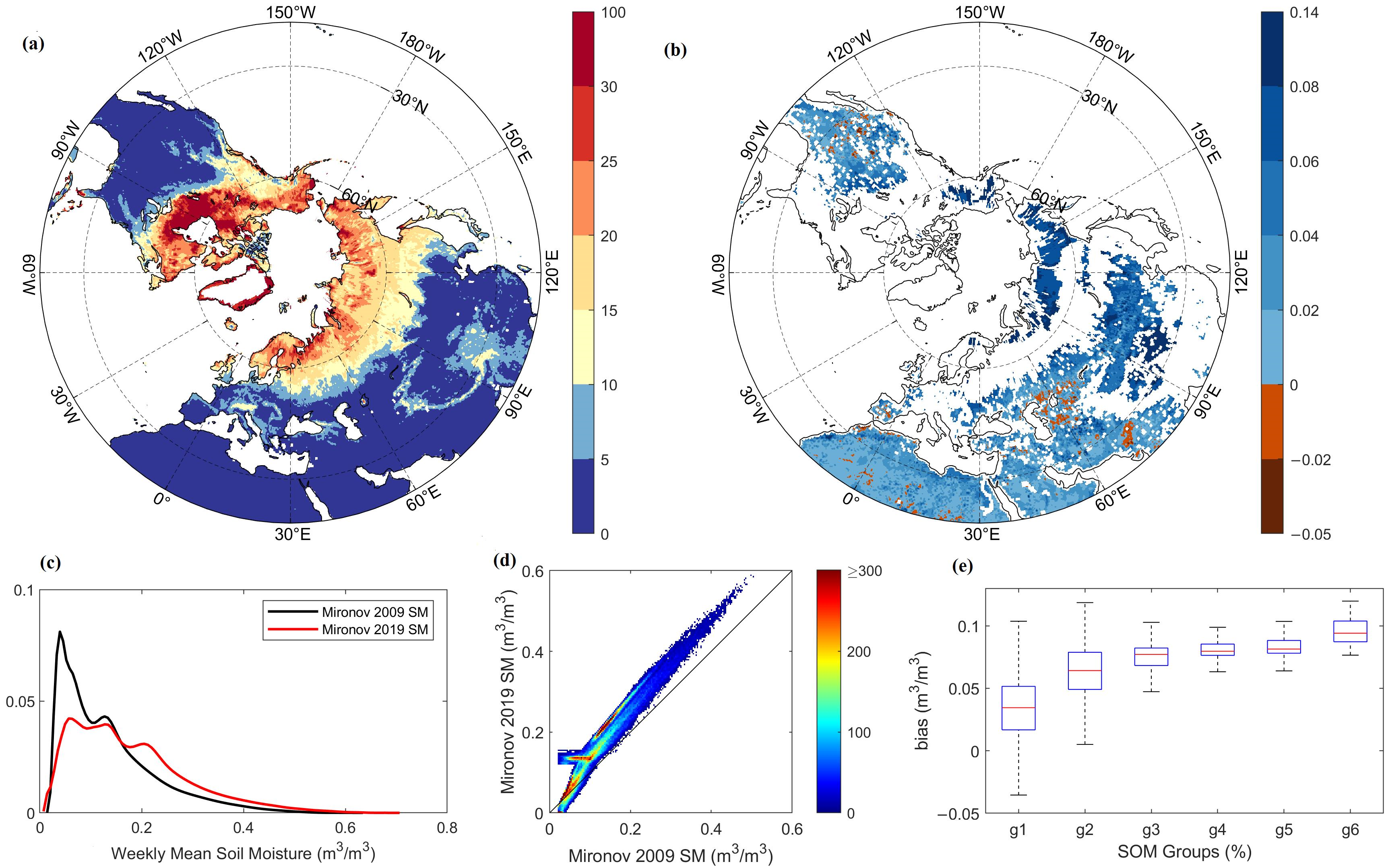
4.3. A Global Intercomparison between Mironov 2009 and Mironov 2019

Mironov 2009 and Mironov 2019 were selected as the representatives for mineral- and organic-soil-based dielectric models and were then compared with each other at the global scale using one-week SMAP observations from 2 July 2018 to 8 July 2018. The one-week SM retrievals of Mironov 2009 and Mironov 2019 were analyzed over more regions with abundant SOM and were also used to acquire performance clues for applying Mironov 2019 to mineral soils.
According to Figure 6a,b, satellite-based SM data are usually unavailable in many areas characterized by organic-rich soils, likely owing to dense boreal forests, steep surface roughness, as well as permanently frozen soils on the land surface [11,40]. The magnitude differences between Mironov 2009 and Mironov 2019 yielded SM retrievals are commonly above 0.05 m3/m3 generally when the SOM is over 10% (Figure 6b,e). In the case of extreme dryness (SM < 0.1 m3/m3) over mineral soils (SOM < 5%), the SM retrievals from Mironov 2019 are likely lower than those from Mironov 2009. As illustrated in Figure 6d, there is a limb where the SM retrievals of Mironov 2019 are nearly constant, while those from Mironov 2009 vary, possibly because of the soil texture.

4.4. Discussion

4.4.1. The Applicable Range of Dielectric Models

Although the above validation results over in-situ sites in Alaska demonstrated the slightly better performance of Mironov 2019 over the other models, it may be not the best model across all landscapes and climatic conditions. The accuracy of a dielectric model heavily depends on its respective applicable range. A dielectric model is likely to acquire a better performance score when being applied over the samples used to develop it. In other scenarios, potential degradation of the model skill can be expected. For instance, when Dobson 1985 is adopted in soils that fall beyond the prototypal soils on which Dobson 1985 was established, some unrealistic dielectric constants were yielded [14]. According to SMAP configurations and parameters, the frequency is confined to 1.4 GHz, while most pixels in Alaska show SOM values spanning from 15% to 30%. However, it should be noted that Mironov 2019 was designed for a surface soil layer with SOM ranging from 35% to 80% [23]. Meanwhile, the natural log calibration function from [11] was proposed for highly organic soils and the Decagon 5TE (in-situ sensor), which is operated at 70 MHz. Such imperfect alignments between the applicable ranges of dielectric models and the actual settings are surprisingly common, possibly leading to underestimations of the quality of these dielectric models.

4.4.2. Organic-Soil-Based Dielectric Models

Similar to other empirical dielectric models [41,42,43,44,45,46] accounting for the influence of SOM, SOM itself is not treated as a necessary input in Bircher 2016 to derive the dielectric constants of organic soils. Mironov 2019, however, incorporates the dielectric impacts of SOM and soil bulk density, while omitting the clay fraction. In contrast, Park 2019 and Park 2021 consider both mineralogy and SOM. Though comprehensive, the confidence in representing the dielectric interactions among various soil properties and the quality of those global-scale soil databases greatly limit the practical uses of Park models. For example, SOM, as the most critical index for classifying mineral and organic soils, was estimated by multiplying the SOC content by a fixed factor of 1.724 [23,47]. However, the conversion factor between SOC and SOM is unlikely a global constant, while [47] pointed out that this conversion factor would vary from 1.4 to 2.5 across different geographical regions.
Additionally, mineral-soil-based dielectric models are usually based on the assumption that the soil is composed of sand, silt, and clay, and thus the summation of their fractions is 100% [12,19,22]. However, this assumption is likely inappropriate over organic-rich soils, where SOM has a great gravimetric contribution. Here, the texture fractions extracted from the SoilGrids250m [30] were normalized. As a result, the summation of minerals and SOM currently exceeds 100%, while a further re-normalization is difficult to proceed with, as the SOM contents (sometimes over 100%) were empirically estimated. Despite these issues, at this time, these data sets might be the most practical sources to support running those dielectric models over a wide spatial coverage. Therefore, a soil property data set that can accurately describe the gravimetric relationship among sand, silt, clay, and SOM is pressingly needed.

4.4.3. Limitations of In-Situ Benchmarks

Besides the limits of the model applicable range and the quality of input data sets of soil properties, the other critical factor that directly affects the assessment results is the quality of the benchmarks, i.e., in-situ SM measurements. As mentioned, breaks, missing values, and jumps were commonly found during the examination of the in-situ SM time series. Furthermore, many of the calibration functions used to deduce in-situ SM values were designed for mineral soils only, due to the unavailability of organic-soil-based calibration functions over those regions. As a result, in-situ SM values might have an underestimation issue.
Due to the limited availability of in-situ measurements over Alaska, only one ground station was selected as the regional benchmark for each validation pixel. However, the estimated SMAP retrieval performance over these areas was likely degraded given the unmatched spatial representatives and measuring depths between the passive microwave SM derivations and ground measurements [39]. Additionally, inconsistent SM variations from the radiometer snapshots and the ground sensors may have arisen during the transition period between two years (e.g., from the end of August 2015 to the beginning of June 2016), adversely affecting the validation metrics. In spite of these factors, this study presents an evaluation that maximizes the use of existing data sets and can serve as a valuable reference for further investigations as more data become available.

4.4.4. Characteristics of Park Models

Compared to the other conventional semi-empirical dielectric models [12,16,19,21,22,23], Park models describe the fractions of bound water and free water differently [16,22,24]. First, Park models use the wilting point as the beginning point where free water starts to occur, whereas other models set that value using an independent term, named maximum bound water fraction. When the volumetric SM is between the maximum bound water fraction and porosity, most dielectric models fix the bound water content and the dielectric contribution of bound water. However, in the same SM range, Park models assume that the content of bound water and free water alters with the volumetric SM. Specifically, SM is treated as a weighted summation of the bound water and free water, where the sum of the weights of bound water ( w b ) and free water ( w f ) is constrained as one. It is assumed that w b is one when SM is equal to the wilting point. On the contrary, w b declines to zero when SM reaches porosity.
According to Figure 3e,f, there are a few rapid drops in the curves of Park 2019 and Park 2021 when the SOM exceeds 60%. Such scenarios could be explained by the wilting-point and porosity calculation equations used in Park 2019 and Park 2021. As shown in Figure S3, the porosity equation of Park 2019 could lead to a porosity greater than 1m3/m3 when SOM ranges from 30% to 35%. Meanwhile, in Park 2019, the derived wilting point could surpass the porosity when the SOM is over 60%. Although the above issues were substantially mitigated for Park 2021 with valid magnitudes of its derived porosity and wilting point, an evident bending near the wilting point could still be observed in its simulated T B curves at highly organic soils. Therefore, caution should be paid when applying Park 2019 and Park 2021 over organic-rich soils.

4.4.5. Selection of a Globally Optimal Combination of Dielectric Models

In general, Mironov 2019 can be concluded as the prime dielectric model for use in the SMAP SCA-V algorithm over organic-rich soils. Similar to [27], such a determination was not only yielded from the validation results, but also incorporated the input parameters and configurations of various models. Specifically, Mironov 2019 requires fewer input parameters compared to Park 2019 and Park 2021, making it less susceptible to the uncertainties introduced by different soil property data sources, while accounting for the SOM effects. Additionally, Mironov 2019 was developed based on a physically refractive mixing dielectric model, where the parameters were calibrated and validated across several soil samples, with a SOM ranging from 35% to 80% [23]. In contrast, Bircher 2016 was derived from straightforward regression analyses between two measured variables, while Park 2019 and Park 2021 lack effective calibration [11,16,24]. Furthermore, Mironov 2019 consistently demonstrated a slight edge over the other models, in terms of the averaged ubRMSE and R. This accuracy advantage of Mironov 2019 would likely extend to other regions with organic-rich soils (Figure A1), given similar climatic conditions and vegetation types with Alaska [48,49].
While the operational SMAP retrieval algorithms apply a single dielectric model globally [50], finding a universal dielectric model that outperforms the other models across all possible conditions seems overambitious. As described above, mineral-soil-based dielectric models do not include the SOM effect on soil dielectric constants, whereas organic-soil-based models often ignore the influence of soil texture. Although Park 2019 and Park 2021 consider both soil texture and SOM, they are prone to higher errors, due to a few improper formulations and excessive uncertainties introduced by various input data sources. Hence, based on the previous studies [15,27] and the results obtained here, the separate use of Mironov 2009 and Mironov 2019 in the SMAP SCA-V algorithm over mineral and organic soils is proposed. The selection of utilizing Mironov 2009 is somewhat arbitrary, as Mironov 2009 has not been comprehensively assessed against Mironov 2013 and Park 2017 over mineral soils. The applicability of Mironov 2009 has been extensively validated, and the use of Mironov 2009 will not further degrade the retrieval quality.
The simultaneous use of Mironov 2009 and Mironov 2019 requires a sophisticated SOM threshold that can demarcate mineral and organic soils. However, there is presently no rigorous set of rules for this threshold. [23] state that soil can be categorized into organic soil if the SOM is more than 20%, whereas [51] and [52] declare that organic soil should contain a SOM of at least 30% [11]. According to the results of the synthetic experiments, a SOM of 15% might be an optimal threshold for distinguishing soil types, as the T B curves of different models are closely clustered and the divergence between mineral- and organic-soil-based models seems to start after a SOM exceeding 15% (Figure 3). Such a threshold conforms to [53] who classifies soils into organic soil or highly organic soil when the SOM is more than 15%.
The utilization of an optimal organic-soil-based dielectric model (i.e., Mironov 2019 here) is anticipated to improve the overall precision of SMAP SM retrievals over organic soils. Since SM is a crucial factor in determining carbon fluxes in boreal regions [18], having precise knowledge of SM variations can effectively monitor the health of local ecosystems and predict the trends in carbon storage. In the current context of global warming, the snow extent has rapidly dropped in the Northern Hemisphere [54]. Consequently, more snow-covered regions become bare soils, and the period of thawing seasons tends to last longer. Hence, decreasing SM retrieval uncertainties over these high-SOM areas would greatly aid in tracking the potential significant hydrologic shifts triggered by climate change and permafrost thawing [55,56].
Meanwhile, the deficiencies in the quality of soil property products and in-situ data sets in the Northern environment have been identified. For instance, the universal conversion formula between SOC and SOM is still rudimentary, occasionally leading to an estimation over 100%. As such, the limitations discovered in this study offer a strong motivation and direction for developing soil property data sets with better applicability. Additionally, the necessity for accurate SM in high-latitude areas highlights the need for more ground stations and dense SM observation networks over the circumpolar zone.

4.4.6. Future Work

Here, the determination of the SOM threshold at 15%, based solely on synthetic experiments, likely caused spatial inconsistencies at the boundary of the mineral and organic soils. Hence, location/time-dependent SOM thresholds may be necessary to produce smooth SM maps in high-latitude regions. An alternative approach would be the mixed use of mineral- and organic-soil-based models over each pixel, provided that an accurate relative proportion of SOM and clay is available in advance.
Although this study evaluated various dielectric models under the SMAP SCA-V algorithm, their use in other radiative transfer model-based algorithms and with observations from different polarizations, angles, and frequencies remains to be investigated. Of particular interest is the dual-channel algorithm (DCA), the current SMAP baseline algorithm, which exhibited moderate edges over agricultural sites [18]. The objective of the DCA algorithm is to achieve the optimal vegetation optical depth (VOD) and SM simultaneously, by minimizing the aggregated differences between the simulated and observed brightness temperatures at both horizontal and vertical polarizations. Thus, the alternation of the dielectric model could indirectly affect the derived vegetation water content. In addition to passive microwave remote sensing, the dielectric mixing model is also critical for other fields, such as SMAP L4 and the European Centre for Medium-Range Weather Forecasts (ECMWF) Community Microwave Emission Model (CHEM) [57,58]. Radar sensors also require a dielectric model to simulate the backscatter coefficients [59]. However, there is currently no clear consensus on the best dielectric model for these platforms, making further investigations necessary and valuable.

5. Conclusions

In this study, the skills of nine dielectric models over organic soil in Alaska were evaluated and compared in the context of the SMAP SCA-V algorithm. Four out of nine models carefully account for the SOM effect on the complex dielectric constant of the soil–water mixtures, while the remaining models were designed for use in mineral soils. The dielectric responses (expressed in a form of T B ) of those models to the increasing SOM were comprehensively investigated through artificially controlling input values. At a given SM over 0.1 m3/m3 and a SOM higher than 15%, the simulated T B values from organic-soil-based dielectric models were higher than those estimated from the mineral-soil-based dielectric models. In other words, relative to mineral-soil-based dielectric models, organic-soil-based models are inclined to obtain higher SM estimates from identical observed radiations. The different magnitudes from the above two types of dielectric model were relatively stable across soil textures (e.g., silty, clay, and sandy loam), as organic-soil-based models are less sensitive to the proportions of sand, silt, and clay content. Furthermore, a SOM threshold of 15% was suggested for the separate use of mineral- and organic-soil-based dielectric models in the retrieval algorithm, as the divergence of T B curves of mineral- and organic-soil models was observed when the SOM exceeded 15%.
The predictive power of each dielectric model was represented using several statistic metrics computed by comparing the SM retrievals with in-situ measurements. Compared to satellite products reflecting SM variations over a large spatial extent, in-situ point-based SM measurements exhibited more temporal variability. Additionally, even over the same location, the annual correlations between satellite-based SM retrievals and in-situ data fluctuated a lot. Consistent with the results from the synthetic experiments, organic- and mineral-soil-based models tended to induce wet and dry biases. In an integrated evaluation, Mironov 2019 presented a slightly, but consistently, better performance over the other dielectric models, which showed a mean ubRMSE of 0.0507 m3/m3 and a mean R of 0.465.
Furthermore, an inter-comparison between the SM retrievals within a one-week time interval from mineral- and organic-soil-based dielectric models was conducted at a global scale. Such a comparison would be useful to capture clues about the performance of organic-soil-based models over mineral soils. Mironov 2009 and Mironov 2019 were elected as the representatives of mineral- and organic-soil-based models, respectively. As a result, SM estimates from Mironov 2019 were at least 0.05 m3/m3 higher than those from Mironov 2009. When the SM was below 0.1 m3/m3, the SM retrievals from Mironov 2019 were occasionally smaller than the SM retrievals from Mironov 2009 in mineral soils.
It should be noted that the performance of each dielectric model heavily depends on its designed application range, the quality of the input data sets, as well as the accuracy of in-situ benchmarks. Different assessment results might be obtained with the updating of the dielectric models, in-situ measurements, and soil parameters. Given the contrasting sensitivity of mineral- and organic-soil-based models to soil texture and SOM, it is of great importance to ensure a consistent source of soil ancillary data. As such, a routine evaluation study that incorporates all the potential dielectric models and the most recent soil auxiliary data sets is recommended. In an integrated consideration of model inputs, the model physical foundation, and the practical accuracy, the separate use of Mironov 2009 and Mironov 2019 in the SMAP SCA-V algorithm for mineral soils (SOM < 15%) and organic soils (SOM 15%) would be the optimal option at this time. Considering the SOM magnitudes at the 36 km scale, developing a sophisticated dielectric model accounting for a variable SOM from 10% to 30% is required for passive microwave remote sensing of SM.

Supplementary Materials

The following supporting information can be downloaded at: https://www.mdpi.com/article/10.3390/rs15061658/s1, Figure S1: The geographical distributions of all the 12 stations finally used for validation. Figure S1: Simulated brightness temperature of a sandy loam with various soil organic matter, and the accompanied table displays all the input values where most of soil parameters are directly taken from the sample of sandy loam used in [38]. (a)–(f) represent the simulated brightness temperature curves variations across various soil organic matter with an increase step of 15%. Figure S2: Variations of wilting point and porosity estimated from Park 2019 and Park 2021 with increasing soil organic matter with assumed volumetric textural compositions. Table S1: Detailed information of all in-situ stations investigated in this study. Table S2: Annual R values between soil moisture retrievals from various dielectric models and in-situ measurements and the SMAP vertically polarized brightness temperature.

Author Contributions

Conceptualization, R.Z, S.C., R.B. and V.L.; methodology, R.Z., S.C. and R.B.; data analysis, R.Z. and S.C.; writing—original draft preparation, R.Z.; writing—review and editing, S.C., R.B. and V.L. All authors have read and agreed to the published version of the manuscript.

Funding

This investigation was funded as a university subcontract under the NASA Making Earth System Data Records for USE in Research Environments (MEaSUREs) Program.

Data Availability Statement

Publicly available data sets were analyzed in this study. SMAP L2 data were downloaded from National Snow and Ice Data Center (https://nsidc.org/data/data-access-tool/SPL2SMP/versions/8, access date: 14 April 2022). In-situ soil moisture measurements are freely available on the Natural Resources Conservation Service (NRCS), the National Water and Climate Center (NWCC) homepage (https://www.nrcs.usda.gov/wps/portal/wcc/home, access date: 7 April 2022), and the International Soil Moisture Network (ISMN) (https://ismn.earth/en/networks, access data: 10 April 2022), respectively.

Acknowledgments

We thank Chang-Hwan Park (Ajou University) for providing his model scripts with detailed explanations. We are also grateful to all contributors to the data sets used in this study.

Conflicts of Interest

The authors declare no conflict of interest.

Appendix A

Figure A1. Global distribution of soil organic matter (SOM), where the inset describes the probability distribution function (PDF) of SOM at the global scale and in Alaska.
Remotesensing 15 01658 g0a1

References

  1. Njoku, E.G.; Entekhabi, D. Passive microwave remote sensing of soil moisture. J. Hydrol. 1996, 184, 101–129. [Google Scholar] [CrossRef]
  2. De Jeu, R.A.; Wagner, W.; Holmes, T.; Dolman, A.; Van De Giesen, N.; Friesen, J. Global soil moisture patterns observed by space borne microwave radiometers and scatterometers. Surv. Geophys. 2008, 29, 399–420. [Google Scholar] [CrossRef] [Green Version]
  3. Kerr, Y.H.; Waldteufel, P.; Wigneron, J.-P.; Martinuzzi, J.; Font, J.; Berger, M. Soil moisture retrieval from space: The Soil Moisture and Ocean Salinity (SMOS) mission. IEEE Trans. Geosci. Remote Sens. 2001, 39, 1729–1735. [Google Scholar] [CrossRef]
  4. Entekhabi, D.; Njoku, E.G.; O’Neill, P.E.; Kellogg, K.H.; Crow, W.T.; Edelstein, W.N.; Entin, J.K.; Goodman, S.D.; Jackson, T.J.; Johnson, J. The soil moisture active passive (SMAP) mission. Proc. IEEE 2010, 98, 704–716. [Google Scholar] [CrossRef]
  5. Chan, S.K.; Bindlish, R.; O’Neill, P.E.; Njoku, E.; Jackson, T.; Colliander, A.; Chen, F.; Burgin, M.; Dunbar, S.; Piepmeier, J. Assessment of the SMAP passive soil moisture product. IEEE Trans. Geosci. Remote Sens. 2016, 54, 4994–5007. [Google Scholar] [CrossRef]
  6. Colliander, A.; Jackson, T.J.; Bindlish, R.; Chan, S.; Das, N.; Kim, S.; Cosh, M.; Dunbar, R.; Dang, L.; Pashaian, L. Validation of SMAP surface soil moisture products with core validation sites. Remote Sens. Environ. 2017, 191, 215–231. [Google Scholar] [CrossRef]
  7. Chan, S.K.; Bindlish, R.; O’Neill, P.; Jackson, T.; Njoku, E.; Dunbar, S.; Chaubell, J.; Piepmeier, J.; Yueh, S.; Entekhabi, D. Development and assessment of the SMAP enhanced passive soil moisture product. Remote Sens. Environ. 2018, 204, 931–941. [Google Scholar] [CrossRef] [Green Version]
  8. Kim, H.; Wigneron, J.-P.; Kumar, S.; Dong, J.; Wagner, W.; Cosh, M.H.; Bosch, D.D.; Collins, C.H.; Starks, P.J.; Seyfried, M. Global scale error assessments of soil moisture estimates from microwave-based active and passive satellites and land surface models over forest and mixed irrigated/dryland agriculture regions. Remote Sens. Environ. 2020, 251, 112052. [Google Scholar] [CrossRef]
  9. Zhang, R.; Kim, S.; Sharma, A.; Lakshmi, V. Identifying relative strengths of SMAP, SMOS-IC, and ASCAT to capture temporal variability. Remote Sens. Environ. 2021, 252, 112126. [Google Scholar] [CrossRef]
  10. Ulaby, F.T.; Moore, R.K.; Fung, A.K. Radar Remote Sensing and Surface Scattering and Emission Theory; Artech House: Norwood, MA, USA, 1986; Volume II. [Google Scholar]
  11. Bircher, S.; Andreasen, M.; Vuollet, J.; Vehviläinen, J.; Rautiainen, K.; Jonard, F.; Weihermüller, L.; Zakharova, E.; Wigneron, J.-P.; Kerr, Y.H. Soil moisture sensor calibration for organic soil surface layers. Geosci. Instrum. Methods Data Syst. 2016, 5, 109–125. [Google Scholar] [CrossRef] [Green Version]
  12. Dobson, M.C.; Ulaby, F.T.; Hallikainen, M.T.; El-Rayes, M.A. Microwave dielectric behavior of wet soil-Part II: Dielectric mixing models. IEEE Trans. Geosci. Remote Sens. 1985, 23, 35–46. [Google Scholar] [CrossRef]
  13. Zhang, R.; Kim, S.; Sharma, A. A comprehensive validation of the SMAP Enhanced Level-3 Soil Moisture product using ground measurements over varied climates and landscapes. Remote Sens. Environ. 2019, 223, 82–94. [Google Scholar] [CrossRef]
  14. Mironov, V.L.; Kosolapova, L.G.; Fomin, S.V. Physically and mineralogically based spectroscopic dielectric model for moist soils. IEEE Trans. Geosci. Remote Sens. 2009, 47, 2059–2070. [Google Scholar] [CrossRef]
  15. Wigneron, J.-P.; Jackson, T.; O’neill, P.; De Lannoy, G.; de Rosnay, P.; Walker, J.; Ferrazzoli, P.; Mironov, V.; Bircher, S.; Grant, J. Modelling the passive microwave signature from land surfaces: A review of recent results and application to the L-band SMOS & SMAP soil moisture retrieval algorithms. Remote Sens. Environ. 2017, 192, 238–262. [Google Scholar]
  16. Park, C.H.; Montzka, C.; Jagdhuber, T.; Jonard, F.; De Lannoy, G.; Hong, J.; Jackson, T.J.; Wulfmeyer, V. A dielectric mixing model accounting for soil organic matter. Vadose Zone J. 2019, 18, 190036. [Google Scholar] [CrossRef]
  17. O’Neill, P.; Jackson, T. Observed effects of soil organic matter content on the microwave emissivity of soils. Remote Sens. Environ. 1990, 31, 175–182. [Google Scholar] [CrossRef]
  18. O’Neill, P.; Bindlish, R.; Chan, S.; Chaubell, J.; Colliander, A.; Njoku, E.; Jackson, T. Algorithm Theoretical Basis Document Level 2 & 3 Soil Moisture (Passive) Data Products, Revision G, 12 October 2021, SMAP Project, JPL D-66480, Jet Propulsion Laboratory, Pasadena, CA. Available online: https://nsidc.org/sites/nsidc.org/files/technical-references/L2_SM_P_ATBD_rev_G_final_Oct2021.pdf (accessed on 12 May 2022).
  19. Wang, J.R.; Schmugge, T.J. An empirical model for the complex dielectric permittivity of soils as a function of water content. IEEE Trans. Geosci. Remote Sens. 1980, 18, 288–295. [Google Scholar] [CrossRef] [Green Version]
  20. Peplinski, N.R.; Ulaby, F.T.; Dobson, M.C. Dielectric properties of soils in the 0.3–1.3-GHz range. IEEE Trans. Geosci. Remote Sens. 1995, 33, 803–807. [Google Scholar] [CrossRef]
  21. Mironov, V.; Kerr, Y.; Wigneron, J.-P.; Kosolapova, L.; Demontoux, F. Temperature-and texture-dependent dielectric model for moist soils at 1.4 GHz. IEEE Geosci. Remote Sens. Lett. 2012, 10, 419–423. [Google Scholar] [CrossRef] [Green Version]
  22. Park, C.-H.; Behrendt, A.; LeDrew, E.; Wulfmeyer, V. New approach for calculating the effective dielectric constant of the moist soil for microwaves. Remote Sens. 2017, 9, 732. [Google Scholar] [CrossRef] [Green Version]
  23. Mironov, V.L.; Kosolapova, L.G.; Fomin, S.V.; Savin, I.V. Experimental analysis and empirical model of the complex permittivity of five organic soils at 1.4 GHz in the temperature range from −30 °C to 25 °C. IEEE Trans. Geosci. Remote Sens. 2019, 57, 3778–3787. [Google Scholar] [CrossRef]
  24. Park, C.-H.; Berg, A.; Cosh, M.H.; Colliander, A.; Behrendt, A.; Manns, H.; Hong, J.; Lee, J.; Zhang, R.; Wulfmeyer, V. An inverse dielectric mixing model at 50 MHz that considers soil organic carbon. Hydrol. Earth Syst. Sci. 2021, 25, 6407–6420. [Google Scholar] [CrossRef]
  25. Yi, Y.; Chen, R.H.; Kimball, J.S.; Moghaddam, M.; Xu, X.; Euskirchen, E.S.; Das, N.; Miller, C.E. Potential Satellite Monitoring of Surface Organic Soil Properties in Arctic Tundra from SMAP. Water Resour. Res. 2022, 58, e2021WR030957. [Google Scholar] [CrossRef]
  26. Suman, S.; Srivastava, P.K.; Pandey, D.K.; Prasad, R.; Mall, R.; O’Neill, P. Comparison of soil dielectric mixing models for soil moisture retrieval using SMAP brightness temperature over croplands in India. J. Hydrol. 2021, 602, 126673. [Google Scholar] [CrossRef]
  27. Mialon, A.; Richaume, P.; Leroux, D.; Bircher, S.; Al Bitar, A.; Pellarin, T.; Wigneron, J.-P.; Kerr, Y.H. Comparison of Dobson and Mironov dielectric models in the SMOS soil moisture retrieval algorithm. IEEE Trans. Geosci. Remote Sens. 2015, 53, 3084–3094. [Google Scholar] [CrossRef]
  28. Srivastava, P.K.; O’Neill, P.; Cosh, M.; Kurum, M.; Lang, R.; Joseph, A. Evaluation of dielectric mixing models for passive microwave soil moisture retrieval using data from ComRAD ground-based SMAP simulator. IEEE J. Sel. Top. Appl. Earth Obs. Remote Sens. 2014, 8, 4345–4354. [Google Scholar] [CrossRef]
  29. O’Neill, P.; Chan, S.; Njoku, E.; Jackson, T.; Bindlish, R.; Chaubell, J. L3 Radiometer Global Daily 36 km EASE-Grid Soil Moisture, Version 8.; NASA National Snow and Ice Data Center Distributed Active Archive Center: Boulder, CO, USA, 2021. [Google Scholar] [CrossRef]
  30. Hengl, T.; Mendes de Jesus, J.; Heuvelink, G.B.; Ruiperez Gonzalez, M.; Kilibarda, M.; Blagotić, A.; Shangguan, W.; Wright, M.N.; Geng, X.; Bauer-Marschallinger, B. SoilGrids250m: Global gridded soil information based on machine learning. PLoS ONE 2017, 12, e0169748. [Google Scholar] [CrossRef] [PubMed] [Green Version]
  31. Das, N.N.; O’Neill, P. Soil Moisture Active Passive (SMAP) Ancillary Data Report, Soil Attributes, 15 August 2020, JPL D-53058, Version B, Jet Propulsion Laboratory, Pasadena, CA, USA. Available online: https://smap.jpl.nasa.gov/documents (accessed on 16 March 2023).
  32. Schaefer, G.L.; Paetzold, R.F. SNOTEL (SNOwpack TELemetry) and SCAN (soil climate analysis network). Autom. Weather. Station. Appl. Agric. Water Resour. Manag. Curr. Use Future Perspect. 2001, 1074, 187–194. [Google Scholar]
  33. Schaefer, G.L.; Cosh, M.H.; Jackson, T.J. The USDA natural resources conservation service soil climate analysis network (SCAN). J. Atmos. Ocean. Technol. 2007, 24, 2073–2077. [Google Scholar] [CrossRef]
  34. Dorigo, W.; Xaver, A.; Vreugdenhil, M.; Gruber, A.; Hegyiova, A.; Sanchis-Dufau, A.; Zamojski, D.; Cordes, C.; Wagner, W.; Drusch, M. Global automated quality control of in-situ soil moisture data from the International Soil Moisture Network. Vadose Zone J. 2013, 12, 1–21. [Google Scholar] [CrossRef]
  35. Dorigo, W.; Wagner, W.; Hohensinn, R.; Hahn, S.; Paulik, C.; Xaver, A.; Gruber, A.; Drusch, M.; Mecklenburg, S.; van Oevelen, P. The International Soil Moisture Network: A data hosting facility for global in-situ soil moisture measurements. Hydrol. Earth Syst. Sci. 2011, 15, 1675–1698. [Google Scholar] [CrossRef] [Green Version]
  36. Dorigo, W.; Himmelbauer, I.; Aberer, D.; Schremmer, L.; Petrakovic, I.; Zappa, L.; Preimesberger, W.; Xaver, A.; Annor, F.; Ardö, J. The International Soil Moisture Network: Serving Earth system science for over a decade. Hydrol. Earth Syst. Sci. 2021, 25, 5749–5804. [Google Scholar] [CrossRef]
  37. Entekhabi, D.; Reichle, R.H.; Koster, R.D.; Crow, W.T. Performance metrics for soil moisture retrievals and application requirements. J. Hydrometeorol. 2010, 11, 832–840. [Google Scholar] [CrossRef]
  38. Hallikainen, M.T.; Ulaby, F.T.; Dobson, M.C.; El-Rayes, M.A.; Wu, L.-K. Microwave dielectric behavior of wet soil-part 1: Empirical models and experimental observations. IEEE Trans. Geosci. Remote Sens. 1985, 23, 25–34. [Google Scholar] [CrossRef]
  39. Crow, W.T.; Berg, A.A.; Cosh, M.H.; Loew, A.; Mohanty, B.P.; Panciera, R.; de Rosnay, P.; Ryu, D.; Walker, J.P. Upscaling sparse ground-based soil moisture observations for the validation of coarse-resolution satellite soil moisture products. Rev. Geophys. 2012, 50. [Google Scholar] [CrossRef] [Green Version]
  40. Yi, Y.; Kimball, J.S.; Chen, R.H.; Moghaddam, M.; Miller, C.E. Sensitivity of active-layer freezing process to snow cover in Arctic Alaska. Cryosphere 2019, 13, 197–218. [Google Scholar] [CrossRef] [Green Version]
  41. Topp, G.C.; Davis, J.; Annan, A.P. Electromagnetic determination of soil water content: Measurements in coaxial transmission lines. Water Resour. Res. 1980, 16, 574–582. [Google Scholar] [CrossRef] [Green Version]
  42. Roth, C.; Malicki, M.; Plagge, R. Empirical evaluation of the relationship between soil dielectric constant and volumetric water content as the basis for calibrating soil moisture measurements by TDR. J. Soil Sci. 1992, 43, 1–13. [Google Scholar] [CrossRef]
  43. Paquet, J.; Caron, J.; Banton, O. In-situ determination of the water desorption characteristics of peat substrates. Can. J. Soil Sci. 1993, 73, 329–339. [Google Scholar] [CrossRef]
  44. Skierucha, W. Accuracy of soil moisture measurement by TDR technique. Int. Agrophys. 2000, 14, 417–426. [Google Scholar]
  45. Kellner, E.; Lundin, L.-C. Calibration of time domain reflectometry for water content in peat soil. Hydrol. Res. 2001, 32, 315–332. [Google Scholar] [CrossRef]
  46. Malicki, M.; Plagge, R.; Roth, C. Improving the calibration of dielectric TDR soil moisture determination taking into account the solid soil. Eur. J. Soil Sci. 1996, 47, 357–366. [Google Scholar] [CrossRef]
  47. Pribyl, D.W. A critical review of the conventional SOC to SOM conversion factor. Geoderma 2010, 156, 75–83. [Google Scholar] [CrossRef]
  48. Sulla-Menashe, D.; Gray, J.M.; Abercrombie, S.P.; Friedl, M.A. Hierarchical mapping of annual global land cover 2001 to present: The MODIS Collection 6 Land Cover product. Remote Sens. Environ. 2019, 222, 183–194. [Google Scholar] [CrossRef]
  49. Beck, H.E.; Zimmermann, N.E.; McVicar, T.R.; Vergopolan, N.; Berg, A.; Wood, E.F. Present and future Köppen-Geiger climate classification maps at 1-km resolution. Sci. Data 2018, 5, 180214. [Google Scholar] [CrossRef] [PubMed] [Green Version]
  50. O’Neill, P.; Chan, S.; Bindlish, R.; Chaubell, J.; Colliander, A.; Chen, F.; Dunbar, S.; Jackson, T.; Peng, J.; Mousavi, M.; et al. Calibration and Validation for the L2/3_SM_P Version 8 and L2/3_SM_P_E Version 5 Data Products; SMAP Project, JPL D-56297; Jet Propulsion Laboratory: Pasadena, CA, USA, 2021. [Google Scholar]
  51. Broll, G.; Brauckmann, H.J.; Overesch, M.; Junge, B.; Erber, C.; Milbert, G.; Baize, D.; Nachtergaele, F. Topsoil characterization—Recommendations for revision and expansion of the FAO-Draft (1998) with emphasis on humus forms and biological features. J. Plant Nutr. Soil Sci. 2006, 169, 453–461. [Google Scholar] [CrossRef]
  52. Zanella, A.; Jabiol, B.; Ponge, J.-F.; Sartori, G.; De Waal, R.; Van Delft, B.; Graefe, U.; Cools, N.; Katzensteiner, K.; Hager, H. European Humus Forms Reference Base. 2011. Available online: https://hal.science/hal-00541496/file/Humus_Forms_ERB_31_01_2011.pdf (accessed on 16 March 2023).
  53. Huang, P.; Patel, M.; Bobet, A. FHWA/IN/JTRP-2008/2 Classification of Organic Soils. 2008. Available online: https://www.geostructures.com/library/technical-bulletins/pdf/Classification-of-Organic-Soils-FHWA-IN-JTRP-2008-2.pdf (accessed on 16 March 2023).
  54. Mudryk, L.; Santolaria-Otín, M.; Krinner, G.; Ménégoz, M.; Derksen, C.; Brutel-Vuilmet, C.; Brady, M.; Essery, R. Historical Northern Hemisphere snow cover trends and projected changes in the CMIP6 multi-model ensemble. Cryosphere 2020, 14, 2495–2514. [Google Scholar] [CrossRef]
  55. Vonk, J.E.; Tank, S.; Walvoord, M.A. Integrating hydrology and biogeochemistry across frozen landscapes. Nat. Commun. 2019, 10, 5377. [Google Scholar] [CrossRef] [PubMed] [Green Version]
  56. Liljedahl, A.K.; Boike, J.; Daanen, R.P.; Fedorov, A.N.; Frost, G.V.; Grosse, G.; Hinzman, L.D.; Iijma, Y.; Jorgenson, J.C.; Matveyeva, N. Pan-Arctic ice-wedge degradation in warming permafrost and its influence on tundra hydrology. Nat. Geosci. 2016, 9, 312–318. [Google Scholar] [CrossRef]
  57. Reichle, R.; De Lannoy, G.; Koster, R.D.; Crow, W.T.; Kimball, J.S.; Liu, Q.; Bechtold, M. SMAP L4 Global 3-Hourly 9 km EASE-Grid Surface and Root Zone Soil Moisture Geophysical Data, Version 7; NASA National Snow and Ice Data Center Distributed Active Archive Center: Boulder, CO, USA, 2022. [Google Scholar] [CrossRef]
  58. Sabater, J.M.; De Rosnay, P.; Balsamo, G. Sensitivity of L-band NWP forward modelling to soil roughness. Int. J. Remote Sens. 2011, 32, 5607–5620. [Google Scholar] [CrossRef]
  59. Karthikeyan, L.; Pan, M.; Wanders, N.; Kumar, D.N.; Wood, E.F. Four decades of microwave satellite soil moisture observations: Part 1. A review of retrieval algorithms. Adv. Water Resour. 2017, 109, 106–120. [Google Scholar] [CrossRef]
Figure 1. Flow chart of the preliminary examination of Alaskan in-situ soil moisture obtained from the NWCC and ISMN.
Remotesensing 15 01658 g001
Figure 2. Flow chart that describes the retrieval of soil moisture using different dielectric models, based on identical SMAP observations.
Remotesensing 15 01658 g002
Figure 3. Simulated brightness temperature of a silty clay with various soil organic matter, and the accompanying table displays all the input values, where most soil parameters were directly taken from the sample of silty clay used in [38]. (af) represent the simulated brightness temperature curves variations across various soil organic matter with an increase step of 15%.
Remotesensing 15 01658 g003
Figure 4. Time series of soil moisture derived from satellite observations and in-situ measurements at Monument Creek (65.18° N, 145.87° W). (ag) describe the soil moisture variations of SMAP retrievals and ground measurements from 2015 to 2021.
Remotesensing 15 01658 g004
Figure 5. Boxplots of the absolute correlations between the soil moisture retrievals from various dielectric mixing models and the SMAP vertically polarized brightness temperature over the 765 pixels in Alaska. (a) and (b) represent the boxplots of absolute R values from 2015 to 2018 and 2019 to 2021, respectively.
Remotesensing 15 01658 g005
Figure 6. A global intercomparison of soil moisture retrievals from Mironov 2009 and Mironov 2019: (a) the spatial distribution of soil organic matter (SOM) in percentage from a north polar view, (b) the spatial distribution of mean differences between soil moisture estimations using Mironov 2009 and Mironov 2019 (bias = SM Mironov2019 − SM Mironov2009), (c) the probability distribution function of weekly mean soil moistures derived using the above two models, (d) scatterplot of soil moisture using both models across the globe, where the color bar shows the number of pixels, and (e) boxplot that describes the bias variations along with the increase of SOM that was organized into 6 groups (g1–g6). The organic range of each group is 0–5% (g1), 5–10% (g2), 10–15% (g3), 15–20% (g4), 20–30% (g5), and >30% (g6).
Remotesensing 15 01658 g006
Table 1. Input variables required for the nine dielectric models.
Model InputsMineral Soil Based ModelsOrganic Soil Based Models
Wang
1980
Dobson
1985
Mironov
2009
Mironov
2013
Park
2017
Bircher
2016
Mironov
2019
Park
2019
Park
2021
Soil MoistureVolumetric Soil Moisture (m3/m3)Volumetric Soil Moisture
(m3/m3)
Volumetric Soil Moisture (m3/m3)Volumetric Soil Moisture
(m3/m3)
Volumetric Soil Moisture
(m3/m3)
Volumetric Soil Moisture
(m3/m3)
Gravimetric Soil Moisture
(g/g)
Volumetric Soil Moisture
(m3/m3)
Volumetric Soil Moisture
(m3/m3)
Soil Organic Matter//////Gravimetric Soil Organic Matter (%)Gravimetric Soil Organic Matter (%)Gravimetric Soil Organic Matter (%)
ClayGravimetric Clay Fraction (0–1)Gravimetric Clay Fraction (0–1)Gravimetric Clay Fraction (%)Gravimetric Clay Fraction (%)Volumetric Clay Fraction (0–1)//Volumetric Clay Fraction (0–1)Volumetric Clay Fraction (0–1)
SandGravimetric Sand Fraction (0–1)Gravimetric Sand Fraction (0–1)//Volumetric Sand Fraction (0–1)//Volumetric Sand Fraction (0–1)Volumetric Sand Fraction (0–1)
Silt////Volumetric Silt Fraction (0–1)//Volumetric Silt Fraction (0–1)Volumetric Silt Fraction (0–1)
Bulk DensityBulk Density (g/cm3)Bulk Density (g/cm3)////Bulk Density (g/cm3)//
Frequency/Frequency (Hz)Frequency (Hz)/Frequency (Hz)//Frequency (Hz)Frequency (Hz)
Salinity////Salinity (‰)//Salinity (‰)Salinity (‰)
Soil Temperature/Soil Temperature (°C)/Soil Temperature (°C)Soil Temperature (°C)/Soil Temperature (°C)Soil Temperature (°C)Soil Temperature (°C)
Total Number of Inputs463371488
Table 2. Bias of soil moisture retrievals using various dielectric models over in-situ sites in Alaska, where biases from mineral- and organic-soil-based models tend to underestimate and overestimate relative to in-situ measurements.
Station/Bias (m3/m3)NMineral Soil Based ModelsOrganic Soil Based Models
Wang 1980Dobson
1985
Mironov
2009
Mironov
2013
Park
2017
Bircher
2016
Mironov
2019
Park
2019
Park
2021
Gulkana River720.0580.0250.0460.0440.0390.1950.1420.1040.085
Spring Creek37−0.108−0.153−0.137−0.137−0.139−0.022−0.051−0.105−0.109
Atigun Pass810.047−0.0020.0150.0160.0090.0920.0920.0440.061
Coldfoot156−0.085−0.133−0.121−0.121−0.124−0.030−0.036−0.083−0.067
Eagle Summit320−0.028−0.068−0.062−0.061−0.0680.0140.017−0.033−0.015
Gobblers Knob2620.031−0.010−0.003−0.003−0.0070.0960.0830.0390.055
Monahan Flat121−0.047−0.093−0.076−0.077−0.0810.0350.009−0.029−0.029
Monument Creek4050.018−0.022−0.014−0.014−0.0160.0910.0730.0290.041
Mt. Ryan1940.1140.0780.0820.0820.0800.1960.1720.1320.142
Munson Ridge3830.018−0.019−0.015−0.015−0.0160.0960.0750.0340.045
Tokositna Valley2530.014−0.008−0.006−0.008−0.0080.1470.0930.0620.046
Upper Nome Creek283−0.138−0.180−0.171−0.171−0.176−0.086−0.091−0.138−0.120
Mean214−0.009−0.049−0.038−0.039−0.0420.0690.0480.0050.011
Where the column of the number in bold font represents the dielectric model with the smallest absolute bias in that station or mean, and ‘N’ in the second column represents the total number of paired SMAP retrievals and in-situ SM measurements used to calculate the bias for each station.
Table 3. ubRMSE of soil moisture retrievals using various dielectric models over in-situ sites in Alaska.
Station/ubRMSE (m3/m3)NMineral Soil Based ModelsOrganic Soil Based Models
Wang
1980
Dobson
1985
Mironov
2009
Mironov
2013
Park
2017
Bircher
2016
Mironov
2019
Park
2019
Park
2021
Gulkana River720.01320.01640.01560.01540.01520.02090.01800.01690.0138
Spring Creek370.04600.04570.04520.04540.04550.04080.04280.04460.0462
Atigun Pass810.03110.03110.03110.03110.03110.03170.03110.03100.0310
Coldfoot1560.07360.07360.07360.07360.07360.07430.07370.07390.0737
Eagle Summit3200.04870.04900.04870.04870.04870.04800.04770.04820.0481
Gobblers Knob2620.06650.06630.06600.06620.06620.06220.06430.06280.0637
Monahan Flat1210.07220.07210.07200.07210.07210.07140.07180.07150.0722
Monument Creek4050.05100.05090.05080.05080.05080.05050.05030.05040.0503
Mt. Ryan1940.01630.01770.01730.01720.01730.02620.01860.02370.0187
Munson Ridge3830.04990.04920.04900.04920.04920.04650.04750.04670.0478
Tokositna Valley2530.12950.12960.12950.12950.12960.12980.12940.12960.1296
Upper Nome Creek2830.01220.01260.01240.01230.01260.01960.01290.01630.0160
Mean2140.05090.05120.05090.05100.05100.05180.05070.05130.0509
Where the column of the number in bold font represents the dielectric model with the best ubRMSE in that station or mean, and ‘N’ in the second column represents the total number of paired SMAP retrievals and in-situ SM measurements used to calculate the ubRMSE for each station.
Table 4. R of soil moisture retrievals using various dielectric models over in-situ sites in Alaska.
Station/RNMineral Soil Based ModelsOrganic Soil Based Models
Wang
1980
Dobson
1985
Mironov
2009
Mironov
2013
Park
2017
Bircher
2016
Mironov
2019
Park
2019
Park
2021
Gulkana River720.6050.5960.6070.6040.5990.6080.6210.6030.601
Spring Creek370.7570.7370.7580.7520.7450.7570.8050.7520.746
Atigun Pass810.3420.3480.3440.3440.3440.3410.3330.3470.347
Coldfoot1560.2050.2050.2040.2040.2050.2060.1990.2020.208
Eagle Summit3200.3750.3530.3720.3760.3680.3760.4290.3680.372
Gobblers Knob2620.5710.5570.5710.5700.5640.5710.6030.5750.577
Monahan Flat1210.2760.2730.2750.2740.2740.2770.2750.2840.276
Monument Creek4050.4070.4010.4060.4050.4040.4090.4130.4060.418
Mt. Ryan1940.6040.5950.6040.6010.5990.6050.6240.6040.601
Munson Ridge3830.6080.5970.6060.6040.6020.6100.6240.6110.611
Tokositna Valley2530.1770.1710.1740.1720.1700.1720.1760.1720.171
Upper Nome Creek2830.4160.3980.4180.4200.4100.4160.4770.4210.416
Mean2140.4450.4360.4450.4440.4400.4460.4650.4450.445
Where the column of the number in bold font represents the dielectric model with the best R in that station or mean, and ‘N’ in the second column represents the total number of paired SMAP retrievals and in-situ SM measurements used to calculate the R for each station.
Disclaimer/Publisher’s Note: The statements, opinions and data contained in all publications are solely those of the individual author(s) and contributor(s) and not of MDPI and/or the editor(s). MDPI and/or the editor(s) disclaim responsibility for any injury to people or property resulting from any ideas, methods, instructions or products referred to in the content.

