
Prediction of Sea Surface Temperature in the South China Sea Based on Deep Learning

Abstract
:1. Introduction
2. Preliminaries
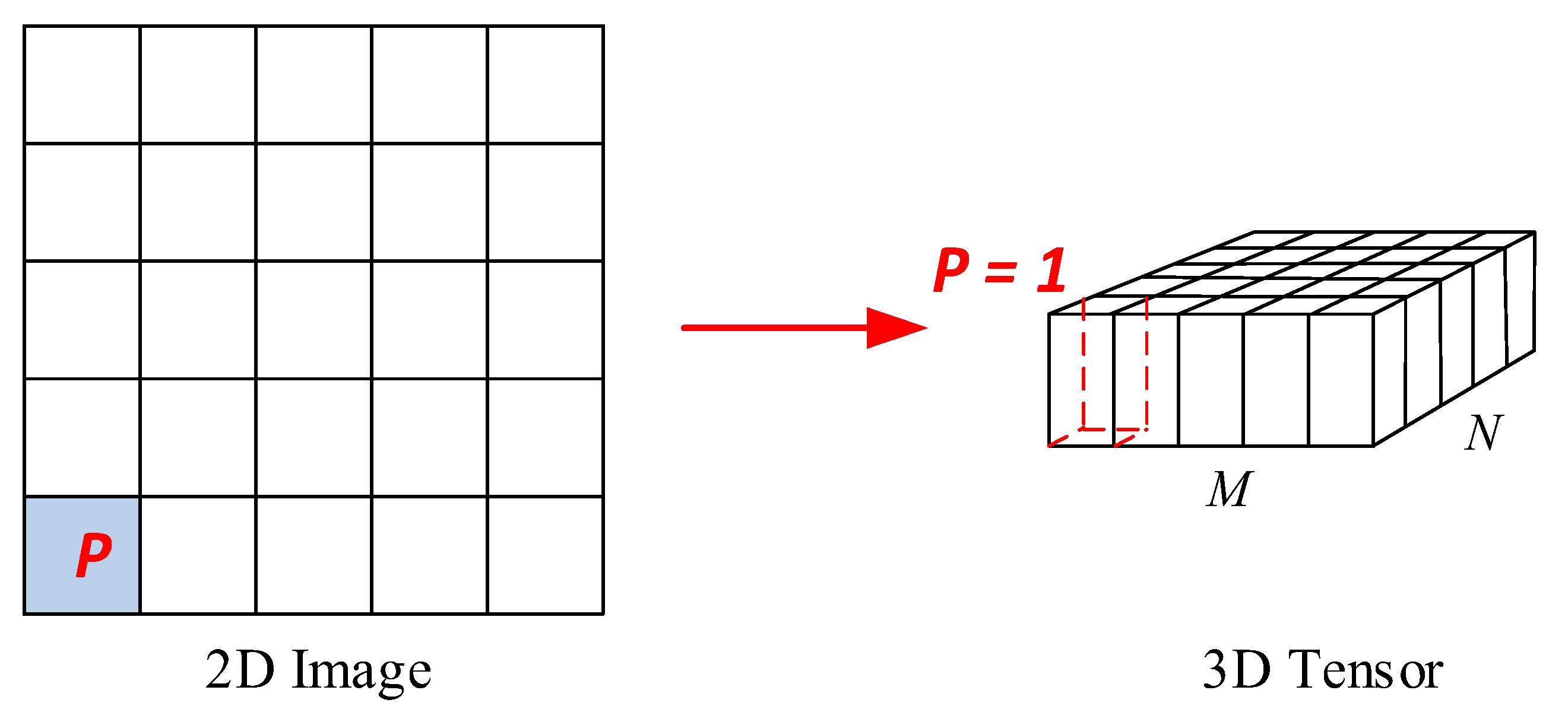
2.1. SST Prediction Using Deep Learning

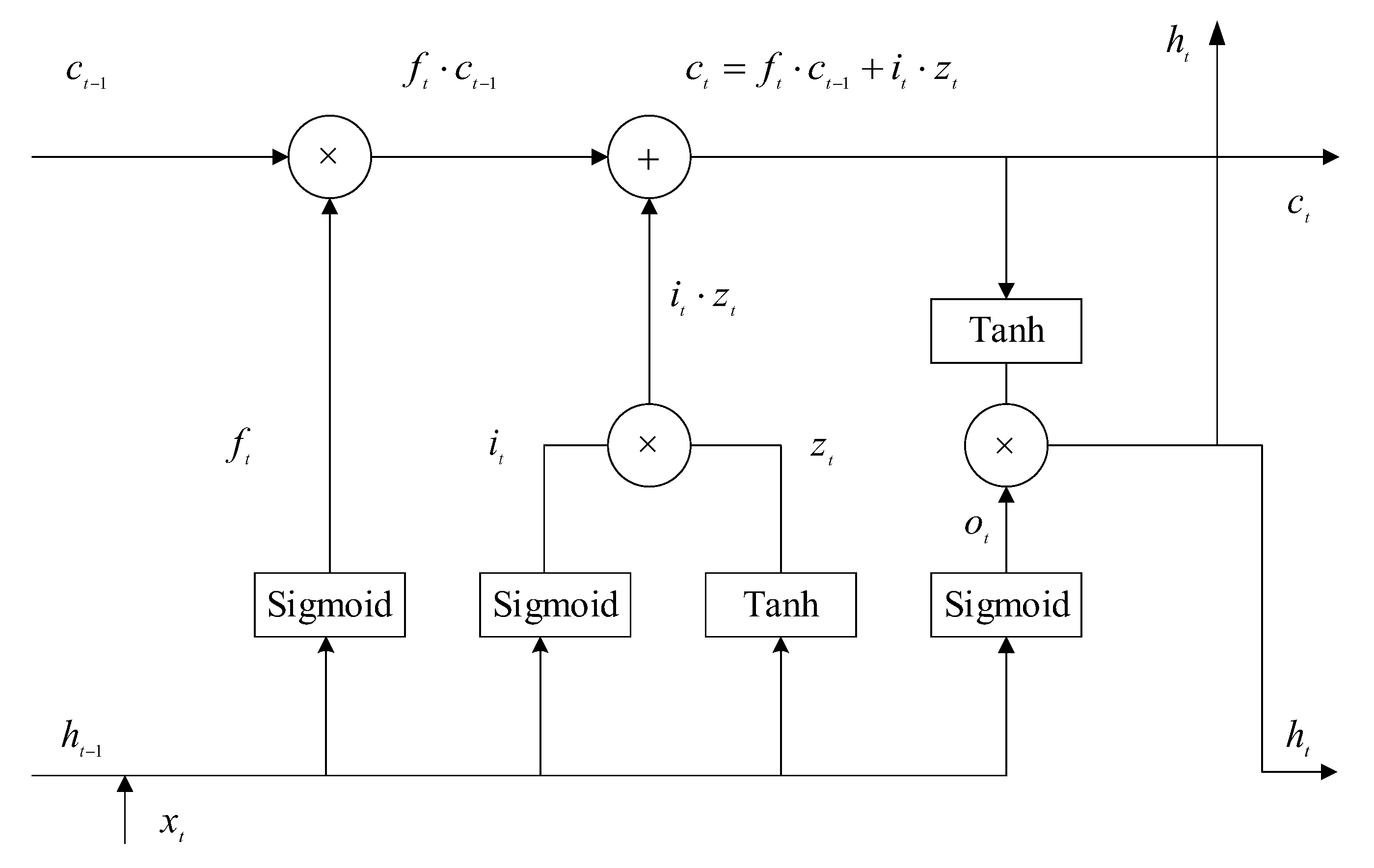
2.2. Long Short-Term Memory
3. Materials and Methods
3.1. Data
3.2. Methods
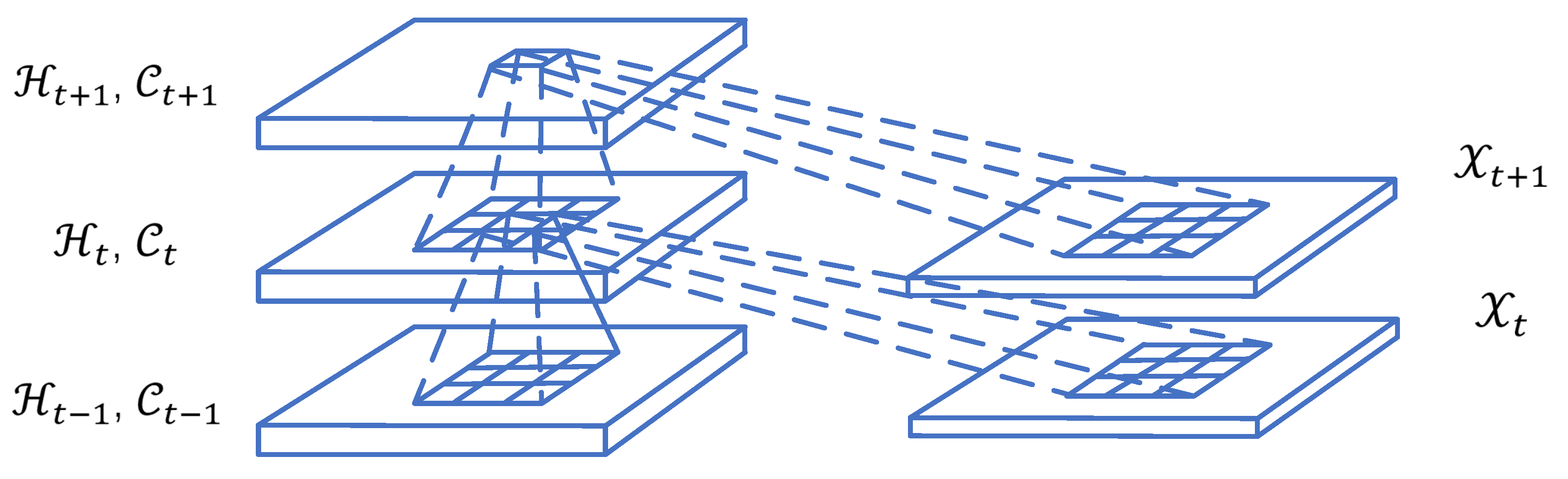
3.2.1. ConvLSTM
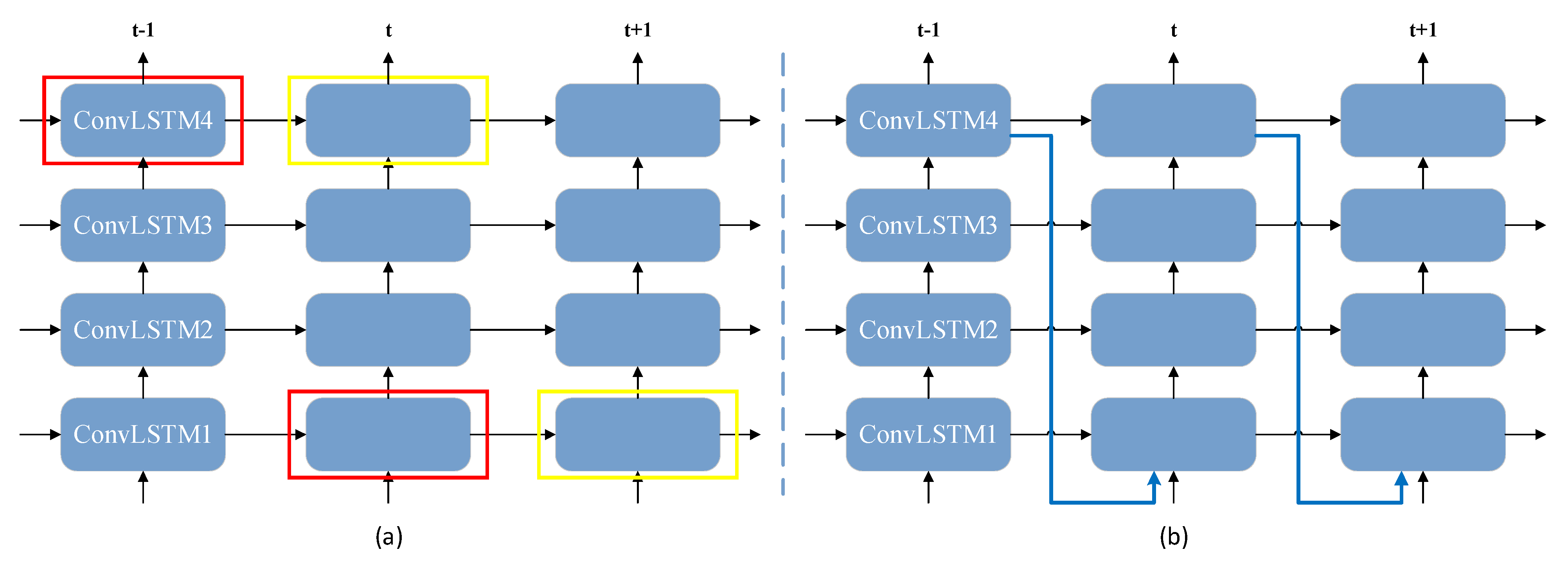
3.2.2. ST-ConvLSTM
4. Experimental Design
4.1. Experimental Environment
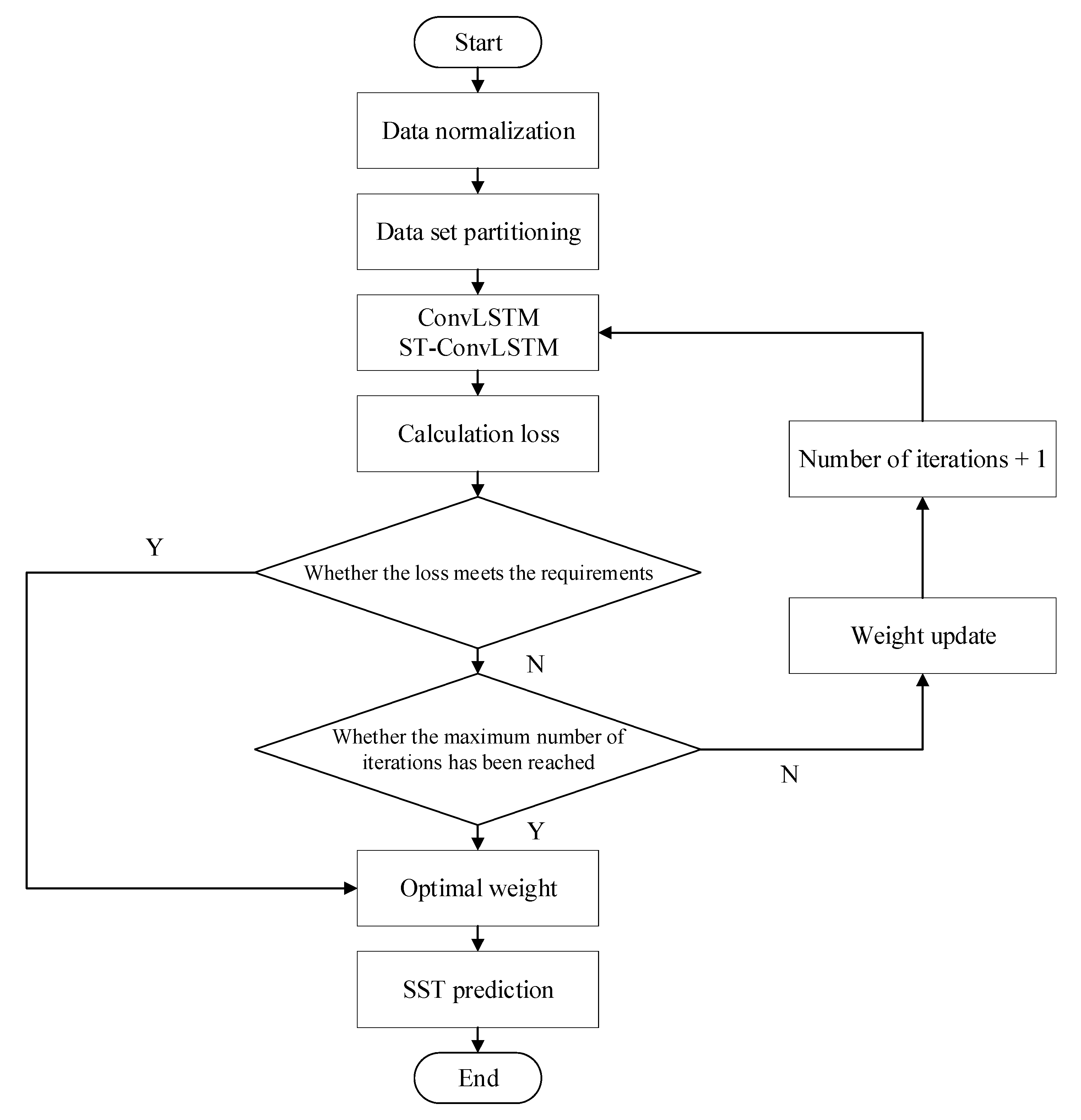
4.2. Experimental Procedures
- Data preprocessing, using the Numpy library to normalize the input data.
- Divide the data, using the data from 2015 to 2018 as the training set and the data in 2019 as the validation set.
- Set a fixed random seed to ensure that each experiment can be reproduced.
- Model training, using the Adam optimization function to iteratively train the model, and automatically save the optimal weight.
- Visualize the experimental results and intuitively compare the SST prediction ability of different methods.
4.3. Metrics
5. Results
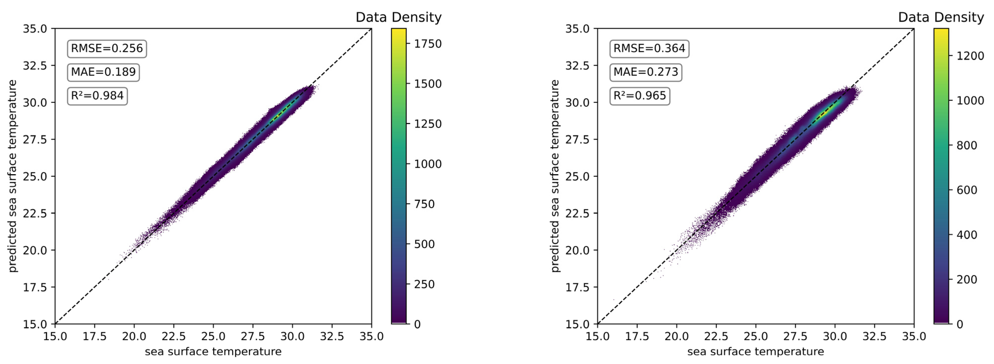
5.1. Effect of Input Length on SST Prediction Performance
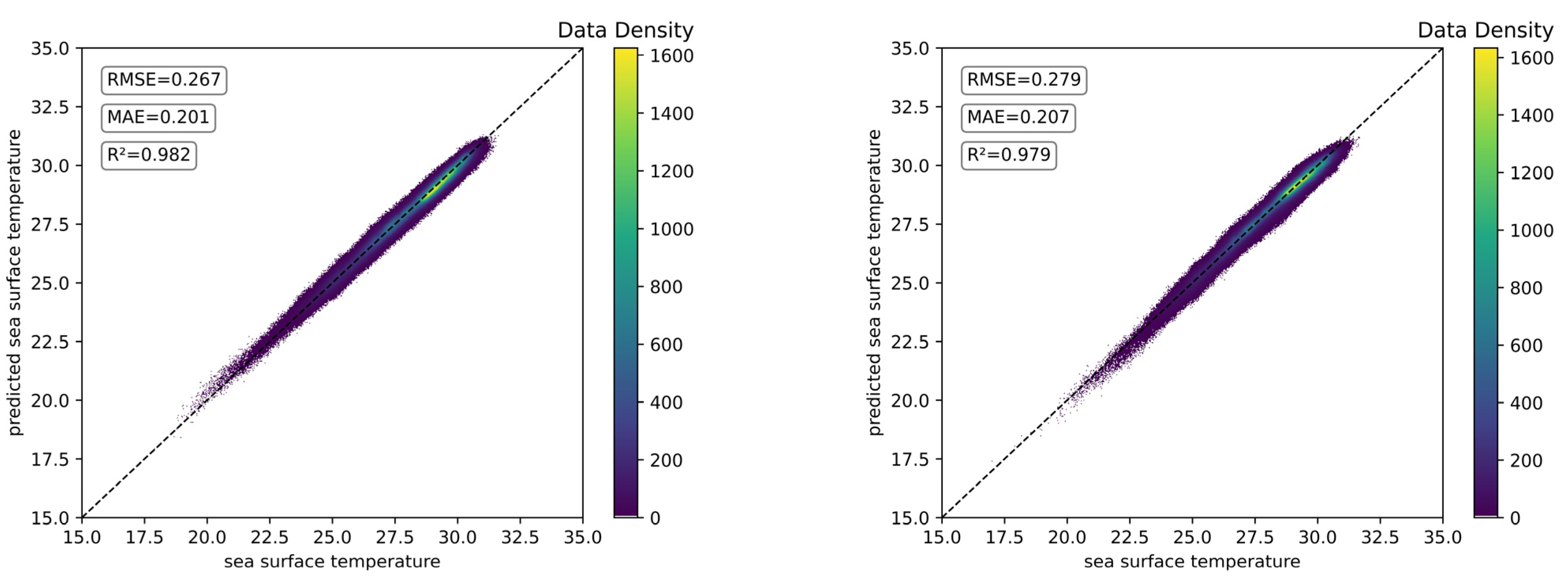
5.2. Effect of Prediction Length on SST Prediction Performance
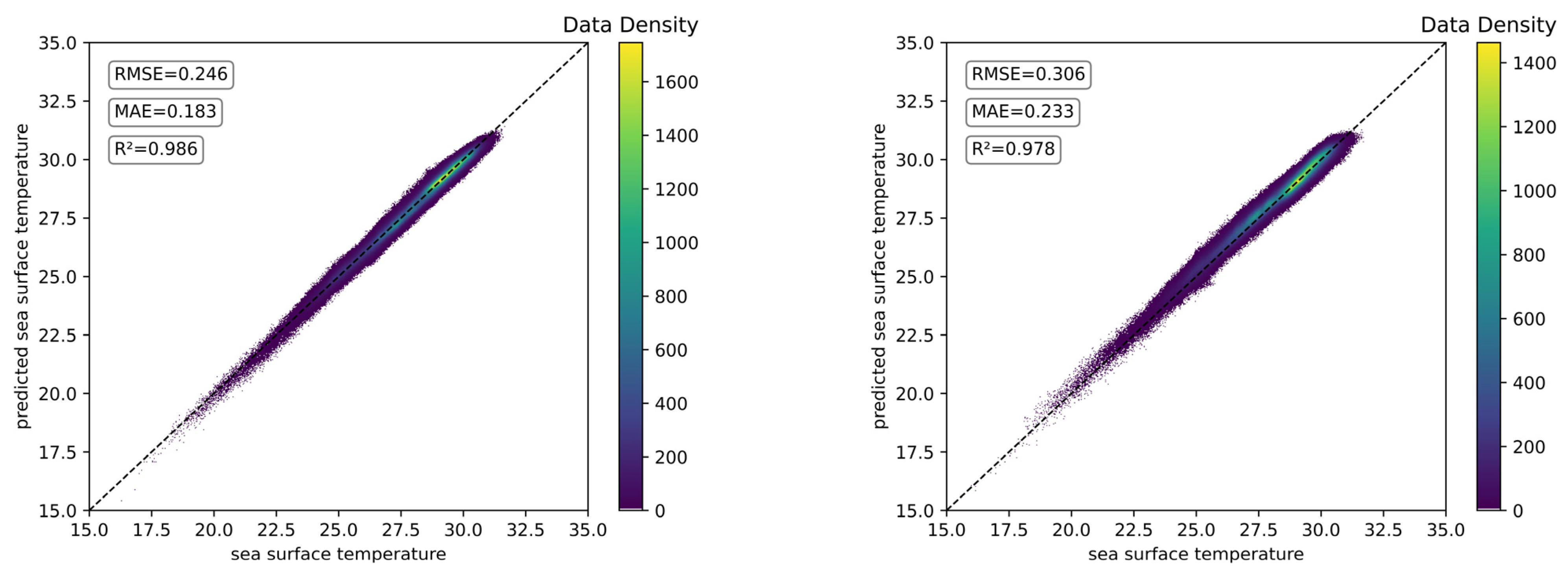
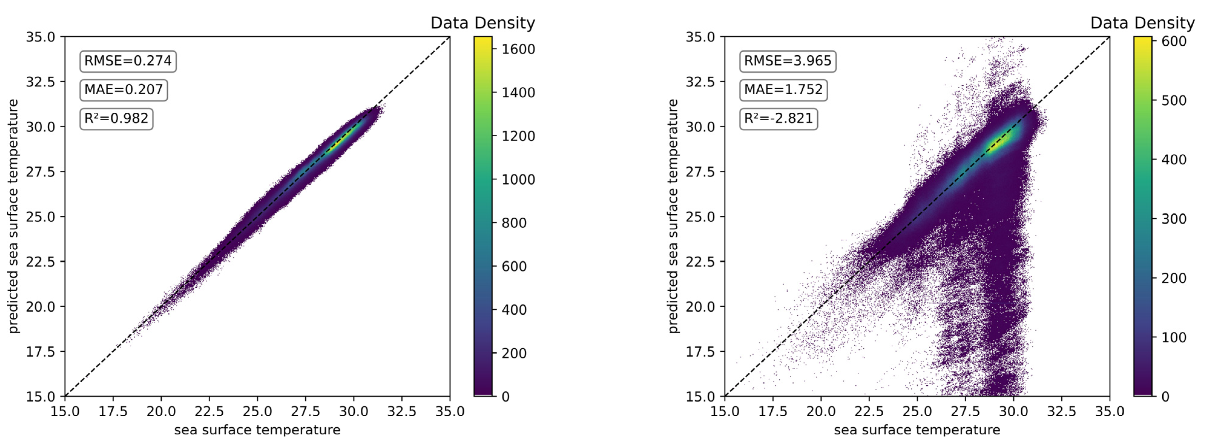
5.3. Effect of Hidden Size on SST Prediction Performance
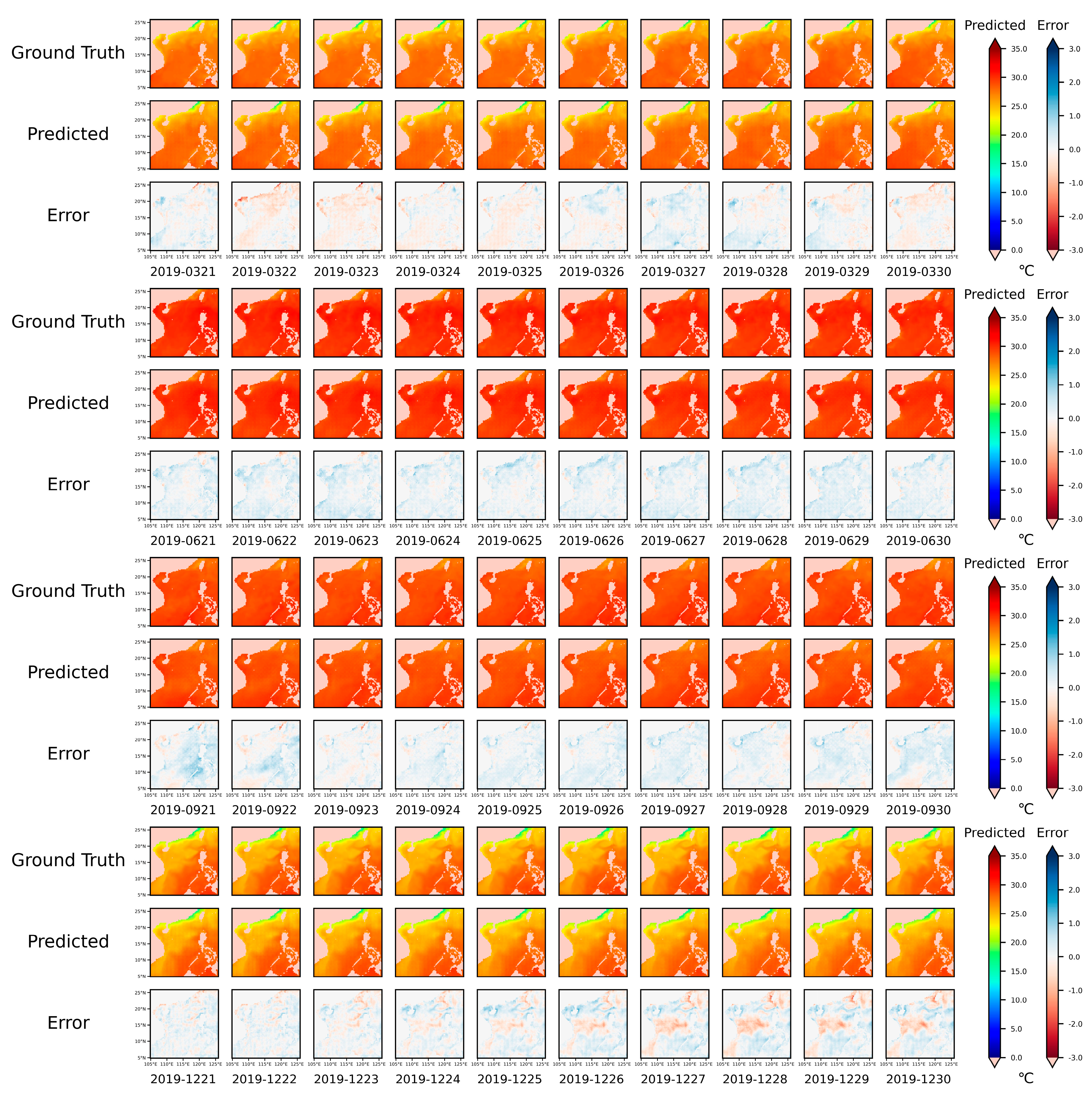
5.4. Visualization of SST Prediction Performance
6. Conclusions
- (1)
- The input length has an effect on SST prediction, but that does not mean that the longer the input length is, the better the prediction performance is. With the same other settings, the two methods, ConvLSTM and ST-ConvLSTM, have the best SST prediction performance when the input length is set to 1. On the whole, the SST prediction performance tends to decrease instead as the input length increases.
- (2)
- The prediction length has an effect on SST prediction. When other parameters are kept constant and only the prediction length is changed, ConvLSTM gets the optimal result when the prediction length is set to 2 and ST-ConvLSTM gets the optimal result when the prediction length is set to 1. The SST prediction performance of ConvLSTM and ST-ConvLSTM tends to decrease gradually as the prediction length increases.
- (3)
- The setting of the hidden size has a large impact on the prediction ability. For ConvLSTM, the prediction performance first gradually improves with the increase in the hidden size value, and the improvement is larger, and then the SST prediction performance starts to decrease when the hidden size is set to 128. For ST-ConvLSTM, the prediction performance gradually improves as the hidden size increases, and the prediction performance of SST is better when the hidden size is set to 128 than when it is set to 64, but then the computational cost increases by about 50% and the performance only improves by about 10%.
Author Contributions
Funding
Data Availability Statement
Conflicts of Interest
References
- Trenberth, K.E.; Branstator, G.W.; Karoly, D.; Kumar, A.; Lau, N.C.; Ropelewski, C. Progress during TOGA in understanding and modeling global teleconnections associated with tropical sea surface temperatures. J. Geophys. Res. Ocean. 1998, 103, 14291–14324. [Google Scholar] [CrossRef]
- Ishii, M.; Shouji, A.; Sugimoto, S.; Matsumoto, T. Objective analyses of sea-surface temperature and marine meteorological variables for the 20th century using ICOADS and the Kobe collection. Int. J. Climatol. J. R. Meteorol. Soc. 2005, 25, 865–879. [Google Scholar] [CrossRef]
- Xie, S.-P.; Deser, C.; Vecchi, G.A.; Ma, J.; Teng, H.; Wittenberg, A.T. Global warming pattern formation: Sea surface temperature and rainfall. J. Clim. 2010, 23, 966–986. [Google Scholar] [CrossRef] [Green Version]
- Donlon, C.; Robinson, I.; Casey, K.; Vazquez-Cuervo, J.; Armstrong, E.; Arino, O.; Gentemann, C.; May, D.; LeBorgne, P.; Piollé, J. The global ocean data assimilation experiment high-resolution sea surface temperature pilot project. Bull. Am. Meteorol. Soc. 2007, 88, 1197–1214. [Google Scholar] [CrossRef]
- Deser, C.; Alexander, M.A.; Xie, S.-P.; Phillips, A.S. Sea surface temperature variability: Patterns and mechanisms. Annu. Rev. Mar. Sci. 2010, 2, 115–143. [Google Scholar] [CrossRef] [Green Version]
- Kennedy, J.J.; Rayner, N.; Atkinson, C.; Killick, R. An ensemble data set of sea surface temperature change from 1850: The Met Office Hadley Centre HadSST. 4.0. 0.0 data set. J. Geophys. Res. Atmos. 2019, 124, 7719–7763. [Google Scholar] [CrossRef]
- Kilpatrick, K.; Podesta, G.; Evans, R. Overview of the NOAA/NASA advanced very high resolution radiometer Pathfinder algorithm for sea surface temperature and associated matchup database. J. Geophys. Res. Oceans 2001, 106, 9179–9197. [Google Scholar] [CrossRef]
- Oliver, E.C.; Benthuysen, J.A.; Darmaraki, S.; Donat, M.G.; Hobday, A.J.; Holbrook, N.J.; Schlegel, R.W.; Sen Gupta, A. Marine heatwaves. Ann. Rev. Mar. Sci. 2021, 13, 313–342. [Google Scholar] [CrossRef]
- Oppo, D.W.; Sun, Y. Amplitude and timing of sea-surface temperature change in the northern South China Sea: Dynamic link to the East Asian monsoon. Geology 2005, 33, 785–788. [Google Scholar] [CrossRef]
- Yu, Y.; Zhang, H.-R.; Jin, J.; Wang, Y. Trends of sea surface temperature and sea surface temperature fronts in the South China Sea during 2003–2017. Acta Oceanol. Sin. 2019, 38, 106–115. [Google Scholar] [CrossRef]
- Fang, G.; Chen, H.; Wei, Z.; Wang, Y.; Wang, X.; Li, C. Trends and interannual variability of the South China Sea surface winds, surface height, and surface temperature in the recent decade. J. Geophys. Res. Ocean. 2006, 111, C11S16. [Google Scholar] [CrossRef] [Green Version]
- Chu, P.C.; Lu, S.; Chen, Y. Temporal and spatial variabilities of the South China Sea surface temperature anomaly. J. Geophys. Res. Ocean. 1997, 102, 20937–20955. [Google Scholar] [CrossRef] [Green Version]
- Qu, T. Role of ocean dynamics in determining the mean seasonal cycle of the South China Sea surface temperature. J. Geophys. Res. Ocean. 2001, 106, 6943–6955. [Google Scholar] [CrossRef]
- Pelejero, C.; Grimalt, J.O. The correlation between the 37k index and sea surface temperatures in the warm boundary: The South China Sea. Geochim. Cosmochim. Acta 1997, 61, 4789–4797. [Google Scholar] [CrossRef]
- Wang, Y.; Yu, Y.; Zhang, Y.; Zhang, H.-R.; Chai, F. Distribution and variability of sea surface temperature fronts in the south China sea. Estuar. Coast. Shelf Sci. 2020, 240, 106793. [Google Scholar] [CrossRef]
- Tan, W.; Wang, X.; Wang, W.; Wang, C.; Zuo, J. Different responses of sea surface temperature in the South China Sea to various El Niño events during boreal autumn. J. Clim. 2016, 29, 1127–1142. [Google Scholar] [CrossRef]
- Lin, C.-Y.; Ho, C.-R.; Zheng, Q.; Huang, S.-J.; Kuo, N.-J. Variability of sea surface temperature and warm pool area in the South China Sea and its relationship to the western Pacific warm pool. J. Oceanogr. 2011, 67, 719–724. [Google Scholar] [CrossRef]
- Yao, Y.; Wang, C. Variations in summer marine heatwaves in the South China Sea. J. Geophys. Res. Ocean. 2021, 126, e2021JC017792. [Google Scholar] [CrossRef]
- Xiao, F.; Wang, D.; Zeng, L.; Liu, Q.-Y.; Zhou, W. Contrasting changes in the sea surface temperature and upper ocean heat content in the South China Sea during recent decades. Clim. Dyn. 2019, 53, 1597–1612. [Google Scholar] [CrossRef]
- Kug, J.S.; Kang, I.S.; Lee, J.Y.; Jhun, J.G. A statistical approach to Indian Ocean sea surface temperature prediction using a dynamical ENSO prediction. Geophys. Res. Lett. 2004, 31, L09212. [Google Scholar] [CrossRef]
- Berliner, L.M.; Wikle, C.K.; Cressie, N. Long-lead prediction of Pacific SSTs via Bayesian dynamic modeling. J. Clim. 2000, 13, 3953–3968. [Google Scholar] [CrossRef]
- Kug, J.-S.; Lee, J.-Y.; Kang, I.-S. Global sea surface temperature prediction using a multimodel ensemble. Mon. Weather Rev. 2007, 135, 3239–3247. [Google Scholar] [CrossRef]
- Repelli, C.A.; Nobre, P. Statistical prediction of sea-surface temperature over the tropical Atlantic. Int. J. Climatol. J. R. Meteorol. Soc. 2004, 24, 45–55. [Google Scholar] [CrossRef]
- Borchert, L.F.; Menary, M.B.; Swingedouw, D.; Sgubin, G.; Hermanson, L.; Mignot, J. Improved decadal predictions of North Atlantic subpolar gyre SST in CMIP6. Geophys. Res. Lett. 2021, 48, e2020GL091307. [Google Scholar] [CrossRef]
- Colman, A.; Davey, M. Statistical prediction of global sea-surface temperature anomalies. Int. J. Climatol. J. R. Meteorol. Soc. 2003, 23, 1677–1697. [Google Scholar] [CrossRef]
- Barnett, T.; Graham, N.; Pazan, S.; White, W.; Latif, M.; Flügel, M. ENSO and ENSO-related predictability. Part I: Prediction of equatorial Pacific sea surface temperature with a hybrid coupled ocean–atmosphere model. J. Clim. 1993, 6, 1545–1566. [Google Scholar] [CrossRef]
- Davis, R.E. Predictability of sea surface temperature and sea level pressure anomalies over the North Pacific Ocean. J. Phys. Oceanogr. 1976, 6, 249–266. [Google Scholar] [CrossRef]
- Alexander, M.A.; Matrosova, L.; Penland, C.; Scott, J.D.; Chang, P. Forecasting Pacific SSTs: Linear inverse model predictions of the PDO. J. Clim. 2008, 21, 385–402. [Google Scholar] [CrossRef] [Green Version]
- Gao, G.; Marin, M.; Feng, M.; Yin, B.; Yang, D.; Feng, X.; Ding, Y.; Song, D. Drivers of marine heatwaves in the East China Sea and the South Yellow Sea in three consecutive summers during 2016–2018. J. Geophys. Res. Ocean. 2020, 125, e2020JC016518. [Google Scholar] [CrossRef]
- Costa, P.; Gómez, B.; Venâncio, A.; Pérez, E.; Pérez-Muñuzuri, V. Using the Regional Ocean Modelling System (ROMS) to improve the sea surface temperature predictions of the MERCATOR Ocean System. Sci. Mar. 2012, 76, 165–175. [Google Scholar] [CrossRef] [Green Version]
- Xue, Y.; Leetmaa, A. Forecasts of tropical Pacific SST and sea level using a Markov model. Geophys. Res. Lett. 2000, 27, 2701–2704. [Google Scholar] [CrossRef] [Green Version]
- Collins, D.; Reason, C.; Tangang, F. Predictability of Indian Ocean sea surface temperature using canonical correlation analysis. Clim. Dyn. 2004, 22, 481–497. [Google Scholar] [CrossRef]
- Patil, K.; Deo, M.; Ravichandran, M. Prediction of sea surface temperature by combining numerical and neural techniques. J. Atmos. Ocean. Technol. 2016, 33, 1715–1726. [Google Scholar] [CrossRef]
- Wolff, S.; O’Donncha, F.; Chen, B. Statistical and machine learning ensemble modelling to forecast sea surface temperature. J. Mar. Syst. 2020, 208, 103347. [Google Scholar] [CrossRef]
- Yang, Y.; Dong, J.; Sun, X.; Lima, E.; Mu, Q.; Wang, X. A CFCC-LSTM model for sea surface temperature prediction. IEEE Geosci. Remote Sens. Lett. 2017, 15, 207–211. [Google Scholar] [CrossRef]
- Zhang, Q.; Wang, H.; Dong, J.; Zhong, G.; Sun, X. Prediction of sea surface temperature using long short-term memory. IEEE Geosci. Remote Sens. Lett. 2017, 14, 1745–1749. [Google Scholar] [CrossRef] [Green Version]
- Xiao, C.; Chen, N.; Hu, C.; Wang, K.; Gong, J.; Chen, Z. Short and mid-term sea surface temperature prediction using time-series satellite data and LSTM-AdaBoost combination approach. Remote Sens. Environ. 2019, 233, 111358. [Google Scholar] [CrossRef]
- Hou, S.; Li, W.; Liu, T.; Zhou, S.; Guan, J.; Qin, R.; Wang, Z. MIMO: A Unified Spatio-Temporal Model for Multi-Scale Sea Surface Temperature Prediction. Remote Sens. 2022, 14, 2371. [Google Scholar] [CrossRef]
- Wei, L.; Guan, L.; Qu, L.; Guo, D. Prediction of sea surface temperature in the China seas based on long short-term memory neural networks. Remote Sens. 2020, 12, 2697. [Google Scholar] [CrossRef]
- Cho, K.; Van Merriënboer, B.; Gulcehre, C.; Bahdanau, D.; Bougares, F.; Schwenk, H.; Bengio, Y. Learning phrase representations using RNN encoder-decoder for statistical machine translation. arXiv 2014, arXiv:1406.1078. [Google Scholar]
- Hochreiter, S.; Schmidhuber, J. Long short-term memory. Neural Comput. 1997, 9, 1735–1780. [Google Scholar] [CrossRef]
- Jordan, M.I. Serial order: A parallel distributed processing approach. In Advances in Psychology; Elsevier: Amsterdam, The Netherlands, 1997; Volume 121, pp. 471–495. [Google Scholar]
- Xie, J.; Zhang, J.; Yu, J.; Xu, L. An adaptive scale sea surface temperature predicting method based on deep learning with attention mechanism. IEEE Geosci. Remote Sens. Lett. 2019, 17, 740–744. [Google Scholar] [CrossRef]
- Xu, S.; Dai, D.; Cui, X.; Yin, X.; Jiang, S.; Pan, H.; Wang, G. A deep learning approach to predict sea surface temperature based on multiple modes. Ocean Model. 2023, 181, 102158. [Google Scholar] [CrossRef]
- Shao, Q.; Li, W.; Han, G.; Hou, G.; Liu, S.; Gong, Y.; Qu, P. A deep learning model for forecasting sea surface height anomalies and temperatures in the South China Sea. J. Geophys. Res. Ocean. 2021, 126, e2021JC017515. [Google Scholar] [CrossRef]
- Kim, M.; Yang, H.; Kim, J. Sea surface temperature and high water temperature occurrence prediction using a long short-term memory model. Remote Sens. 2020, 12, 3654. [Google Scholar] [CrossRef]
- Shi, X.; Chen, Z.; Wang, H.; Yeung, D.-Y.; Wong, W.-K.; Woo, W.-C. Convolutional LSTM network: A machine learning approach for precipitation nowcasting. Adv. Neural Inf. Process. Syst. 2015, 28. [Google Scholar] [CrossRef]
- Wang, Y.; Long, M.; Wang, J.; Gao, Z.; Yu, P.S. Predrnn: Recurrent neural networks for predictive learning using spatiotemporal lstms. Adv. Neural Inform. Process. Syst. 2017, 30. [Google Scholar]
- Li, C.; Feng, Y.; Sun, T.; Zhang, X. Long term Indian Ocean Dipole (IOD) index prediction used deep learning by convLSTM. Remote Sens. 2022, 14, 523. [Google Scholar] [CrossRef]
- Zhang, K.; Geng, X.; Yan, X.-H. Prediction of 3-D ocean temperature by multilayer convolutional LSTM. IEEE Geosci. Remote Sens. Lett. 2020, 17, 1303–1307. [Google Scholar] [CrossRef]
- Xiao, C.; Chen, N.; Hu, C.; Wang, K.; Xu, Z.; Cai, Y.; Xu, L.; Chen, Z.; Gong, J. A spatiotemporal deep learning model for sea surface temperature field prediction using time-series satellite data. Environ. Model. Softw. 2019, 120, 104502. [Google Scholar] [CrossRef]
- De Mattos Neto, P.S.; Cavalcanti, G.D.; de O Santos Júnior, D.S.; Silva, E.G. Hybrid systems using residual modeling for sea surface temperature forecasting. Sci. Rep. 2022, 12, 487. [Google Scholar] [CrossRef]
- Qiao, B.; Wu, Z.; Ma, L.; Zhou, Y.; Sun, Y. Effective ensemble learning approach for SST field prediction using attention-based PredRNN. Front. Comput. Sci. 2023, 17, 171601. [Google Scholar] [CrossRef]
- Kingma, D.P.; Ba, J. Adam: A method for stochastic optimization. arXiv 2014, arXiv:1412.6980. [Google Scholar]
- Paszke, A.; Gross, S.; Massa, F.; Lerer, A.; Bradbury, J.; Chanan, G.; Killeen, T.; Lin, Z.; Gimelshein, N.; Antiga, L. Pytorch: An imperative style, high-performance deep learning library. Adv. Neural Inform. Process. Syst. 2019, 32. [Google Scholar]


| Input | Time Dimension | Spatial Dimension | Temporal Resolution | Spatial Resolution |
|---|---|---|---|---|
SST | 2015–2019 | 5°N–26°N, 105°E–126°E | Daily Mean | 0.25° × 0.25° |
| Parameter | Setting |
|---|---|
| Input length | 1 / 3 / 5 / 7 / 15 / 30 |
| Prediction length | 1 / 2 / 4 / 6 / 8 / 10 / 15 |
| Hidden size | 2 / 4 / 8 / 16 / 32 / 64 / 128 |
| Layers | 4 |
| Filter size | 3 × 3 |
| Stride | 1 |
| Batch size | 20 |
| Patch size | 5 |
| Test interval | 100 |
| Image size | 85 × 85 |
| Image channel | 1 |
| Input Length | ConvLSTM | ST-ConvLSTM | ||||
|---|---|---|---|---|---|---|
| 1-d 3-d 5-d 7-d 15-d 30-d | 0.2559 0.2864 0.3217 0.3280 0.3683 0.3640 | 0.1885 0.2155 0.2372 0.2481 0.2796 0.2734 | 0.9838 0.9798 0.9745 0.9735 0.9671 0.9646 | 0.2673 0.2799 0.2994 0.3019 0.3384 0.2791 | 0.2008 0.2087 0.2187 0.2290 0.2490 0.2069 | 0.9824 0.9807 0.9779 0.9775 0.9722 0.9792 |
| Prediction Length | ConvLSTM | ST-ConvLSTM | ||||
|---|---|---|---|---|---|---|
| 1-d 2-d 4-d 6-d 8-d 10-d 15-d | 0.2463 0.2443 0.2538 0.2559 0.3031 0.2921 0.3055 | 0.1833 0.1827 0.1895 0.1885 0.2381 0.2202 0.2331 | 0.9856 0.9859 0.9849 0.9838 0.9775 0.9792 0.9776 | 0.2195 0.2287 0.2705 0.2673 0.2717 0.2744 0.3272 | 0.1643 0.1693 0.2029 0.2008 0.2085 0.2065 0.2595 | 0.9886 0.9877 0.9828 0.9824 0.9819 0.9817 0.9743 |
| Hidden Size | ConvLSTM | ST-ConvLSTM | ||||
|---|---|---|---|---|---|---|
| 2 4 8 16 32 64 128 | 4.0448 3.3343 2.5523 1.4760 0.3670 0.2921 0.3226 | 1.8103 1.4934 1.1545 0.7289 0.2825 0.2202 0.2598 | −2.9753 −1.7014 −0.5828 0.4706 0.9672 0.9792 0.9747 | 3.9653 3.3333 2.5377 1.4820 0.2953 0.2744 0.2459 | 1.7515 1.4852 1.1426 0.7500 0.2220 0.2065 0.1821 | −2.8206 −1.6997 −0.5647 0.4662 0.9788 0.9817 0.9852 |
| Time Nodes | ConvLSTM | ST-ConvLSTM | ||
|---|---|---|---|---|
| Max | Min | Max | Min | |
| 21 March 2019~30 March 2019 21 June 2019~30 June 2019 21 September 2019~30 September 2019 21 December 2019~30 December 2019 | 1.5590 1.4458 1.6907 1.6345 | −3.3055 −1.3259 −1.6543 −1.9725 | 2.1003 1.3666 1.3691 2.7281 | −2.5679 −1.2347 −1.4009 −2.3366 |
Disclaimer/Publisher’s Note: The statements, opinions and data contained in all publications are solely those of the individual author(s) and contributor(s) and not of MDPI and/or the editor(s). MDPI and/or the editor(s) disclaim responsibility for any injury to people or property resulting from any ideas, methods, instructions or products referred to in the content. |
© 2023 by the authors. Licensee MDPI, Basel, Switzerland. This article is an open access article distributed under the terms and conditions of the Creative Commons Attribution (CC BY) license (https://creativecommons.org/licenses/by/4.0/).
Share and Cite
Hao, P.; Li, S.; Song, J.; Gao, Y. Prediction of Sea Surface Temperature in the South China Sea Based on Deep Learning. Remote Sens. 2023, 15, 1656. https://doi.org/10.3390/rs15061656
Hao P, Li S, Song J, Gao Y. Prediction of Sea Surface Temperature in the South China Sea Based on Deep Learning. Remote Sensing. 2023; 15(6):1656. https://doi.org/10.3390/rs15061656
Chicago/Turabian StyleHao, Peng, Shuang Li, Jinbao Song, and Yu Gao. 2023. "Prediction of Sea Surface Temperature in the South China Sea Based on Deep Learning" Remote Sensing 15, no. 6: 1656. https://doi.org/10.3390/rs15061656