
Automated Identification of Landfast Sea Ice in the Laptev Sea from the True-Color MODIS Images Using the Method of Deep Learning

Abstract
:1. Introduction
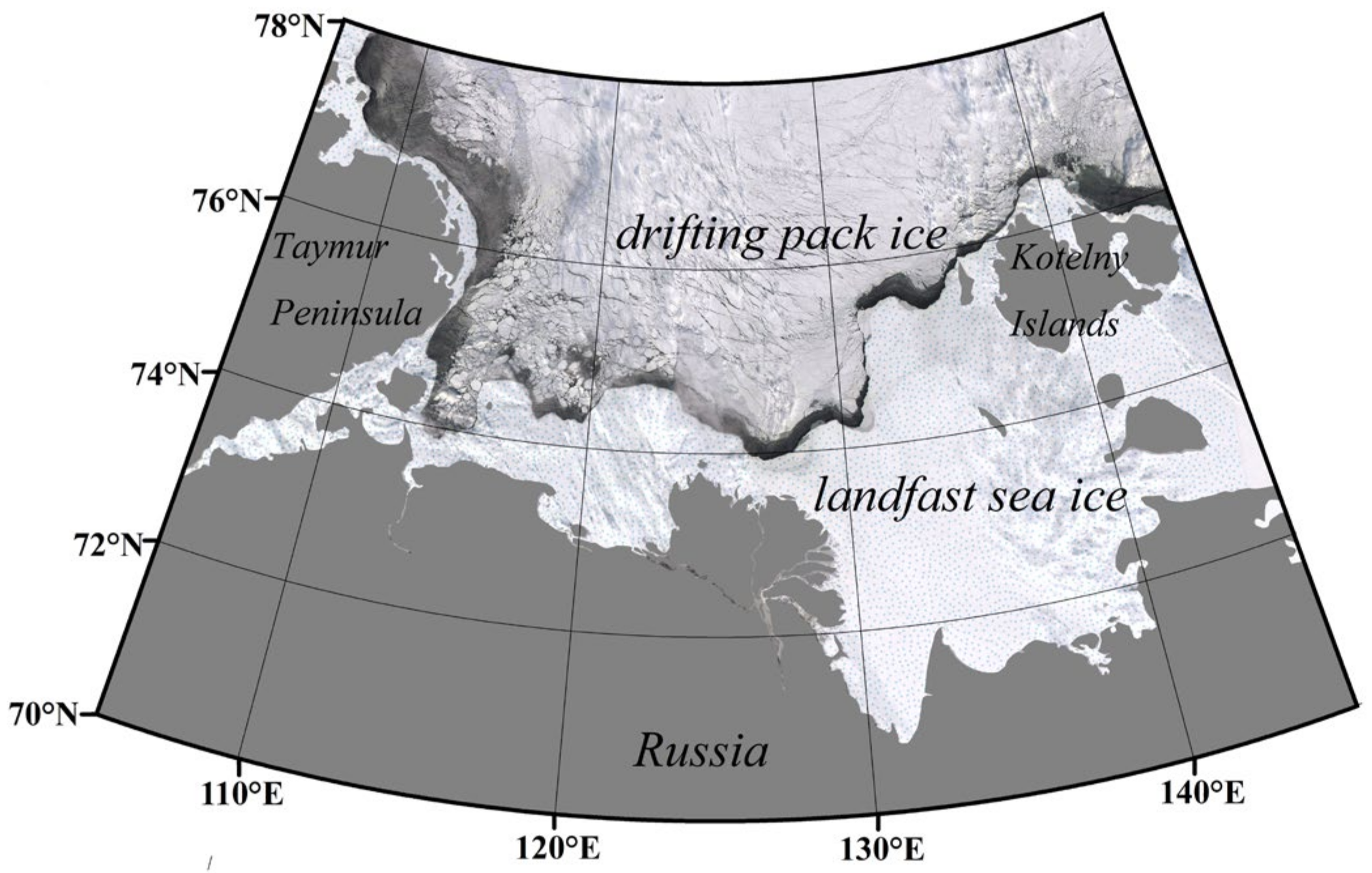
2. Study Area and Data
3. Method
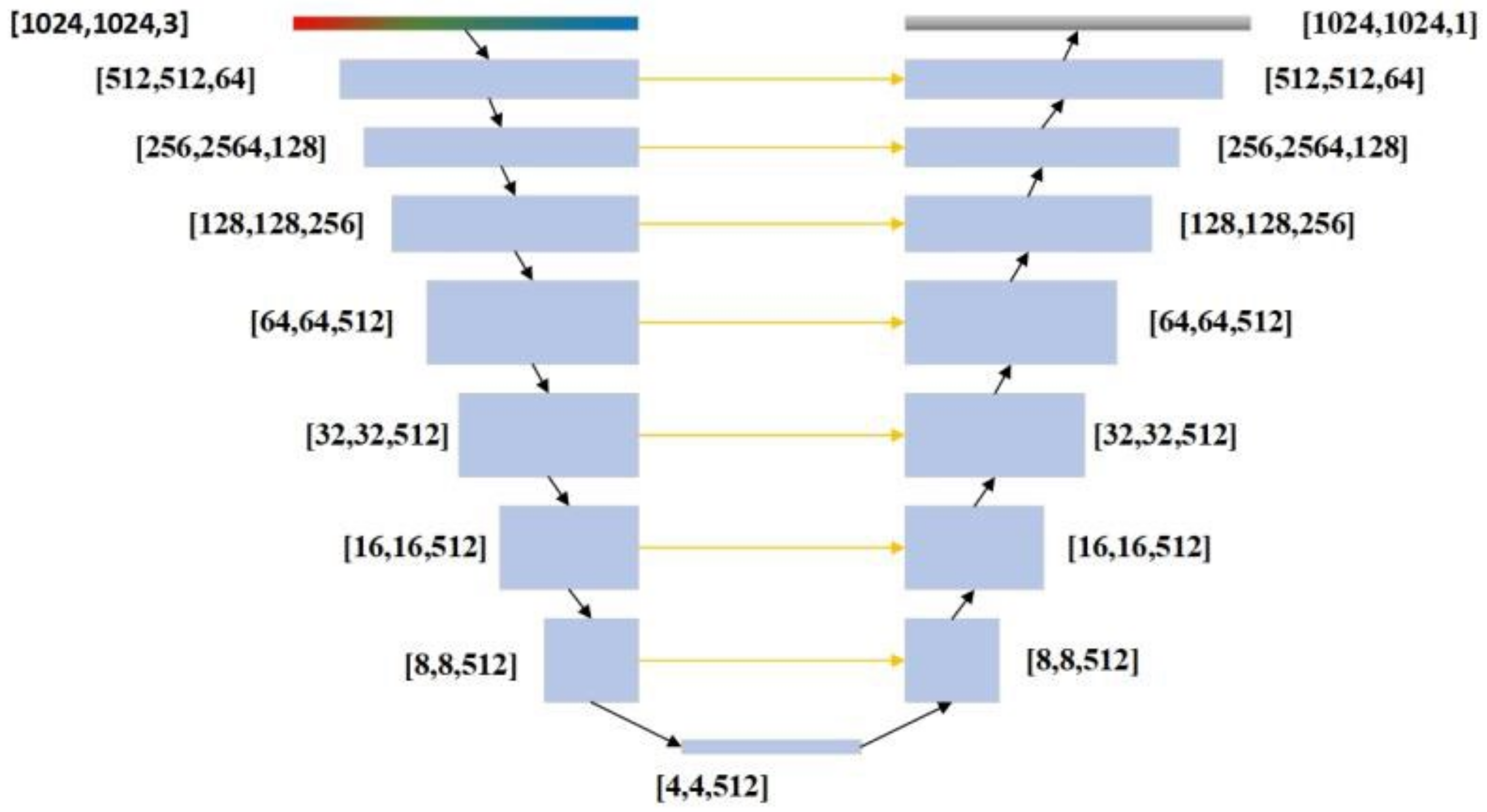
3.1. Pix2Pix Model
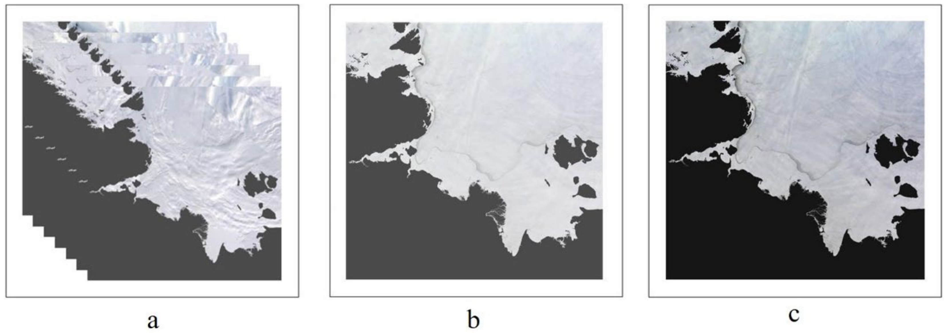
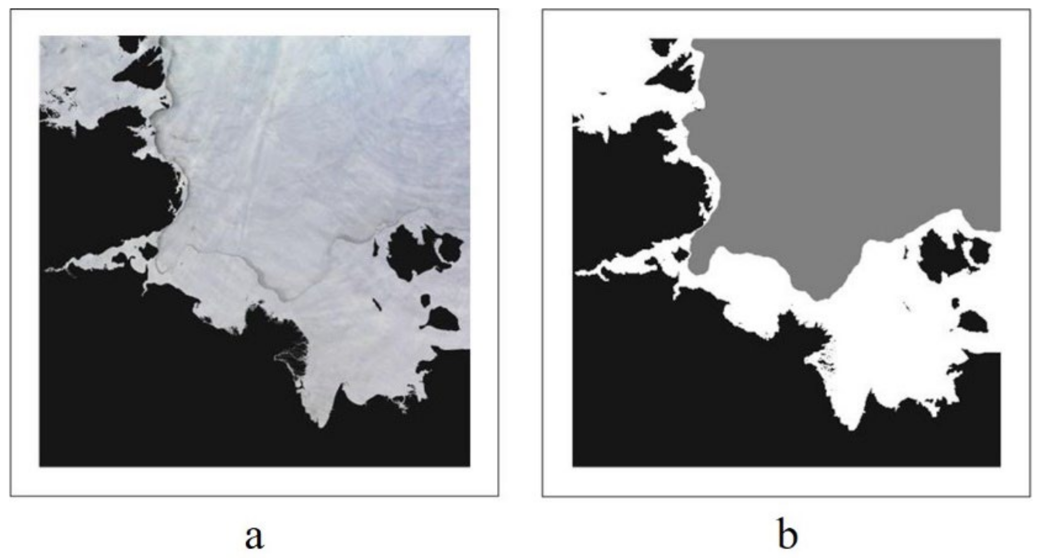
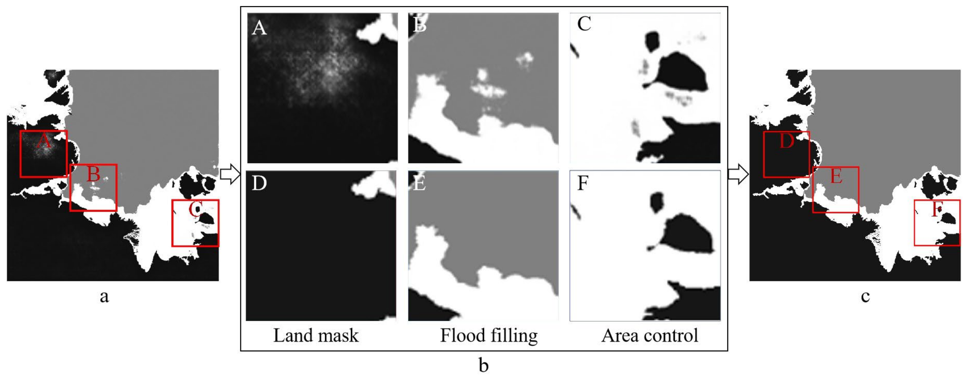
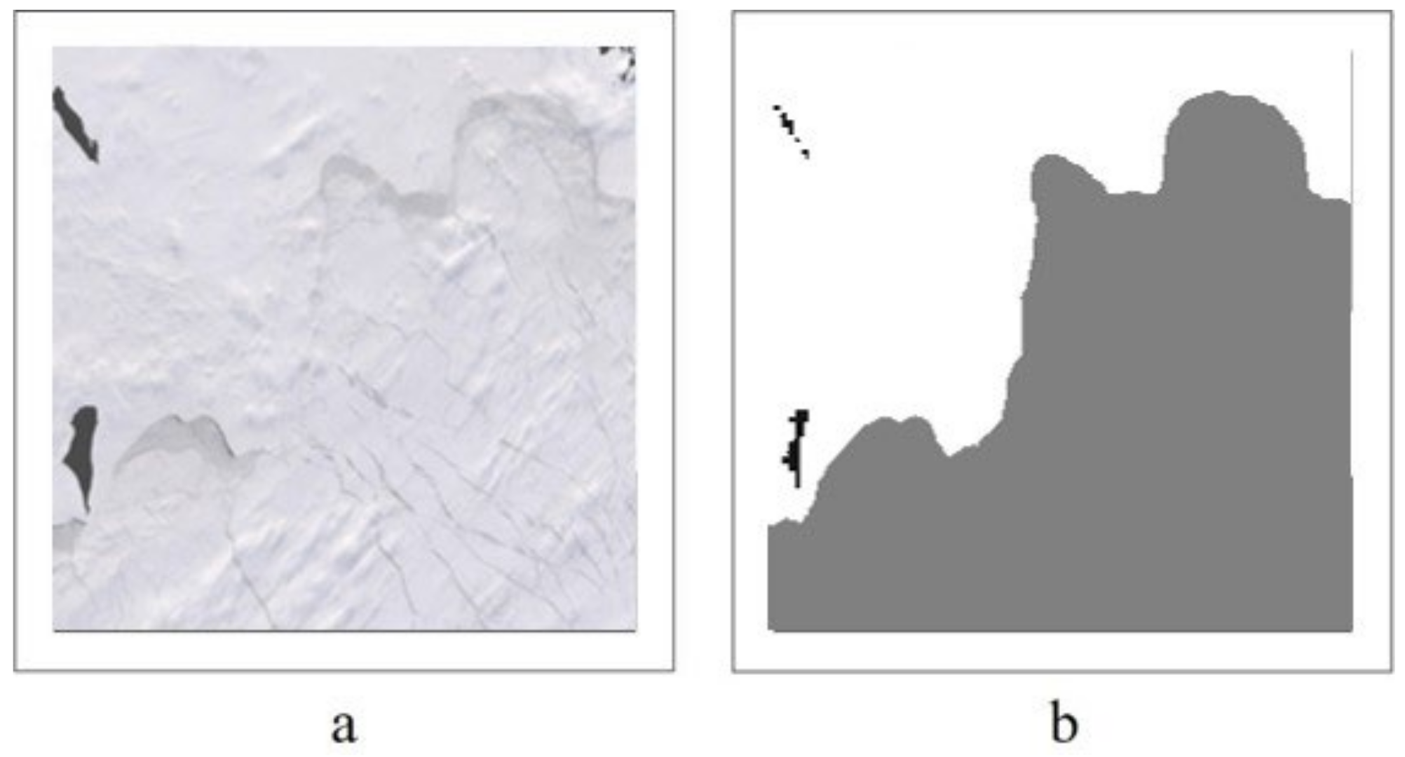
3.2. Image Processing
4. Results and Discussion
4.1. LFSI Mapping Model Performance
4.2. Retrieval of LFSI Area under Cloud Contamination
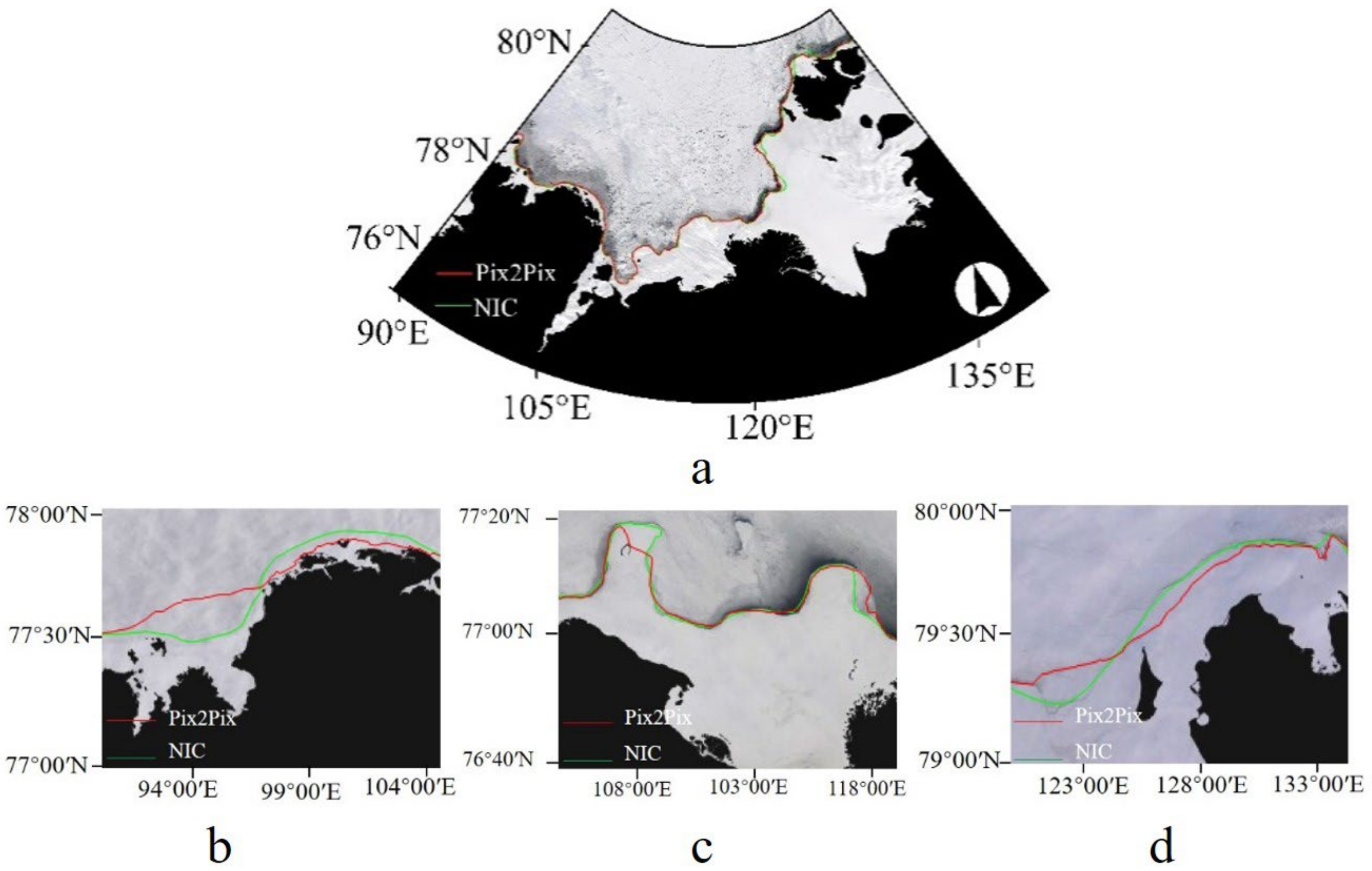
4.3. Comparison with NIC Ice Chart
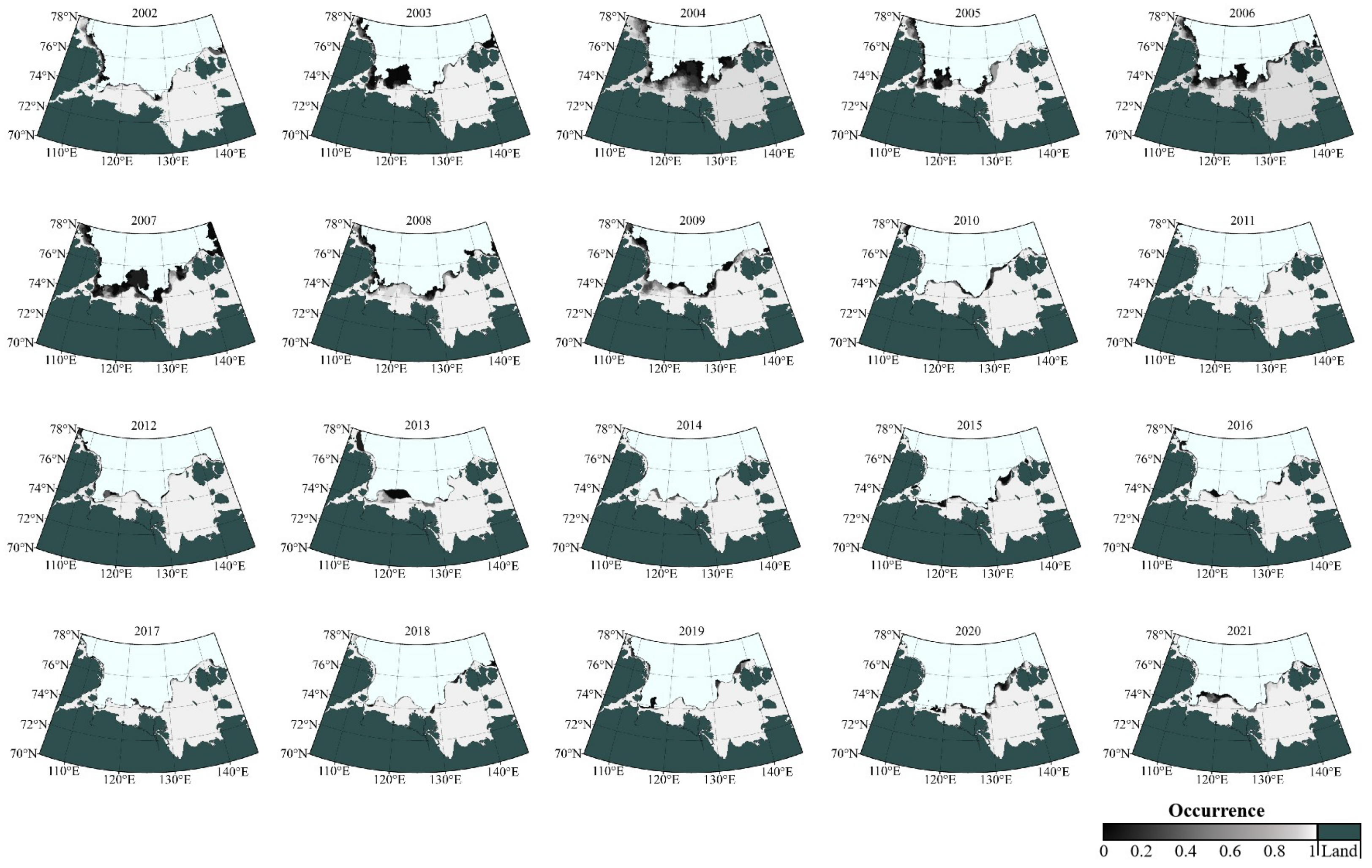
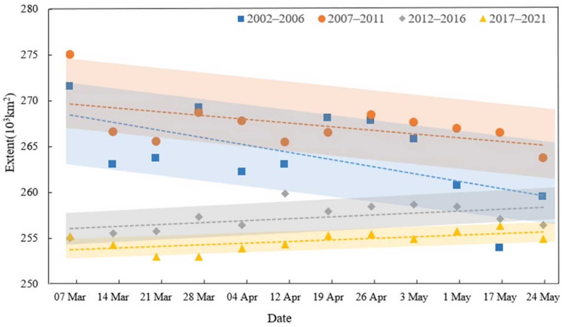
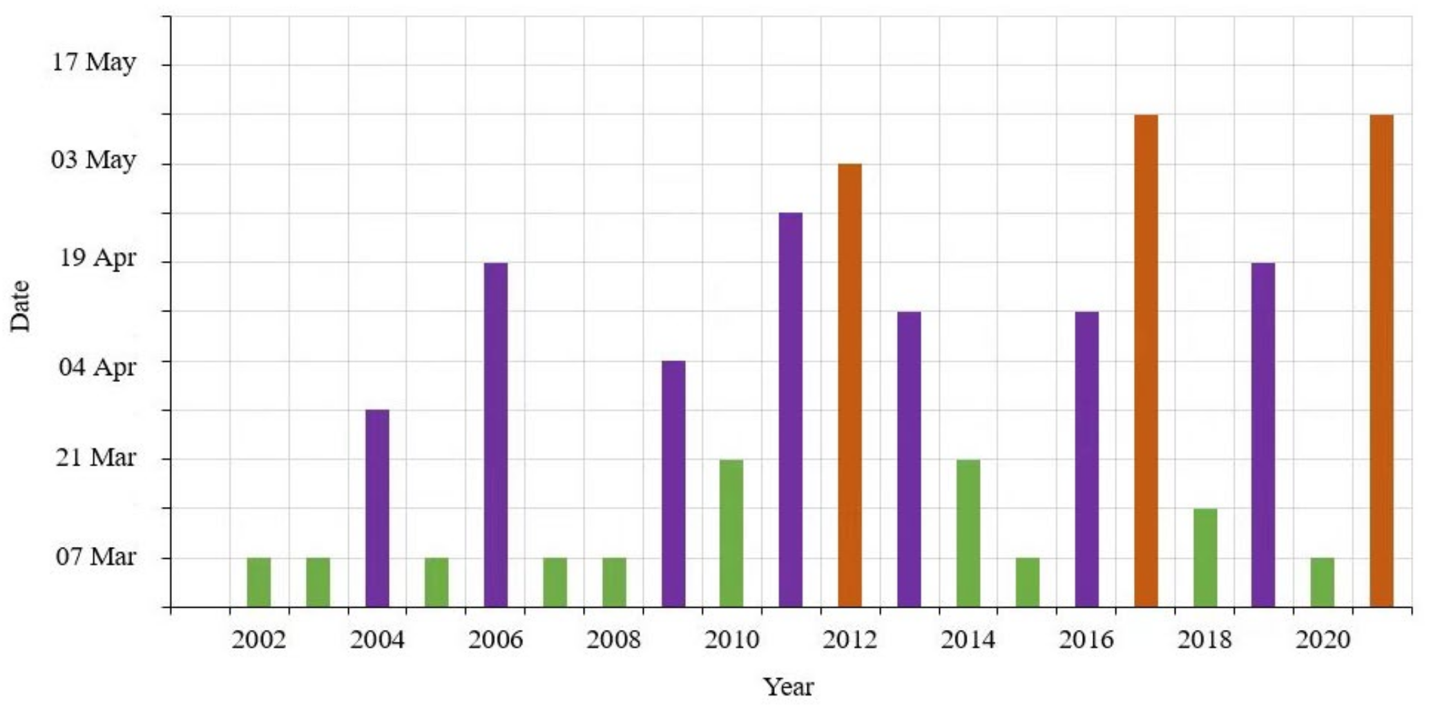
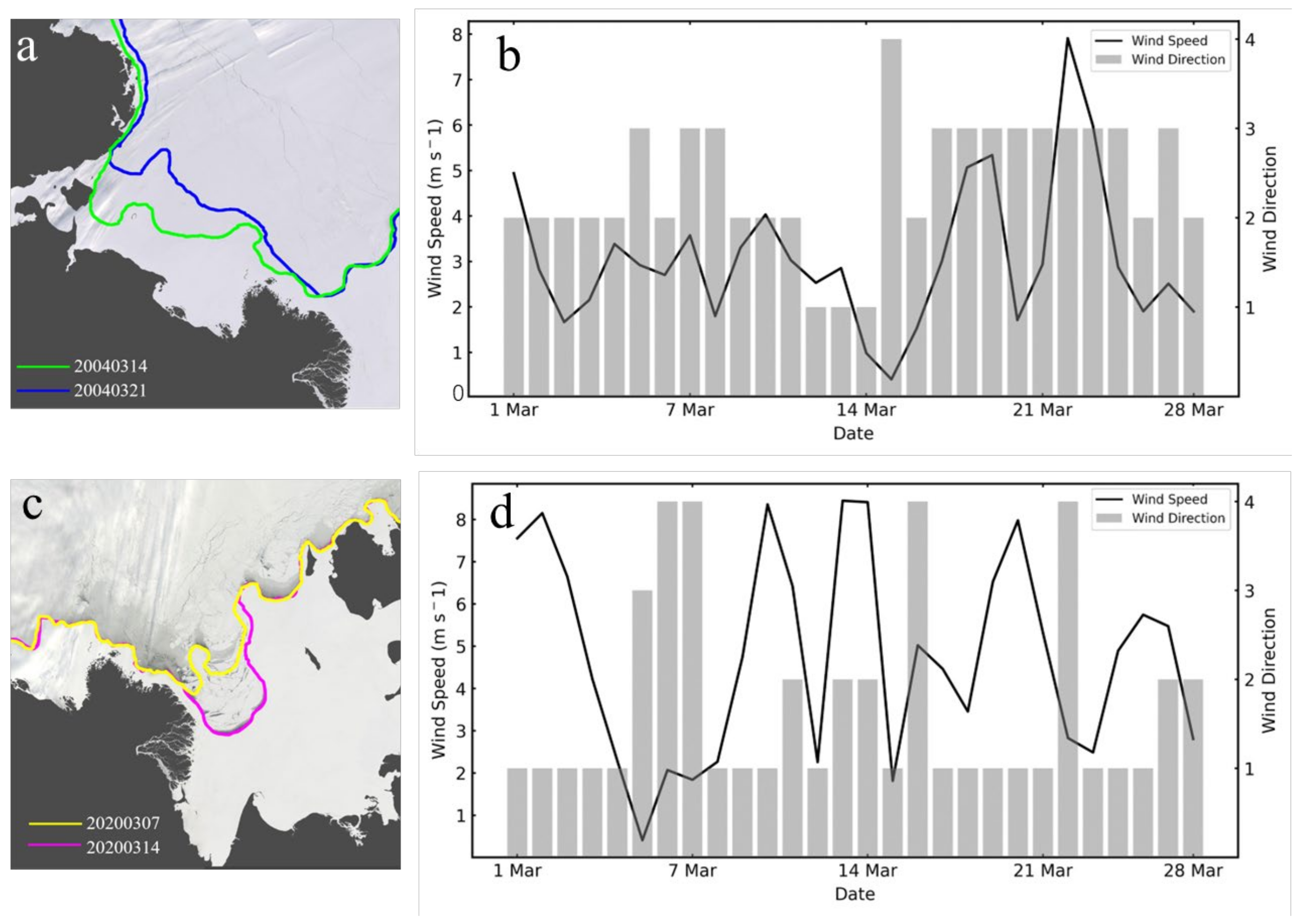
4.4. Spatiotemporal Variation of LFSI in the Laptev Sea
5. Conclusions
Author Contributions
Funding
Acknowledgments
Conflicts of Interest
References
- Cohen, J.; Screen, J.A.; Furtado, J.C.; Barlow, M.; Whittleston, D.; Coumou, D.; Francis, J.; Dethloff, K.; Entekhabi, D.; Overland, J. Recent Arctic amplification and extreme mid-latitude weather. Nat. Geosci. 2014, 7, 627–637. [Google Scholar] [CrossRef] [Green Version]
- Screen, J.A.; Simmonds, I. The central role of diminishing sea ice in recent Arctic temperature amplification. Nature 2010, 464, 1334–1337. [Google Scholar] [CrossRef] [PubMed] [Green Version]
- NSIDC. 2022. Available online: https://climate.nasa.gov/vital-signs/arctic-sea-ice/ (accessed on 1 January 2023).
- Karvonen, J. Estimation of Arctic land-fast ice cover based on dual-polarized Sentinel-1 SAR imagery. Cryosphere 2018, 12, 2595–2607. [Google Scholar] [CrossRef] [Green Version]
- Selyuzhenok, V.; Krumpen, T.; Mahoney, A.R.; Janout, M.A.; Gerdes, R. Seasonal and interannual variability of fast ice extent in the southeastern Laptev Sea between 1999 and 2013. J. Geophys. Res. 2015, 120, 7791–7806. [Google Scholar] [CrossRef] [Green Version]
- Li, Z.; Zhao, J.; Su, J.; Li, C.; Cheng, B.; Hui, F.; Yang, Q.; Shi, L. Spatial and Temporal Variations in the Extent and Thickness of Arctic Landfast Ice. Remote. Sens. 2019, 12, 64. [Google Scholar] [CrossRef] [Green Version]
- Yu, Y.; Stern, H.; Fowler, C.; Fetterer, F.; Maslanik, J. Interannual Variability of Arctic Landfast Ice between 1976 and 2007. J. Clim. 2014, 27, 227–243. [Google Scholar] [CrossRef]
- Massom, R.A.; Giles, A.B.; Fricker, H.A.; Warner, R.C.; Legrésy, B.; Hyland, G.; Young, N.; Fraser, A.D. Examining the interaction between multi-year landfast sea ice and the Mertz Glacier Tongue, East Antarctica: Another factor in ice sheet stability? J. Geophys. Res. 2010, 115, 1–15. [Google Scholar] [CrossRef]
- George, J.C.; Huntington, H.P.; Brewster, K.; Eicken, H.; Norton, D.W.; Glenn, R.P. Observations on Shorefast Ice Dynamics in Arctic Alaska and the Responses of the Iñupiat Hunting Community. Arctic 2004, 57, 363–374. [Google Scholar] [CrossRef]
- Stauffer, G.E.; Rotella, J.J.; Garrott, R.A.; Kendall, W.L. Environmental correlates of temporary emigration for female Weddell seals and consequences for recruitment. Ecology 2014, 95, 2526–2536. [Google Scholar] [CrossRef]
- Labrousse, S.; Fraser, A.D.; Sumner, M.; Le Manach, F.; Sauser, C.; Horstmann, I.; DeVane, E.H.; Delord, K.; Jenouvrier, S.; Barbraud, C. Landfast ice: A major driver of reproductive success in a polar seabird. Biol. Lett. 2021, 17, 20210097. [Google Scholar] [CrossRef]
- Lovvorn, J.R.; Rocha, A.R.; Jewett, S.C.; Dasher, D.; Oppel, S.; Powell, A.N. Limits to benthic feeding by eiders in a vital Arctic migration corridor due to localized prey and chan-ging sea ice. Prog. Oceanogr. 2015, 136, 162–174. [Google Scholar] [CrossRef]
- Selyuzhenok, V.; Mahoney, A.; Krumpen, T.; Castellani, G.; Gerdes, R. Mechanisms of fast-ice development in the south-eastern Laptev Sea: A case study for winter of 2007/08 and 2009/10. Polar Res. 2017, 36, 1411140. [Google Scholar] [CrossRef] [Green Version]
- Olason, E. A dynamical model of Kara Sea land-fast ice. J. Geophys. Res. Ocean. 2016, 121, 3141–3158. [Google Scholar] [CrossRef] [Green Version]
- Divine, D.V.; Korsnes, R.; Makshtas, A.P.; Godtliebsen, F.; Svendsen, H. Atmospheric-driven state transfer of shore-fast ice in the northeastern Kara Sea. J. Geophys. Res. 2005, 110, 1–13. [Google Scholar] [CrossRef] [Green Version]
- Jones, J.; Eicken, H.; Mahoney, A.; Mv, R.; Kambhamettu, C.; Fukamachi, Y.; Ohshima, K.I.; George, J.C. Landfast sea ice breakouts: Stabilizing ice features, oceanic and atmospheric forcing at Barrow, Alaska. Cont. Shelf Res. 2016, 126, 50–63. [Google Scholar] [CrossRef] [Green Version]
- Mahoney, A.R.; Eicken, H.; Graves, A.; Shapiro, L.H.; Cotter, P. Landfast sea ice extent and variability in the Alaskan Arctic derived from SAR imagery. IEEE Int. Geosci. Remote Sens. Symp. 2004, 3, 2146–2149. [Google Scholar]
- Mahoney, A.R.; Eicken, H.; Gaylord, A.G.; Gens, R. Landfast sea ice extent in the Chukchi and Beaufort Seas: The annual cycle and decadal variability. Cold Reg. Sci. Technol. 2014, 103, 41–56. [Google Scholar] [CrossRef]
- Zhai, M.; Cheng, B.; Leppäranta, M.; Hui, F.; Li, X.; Demchev, D. The seasonal cycle and break-up of landfast sea ice along the northwest coast of Kotelny Island, East Siberian Sea. J. Glaciol. 2021, 68, 153–165. [Google Scholar] [CrossRef]
- Fraser, A.D.; Massom, R.A.; Michael, K.J.; Galton-Fenzi, B.K.; Lieser, J.L. East Antarctic Landfast Sea Ice Distribution and Variability, 2000–2008. J. Clim. 2012, 25, 1137–1156. [Google Scholar] [CrossRef] [Green Version]
- Fraser, A.D.; Massom, R.; Ohshima, K.I.; Willmes, S.; Kappes, P.J.; Cartwright, J.; Porter-Smith, R. High-resolution mapping of circum-Antarctic landfast sea ice distribution, 2000–2018. Earth Syst. Sci. Data 2020, 12, 2987–2999. [Google Scholar] [CrossRef]
- Canny, J. A Computational Approach to Edge Detection. IEEE Trans. Pattern Anal. Mach. Intelligence 1986, 8, 679–698. [Google Scholar] [CrossRef]
- Dammann, D.O.; Eriksson, L.E.B.; Mahoney, A.R.; Eicken, H.; Meyer, F.J. Mapping pan-Arctic landfast sea ice stability using Sentinel-1 interferometry. Cryosphere 2019, 13, 557–577. [Google Scholar] [CrossRef] [Green Version]
- Kim, M.; Im, J.; Han, H.; Kim, J.; Lee, S.; Shin, M.; Kim, H.C. Landfast sea ice monitoring using multisensor fusion in the Antarctic. GIScience Remote Sens. 2015, 52, 239–256. [Google Scholar] [CrossRef]
- Chen, Z.; Ting, D.; Newbury, R.; Chen, C. Semantic segmentation for partially occluded apple trees based on deep learning. Comput. Electron. Agric. 2021, 181, 105952. [Google Scholar] [CrossRef]
- Isola, P.; Zhu, J.-Y.; Zhou, T.; Efros, A.A. Image-to-Image Translation with Conditional Adversarial Networks. In Proceedings of the IEEE Conference on Computer Vision and Pattern Recognition (CVPR), Honolulu, HI, USA, 21–26 July 2017; pp. 5676–5967. [Google Scholar]
- Xie, Y.C.; Han, X.Z.; Zhu, S.Y. Synthesis of true color images from the Fengyun Advanced Geostationary Radiation Imager. J. Meteor. Res. 2021, 35, 1136–1147. [Google Scholar] [CrossRef]
- Tsuda, H.; Hotta, K. Cell image segmentation by integrating pix2pixs for each class. In Proceedings of the 2019 IEEE/CVF Conference on Computer Vision and Pattern Recognition Workshops (CVPRW), Long Beach, CA, USA, 16–17 June 2019; pp. 1065–1073. [Google Scholar]
- Ronneberger, O.; Fischer, P.; Brox, T. U-Net: Convolutional Networks for Biomedical Image Segmentation. Med. Image Comput. Comput.-Assist. Interv. MICCAI 2015, 9351, 234–241. [Google Scholar]
- Fraser, A.D.; Massom, R.A.; Michael, K.J. A method for compositing MODIS satellite images to remove cloud cover. IEEE Int. Geosci. Remote Sens. Symp. 2009, 47, 3272–3282. [Google Scholar] [CrossRef]
- Yu, Y.; Leppäanta, M.; Zhijun, L.; Cheng, B.; Mengxi, Z.; Demchev, D. Model simulations of the annual cycle of the landfast ice thickness in the East Siberian Sea. Adv. Polar Sci. 2015, 26, 168–178. [Google Scholar]
- Yang, Y.; Zhijun, L.; Leppäranta, M. Modelling the thickness of landfast sea ice in Prydz Bay, East Antarctica. Antarct. Sci. 2016, 28, 59–70. [Google Scholar] [CrossRef]


| Year | Precision | Recall | F1-Score |
|---|---|---|---|
| 2002 | 0.928 | 0.970 | 0.949 |
| 2003 | 0.903 | 0.988 | 0.951 |
| 2004 | 0.902 | 0.945 | 0.918 |
| 2005 | 0.910 | 0.977 | 0.941 |
| 2006 | 0.909 | 0.980 | 0.943 |
| 2007 | 0.901 | 0.988 | 0.942 |
| 2008 | 0.914 | 0.975 | 0.944 |
| 2009 | 0.920 | 0.985 | 0.951 |
| 2021 | 0.951 | 0.995 | 0.972 |
| Average | 0.914 | 0.979 | 0.945 |
Disclaimer/Publisher’s Note: The statements, opinions and data contained in all publications are solely those of the individual author(s) and contributor(s) and not of MDPI and/or the editor(s). MDPI and/or the editor(s) disclaim responsibility for any injury to people or property resulting from any ideas, methods, instructions or products referred to in the content. |
© 2023 by the authors. Licensee MDPI, Basel, Switzerland. This article is an open access article distributed under the terms and conditions of the Creative Commons Attribution (CC BY) license (https://creativecommons.org/licenses/by/4.0/).
Share and Cite
Wen, C.; Zhai, M.; Lei, R.; Xie, T.; Zhu, J. Automated Identification of Landfast Sea Ice in the Laptev Sea from the True-Color MODIS Images Using the Method of Deep Learning. Remote Sens. 2023, 15, 1610. https://doi.org/10.3390/rs15061610
Wen C, Zhai M, Lei R, Xie T, Zhu J. Automated Identification of Landfast Sea Ice in the Laptev Sea from the True-Color MODIS Images Using the Method of Deep Learning. Remote Sensing. 2023; 15(6):1610. https://doi.org/10.3390/rs15061610
Chicago/Turabian StyleWen, Cheng, Mengxi Zhai, Ruibo Lei, Tao Xie, and Jinshan Zhu. 2023. "Automated Identification of Landfast Sea Ice in the Laptev Sea from the True-Color MODIS Images Using the Method of Deep Learning" Remote Sensing 15, no. 6: 1610. https://doi.org/10.3390/rs15061610