
Effects of Surface Wave-Induced Mixing and Wave-Affected Exchange Coefficients on Tropical Cyclones
 , , and
Abstract
:
1. Introduction
- (1)
- Investigate how wave-induced mixing and wave-affected surface exchange coefficients affect the track, intensity and size of a TC, and analyze air–sea interactions.
- (2)
- Study the combined effects of wave-induced mixing and wave-affected surface exchange coefficients on TCs, including how the impacts of these two factors differ.
2. Background
2.1. Wave-Induced Mixing
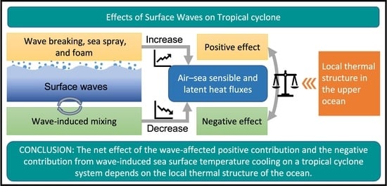
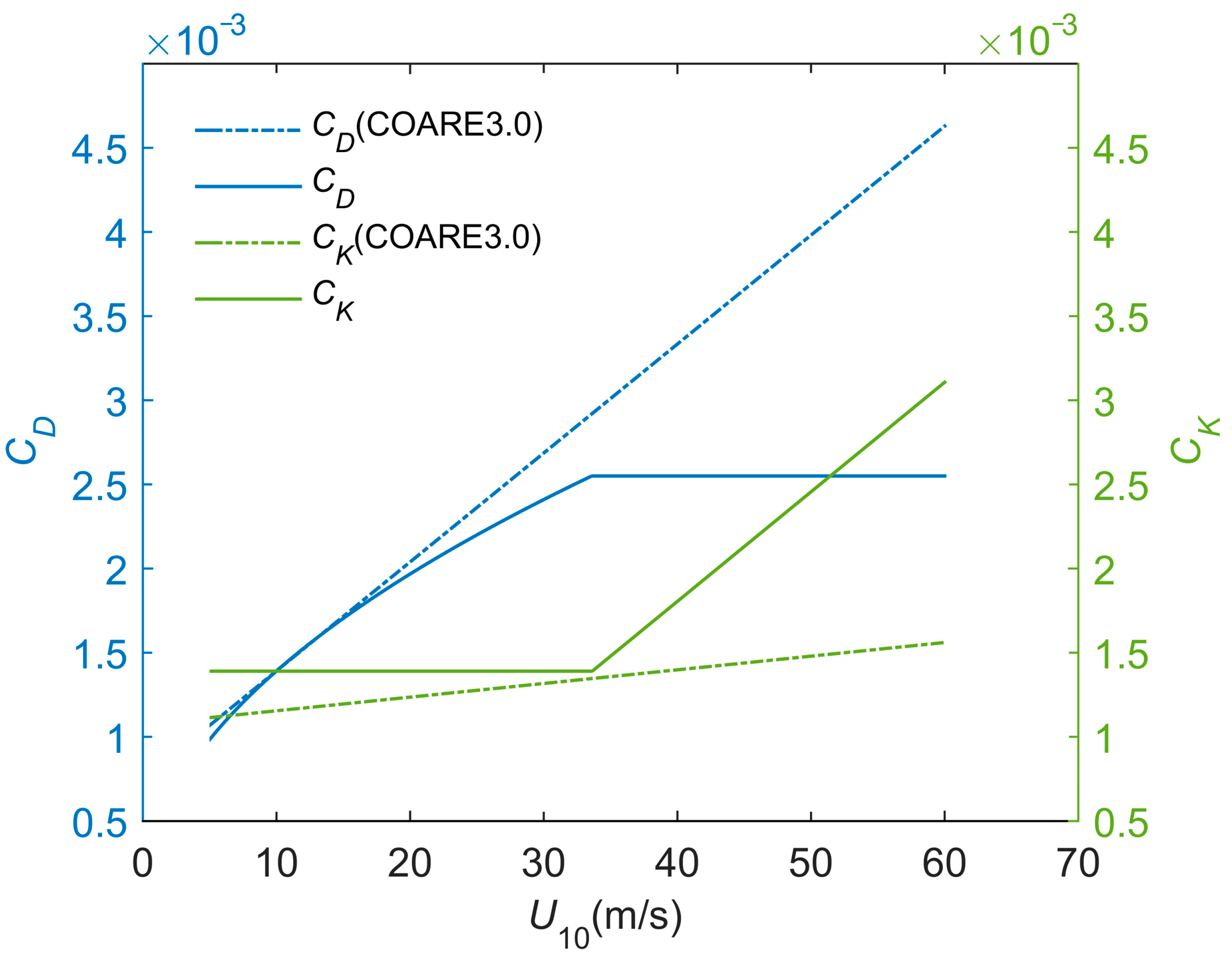
2.2. Wave-Related Small-Scale Processes in the Air–Sea Boundary Layer
3. Materials and Methods
3.1. Experiment Design
3.2. Model Description and Set up
3.3. Data Description
4. Results
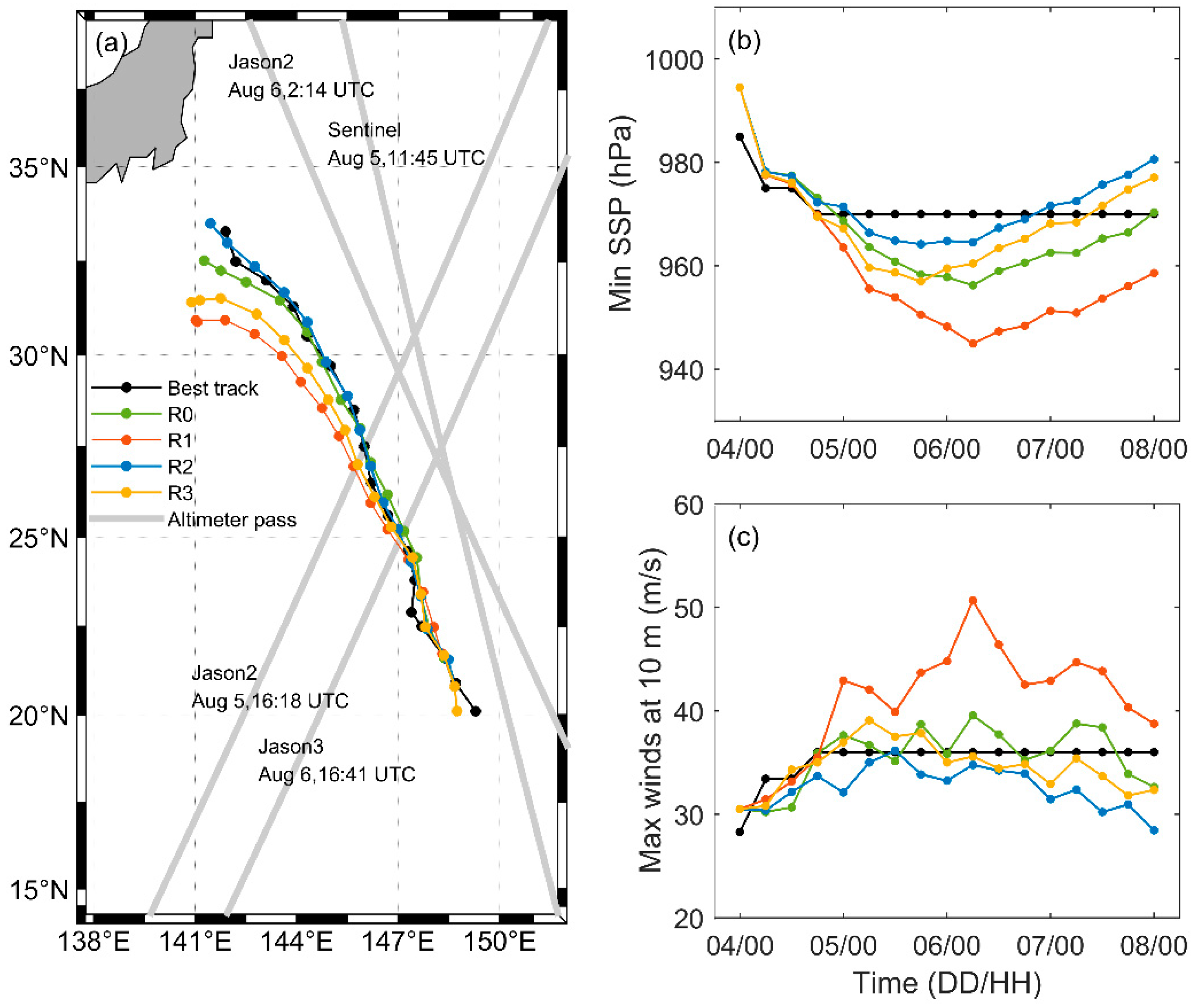
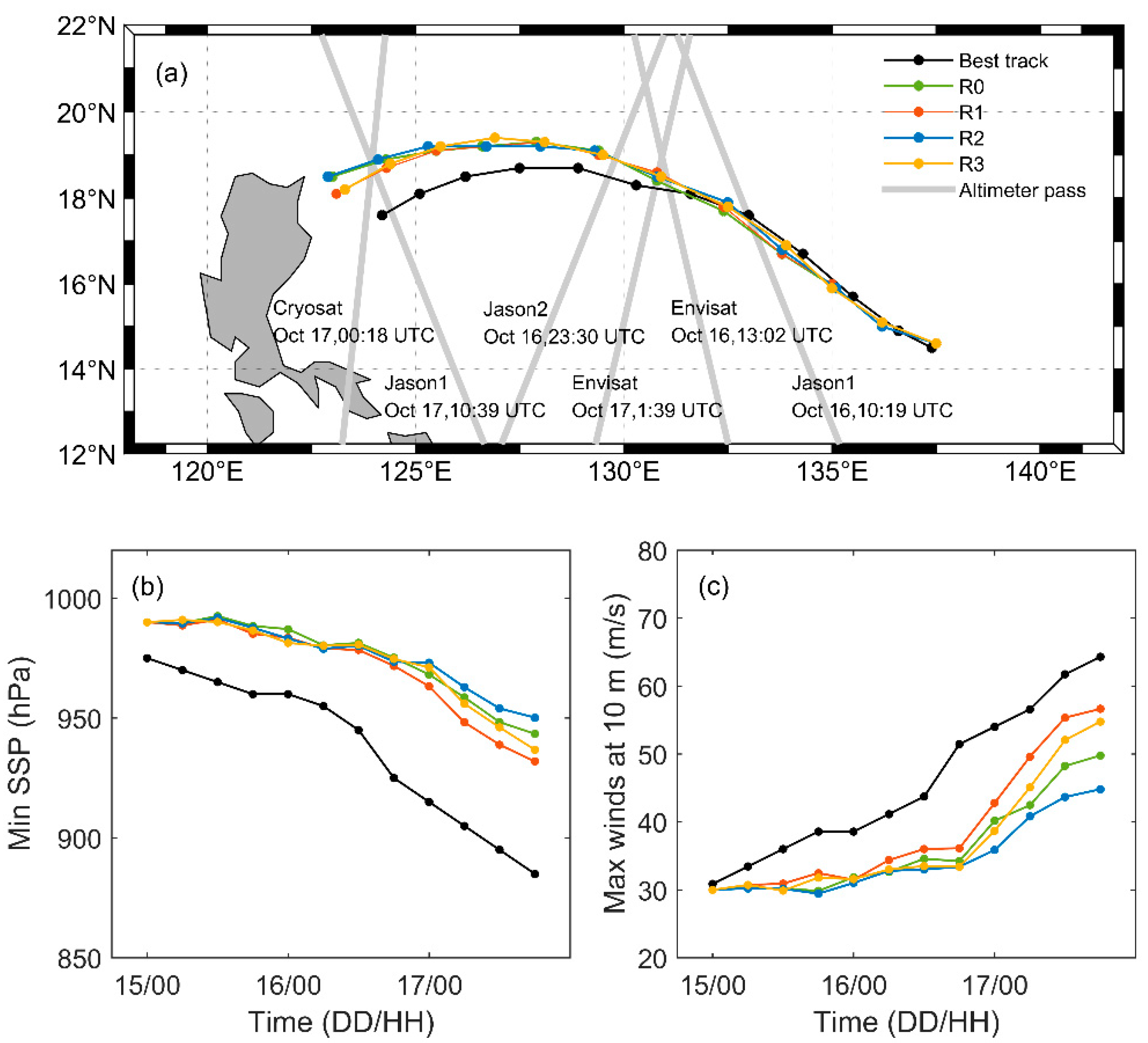
4.1. TC Track, Intensity, and Size
4.1.1. TC Track
4.1.2. TC Intensity
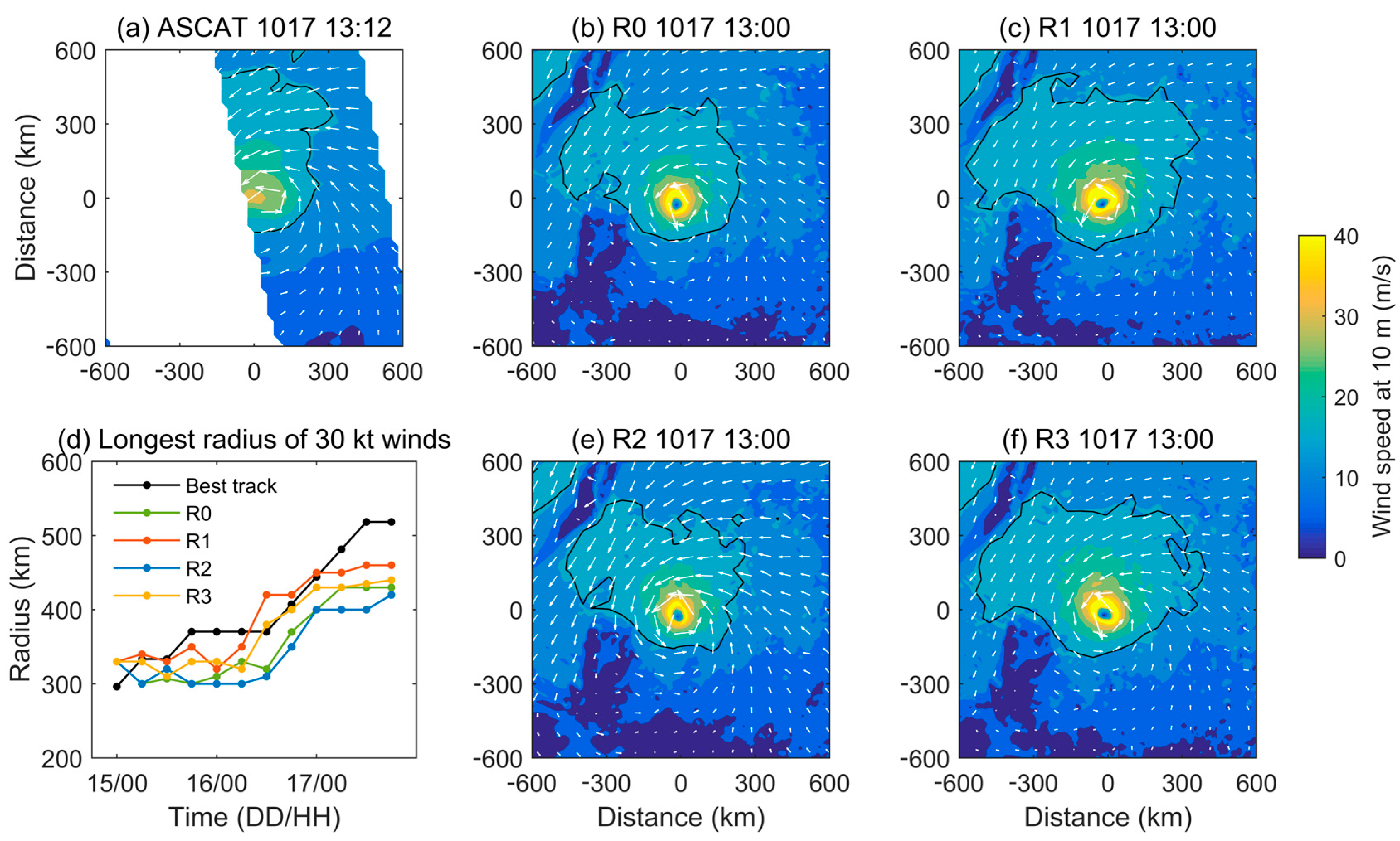
4.1.3. TC Size
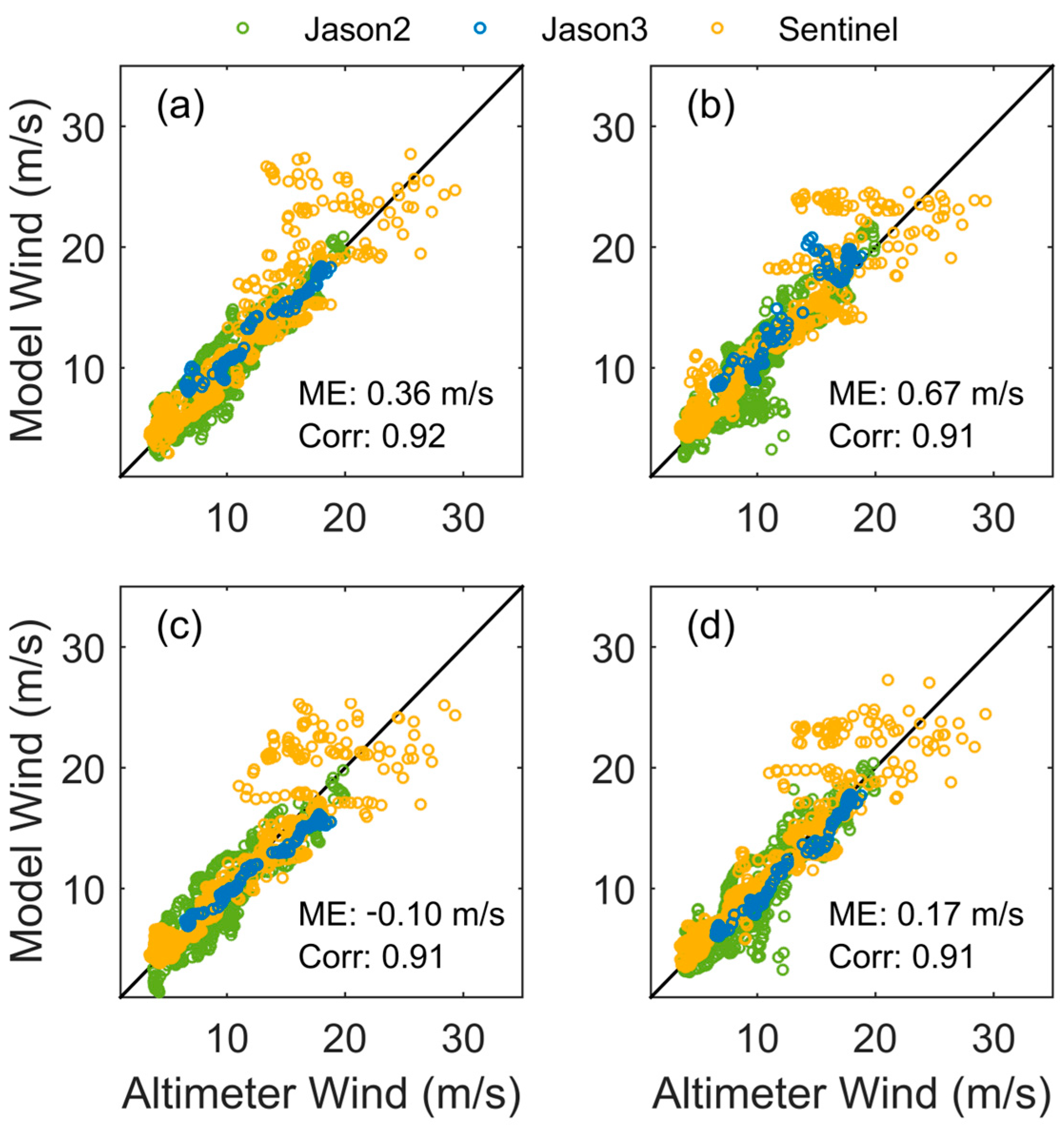
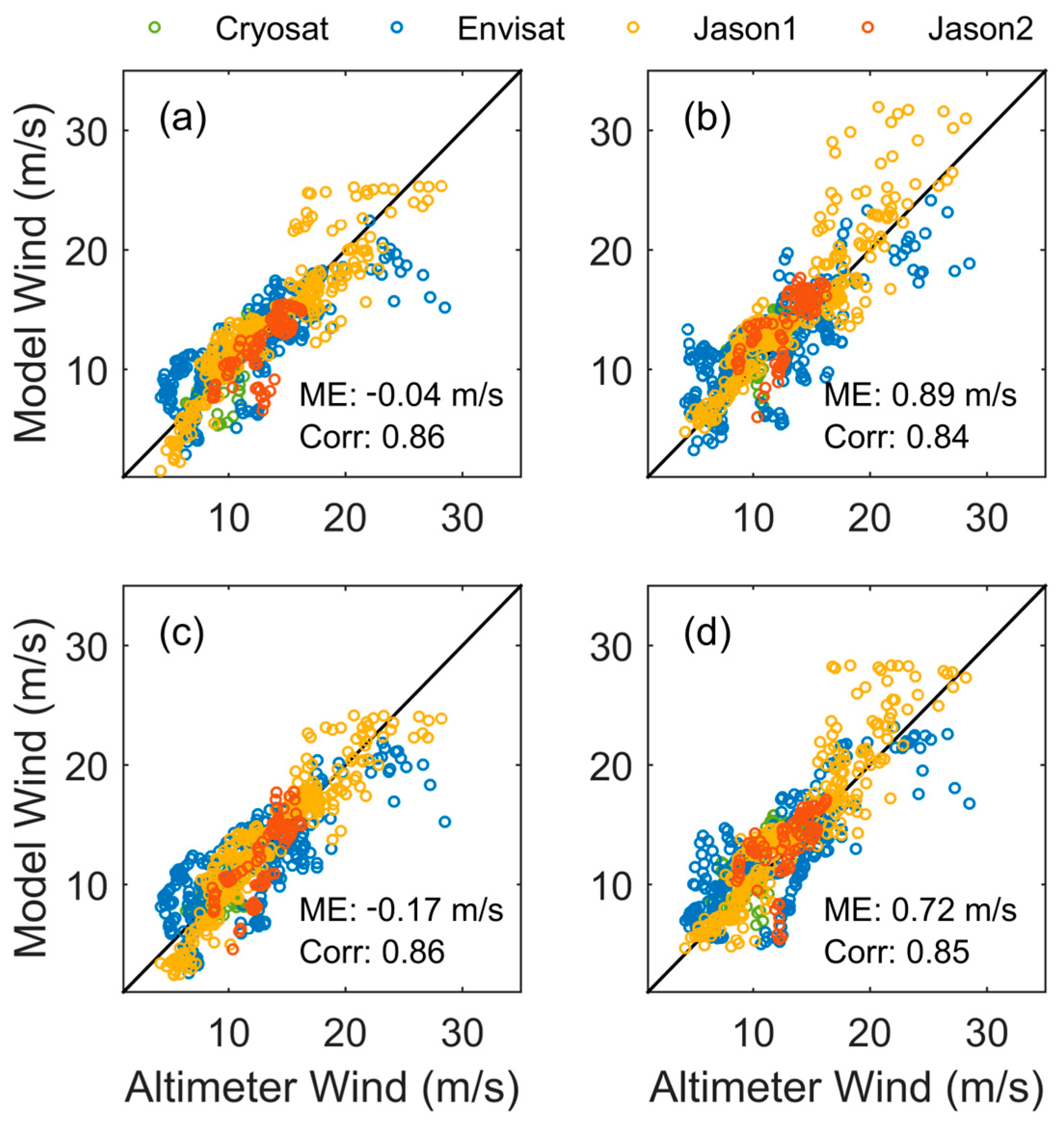
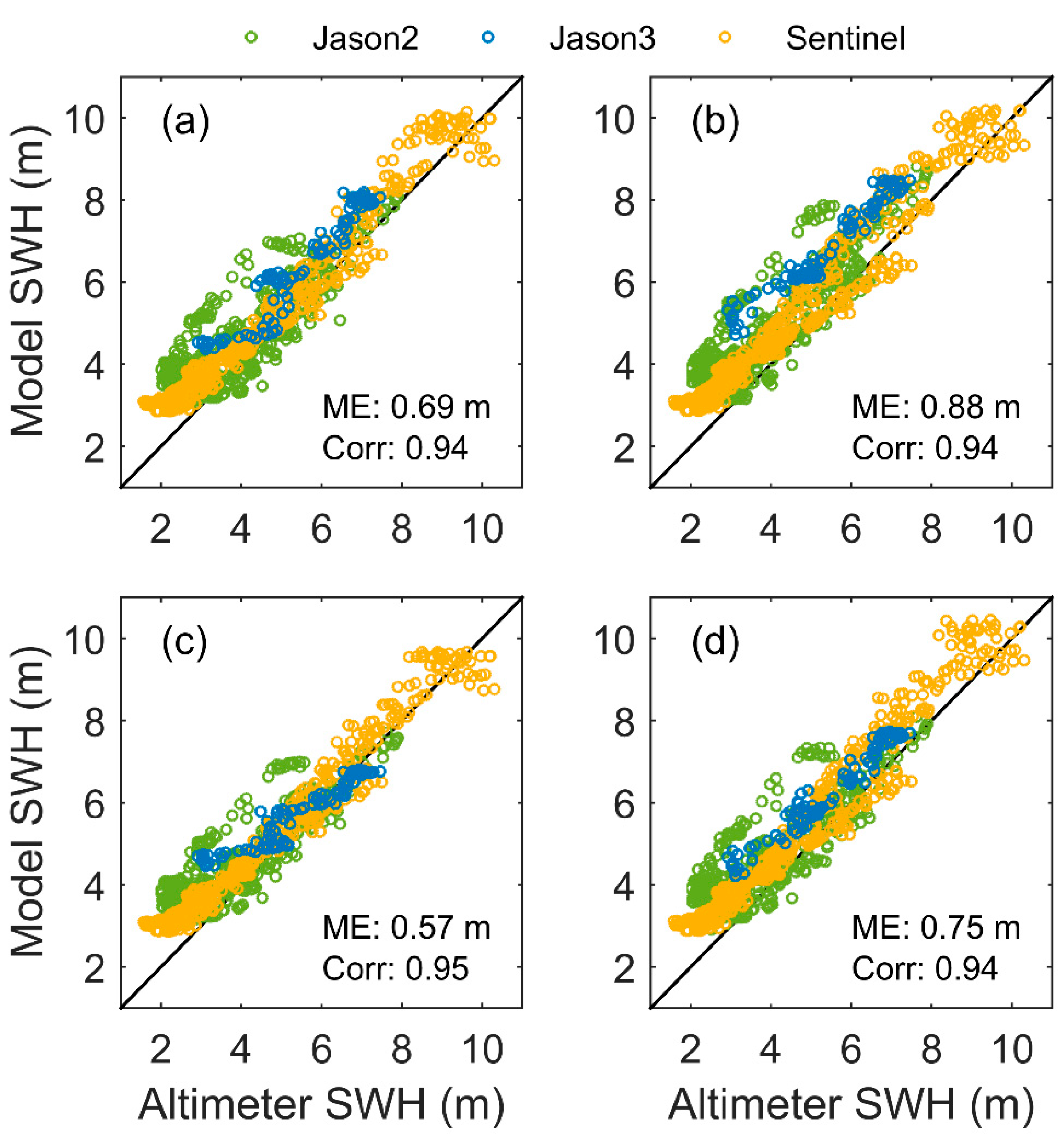
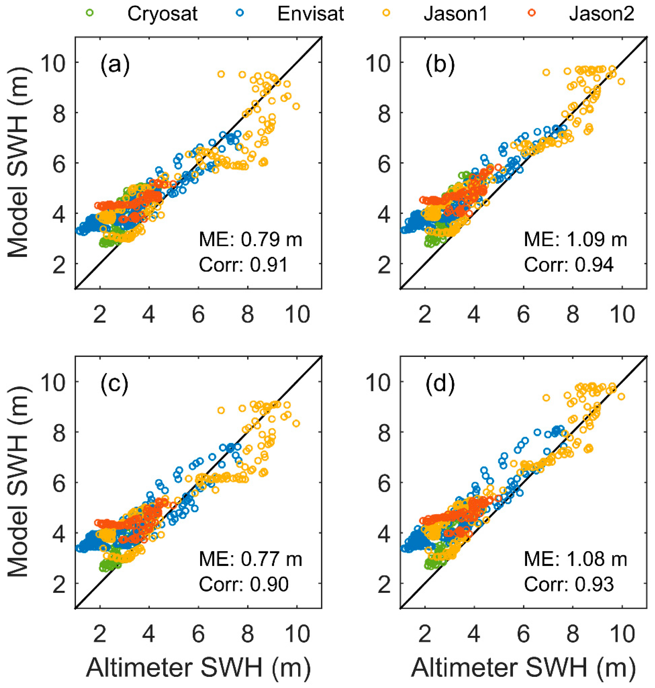
4.2. Validation for Surface Waves and Winds Using Altimeter Observations
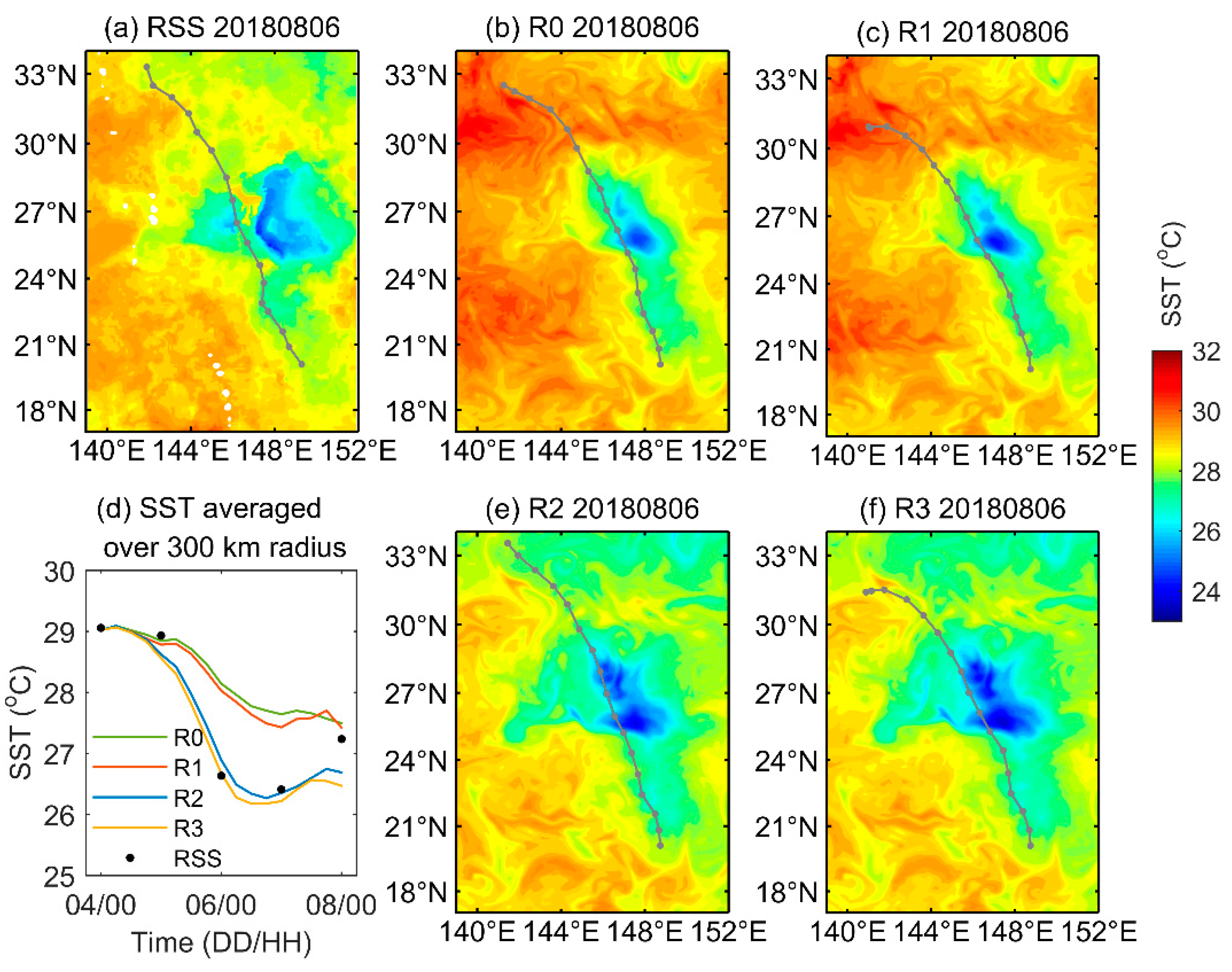
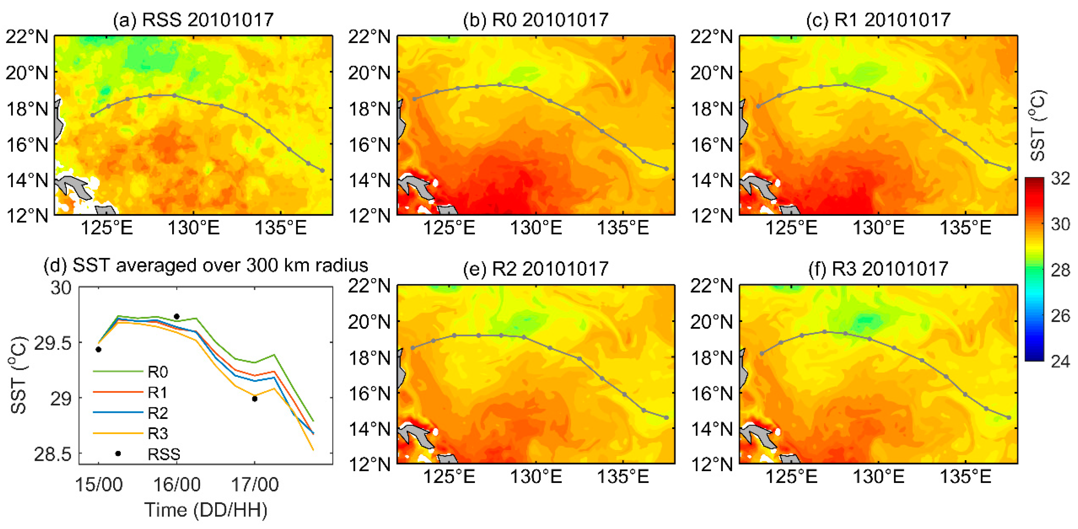
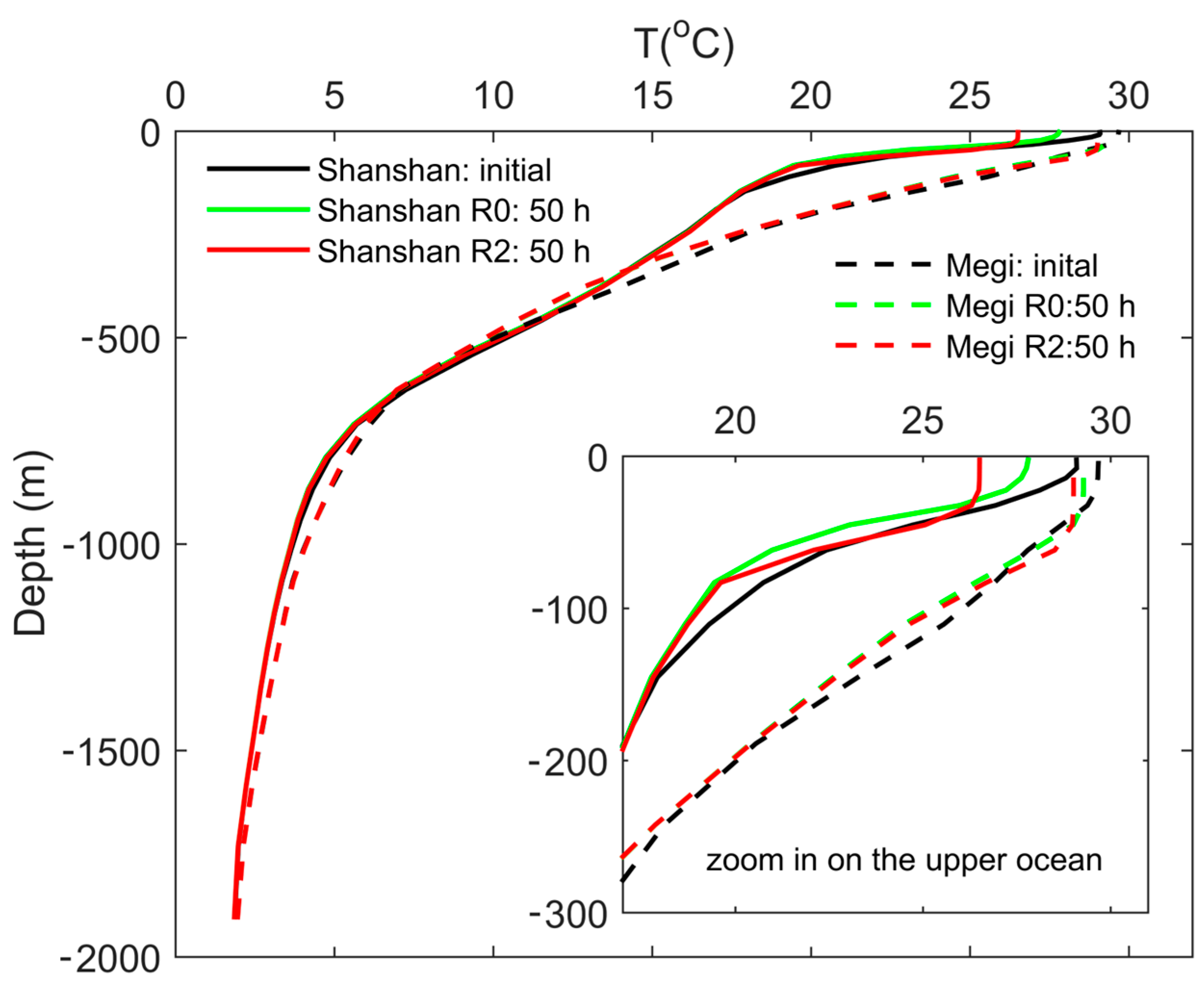
4.3. SST
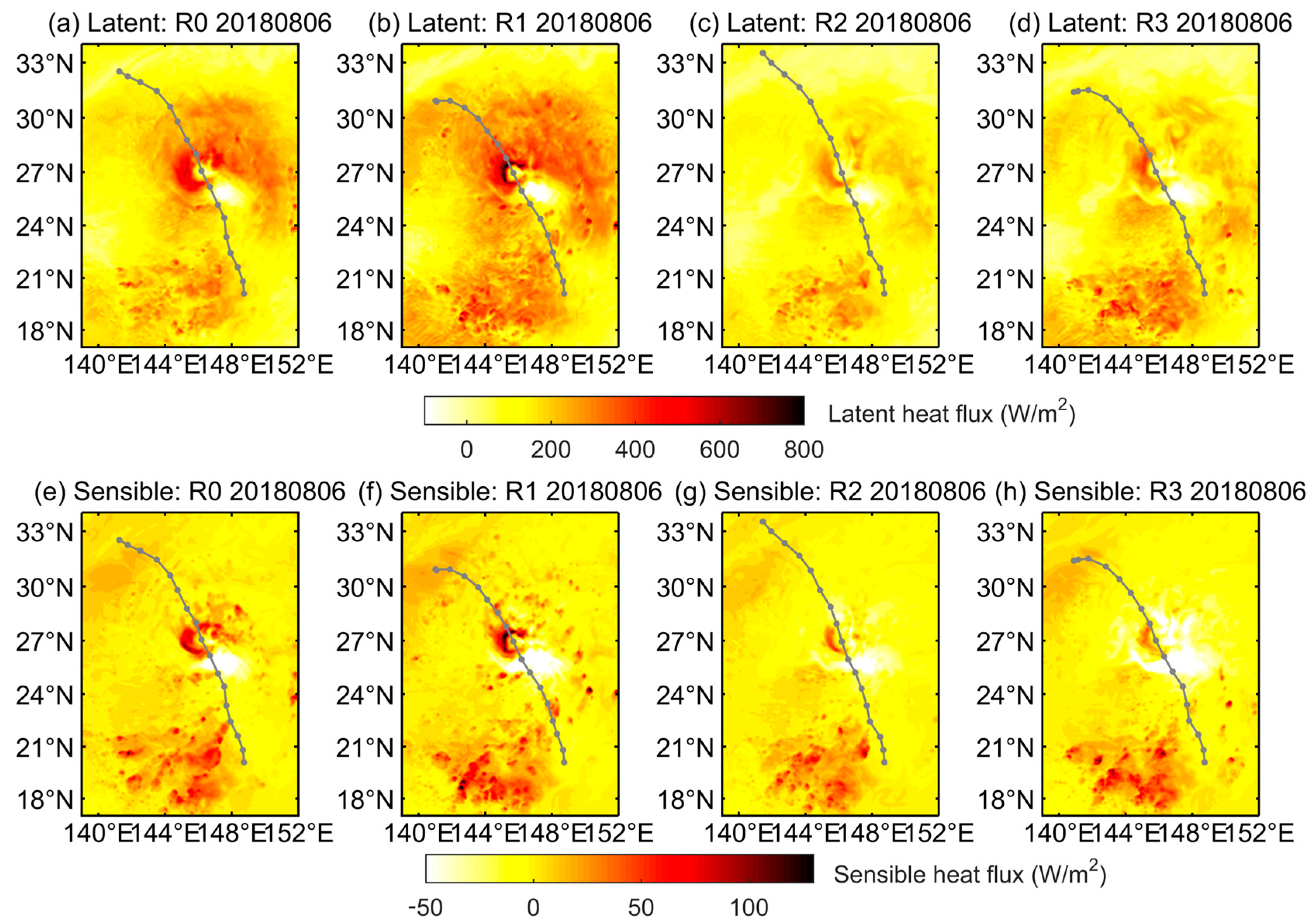
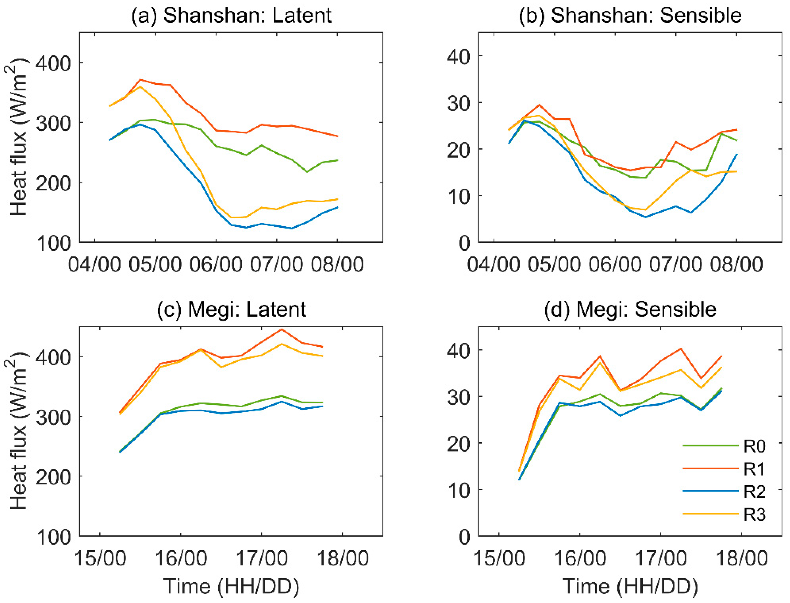
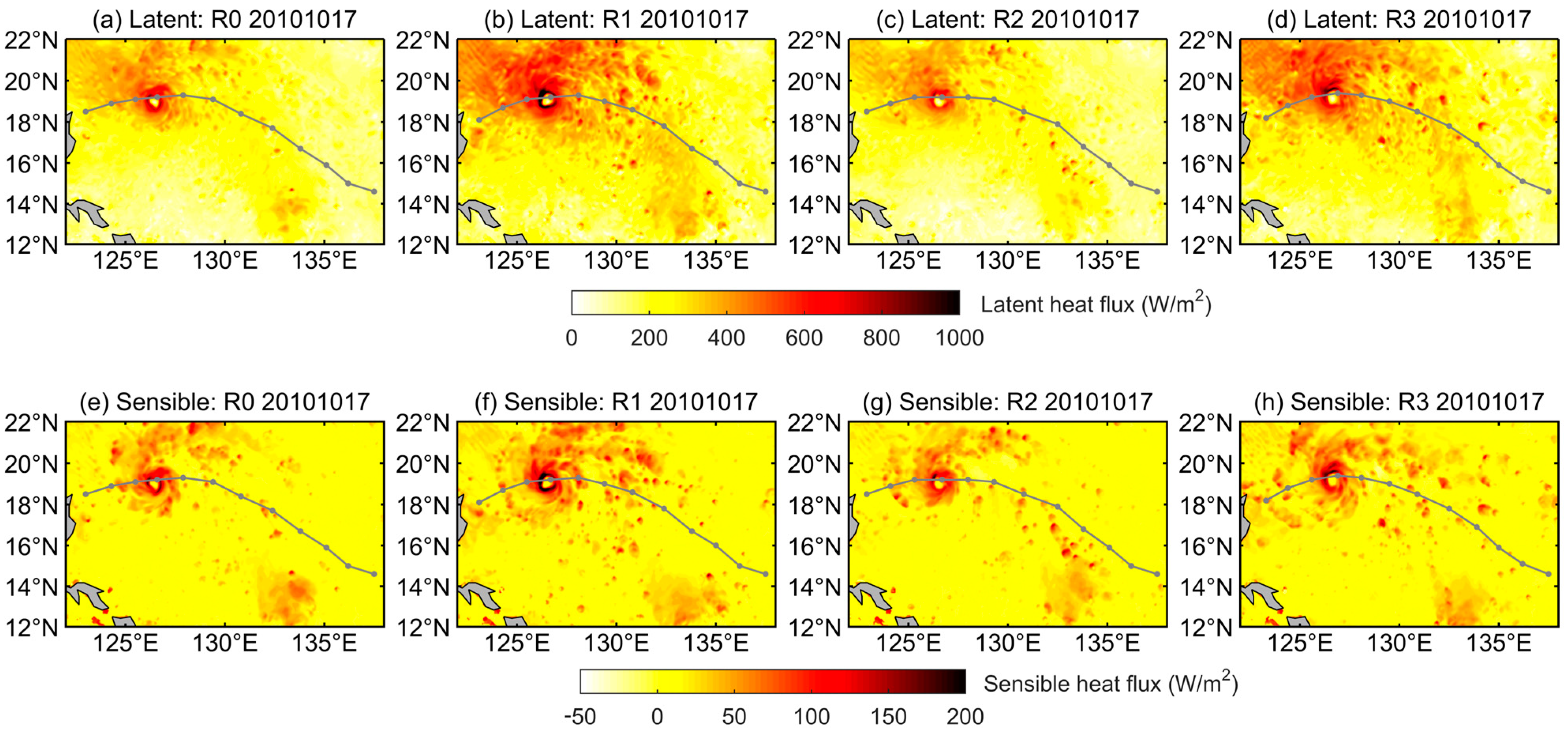
4.4. Heat Flux
5. Conclusions
Author Contributions
Funding
Data Availability Statement
Acknowledgments
Conflicts of Interest
Appendix A. Surface Exchange Coefficients in COARE 3.0
References
- Cangialosi, J.P.; Blake, E.; DeMaria, M.; Penny, A.; Latto, A.; Rappaport, E.; Tallapragada, V. Recent Progress in Tropical Cyclone Intensity Forecasting at the National Hurricane Center. Weather Forecast. 2020, 35, 1913–1922. [Google Scholar] [CrossRef]
- DeMaria, M.; Sampson, C.R.; Knaff, J.A.; Musgrave, K.D. Is Tropical Cyclone Intensity Guidance Improving? Bull. Am. Meteorol. Soc. 2014, 95, 387–398. [Google Scholar] [CrossRef] [Green Version]
- Emanuel, K.A.; Zhang, F. On the Predictability and Error Sources of Tropical Cyclone Intensity Forecasts. J. Atmos. Sci. 2016, 73, 3739–3747. [Google Scholar] [CrossRef] [Green Version]
- Chavas, D.R.; Knaff, J.A. A Simple Model for Predicting the Tropical Cyclone Radius of Maximum Wind from Outer Size. Weather Forecast. 2022, 37, 563–579. [Google Scholar] [CrossRef]
- Knaff, J.A.; Sampson, C.R. After a Decade Are Atlantic Tropical Cyclone Gale Force Wind Radii Forecasts Now Skillful? Weather Forecast. 2015, 30, 702–709. [Google Scholar] [CrossRef]
- Pun, I.F.; Knaff, J.A.; Sampson, C.R. Uncertainty of Tropical Cyclone Wind Radii on Sea Surface Temperature Cooling. J. Geophys. Res. Atmos. 2021, 126, e2021JD034857. [Google Scholar] [CrossRef]
- Sampson, C.R.; Goerss, J.S.; Knaff, J.A.; Strahl, B.R.; Fukada, E.M.; Serra, E.A. Tropical Cyclone Gale Wind Radii Estimates, Forecasts, and Error Forecasts for the Western North Pacific. Weather Forecast. 2018, 33, 1081–1092. [Google Scholar] [CrossRef]
- Emanuel, K.A. Thermodynamic control of hurricane intensity. Nature 1999, 401, 665–669. [Google Scholar] [CrossRef]
- Liu, B.; Liu, H.; Xie, L.; Guan, C.; Zhao, D. A Coupled Atmosphere-Wave-Ocean Modeling System: Simulation of the Intensity of an Idealized Tropical Cyclone. Mon. Weather Rev. 2011, 139, 132–152. [Google Scholar] [CrossRef]
- Zhang, W.; Zhao, D.; Zhu, D.; Li, J.; Guan, C.; Sun, J. A Numerical Investigation of the Effect of Wave-Induced Mixing on Tropical Cyclones Using a Coupled Ocean-Atmosphere-Wave Model. J. Geophys. Res. Atmos. 2022, 127, e2021JD036290. [Google Scholar] [CrossRef]
- Zhao, B.; Qiao, F.; Cavaleri, L.; Wang, G.; Bertotti, L.; Liu, L. Sensitivity of typhoon modeling to surface waves and rainfall. J. Geophys. Res. Oceans 2017, 122, 1702–1723. [Google Scholar] [CrossRef]
- Aijaz, S.; Ghantous, M.; Babanin, A.V.; Ginis, I.; Thomas, B.; Wake, G. Nonbreaking wave-induced mixing in upper ocean during tropical cyclones using coupled hurricane-ocean-wave modeling. J. Geophys. Res. Oceans 2017, 122, 3939–3963. [Google Scholar] [CrossRef] [Green Version]
- Reichl, B.G.; Wang, D.; Hara, T.; Ginis, I.; Kukulka, T. Langmuir Turbulence Parameterization in Tropical Cyclone Conditions. J. Phys. Oceanogr. 2016, 46, 863–886. [Google Scholar] [CrossRef]
- Toffoli, A.; McConochie, J.; Ghantous, M.; Loffredo, L.; Babanin, A.V. The effect of wave-induced turbulence on the ocean mixed layer during tropical cyclones: Field observations on the Australian North-West Shelf. J. Geophys. Res. Oceans 2012, 117, C00J24. [Google Scholar] [CrossRef] [Green Version]
- Zhang, X.; Chu, P.C.; Li, W.; Liu, C.; Zhang, L.; Shao, C.; Zhang, X.; Chao, G.; Zhao, Y. Impact of Langmuir Turbulence on the Thermal Response of the Ocean Surface Mixed Layer to Supertyphoon Haitang (2005). J. Phys. Oceanogr. 2018, 48, 1651–1674. [Google Scholar] [CrossRef]
- Komori, S.; Iwano, K.; Takagaki, N.; Onishi, R.; Kurose, R.; Takahashi, K.; Suzuki, N. Laboratory Measurements of Heat Transfer and Drag Coefficients at Extremely High Wind Speeds. J. Phys. Oceanogr. 2018, 48, 959–974. [Google Scholar] [CrossRef]
- Richter, D.H.; Stern, D.P. Evidence of spray-mediated air-sea enthalpy flux within tropical cyclones. Geophys. Res. Lett. 2014, 41, 2997–3003. [Google Scholar] [CrossRef]
- Sroka, S.; Emanuel, K. Sensitivity of Sea-Surface Enthalpy and Momentum Fluxes to Sea Spray Microphysics. J. Geophys. Res. Oceans 2022, 127, e2021JC017774. [Google Scholar] [CrossRef]
- Troitskaya, Y.; Sergeev, D.; Kandaurov, A.; Vdovin, M.; Zilitinkevich, S. The Effect of Foam on Waves and the Aerodynamic Roughness of the Water Surface at High Winds. J. Phys. Oceanogr. 2019, 49, 959–981. [Google Scholar] [CrossRef]
- Babanin, A.V. On a wave-induced turbulence and a wave-mixed upper ocean layer. Geophys. Rea. Lett. 2006, 33, L20605. [Google Scholar] [CrossRef]
- McWillams, J.C.; Sullivan, P.P.; Moeng, C.-H. Langmuir turbulence in the ocean. J. Fluid Mech. 1997, 334, 1–30. [Google Scholar] [CrossRef] [Green Version]
- Qiao, F.; Yuan, Y.; Yang, Y.; Zheng, Q.; Xia, C.; Ma, J. Wave-induced mixing in the upper ocean: Distribution and application to a global ocean circulation model. Geophys. Res. Lett. 2004, 31, L11303. [Google Scholar] [CrossRef]
- Kantha, L.H.; Clayson, C.A. An improved mixed layer model for geophysical applications. J. Geophys. Res. 1994, 99, 25235–25266. [Google Scholar] [CrossRef]
- Martin, P.J. Simulation of the mixed layer at OWS November and Papa with several models. J. Geophys. Res. 1985, 90, 903–916. [Google Scholar] [CrossRef]
- Green, B.W.; Zhang, F.Q. Impacts of Air-Sea Flux Parameterizations on the Intensity and Structure of Tropical Cyclones. Mon. Weather Rev. 2013, 141, 2308–2324. [Google Scholar] [CrossRef] [Green Version]
- Chen, S.S.; Price, J.F.; Zhao, W.; Donelan, M.A.; Walsh, E.J. The CBLAST-Hurricane Program and the Next-Generation Fully Coupled Atmosphere-Wave-Ocean Models for Hurricane Research and Prediction. Bull. Am. Meteorol. Soc. 2007, 88, 311–318. [Google Scholar] [CrossRef]
- Liu, B.; Guan, C.; Xie, L.; Zhao, D. An investigation of the effects of wave state and sea spray on an idealized typhoon using an air-sea coupled modeling system. Adv. Atmos. Sci. 2012, 29, 391–406. [Google Scholar] [CrossRef]
- Cavaleri, L.; Fox-Kemper, B.; Hemer, M. Wind Waves in the Coupled Climate System. Bull. Am. Meteorol. Soc. 2012, 93, 1651–1661. [Google Scholar] [CrossRef]
- Li, M.; Zahariev, K.; Garrett, C. Role of Langmuir circulation in the deepening of the ocean surface mixed layer. Science 1995, 270, 1955–1957. [Google Scholar] [CrossRef]
- Terray, E.A.; Donelan, M.A.; Agrawal, Y.C.; Drennan, W.M.; Kahma, K.K.; Williams, A.J.; Hwang, P.; Kitaigorodskii, S. Estimates of Kinetic Energy Dissipation under Breaking Waves. J. Phys. Oceanogr. 1996, 26, 792–804. [Google Scholar] [CrossRef]
- Babanin, A.V. Breaking and Dissipation of Ocean Surface Waves; Cambridge University Press: Cambridge, UK, 2011. [Google Scholar]
- Toba, Y.; Kawamura, H. Wind-wave coupled downward-bursting boundary layer (DBBL) beneath the sea surface. J. Oceanogr. 1996, 52, 409–419. [Google Scholar] [CrossRef]
- Burchard, H. Simulating the Wave-Enhanced Layer under Breaking Surface Waves with Two-Equation Turbulence Models. J. Phys. Oceanogr. 2001, 31, 3133–3145. [Google Scholar] [CrossRef]
- Craig, P.D.; Banner, M.L. Modeling Wave-Enhanced Turbulence in the Ocean Surface Layer. J. Phys. Oceanogr. 1994, 24, 2546–2559. [Google Scholar] [CrossRef]
- Huang, C.J.; Qiao, F.; Song, Z.; Ezer, T. Improving simulations of the upper ocean by inclusion of surface waves in the Mellor-Yamada turbulence scheme. J. Geophys. Res. 2011, 116, C01007. [Google Scholar] [CrossRef] [Green Version]
- Pleskachevsky, A.; Dobrynin, M.; Babanin, A.V.; Günther, H.; Stanev, E. Turbulent Mixing due to Surface Waves Indicated by Remote Sensing of Suspended Particulate Matter and Its Implementation into Coupled Modeling of Waves, Turbulence, and Circulation. J. Phys. Oceanogr. 2011, 41, 708–724. [Google Scholar] [CrossRef]
- Babanin, A.V.; Ganopolski, A.; Phillips, W.R.C. Wave-induced upper-ocean mixing in a climate model of intermediate complexity. Ocean Model. 2009, 29, 189–197. [Google Scholar] [CrossRef]
- Smith, J.A. Observed growth of Langmuir circulation. J. Geophys. Res. 1992, 97, 5651–5664. [Google Scholar] [CrossRef] [Green Version]
- Li, Q.; Reichl, B.G.; Fox-Kemper, B.; Adcroft, A.J.; Belcher, S.E.; Danabasoglu, G.; Grant, A.L.M.; Griffies, S.M.; Hallberg, R.; Hara, T.; et al. Comparing Ocean Surface Boundary Vertical Mixing Schemes Including Langmuir Turbulence. J. Adv. Model. Earth Syst. 2019, 11, 3545–3592. [Google Scholar] [CrossRef] [Green Version]
- Ghantous, M.; Babanin, A.V. Ocean mixing by wave orbital motion. Acta Phys. Slovaca 2014, 64, 1–56. [Google Scholar]
- Ghantous, M.; Babanin, A.V. One-dimensional modelling of upper ocean mixing by turbulence due to wave orbital motion. Nonlinear Process. Geophys. 2014, 21, 325–338. [Google Scholar] [CrossRef] [Green Version]
- Young, I.R.; Babanin, A.V.; Zieger, S. The Decay Rate of Ocean Swell Observed by Altimeter. J. Phys. Oceanogr. 2013, 43, 2322–2333. [Google Scholar] [CrossRef]
- Umlauf, L.; Burchard, H. A generic length-scale equation for geophysical. J. Mar. Res. 2003, 61, 235–265. [Google Scholar] [CrossRef]
- Warner, J.C.; Sherwood, C.R.; Arango, H.G.; Signell, R.P. Performance of four turbulence closure models implemented using a generic length scale method. Ocean Model. 2005, 8, 81–113. [Google Scholar] [CrossRef]
- Druzhinin, O.A.; Troitskaya, Y.I.; Zilitinkevich, S.S. The Study of Momentum, Mass, and Heat Transfer in a Droplet-Laden Turbulent Airflow Over a Waved Water Surface by Direct Numerical Simulation. J. Geophys. Res. Oceans 2018, 123, 8346–8365. [Google Scholar] [CrossRef] [Green Version]
- Rastigejev, Y.; Suslov, S.A.; Lin, Y.-L. Effect of Ocean Spray on Vertical Momentum Transport Under High-Wind Conditions. Bound. Layer Meteorol. 2011, 141, 1–20. [Google Scholar] [CrossRef] [Green Version]
- Troitskaya, Y.; Druzhinin, O.; Kozlov, D.; Zilitinkevich, S. The “Bag Breakup” Spume Droplet Generation Mechanism at High Winds. Part II: Contribution to Momentum and Enthalpy Transfer. J. Phys. Oceanogr. 2018, 48, 2189–2207. [Google Scholar] [CrossRef]
- Kudryavtsev, V.N.; Makin, V.K. Aerodynamic roughness of the sea surface at high winds. Bound. Layer Meteorol. 2007, 125, 289–303. [Google Scholar] [CrossRef]
- Troitskaya, Y.; Kandaurov, A.; Ermakova, O.; Kozlov, D.; Sergeev, D.; Zilitinkevich, S. Bag-breakup fragmentation as the dominant mechanism of sea-spray production in high winds. Sci. Rep. 2017, 7, 1614. [Google Scholar] [CrossRef] [Green Version]
- Powell, M.D.; Vickery, P.J.; Reinhold, T.A. Reduced drag coefficient for high wind speeds in tropical cyclones. Nature 2003, 422, 279–283. [Google Scholar] [CrossRef]
- Holthuijsen, L.H.; Powell, M.D.; Pietrzak, J.D. Wind and waves in extreme hurricanes. J. Geophys. Res. 2012, 117, C09003. [Google Scholar] [CrossRef] [Green Version]
- Donelan, M.A. On the decrease of the oceanic drag coefficient in high winds. J. Geophys. Res. Oceans 2018, 123, 1485–1501. [Google Scholar] [CrossRef]
- Bell, M.M.; Montgomery, M.T.; Emanuel, K.A. Air–Sea Enthalpy and Momentum Exchange at Major Hurricane Wind Speeds Observed during CBLAST. J. Atmos. Sci. 2012, 69, 3197–3222. [Google Scholar] [CrossRef]
- Takagaki, N.; Komori, S.; Suzuki, N.; Iwano, K.; Kuramoto, T.; Shimada, S.; Kurose, R.; Takahashi, K. Strong correlation between the drag coefficient and the shape of the wind sea spectrum over a broad range of wind speeds. Geophys. Res. Lett. 2012, 39, L23604. [Google Scholar] [CrossRef] [Green Version]
- Curcic, M.; Haus, B.K. Revised estimates of ocean surface drag in strong winds. Geophys. Res. Lett. 2020, 47, e2020GL087647. [Google Scholar] [CrossRef]
- Andreas, E.L.; Emanuel, K. Effects of Sea Spray on Tropical Cyclone Intensity. J. Atmos. Sci. 2001, 58, 3741–3751. [Google Scholar] [CrossRef]
- Peng, T.; Richter, D. Sea Spray and Its Feedback Effects: Assessing Bulk Algorithms of Air-Sea Heat Fluxes via Direct Numerical Simulations. J. Phys. Oceanogr. 2019, 49, 1403–1421. [Google Scholar] [CrossRef]
- Veron, F. Ocean Spray. Annu. Rev. Fluid Mech. 2015, 47, 507–538. [Google Scholar] [CrossRef]
- Korolev, V.S.; Petrichenko, S.A.; Pudov, V.D. Heat and moisture exchange between the ocean and atmosphere in tropical storms Tess and Skip. Sov. Meteor. Hydrol. 1990, 3, 92–94. [Google Scholar]
- Troitskaya, Y.; Sergeev, D.; Vdovin, M.; Kandaurov, A.; Ermakova, O.; Takagaki, N. A Laboratory Study of the Effect of Surface Waves on Heat and Momentum Transfer at High Wind Speeds. J. Geophys. Res. Oceans 2020, 125, e2020JC016276. [Google Scholar] [CrossRef]
- Fairall, C.W.; Bradley, E.F.; Hare, J.E.; Grachev, A.A.; Edson, J.B. Bulk Parameterization of Air-Sea Fluxes_ Updates and Verification for the COARE Algorithm. J. Clim. 2003, 16, 571–591. [Google Scholar] [CrossRef]
- Andreas, E.L.; Mahrt, L.; Vickers, D. An improved bulk air-sea surface flux algorithm, including spray-mediated transfer. Q. J. R. Meteorol. Soc. 2014, 141, 642–654. [Google Scholar] [CrossRef]
- Fairall, C.W.; Kepert, J.D.; Holland, G.J. The effect of sea spray on surface energy transports over the ocean. Glob. Atmos. Ocean Syst. 1994, 2, 121–142. [Google Scholar]
- Zhang, L.; Zhang, X.; Perrie, W.; Guan, C.; Dan, B.; Sun, C.; Wu, X.; Liu, K.; Li, D. Impact of Sea Spray and Sea Surface Roughness on the Upper Ocean Response to Super Typhoon Haitang (2005). J. Phys. Oceanogr. 2021, 51, 1929–1945. [Google Scholar] [CrossRef]
- Andreas, E.L. A review of the sea spray generation function for the open ocean. In Atmosphere-Ocean Interactions; WIT: Southhampton, UK, 2002; Volume 1, pp. 1–46. [Google Scholar]
- Warner, J.C.; Armstrong, B.; He, R.; Zambon, J.B. Development of a Coupled Ocean-Atmosphere-Wave-Sediment Transport (COAWST) Modeling System. Ocean Model. 2010, 35, 230–244. [Google Scholar] [CrossRef] [Green Version]
- Skamarock, W.C.; Klemp, J.B.; Dudhia, J.; Gill, D.O.; Barker, D.; Duda, M.G.; Huang, X.-Y.; Wang, W.; Powers, J.G. A Description of the Advanced Research WRF Version 3. NCAR Tech. Note NCAR/TN-475+STR. 2008; 113p. Available online: https://opensky.ucar.edu/islandora/object/technotes%3A500/datastream/PDF/view (accessed on 2 June 2022).
- Booij, N.R.R.C.; Ris, R.C.; Holthuijsen, L.H. A third-generation wave model for coastal regions: 1. Model description and validation. J. Geophys. Res. Oceans 1999, 104, 7649–7666. [Google Scholar] [CrossRef] [Green Version]
- Warner, J.C.; Sherwood, C.R.; Signen, R.P.; Harris, C.K.; Arango, H.G. Development of a three-dimensional, regional, coupled wave, current, and sediment-transport model. Comput. Geosci. 2008, 34, 1284–1306. [Google Scholar] [CrossRef]
- The WAVEWATCH III Development Group (WW3DG). User Manual and System Documentation of WAVEWATCH III TM version 6.07, NOAA/NWS/NCEP/MMAB Technical Note 333. 2019. Available online: https://www.weather.gov/sti/coastalact_ww3 (accessed on 2 June 2022).
- Nakanishi, M.; Niino, H. An Improved Mellor-Yamada Level-3 Model: Its Numerical Stability and Application to a Regional Prediction of Advection Fog. Bound. Layer Meteorol. 2006, 119, 397–407. [Google Scholar] [CrossRef]
- Mlawer, E.J.; Taubman, S.J.; Brown, P.D.; Iacono, M.J.; Clough, S.A. Radiative transfer for inhomogeneous atmospheres: RRTM, avalidated correlated-k model for the longwave. J. Geophys. Res. 1997, 102, 16–663. [Google Scholar] [CrossRef] [Green Version]
- Dudhia, J. Numerical study of convection observed during the winter monsoon experiment using a mesoscale two-dimensional model. J. Atmos. Sci. 1989, 46, 3077–3107. [Google Scholar] [CrossRef]
- Lin, Y.-L.; Farley, R.D.; Orville, H.D. Bulk parameterization of the snow field in a cloud model. J. Clim. Appl. Meteorol. 1983, 22, 1065–1092. [Google Scholar] [CrossRef]
- Chen, F.; Dudhia, J. Coupling an advanced land surface-hydrology model with the Penn State-NCAR MM5 modeling system. Part I: Model implementation and sensitivity. Mon. Weather Rev. 2001, 129, 569–585. [Google Scholar] [CrossRef]
- Olabarrieta, M.; Warner, J.C.; Armstrong, B.; Zambon, J.B.; He, R. Ocean-atmosphere dynamics during Hurricane Ida and Nor’Ida: An application of the coupled ocean-atmosphere-wave-sediment transport (COAWST) modeling system. Ocean Model. 2012, 43–44, 112–137. [Google Scholar] [CrossRef] [Green Version]
- Kumar, N.; Voulgaris, G.; Warner, J.C.; Olabarrieta, M. Implementation of the vortex force formalism in the coupled ocean-atmosphere wave-sediment transport (COAWST) modeling system for inner shelf and surf zone applications. Ocean Model. 2012, 47, 65–95. [Google Scholar] [CrossRef]
- Zambon, J.B.; He, R.; Warner, J.C. Tropical to extratropical: Marine environmental changes associated with Superstorm Sandy prior to its landfall. Geophys. Res. Lett. 2014, 41, 8935–8943. [Google Scholar] [CrossRef] [Green Version]
- Zambon, J.B.; He, R.; Warner, J.C.; Hegermiller, C.A. Impact of SST and Surface Waves on Hurricane Florence (2018): A Coupled Modeling Investigation. Weather Forecast. 2021, 36, 1713–1734. [Google Scholar] [CrossRef]
- Hasselmann, K.; Barnett, T.; Bouws, E.; Carlson, H.; Cartwright, D.; Enke, K.; Ewing, J.A.; Gienapp, H.; Hasselmann, D.E.; Kruseman, P.; et al. Measurements of wind-wave growth and swell decay during the Joint north sea wave project (JONSWAP). Ergänzung Zur Dtsch. Hydrogr. Zeitschrift. 1973, 12, 1–95. [Google Scholar]
- Ribal, A.; Young, I.R. 33 years of globally calibrated wave height and wind speed data based on altimeter observations. Sci. Data 2019, 6, 1–15. [Google Scholar] [CrossRef] [Green Version]
- Bender, M.A.; Ginis, I. Real-Case Simulations of Hurricane Ocean Interaction Using A High-Resolution Coupled Model: Effects on Hurricane Intensity. Mon. Weather Rev. 2000, 128, 917–946. [Google Scholar] [CrossRef]
- Meissner, T.; Wentz, F.J. Wind vector retrievals under rain with passive satellite microwave radiometers. IEEE Trans. Geosci. Remote 2009, 47, 3065–3083. [Google Scholar] [CrossRef]
- Young, I.R.; Sanina, E.; Babanin, A.V. Calibration and Cross Validation of a Global Wind and Wave Database of Altimeter, Radiometer, and Scatterometer Measurements. J. Atmos. Ocean. Technol. 2017, 34, 1285–1306. [Google Scholar] [CrossRef]
- Tamizi, A.; Young, I.R.; Ribal, A.; Alves, J.-H. Global scatterometer observations of the structure of tropical cyclone wind fields. Mon. Weather Rev. 2020, 148, 4673–4692. [Google Scholar] [CrossRef]
- Ribal, A.; Tamizi, A.; Young, I.R. Calibration of Scatterometer Wind Speed under Hurricane Conditions. J. Phys. Oceanogr. 2021, 38, 1859–1870. [Google Scholar] [CrossRef]
- Wu, R.; Zhang, H.; Chen, D.; Li, C.; Lin, J. Impact of Typhoon Kalmaegi (2014) on the South China Sea: Simulations using a fully coupled atmosphere-ocean-wave model. Ocean Model. 2018, 131, 132–151. [Google Scholar] [CrossRef]
- Zhou, X.; Hara, T.; Ginis, I.; D’Asaro, E.; Hsu, J.; Reichl, B.G. Drag Coefficient and Its Sea State Dependence under Tropical Cyclones. J. Phys. Oceanogr. 2022, 52, 1447–1470. [Google Scholar] [CrossRef]
- Zhang, W. Dataset of “Effects of Surface Wave-Induced Mixing and Wave-Affected Exchange Coefficients on Tropical Cyclones”. [Dataset] Figshare. 2022. Available online: https://figshare.com/articles/dataset/Dataset_of_Effects_of_surface_waves_on_tropical_cyclones_/20449518/1 (accessed on 1 October 2022).
- National Centers for Environmental Prediction/National Weather Service/NOAA/U.S. Department of Commerce. NCEP FNL operational model global tropospheric analyses, continuing from July 1999 [Dataset]. In Research Data Archive at the National Center for Atmospheric Research; Computational and Information Systems Laboratory: Boulder, CO, USA, 2000. [Google Scholar] [CrossRef]
- Cummings, J.A. Operational multivariate ocean data assimilation. Q. J. R. Meteorol. Soc. 2005, 131, 3583–3604. [Google Scholar] [CrossRef] [Green Version]
- Ricciardulli, L.; Wentz, F.J. Remote Sensing Systems ASCAT C-2015 Daily Ocean Vector Winds on 0.25 Deg Grid, Version 02.1 [Dataset]; Remote Sensing Systems: Santa Rosa, CA, USA, 2016; Available online: https://www.remss.com (accessed on 2 June 2022).
- Wentz, F.J.; Ricciardulli, L.; Gentemann, C.; Meissner, T.; Hilburn, K.A.; Scott, J. Remote Sensing Systems Coriolis WindSat Daily Environmental Suite on 0.25 Deg Grid, Version 7.0.1 [Dataset]; Remote Sensing Systems: Santa Rosa, CA, USA, 2013; Available online: https://www.remss.com/missions/windsat (accessed on 2 June 2022).
- IMOS. IMOS—SRS Surface Waves Sub-Facility—Altimeter Wave/Wind [Dataset]. Australian Ocean Data Network. 2010–2018. Available online: https://portal.aodn.org.au/search (accessed on 2 June 2022).
- Smith, S.D. Coefficients for sea surface wind stress, heat flux, and wind profiles as a function of wind speed and temperature. J. Geophys. Res. 1988, 93, 15467–15472. [Google Scholar] [CrossRef]
- Charnock, H. Wind stress on a water surface. Q. J. R. Meteorol. Soc. 1955, 81, 639–640. [Google Scholar] [CrossRef]


| Expts. | Parameterizations for the Surface Exchange Coefficients | Wave-Induced Mixing |
|---|---|---|
| R0 | COARE 3.0 | No |
| R1 | Equations (4) and (5) | No |
| R2 | COARE 3.0 | Equation (1) |
| R3 | Equations (4) and (5) | Equation (1) |
| Shanshan | |||||||
| Expt. | Track | Min SSP | Max Winds at 10 m | Longest Radius of 30 kt | |||
| Error (km) | Error (hPa) | Relative Error (%) | Error (m/s) | Relative Error (%) | Error (km) | Relative Error (%) | |
| R0 | 52.7 | −6.7 | 0.75 | 0.6 | 4.5 | −49.1 | 8.8 |
| R1 | 111.0 | −16.2 | 1.67 | 6.8 | 19.0 | −5.8 | 3.4 |
| R2 | 47.7 | 0.2 | 0.45 | −3.1 | 8.7 | −103.2 | 18.6 |
| R3 | 91.6 | −4.2 | 0.64 | −0.8 | 5.2 | −90.2 | 16.2 |
| Megi | |||||||
| Expt. | Track | Min SSP | Max Winds at 10 m | Longest Radius of 30 kt | |||
| Error (km) | Error (hPa) | Relative Error (%) | Error (m/s) | Relative Error (%) | Error (km) | Relative Error (%) | |
| R0 | 106.2 | 42.9 | 4.7 | −11.8 | 23.3 | −59.1 | 13.8 |
| R1 | 98.6 | 37.2 | 4.0 | −8.4 | 17.0 | −19.1 | 7.9 |
| R2 | 110.1 | 44.3 | 4.8 | −13.9 | 27.1 | −74.7 | 17.4 |
| R3 | 93.0 | 40.9 | 4.4 | −10.7 | 21.4 | −39.7 | 9.4 |
Disclaimer/Publisher’s Note: The statements, opinions and data contained in all publications are solely those of the individual author(s) and contributor(s) and not of MDPI and/or the editor(s). MDPI and/or the editor(s) disclaim responsibility for any injury to people or property resulting from any ideas, methods, instructions or products referred to in the content. |
© 2023 by the authors. Licensee MDPI, Basel, Switzerland. This article is an open access article distributed under the terms and conditions of the Creative Commons Attribution (CC BY) license (https://creativecommons.org/licenses/by/4.0/).
Share and Cite
Zhang, W.; Zhang, J.; Liu, Q.; Sun, J.; Li, R.; Guan, C. Effects of Surface Wave-Induced Mixing and Wave-Affected Exchange Coefficients on Tropical Cyclones. Remote Sens. 2023, 15, 1594. https://doi.org/10.3390/rs15061594
Zhang W, Zhang J, Liu Q, Sun J, Li R, Guan C. Effects of Surface Wave-Induced Mixing and Wave-Affected Exchange Coefficients on Tropical Cyclones. Remote Sensing. 2023; 15(6):1594. https://doi.org/10.3390/rs15061594
Chicago/Turabian StyleZhang, Wenqing, Jialin Zhang, Qingxiang Liu, Jian Sun, Rui Li, and Changlong Guan. 2023. "Effects of Surface Wave-Induced Mixing and Wave-Affected Exchange Coefficients on Tropical Cyclones" Remote Sensing 15, no. 6: 1594. https://doi.org/10.3390/rs15061594