Article

A Principal Component Analysis Methodology of Oil Spill Detection and Monitoring Using Satellite Remote Sensing Sensors

by
Niyazi Arslan
1,
Meysam Majidi Nezhad
2,*,
Azim Heydari
3,4,
Davide Astiaso Garcia
5 and
Georgios Sylaios
6
1
Department of Mining Engineering, Cukurova University, Adana 01330, Turkey
2
Department of Sustainable Energy Systems, Mälardalen University, SE 72123 Västerås, Sweden
3
Department of Astronautics, Electrical and Energy Engineering (DIAEE), Sapienza University of Rome, 00184 Rome, Italy
4
Department of Energy Management and Optimization, Institute of Science and High Technology and Environmental Sciences, Graduate University of Advanced Technology, Kerman 7631133131, Iran
5
Department of Planning, Design, Technology of Architecture, Sapienza University of Rome, 00185 Rome, Italy
6
Laboratory of Ecological Engineering and Technology, Department of Environmental Engineering, Democritus University of Thrace, 67100 Xanthi, Greece
*
Author to whom correspondence should be addressed.
Remote Sens. 2023, 15(5), 1460; https://doi.org/10.3390/rs15051460
Submission received: 22 February 2023 / Revised: 1 March 2023 / Accepted: 2 March 2023 / Published: 5 March 2023
(This article belongs to the Special Issue Feature Paper Special Issue on Ocean Remote Sensing - Part 2)

Abstract

:
Monitoring, assessing, and measuring oil spills is essential in protecting the marine environment and in efforts to clean oil spills. One of the most recent oil spills happened near Port Fourchon, Louisiana, caused by Hurricane Ida (Category 4), that had a wind speed of 240 km/h. In this regard, Earth Observation (EO) Satellite Remote Sensing (SRS) images can effectively highlight oil spills in marine areas as a “fast and no-cost” technique. However, clouds and the sea surface spectral signature complicate the interpretation of oil spill areas in the optical images. In this study, Principal Component Analysis (PCA) has been applied of Landsat-8 and Sentinel-2 SRS images to improve information from the optical sensor bands. The PCA produces an output unrelated to the main bands, making it easier to distinguish oil spills from clouds and seawater due to the spectral diversity between oil, clouds, and the seawater surface. Then, an additional step has been applied to highlight the oil spill area using PCAs with different band combinations. Furthermore, Sentinel-1 (SAR), Sentinel-2 (optical), and Landsat-8 (optical) SRS images have been analyzed with cross-sections to suppress the “look-alike” effect of marine oil spill areas. Finally, mean and high-pass filters were used for Land Surface Temperature (LST) SRS images estimated from the Landsat thermal band. The results show that the seawater value is about −17.5 db and the oil spill area shows a value between −22.5 db and −25 db; the Landsat 8 satellites thermal band 10, depicting contrast at some areas for oil spill, can be determined by the 3 × 3 and 5 × 5 Kernel High pass and the 3 × 3 Mean filter. The results demonstrate that the SRS images should be used together to improve oil spill detection studies results.

1. Introduction

Environmental pollution monitoring has recently become one of the scientific community’s areas of central interest [1]. The degree of environmental pollution is correlated with human society’s population growth, and this human population requires materials and resources such as water, food, mines, and oil to maintain their lives [2,3]. Therefore, governments and companies are increasing their efforts to find new sources of oil and gas in remote and deep marine areas to meet these needs. Oil production and transportation involves risk, including oil spills, especially in exploration and maritime transport [4]. Earth Observation-based (EO) Satellite Remote Sensing (SRS) data can detect environmental pollutants in large marine areas [5], including oil spills [6,7]. The occurrence of oil pollution directly impacts marine mammals, marine grasses, coral reefs, and fish populations and leads to economic damage to fish farms, tourism activities areas, and marine ecosystems [8,9].
Oil spills have short-term, medium-term, and long-term effects requiring timely and accurate marine area policies [10]. In this regard, “fast and no-cost” techniques and methods updated based on new knowledge can be very effective in monitoring, diagnosis, measurement, and forecasting. These techniques can provide the best possible information in the shortest time to politicians and researchers. For example, a report compiled and updated by the International Tanker Owners Pollution Federation (ITOPF) shows that large-scale oil spill disasters (rather than oil spills) decreased at sea and in oceans between 1970 and 2021 [11]. However, it should be noted that the ITOPF report only contains information from published sources and ship owners, meaning that many illegal fuel discharges and small accidents may have been overlooked. One reason for this could be the dramatic growth of high-precision marine technology, greater sensitivity to the marine environment, and appropriate policies and investments to increase maritime safety and reduce oil spills.
The amount of oil released from the oil tanker accidents at sea in 2021 was approximately 10,000 tons; this can be considered significant. The total amount of oil released into the seas and oceans will be almost 1.7 billion tons by 2021 and 2020 [11]. The biggest oil spill in the last ten years was the SANCHI [12] ship accident in the China Sea on 6 January 2018. More than 136,000 tons of oil were released at sea, and all the ship occupants were killed [12]. Although the rate of oil spills has decreased sharply in recent years, it should be remembered that the assessment and detection of oil spills is the first fundamental phase, “phase one”, required to reduce the oil spill risk. This phase must be continuously developed and improved. Finally, it should not be forgotten that other causes of oil spills, such as non-shipping, pipeline leaks, offshore oil exploration, industrial activities, and natural oil seeps, can significantly increase the rate of global oil spills in marine areas [11].
SRS images can use different reflections between marine water and the types and thicknesses of related oil spills for oil monitoring [13]. Oil reflection properties depend on many factors, including oil class and thickness [14]. These parameters mean its wavelength is different from seawater [15]. The multi-sensor satellite imagery used to monitor environmental pollution, including oil spills, has become an efficient and standard method. However, EO SRS data output can be improved by integrating satellite data for oil spill detection, assessment, monitoring, and reporting [16]. Traditionally, data from reconnaissance aircraft and research vessels are commonly used to measure oil spills in marine areas. However, using traditional tools to identify oil spills can be costly and time-consuming in marine areas.
In this regard, oil spill monitoring using SRS data with optical sensors [17], such as Landsat-8 and Sentinel-2, and radar sensors [18], such as the Sentinel-1 (SAR) satellite, has been widely used [19]. There are also polarimetric SAR studies with different statistical and classification approaches for oil spills [4,5]. Many different types of research on oil spill modelling and analysis have been conducted in seas and oceans, including the Mediterranean Sea [20,21], Adriatic Sea [22], North Sea [23,24], Lebanon shoreline [25], South Aegean (Crete) [26], Persian Gulf [27], and the Indian Ocean [28]. However, oil spill monitoring using the SRS technique has some drawbacks, as bio-genic films, low wind speed, internal waves, ship wakes, grease ice, algae, shallow water, and rain cells cause the “look-alike” pattern, resulting in the misinterpretation of the results [29].
For example, the capabilities of optical sensors including Sentinel-2 and Landsat-8 SRS data can vary concerning optical conditions, film thickness, and oil and marine optical properties. In addition, the optical sensor capabilities depend on cloud and fog coverage of images considered for processing optical images. The results of various studies show that to achieve the best results in the oil spill investigation, active and passive SRS should be used together to increase reliability [30]. In addition, these sensors have different bands with spatial, temporal, radiometric, and bandwidth resolutions that cover a wide range. Used together, each benefit of the SRS sensors can be used to better detect oil slicks.
As mentioned above, even though the optical images have some drawbacks, they show satisfactory spatial resolution, which helps detect micro-oil spills; this overcomes a significant issue in the identification general problem. Colossal oil spills that occurred in connection with the BP Deepwater Horizon accident are significantly different to micro-oil spills, which are usually much more frequent, especially in coastal zones, and cannot be detected if poor spatial resolution is in place. Caruso et al. [5] mentioned using different polarimetric SAR satellite image during the BP Deepwater Horizon accident. They stated that this system could be efficiently used in oil spill detection studies across a wide area using different SAR imaging modes. The degree of wind speed is a restrictive factor for SAR studies.
Wang et al. [31] state that detecting oil spill marine pollution based on changes in lighting conditions of visible images is very efficient. Based on this, thermal infrared images are not affected by changes in illumination, and so can be used to determine the oil spill area. They study introduced a new method to determine areas with oil spills using thermal infrared fusion and visible images. First, their study extracted areas with oil spills using thermal infrared image processing help. Next, they used Principal Component Analysis (PCA) fusion between visible and thermal infrared images and background information to detect oil spills. This method examines the areas with natural oil spills using the pixel area calculation method. Their experimental results state that the method has an average error of about 2.78%. In addition, the proposed method can achieve better evaluation and objective index results than other methods.
El-Rahman et al. [32] used four hyperspectral image classification approaches: Support Vector Machine (SVM), parallelism, Minimum Distance (MD), and Binary Encoding (BE). Four classification approaches are applied after pre-processing in two studied areas, including spatial and spectral subsets and atmospheric correction. Applying the PCA method is used to remove redundant data, reduce a large amount of information, and reduce the processing time. The research results show that the SVM, MD, and BE approaches provide higher classification accuracy than the parallel approach. Liu et al. [33] developed a method for oil spill detection with laser remote sensing using time-resolved fluorescence in connection with parallel factor analysis of the oil spill dataset. They used PCA as a comparative method. Their research shows that the PCA method effectively classifies large oil spills. Almulihi et al. [34] used PCA to reduce extracted feature dimensions in the oil spill investigation dataset.
This study analyzes the Port Fourchon oil spills using SRS sensors, including Sentinel-1, Sentinel-2, and Landsat-8. First, the PCA is applied to Landsat-8 and Sentinel-2 SRS images to improve the optical sensor band information. The PCA produces an output unrelated to the main bands, making it easier to distinguish oil spills from clouds and seawater due to the unclear spectral characteristics of oil, clouds, the sea, and ocean in some pixels. Second, an additional step is applied to highlight the oil spill area using PCAs taking different band combinations. Furthermore, Sentinel-1 (SAR), Sentinel-2 (optical), and Landsat-8 (optical) images are analyzed with cross-sections to suppress the look-alike” effect of marine oil areas. The progress of the oil spill should be addressed carefully to define the disaster extent. Each sensor has advantages and disadvantages in showing oil spill areas. The information combination from the different sensors is a prerequisite for a reliable interpretation of the oil spill area. SRS image processing techniques, such as PCA and filtering methods, have been applied to demonstrate the oil spill progress precisely. This study combines the EO SRS information, focusing on different image processing techniques, to demonstrate the oil spill progress. It should be noted that the EO SRS information data use and its analysis with “Fast and no-cost” techniques and methods can significantly speed up data analysis and the decision-making processes of stakeholders and marine environmental project policymakers.

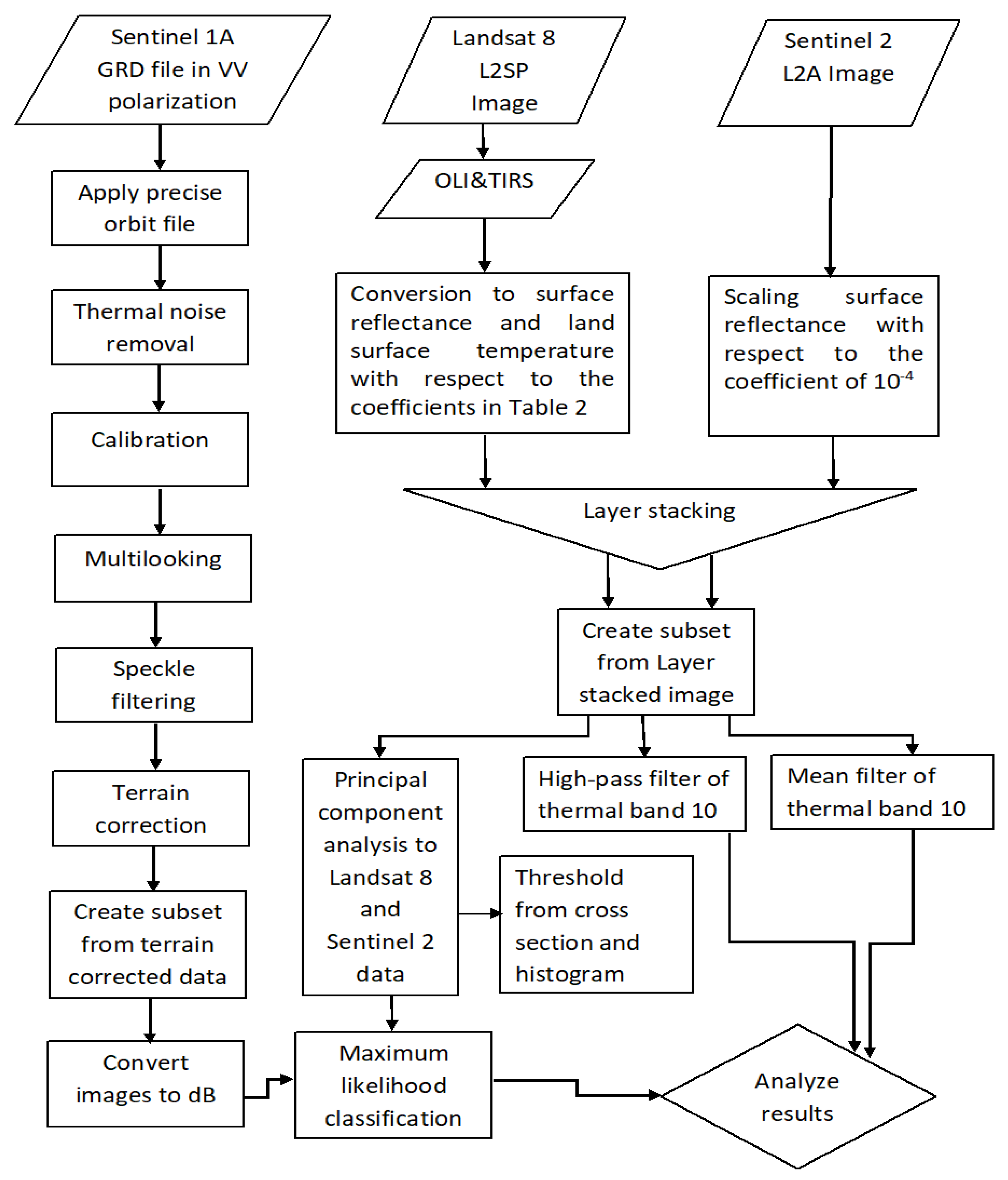
2. Materials and Methods
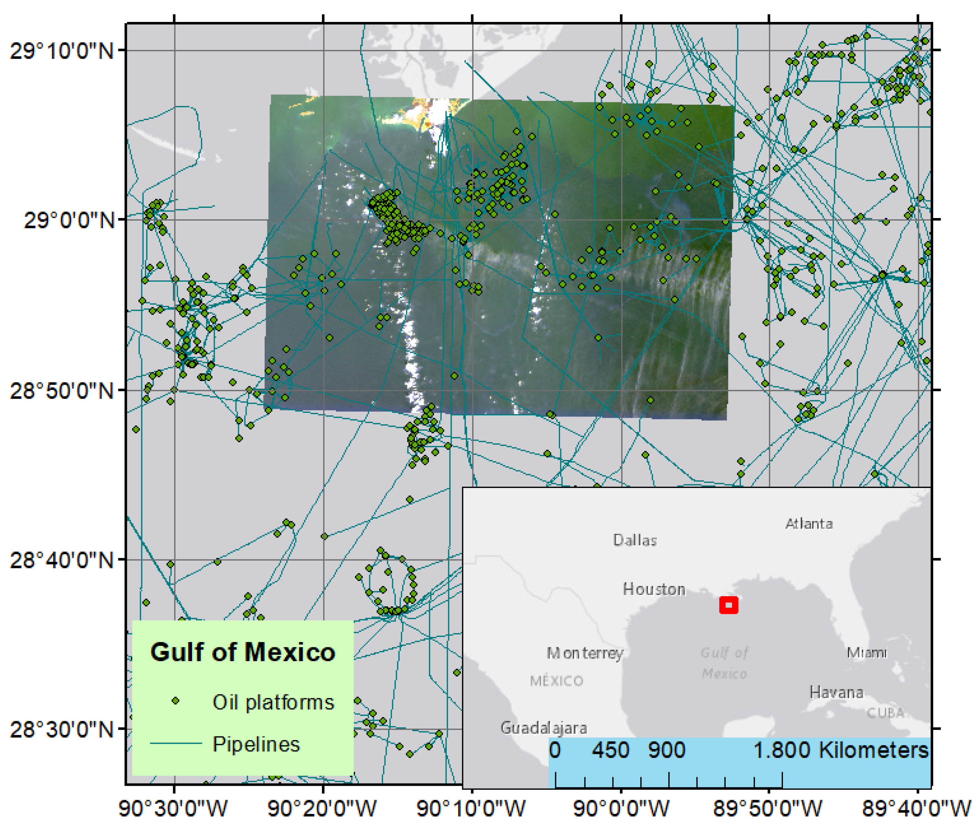
The methodological approach consists of the following five phases: (1) Case study; (2) SRS data; (3) Maximum Likelihood (ML) classification; (4) The PCA; and (5) Analyzing the oil spill event using SRS filters.

2.1. Case Study

The oil spill event occurred around Port Fourchon due to Hurricane Ida. Hurricane Ida was a category four hurricane with a wind speed of 240 (km/h), which began on 30 August 2021. This hurricane accounted for the oil spill in the Gulf of Mexico around Port Fourchon, Louisiana. U.S. Coast Guard and federal agencies coordinated the studies on finding the oil spill source. Divers found some clues about the oil source under the Gulf of Mexico ocean floor as pipelines in shallow water were used to transport the oil. They found ruptured 30 cm diameter pipelines in different locations, resulting in oil spills across the marine area. The amount of oil released amount into the water is unclear. This oil spill event was also validated using aerial images from an airplane flight and SRS.
The National Oceanic and Atmospheric Administration (NOAA) presented aerial images area showing thick oil (dark) surrounded by a rainbow sheen on 2 September 2021. It was stated that a miles-long brown and black oil spill was located 3 km to the south of Port Fourchon, Louisiana, and that it did not affect the shoreline. The area generally includes old pipelines, abandoned platforms, and plugged wells alongside the new platforms and plants [35,36,37,38]. Figure 1 shows the study area.

2.2. SRS Data

Sentinel-1, Landsat 8, and Sentinel-2 SRS data were used to define the oil spill region (Table 1). Sentinel-1 is a C-band SAR instrument with a central frequency of 5.405 GHz and a wavelength of ~5.55 cm. It has a single polarization (HH or VV) and dual-polarization (HH + HV or VV + VH) with 10 m resolution. Sentinel-1A and Sentinel-1B satellites are in the same orbit and have six days’ temporal resolution [39,40,41]. The Sentinel-1 data is in a multi-looked IW GRD product and projected to the ground range using an Earth ellipsoid model [41].
Table 2 shows OLI and TIRS bands of the Landsat-8 satellite with the wavelength range, units, Multiplicative Scale Factor (MSF), Additive Scale Factor (ASF), and resolution. This study uses Landsat-8 Collection 2 T1 collection category (L2SP) product. The data are in 30-m spatial resolution, WGS84 ellipsoid, WGS84 datum, and Universal Transverse Mercator (UTM) projection of UTM Zone 15 [42].
Sentinel-2 Level-2A data show the Bottom-Of-Atmosphere (BOA) reflectance in the UTM projection of WGS84 Ellipsoid. Table 3 represents the Sentinel-2 band specification.
Sentinel-1, Sentinel-2, and Landsat-8 data should be preprocessed before applying image processing techniques. In the first stage, Sentinel Application Platform (SNAP) software is used to process Sentinel-1 Level-1 Interferometric Wide Swath (IW) Ground Range Detected (GRD) images for the generation of geocoded, calibrated (slope normalized), multi looked, despeckled sigma0_VV product for VV polarization. The SAR data preprocessing steps are provided in Figure 2 [30].
In the second stage, Landsat-8 data, given in Digital Numbers (DN), should be converted to surface reflectance and Land Surface Temperature (LST). Again, Equation (1) is used with the MSF and ASF values to restore the DNs to surface reflectance and LST values for the related band utilized in Table 2. In Equation (1) subscript i refers to the band number.
S i = M S F i D N i + A S F i
As the Sentinel-2 Level-2A data show the BOA reflectance in the UTM projection of WGS84, there is no need for further processing, except for scaling surface reflectance concerning the coefficient of 10−4.

2.3. Maximum Likelihood (ML) Classification

ML classification is a method of clustering pixels for the defined classes. The pixels for the clusters are primarily accumulated at the raster data scatter plot center. If the distribution of the pixels for a given class is expected, we can apply the rules for normal distribution probability. The probability distribution for the specific class can be written as follows:
P x ω i = 2 π N / 2 C i 0.5 e x p 1 / 2 x m i T C i 1 x m i
where x is the spectral vector, N is the spectral vector dimension, m i is the class mean i, and C i is the class covariance i. These two values define class distribution computed from the available training pixels (class signature). After class signatures are estimated for each category from the training data set, the class for a pixel can be estimated by comparing the class probabilities (conditional probability) corresponding to the highest chance. As we choose the pixel class with the ML, the method is mentioned as ML classification [43].

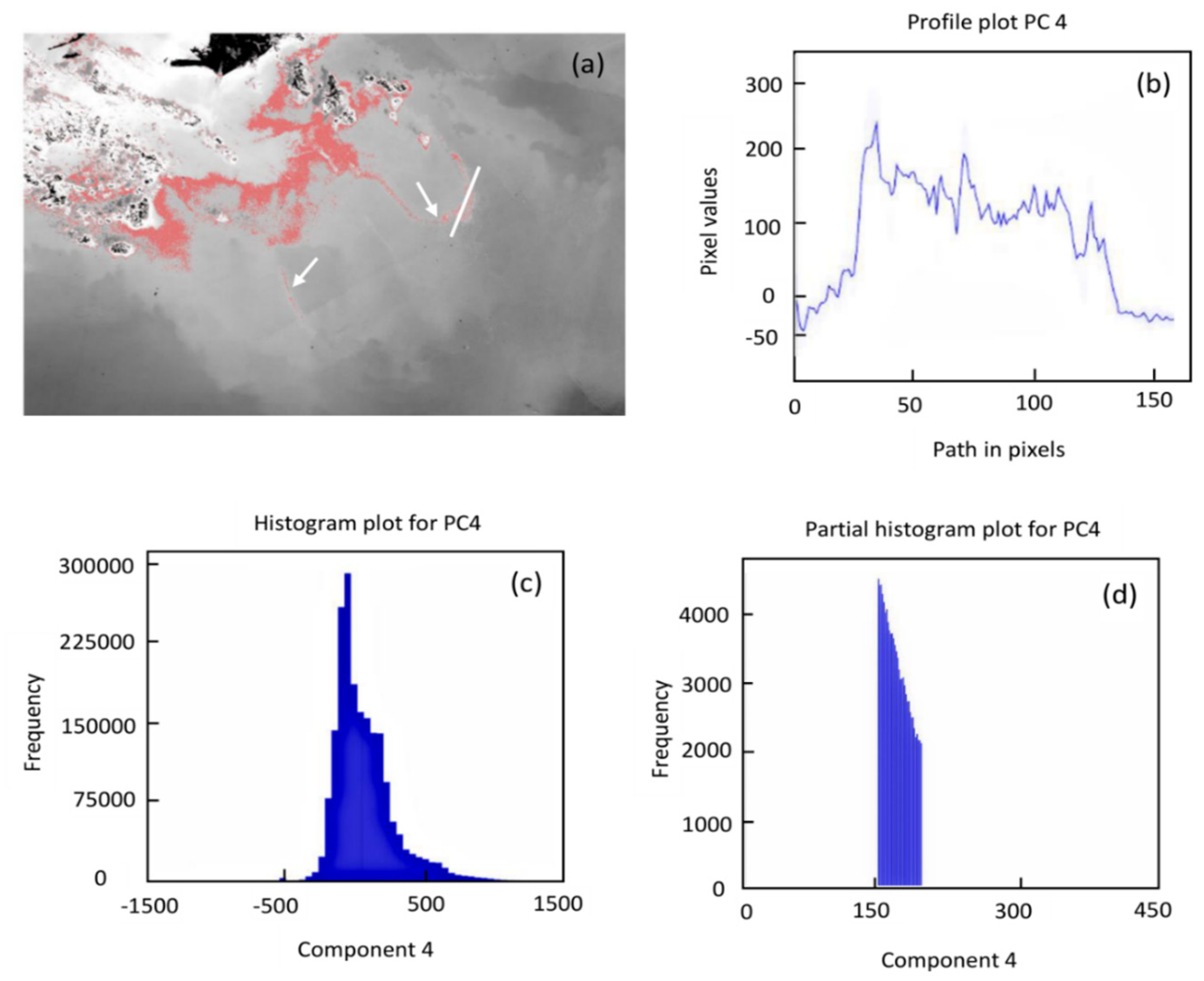
2.4. Principal Component Analysis (PCA)

There are several feature extraction methods, including PCA, Minimum Noise Fraction (MNF), independent component analysis (ICA), and Autoencoder, that can be used for dimension reduction of the proposed image [44,45,46]. These methods can be categorized, concerning the applied approach, as linear or nonlinear and Gaussian or non-Guassian distribution. PCA is a linear transformation, whereas autoencoder is a nonlinear transformation neural network method for reducing data dimension using a decoder and encoder. It recursively minimizes its noise fraction using the same eigenvalues and eigenvectors as PCA for the MNF [47]. If the image bands distribution is not Gaussian, non-Gaussian methods, namely ICA, can be applied. The ICA can be assumed as a linear representation of non-Gaussian data [48]. Ibarrola-Ulzurrun et al. [46] studied the PCA, MNF, and ICA with different components and represented the image classification with a support vector machine using a different parameter, area of interest, and component. They found that the overall accuracy is over 96.5% for MNF and PCA, and about 95% for ICA at 20 components. They stated that the MNF results are slightly better than the PCA results. Chen et al. [49] applied band reduction methods, such as MNF and PCA, to MASTER airborne imagery analysis of forest fires. They stated that the PCA-based model provides better results than MNF because of the latter’s deficiency in separating similar reflectance values from different features. It can be said that the selected methodologies and performance depend on the data distribution, the image noise level, the band number, the classification parameters used for accuracy assessment, and the interest selected area.
In this study, the PCA method used because of its applicability ease with remote sensing software and the satisfactory accuracy for feature extraction. PCA is a dimension reduction technique, and the pixels from SRS data bands are converted to PCA using a maximum variance. These PCA are constructed from original bands in a different direction. The result is uncorrelated orthogonal bands that include the most valuable information after conversion. The component’s number can be equal to or less than the original bands. Most information is included in the first two bands, followed by the remainder with minor details. Each PCA band has different information at the grayscale level.
Therefore, the PCA band images show various minor and significant details after the transformation. The bands should be selected concerning the gradients in the image for the PCA band components’ exciting feature regardless of the number by visual inspection. In order to separate features such as oil spills, threshold values for the gradients can be defined concerning the changes in the pixel values utilized from histogram and profile plots.
The SRS image can be given by the matrix of:
X k = x 1 x 2 x n
where k shows the number of bands and x n is the image vector of nth bands. To reduce the dimension of the bands, covariance matrix for eigenvalues should be calculated as follows:
C b , b = σ 1 , 1 σ 1 , n σ n , 1 σ n , n
The variance-covariance elements of the matrix of Cb,b can be computed using Equation (5):
σ i , j = 1 N 1 p = 1 N D N p , i μ i D N p , j μ j
where D N p , i is a digital number of a pixel p in the band i,   D N p , j is a DN of a pixel p in the band j, and μ i and μ j is the mean of DN for the bands i and j, respectively. The eigenvalues can be calculated by:
det C λ I = 0
with the covariance matrix C and diagonal identity matrix I. The principal components can be estimated by:
Y k = y 1 y 2 y n = w 1 , 1 w 1 , n w n , 1 w n , n x 1 x 2 x n
In this equation Y is the vector of PCA and W is the transformation matrix. The transformation matrix can be obtained from the estimated eigenvectors [50].

2.5. Filters

A high-pass filter removes the low-frequency component of an image, thereby enhancing the high-frequency component. High-pass filters are mentioned as edge enhancement filters aimed at image edge detection. Mean filters are low pass filters that reduce the image’s noise. It removes Gaussian noise. This study uses 3 × 3 and 5 × 5 kernel High-pass and 5 × 5 kernel mean filters to find the gradients and reduce noise in the Landsat 8 thermal band 10 [51].

3. Results and Discussion

The optical and radar SRS data are used to analyze the Hurricane Ida oil spill event in the Gulf of Mexico. The information is selected from all available images that cover the oil spill period with low cloud coverage. Figure 2 shows the methodology flowchart used in the oil spill area analysis.

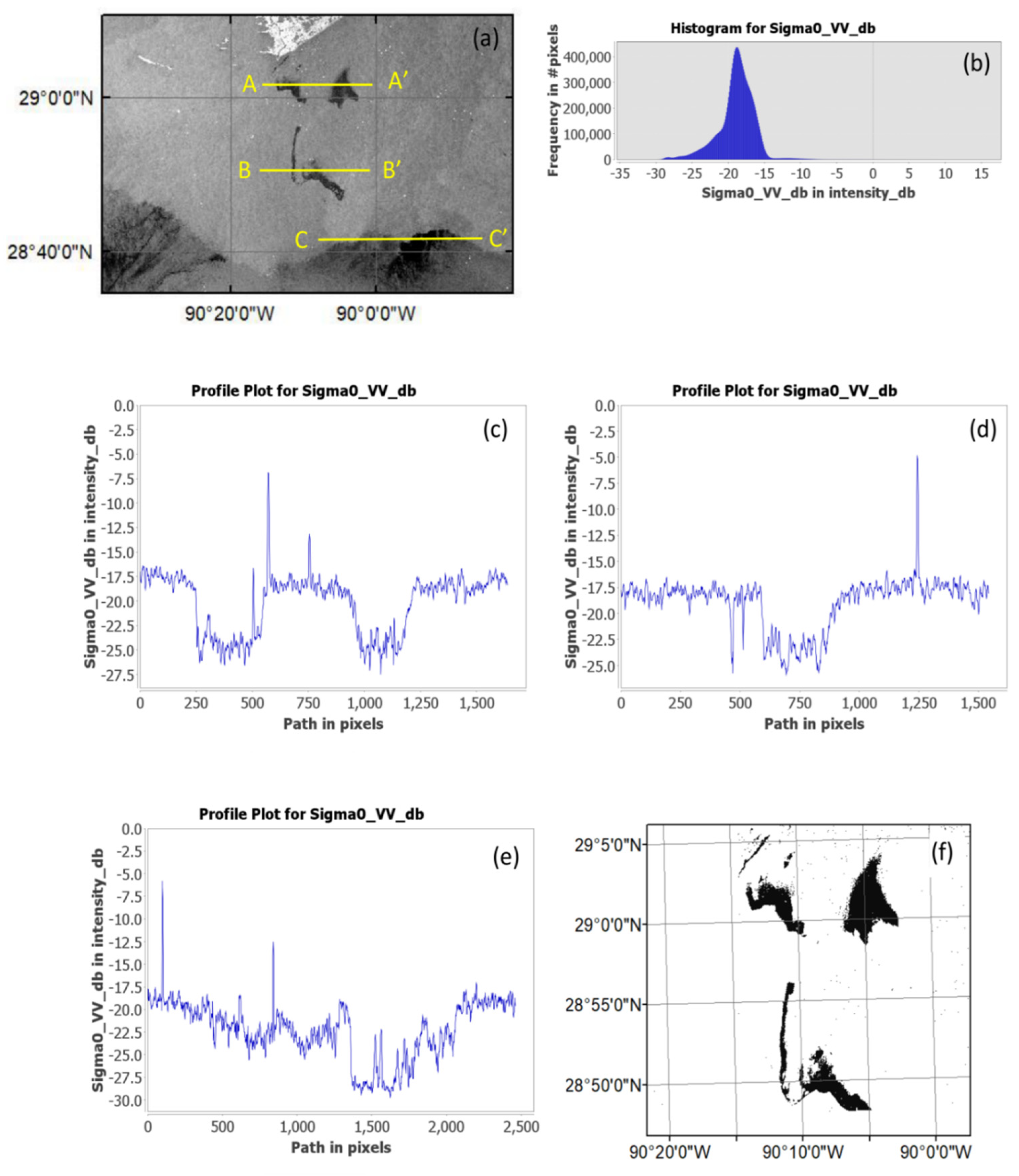
3.1. Sentinel-1A SRS Data

Figure 3a shows the oil spill in the Gulf of Mexico acquired from the Sentinel-1A preprocessed image data on 10 September 2021. In order to highlight the oil spill area, the ML supervised classification was applied to the Sentinel-1A preprocessed image data, choosing two classes: oil and seawater (Figure 3f). ML estimation is obtained from European Space Agency (ESA) SNAP toolbox software.
The black area shows the potential affected areas for oil spills in seawater areas. The “look-alike” effect is the disadvantage of SAR satellites’ oil spill detection methods, including the Sentinel-1A image [30]. In order to distinguish the typically calm sea slick from oil spill patches, it should be supported with sensors such as Landsat-8 and Sentinel-2 to strengthen the SAR processing findings. In addition, the histogram information with the different cross-sections in the image that correspond to the black spots can be analyzed to define the oil and non-oil spill areas. Figure 3b depicts the Sigma0 VV polarization histogram of Sentinel-1 image in db ranges from −5 to −30 db. Figure 3c–e show AA’, BB’, and CC’ cross-sections of Sentinel-1 images in yellow, respectively.
In these cross-sections, the seawater is about −17.5 db. The cross-section penetrating the oil spill area shows values between −22.5 db and −25 db (AA’ and BB’, respectively). The values corresponding to the black spot are about −27.5 db after analyzing the CC’ cross-section. In this cross-section, values of about −25 db may cause misinterpretation of the oil spill area as this area does not coincide with the optical images PCA. In the following sections, suppose the possible oil spill area accumulated around AA’ and BB’ cross-sections when compared with the PCA images represented. Calm Sea slick can be regarded as the region that includes the CC’ cross-section. The ML classification results are shown in Figure 3f to show oil and non-oil spill areas by applying area of interest polygons by the user for oil and non-oil spill regions to the algorithm. The affected region for the oil spill with the black spots almost coincides with the region from the optical images PCA.

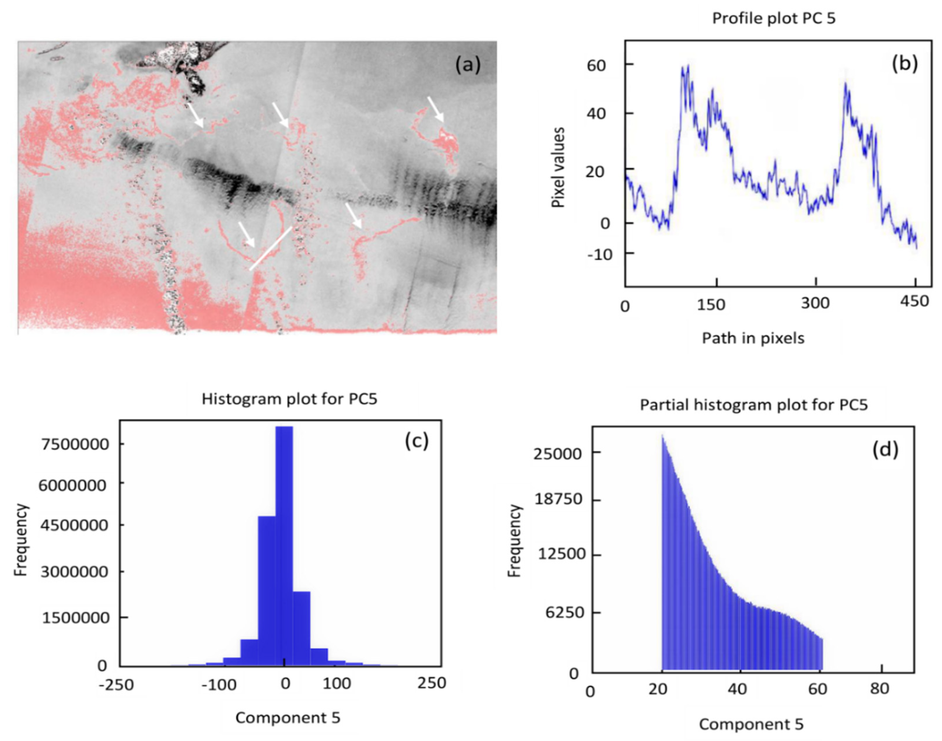
3.2. Landsat-8 SRS Data

For the next step, PCA is applied to the Sentinel-2 and Landsat-8 satellite image bands to support the findings from the Sentinel-1 data. The information from all bands is stacked into the PCA components by reducing noise in the SRS images. This is an advantage for analyzing the oil spill images. Table 2 and Table 3, shows input and output for the Sentinel-2 and Landsat-8 are 12 and 8 bands respectively. After the PCA components are estimated, it is analyzed for oil spills by defining different threshold values. In order to define the threshold values, the PCA cross-section, histogram, and partial histogram are examined.
PCA component 4 (Figure 4a), the cross-section profile plot of component 4 (Figure 4b), the component 4 histogram (Figure 4c), and the component 4 partial histogram for predefined values (Figure 4d) are given for Landsat-8 band on 3 September 2021. The cross-sections are used to define the threshold values to distinguish the oil spill from the sea. The outcome shows good separation selected as PCA component 4. The cross-section profile plot values change between −50 and 250 (Figure 4b).
The values around −50 to 0 show the seawater. The threshold values between 150 and 200 are defined for oil spill detection. The oil spill is shown in red as it overlaps the principal component 4 and is shown in Figure 4a. These threshold values partially determine the area with an oil spill. The misclassification is also an outlier outside of the pixel oil spill area. This can be related to the pixel outside similarity to the oil spill pixels. The PCA histogram was also provided for the analysis in Figure 4c. The image pixels distribution is also standard.

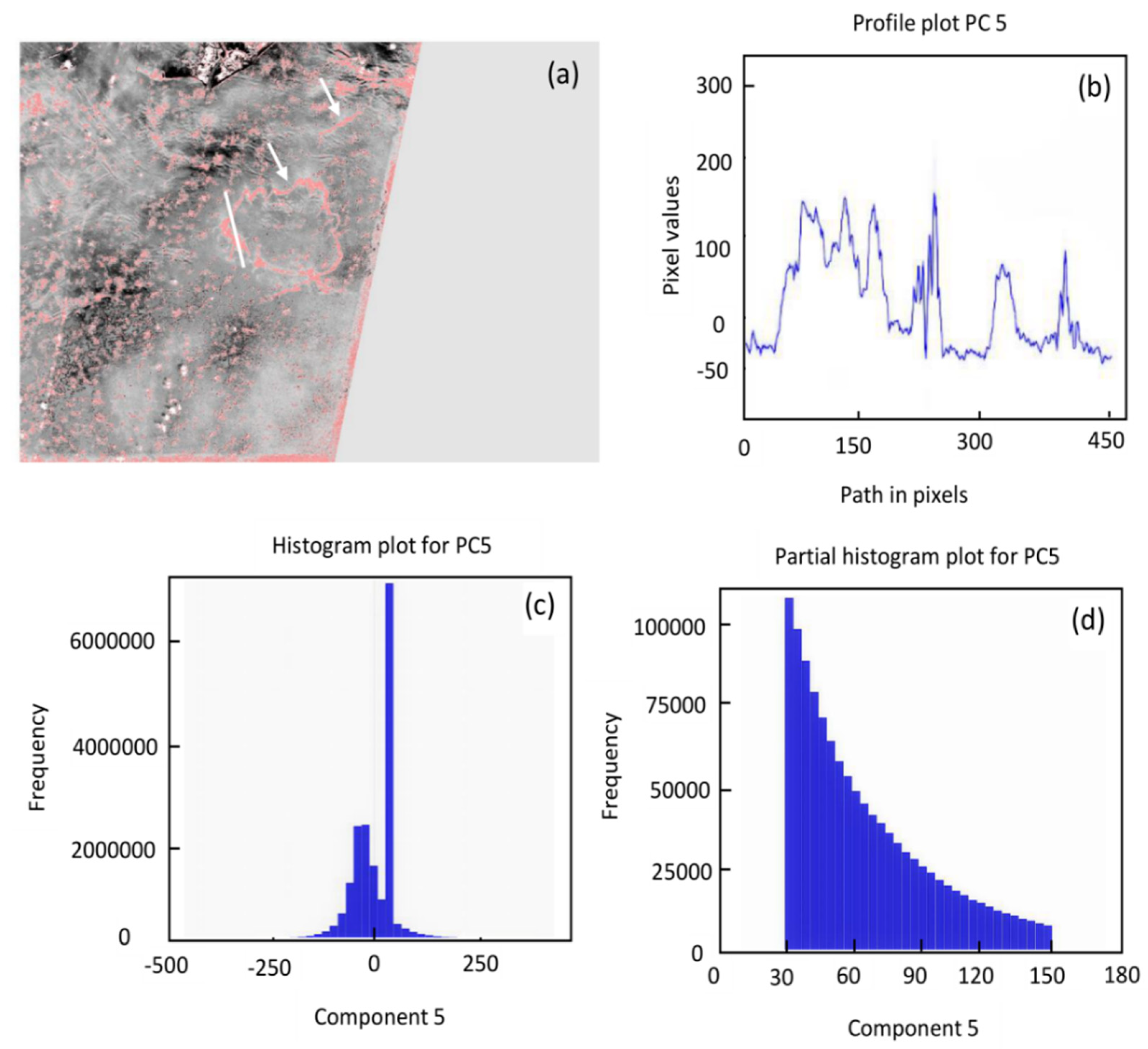
3.3. Sentinel-2 SRS Data

Figure 5a shows the PCA component 2 from Sentinel-2 bands on 2 September 2021. Figure 5b shows cross-section profile plot of component 2 (white line). Figure 5c depicts the component 2 histogram. Figure 5d is the component 2 partial histogram for predefined values. The cross-sections are used to define the threshold values used to distinguish the oil spill from the seawater. The cross-section is applied to all PCA components in the first stage. From these, the cross = section that shows good separation was selected as PCA component 2. The cross-section profile plot values change between 0 and −1500 (Figure 5b). The values around zero shows the seawater. The threshold values between −1500 and −750 are defined for oil spill detection. The oil spill is shown in red as it is overlapped onto principal component 2; this is shown in Figure 5a.
The area with an oil spill is primarily determined using these threshold values; it is shown with a white arrow. There are also some outliers outside the oil spill area, as pixels are misclassified. This can be related to the pixel values outside the spill that are similar values to the oil spill pixel areas value. The PCA histogram was also provided for the analysis in Figure 5c. This figure, a high value of around 500, shows an empty area. The partial histogram shows that the oil spill region is at the standard distribution curve edge. The partial histogram shows that the oil spill region is in the middle of the standard distribution curve. However, PCA Figure 5 shows a different grey level, making it harder to distinguish oil spills from the seawater.
Figure 6a shows the PCA component 5 from Sentinel-2 bands on 4 September 2021. Figure 6b shows cross-section profile plot of component 5. Figure 6c depicts the component 5 histogram. Figure 6d is the partial histogram of component 5 for predefined intervals. On this day, the component that shows good separation from these cross-sections was selected as PCA component 5. The cross-section profile plot values change between −10 and 60 (Figure 6b); the values around 10 show the seawater.
The threshold values between 20 and 60 are defined for oil spill detection. The oil spill is shown in red as it overlaps the principal component 5; this is shown in Figure 6a. These threshold values primarily determine the area with an oil spill. The PCA histogram was also provided for the analysis in Figure 6c. The values range between −300 to 300. The image pixels distribution is also standard. The partial histogram shows the oil spill region in the standard distribution middle curve.
Figure 7a shows the PCA component 5 Figure 7b shows the cross-section profile plot of component 5. Figure 7c shows the component 5 histogram. Figure 7d shows the component 5 partial histogram from Sentinel-2 bands on 7 September 2021. On this day, PCA component 5 shows good contrast for separating oil from the sea. The cross-section profile plot values change between −50 and 200 (Figure 7b). The values around −30 show the sea. The threshold values between 30 and 150 are defined for oil spill detection. The oil spill is shown in red on the principal component 5 images in Figure 7a. These threshold values primarily determine the area with an oil spill. However, there are also high outliers at the cloud border. This can be related to pixel similarity outside the oil spill pixels. The PCA histogram provided for the analysis is in Figure 7c.
The values range from −400 to 400. The image pixels distribution is also normal, except with the high corresponding to the empty region in the image. The partial histogram shows that the oil spill region is between the middle and the standard distribution curve right-hand side. The analysis in Figure 4, Figure 5, Figure 6 and Figure 7 represent the PCA component’s output to demonstrate the oil spill region spectral separability from the other objects using the threshold technique.
PCA is a transformation method used to obtain maximum variance directions using eigenvector and eigenvalues. The multispectral transformation data with PCA results in different principal components include the information related to different degrees with the original image details, such as oil, water, and land.

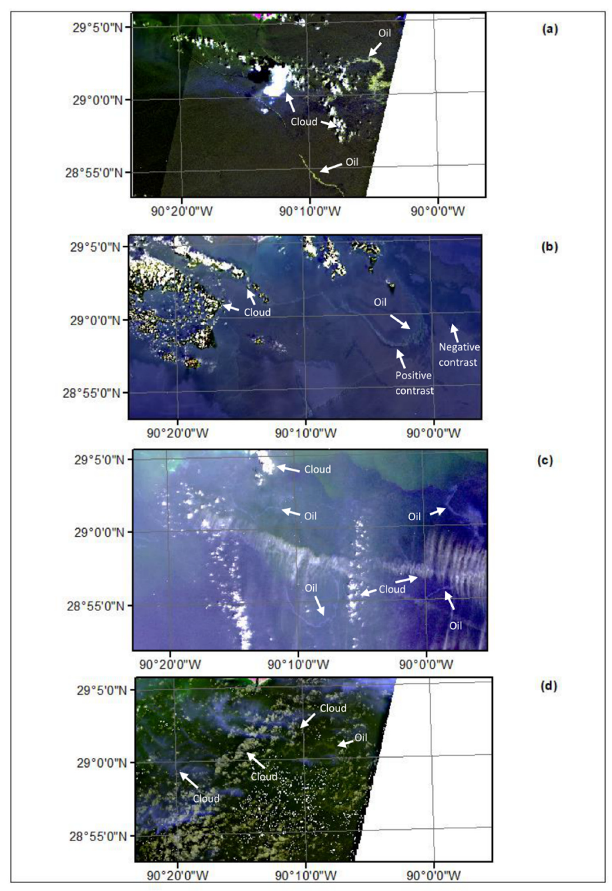
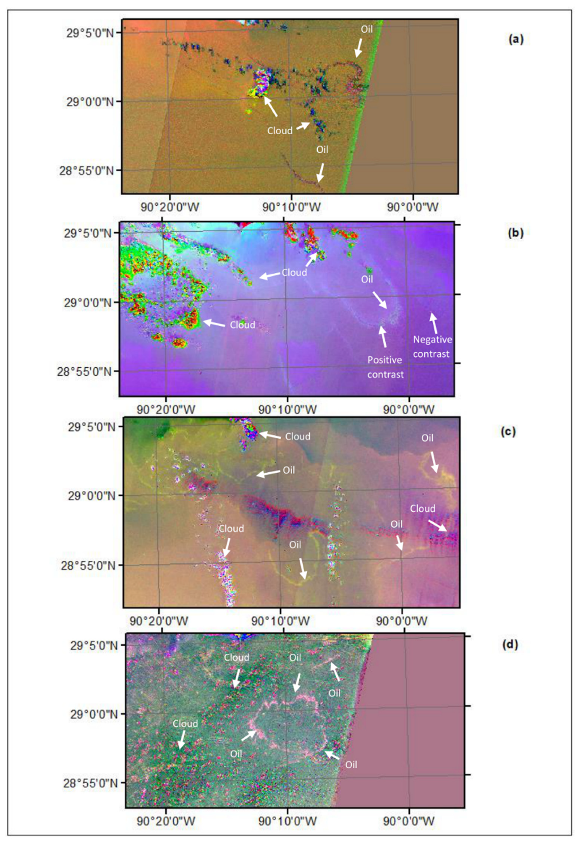
3.4. Natural Color Composite and RGB Image of PCA Bands

Natural color composite images from Sentinel 2 and Landsat 8 satellites using band 4, band 3, and band 2 (Figure 8) are constructed. In order to obtain a visible image, these band combinations should be filtered (preprocessing), applying gamma stretch and clipping extreme pixels from images.
Figure 8a is a natural color composite obtained from Sentinel-2 satellite bands on 2 September 2021. The oil spill can easily be seen as olive-colored on the Sea Surface Water (SSW). The clouds are white, and the clouds edge is olive in color, as with an oil spill.
Figure 8b is a natural color composite acquired from Landsat-8 satellite bands on 3 September 2021. The image shows the oil spill region with bright and dark pixels on the SSW. These pixels can be noted as oil spills.
The oil spill contrast can change if the dampening effect modifies the reflected sun light behavior as a specular reflection. The sun glint occurs as a result of the sunlight’s specular reflection on the calm SSW. The sun glint pattern depends on features such as viewing geometry concerning the sun, the sensor type and height on the platform, the SSW roughness, and atmospheric conditions such as cloud cover and aerosol. SSW roughness depends on the wind, internal waves, currents, eddies, ship wakes, oil slicks, and atmospheric conditions. Positive contrast was obtained when the conditions for the specular reflection from a smooth surface took place, resulting in sun glint (bright pixels). Conversely, the SSW can be seen as dark in the image from the other viewing angle as a non-specular reflection.
In our study, these behaviors can be seen in Figure 8b, with positive (bright) and negative (dark) contrast in the image corresponding to the oil spill region. The positive contrast region is mentioned as a thicker oil spill from the National Oceanic and Atmospheric Administration (NOAA) National Environmental Satellite, Data, and Information Service (NESDIS) marine pollution surveillance report, whereas negative contrast can be noted as a possible (but unconfirmed) oil spill. This report supports our study findings. The remaining images in Figure 8 do not show a negative contrast that can be seen visually. The effects that manage the sun glint make occurrence interpretation very difficult whenever determining an oil spill, especially in a larger area for negative contrast.
In Figure 8c, Sentinel-2 bands are provided from 4 September 2021. In this image, the clouds are white and grey and the seawater is dark blue. The oil spill is in light purple. Figure 8d is a natural color composite obtained from Sentinel-2 satellite bands on 7 September 2021. There are two types of clouds (blue and grey). The SSW is dark green. The oil spill area can barely be seen, in yellow, because the image has a complex structure and requires an enhancement technique to distinguish the region with the oil spill from those around it. The primary restrictive factor for oil spill determination using the original RGB image are clouds and the sea surface behavior regarding the sun glint effect, resulting in negative contrast for the study scope. The image processing techniques can be efficiently used to remove the cloud’s adverse effect and highlight the oil spill area. In Figure 8a, the oil spill area is distinct from clouds and can be easily separated from SSW. A similar situation can be said for Figure 8b as well. However, Figure 8c,d must be processed for oil spills as the clouds degrade the image quality.
This study suggests applying PCA as an image enhancement technique as a result of these drawbacks. In PCA, satellite sensors’ image bands that include similar information are decorrelated to enhance the images. After the transformation, most information is included in the principal components’ first parts. The principal component’s output in the grey image has different contrast levels with the reduced noise. From these components, the maximum variance direction does not mean that it shows the oil spill area with good spectral separation from other objects. So, visual inspection needs to be carried out to obtain a good separation between the principal components. As each principal component in different directions has a different variance, they are visually analyzed in the principal component images for the oil spill area. For example, in the Sentinel-2 image from 2 September 2021, oil shows good separation in the PCA component 2; for the Landsat-8 image from 3 September 2021, the PCA component 4 depicts good contrast.
As the principal component’s analysis aims to highlight oil spill areas, a problem arises with the similarity of pixel values of oil and other features after the original image conversion with PCA. The grey image contrast level for pixel values can be dark in some parts and bright in others. The contrast changes in the principal component image produce gradients that can be used to separate oil from seawater, clouds, and land. Threshold values mathematically used to produce distinct oil spill regions cannot be carried out precisely. Because the pixel values spectral reflectance from the SRS sensor managed by the cloud coverage, fog, oil, marine optical properties, and film thickness, some parts of the effected image coincide with the oil spill spectral response even after PCA transformation.
The threshold for a selected interval principal component can be used during the first stage to separate the image oil spill area. The general drawback of using threshold values is the misclassification of pixels due to the similar pixel values for oil and other features. This situation can confuse the process of distinguishing oil from other features. Cloud and contrast changes in the sea can be related to decision-making confusion. It is not easy to interpret the results. The PCA RGB color composite can be used to reduce the misinterpretation of the results of the principal components. These unclassified pixels can be addressed or eliminated using the selected principal component color composite. The oil spill region can be visualized more easily using this technique.
The RGB color composite image from the PCA output bands for Sentinel-2 (12 bands) and Landsat-8 (8 bands) is constructed using three principal components that represent the oil spills’ high visibility (Figure 9) for the different days. For example, the Sentinel-2 main components output band (6, 5, and 4) are provided in Figure 9a on 2 September 2021 using the RGB image. In this figure, the purple, red, and black region is the oil spill area, and the clouds are dark blue and a mixture of purple, yellow, and green. The remaining area is the SSW. The clouds and oil spill area show a similar texture and are accumulated in a particular region. The clouds can be discriminated as a volumetric shape in the figure. This signature is shown with a white arrow. After the PCA, the oil spill area is easily separated from clouds and seawater.
The RGB image from the principal component output (6, 4, and 3) band are shown in Figure 9b from Landsat 8 on 3 September 2021. This figure’s light purple and white region is an arc of oil spill areas. This region can be regarded as the positive contrast area when compared with natural color composite (Figure 8b). There are also some regions with purple and light purple that can be noted as negative contrast, shown with the arrow in Figure 9b. These negative and positive contrasts, related to sun glint, make interpretation difficult as it depends on parameters mentioned earlier. All this information is required to properly detect oil spills. The clouds are green and red. The remaining purple area is the SSW.
The other RGB image is constructed using the Sentinel-2 principal components output band (6, 5 and 4) from 4 September 2021 (Figure 9c). In this figure, the yellow region is the oil spill area. The clouds are purple and white. The remaining area is sea water. In this figure, the color separation is distinctive and unmistakable. The last RGB image from the principal components output band (5, 8 and 12) can be given in Figure 9d from 7 September 2021. In this figure, the pink region is the oil spill area. Clouds primarily dominate the remaining area and are seen as green and magenta. PCA (Figure 9d) successfully distinguishes oil spills from an image highly dominated by clouds when compared with the natural composite image (Figure 8d).
It can be seen in Figure 9 that the oil spill area shown using the different band combinations has different colors. This situation can be explained by the principal components from each image having unique values and losing their reflectance values after PCA transformation. The band combination is realized with visual inspection components highlighting the oil spill area. The negative contrast effect can loosely be seen after the PCA transformation in Figure 9b. This is because the original bands’ RGB image is complex, and it is not easy to interpret the results for PCA (Figure 9b) without the exact location ground truth knowledge data. However, the positive contrast can be interpreted as an oil spill area. The oil spill direction was analyzed after determining the oil spill area using PCA.
Figure 10 demonstrates the oil spill spread direction for the selected time intervals. The selected satellite image period for the analysis is one week earlier and two weeks after the event in the Gulf of Mexico around Port Fourchon. The significant oil discharge behavior in the Gulf of Mexico can be noted as natural oil seepages and oil spills from platforms and pipelines. In order to focus on the oil spill from platforms and pipelines, these two phenomena must be addressed as our study is concerned with these effects.
A studied by Najoui et al. [52] discussed the natural oil seepages in the Gulf of Mexico. They stated that natural oil seepages with a curved geometric shape are managed by the wind and currents. This pattern is focused on the same place and at an almost fixed point in time; this is regarded as an oil discharge type specific property.
Oil spills from platforms or pipelines have an irregular geometric shape that affects larger areas. This oil spill pattern is repeatedly seen on different images acquired on different days. The other property of an oil spill is the nearness to oil platforms and pipelines. MacDonald et al. [53] demonstrated that the natural oil spill was primarily positioned offshore, far from the coastline in the Gulf of Mexico. They also found the natural oil seepage to continuous, repeated, and to have a curvilinear pattern in a fixed point. Concerning the stated explanation, the pipelines position and platforms are inserted in Figure 1 and Figure 10 alongside the oil spill areas to show the spread of an oil spill caused by Hurricane Ida [54].
The oil platforms and pipelines are located near the oil spill area. The oil spread moves from one image to another and has an irregular geometric shape. This can be related to the oil discharge from oil platforms and pipelines, as explained in the studies mentioned above. The oil spill area does not emanate from one point in the visual data inspection. It is moving without a connection to a fixed position.

3.5. ML Classification

In order to strengthen results, all the information is combined to demonstrate the oil spills progress using ML classification. Figure 8a shows a clear distinction between oil and water after data image preprocessing. The remaining figures show different mixed features on the SSW, including clouds, that can make hard to interpret the images even after preprocessing the image using different parameters. As such, a more efficient tool was used as PCA. The features provide much more contrast, making it easier to distinguish polygons for ML classification after the PCA. This classification is used to show the daily progress of the oil spill region.
There are a variety of classification techniques that have advantages and disadvantages concerning the selected parameters for training. Li et al. [55] studied the performance of 13 supervised and two unsupervised classification algorithms. They found that the proposed methods’ accuracies are greater than 80%, with the highest (89%) for ML classification. The advantage of ML classification advantage is that it needs fewer pixels than other methods to reach high accuracy values. On the other hand, the proposed supervised methods have similar and high accuracies if the training parameters are selected carefully and adequately. This study proposes ML classification two to determine oil and non-oil spill areas.
As shown in Figure 10, the oil spill areas offer a sharper pattern and the edges or gradients are visible. The noise in the image was reduced as the components were uncorrelated. The ML classification has been applied to the SRS data PCA component results to monitor the oil spills after the event. In this case, only oil spills can be named the studied class and, due to this interest, this study only focuses on obtaining an oil class to overlap images from different days. First, three classes are defined (cloud, land and sea) other than the oil spill. Then, the classified image is reduced to one class represented as a non-oil spill region using reclassifying from the obtained three classes. Next, the classification is defined for SAR data: oil spill and non-oil spill. Finally, the ground truth data is defined from Google Earth and visual inspection of the oil spill area. The classification is carried out for all days and sensors. For accuracy assessment, 100 randomly selected samples from the classified image were analyzed and compared with the ground truth data and visual inspection.
The overall accuracy metric is used that can be estimated by dividing the correctly determined pixels for classes by the reference pixels total number. The overall accuracy is 86% (Sentinel-2, 2 September 2021), 89% (Landsat-8, 3 September 2021), 85% (Sentinel-2, 4 September 2021), 80% (Sentinel-2, 7 September 2021) and 88% (Sentinel-1 SAR, 10 September 2021). The classification accuracy is good enough to show the progress of the oil spill. In the classification, the spectral response of oil and clouds in the SRS bands data are similar, resulting in some unwanted pixels at the cloud border. This situation makes classification more complex in the classification stage as it is difficult to distinguish oil from clouds. Therefore, it requires more attention during the processing.
Figure 10 is constructed by overlapping all the one-class images from the days used. In this figure, the oil spill spread from Sentinel-2 bands is shown in turquoise on 2 September 2021 (Figure 10), red on 4 September 2021 (Figure 10), and dark blue on 7 September 2021 (Figure 10). The oil spill spread from Landsat 8 was green on 3 September 2021 (Figure 10). The oil spill area from the Sentinel-1 images is shown in black on 10 September 2021 (Figure 10). The Gulf Stream information near the studied area is added to Figure 10 as a red arrow to the oil spill direction predicted. The Gulf Stream current in the Gulf of Mexico is maintained by the Eddies and the main gulf loop current [56].The main Gulf Stream current is far from the studied area (about 60 km south). The movement directions relate to the purple line and circle.
The circle is positioned at the oil spill center for the related day. In the upper part of Figure 10, the oil spill movement direction can be seen moving from west to east by following the purple line and circle. This line is parallel to the Gulf current direction. The region in turquoise (2 September 2021) moves to east on the next day, shown by green and followed by red. This area is correlated with the part obtained from the SAR sensor. This correlation can be noted as the oil spill detected from radar data is distinct, as a result of the “look-alike” effect. The second spread direction shows another polluted region as a result of the oil spill. The area from turquoise, green, and red moves slowly when compared with the first spread direction seen by following the purple line and circle. This movement increased over the last day, as shown in dark blue. The oil spill event can be identified from optical and radar sensor images and correlated.

3.6. Landsat 8 Thermal Band Analysis

In the last step, the thermal band response to the oil spill area is studied using original and filtered images to show the thermal data usability in oil spill studies. The Landsat-8 satellite thermal band is converted to the LST using Equation (1) and parameters from Table 2 for oil spill analysis.
Figure 11a shows the estimated LST values from thermal band 10 for Landsat 8 on 03.09.2021. The values range between 301.37 K and 304.57 K for the selected region, with 12 time intervals with a color bar in brown. The thermal band may respond to the oil spill [30]. This response can be seen in the figure in white and brown, with values between 301 and 302 K. Different filters are applied to the LST image to highlight the oil spill area in the thermal band. Three filters applied to the LST image can separate the oil spill area from the sea, represented in Figure 11b–d. The LST Mean filter with 3 × 3 Kernel is given in Figure 11b. The oil spill area is black and shown by the red arrow.
The LST High-pass filter with 3 × 3 Kernel is represented in Figure 11c. The oil spill region in dark black can be distinguished from the sea. The High-Pass filter result is provided in Figure 11d as the kernel degree is increased to 5 × 5. The oil spill area is in white. The arc-type signature can easily be seen in Figure 11.
Two cross-sections with the yellow line are taken from Figure 11a with AA’ and BB’ to show the changes in LST as a result of the oil spill. The cross-section plots are given in Figure 12a,b. The cross-section profile plot of LST takes values between 302.8 K and 304 K in Figure 12a. The LST values drop from 304 K to 302.8 K, represented by a red circle in the oil spill area. LST decreases from 304 to 303.8 K in the second region cross-section profile plot.
The second cross-section profile plot is provided in Figure 12b to validate the results from Figure 12a. Similar results can be found in this figure, with values ranging from 302.6 K to 304 K. The LST values decreased from 304 K to 302.6 K, represented by a red circle in the oil spill area. LST decreases from 303.8 to 303.5 K in the second region.

4. Conclusions

Some researchers determine an oil spill using SAR, while others use optical images in oil spill detection. The cloud coverage, satellite revisit time, spatial resolution, and oil spill thickness restrict the definition of the affected region. Looking at the problem using only one method is not reliable. As each method has advantages and disadvantages, it is essential to obtain the correct balance between them for optimized results because of the challenging subject properties. The complexity of the mathematical concepts does not mean a method is the best for oil spill detection, as each oil spill problem has a different structure.
The PCA method is a dimension reduction technique for highlighting suppressed features in an image that can be quickly applied to all kinds of data. The oil spill region could not be determined in some images directly; it requires methods, such as PCA, to acquire this information. However, some images with 80% cloud coverage (Sentinel-2, 7 September 2021) can be handled by PCA bands color composites for oil spill determination in the region (Sentinel-2, 4 September 2021). The other finding is that the images’ gradients are more transparent for oil spills as the redundant information is reduced because the PCA uncorrelated components after conversion.
Because of these drawbacks, this study suggests applying PCA as an image enhancement technique. In PCA, satellite sensors’ image bands that include similar information are decorrelated to enhance the images. After the transformation, most information is included in the principal components’ first parts. The principal components output in the grey image has different contrast levels with reduced noise. From these components, the maximum variance direction does not mean that it shows the oil spill area with good spectral separation from other objects. As such, a visual inspection must be conducted to obtain a good separation between the principal components. They are visually analyzed in the principal component images for the oil spill area, as each principal component in different directions has a different variance.

Author Contributions

Conceptualization, N.A.; methodology, N.A. and M.M.N.; software, N.A. and M.M.N.; validation, N.A., M.M.N., A.H., D.A.G. and G.S.; formal analysis, N.A., M.M.N., A.H., D.A.G. and G.S.; investigation, N.A., M.M.N., A.H., D.A.G. and G.S.; resources, N.A., M.M.N., A.H., D.A.G. and G.S.; data curation, N.A., M.M.N., A.H., D.A.G. and G.S.; writing—original draft preparation, N.A., M.M.N., A.H., D.A.G. and G.S.; writing—review and editing, N.A., M.M.N., A.H., D.A.G. and G.S.; visualization, N.A., M.M.N. and A.H.; supervision, D.A.G. and G.S.; project administration, D.A.G. and G.S. All authors have read and agreed to the published version of the manuscript.

Funding

This research was funded by the European Union’s Horizon 2020 European Green Deal Research and Innovation Program (H2020-LC-GD2020-4), grant number No. 101037643–ILIAD (Integrated Digital Framework for Comprehensive Maritime Data and Information Services). The article reflects only the authors’ view and that the Commission is not responsible for any use that may be made of the information it contains.

Data Availability Statement

Not applicable.

Acknowledgments

The author would like to thank the European Space Agency (ESA) for providing Sentinel-1, Sentinel-2 satellites data (Supported by Copernicus open-access platform) and the United States Geological Survey (USGS) for Landsat-8 satellite data. Finally, the satellite imagery was processed using SNAP software (open-access).

Conflicts of Interest

The authors declare no conflict of interest.

References

  1. Marignani, M.; Bruschi, D.; Garcia, D.A.; Frondoni, R.; Carli, E.; Pinna, M.S.; Cumo, F.; Gugliermetti, F.; Saatkamp, A.; Doxa, A.; et al. Identification and prioritization of areas with high environmental risk in Mediterranean coastal areas: A flexible approach. Sci. Total Environ. 2017, 590–591, 566–578. [Google Scholar] [CrossRef] [PubMed]
  2. Vargas, G.C.; Au, W.W.; Izzotti, A. Public health issues from crude-oil production in the Ecuadorian Amazon territories. Sci. Total Environ. 2020, 719, 134647. [Google Scholar] [CrossRef] [PubMed]
  3. Di Girolamo, P.; Piras, G.; Pini, F. The effect of COVID-19 on the distribution of PM10 pollution classes of vehicles: Comparison between 2020 and 2018. Sci. Total Environ. 2022, 811, 152036. [Google Scholar] [CrossRef]
  4. Nunziata, F.; Gambardella, A.; Migliaccio, M. A unitary Mueller-based view of polarimetric SAR oil slick observation. Int. J. Remote Sens. 2012, 33, 6403–6425. [Google Scholar] [CrossRef]
  5. Caruso, M.J.; Migliaccio, M.; Hargrove, J.T.; Garcia-Pineda, O.; Graber, H.C. Oil spills and slicks imaged by synthetic aperture radar. Oceanography 2013, 26, 112–123. [Google Scholar] [CrossRef] [Green Version]
  6. Zhai, J.; Mu, C.; Hou, Y.; Wang, J.; Wang, Y.; Chi, H. A Dual Attention Encoding Network Using Gradient Profile Loss for Oil Spill Detection Based on SAR Images. Entropy 2022, 24, 1453. [Google Scholar] [CrossRef]
  7. Sun, Z.; Sun, S.; Zhao, J.; Ai, B.; Yang, Q. Detection of Massive Oil Spills in Sun Glint Optical Imagery through Super-Pixel Segmentation. J. Mar. Sci. Eng. 2022, 10, 1630. [Google Scholar] [CrossRef]
  8. Magalhães, K.M.; de Souza Barros, K.V.; de Lima, M.C.; de Almeida Rocha-Barreira, C.; Rosa Filho, J.S.; de Oliveira Soares, M. Oil spill + COVID-19: A disastrous year for Brazilian seagrass conservation. Sci. Total Environ. 2021, 764, 142872. [Google Scholar] [CrossRef]
  9. Yaghmour, F.; Els, J.; Maio, E.; Whittington-Jones, B.; Samara, F.; El Sayed, Y.; Ploeg, R.; Alzaabi, A.; Philip, S.; Budd, J.; et al. Oil spill causes mass mortality of sea snakes in the Gulf of Oman. Sci. Total Environ. 2022, 825, 154072. [Google Scholar] [CrossRef] [PubMed]
  10. Nunes, B.Z.; Zanardi-Lamardo, E.; Choueri, R.B.; Castro, Í.B. Marine protected areas in Latin America and Caribbean threatened by polycyclic aromatic hydrocarbons. Environ. Pollut. 2021, 269, 116194. [Google Scholar] [CrossRef]
  11. Available online: https://www.itopf.org/knowledge-resources/data-statistics/statistics/ (accessed on 21 February 2023).
  12. Sun, S.; Lu, Y.; Liu, Y.; Wang, M.; Hu, C. Tracking an Oil Tanker Collision and Spilled Oils in the East China Sea Using Multisensor Day and Night Satellite Imagery. Geophys. Res. Lett. 2018, 45, 3212–3220. [Google Scholar] [CrossRef]
  13. Deis, D.R.; Mendelssohn, I.A.; Fleeger, J.W.; Bourgoin, S.M.; Lin, Q. Legacy effects of Hurricane Katrina influenced marsh shoreline erosion following the Deepwater Horizon oil spill. Sci. Total Environ. 2019, 672, 456–467. [Google Scholar] [CrossRef]
  14. Fingas, M.; Brown, C.E. Oil Spill Remote Sensing: A Review. In Oil Spill Science and Technology: Prevention, Response, and Clean Up; Fingas, M., Ed.; Elsevier: Burlington, MA, USA, 2011; pp. 111–169. Available online: http://store.elsevier.com/product.jsp?isbn=9781856179430 (accessed on 21 February 2023).
  15. Laneve, G.; Luciani, R. Developing a satellite optical sensor based automatic system for detecting and monitoring oil spills. In Proceedings of the 2015 IEEE 15th International Conference on Environment and Electrical Engineering (EEEIC), Rome, Italy, 10–13 June 2015; pp. 1653–1658. [Google Scholar] [CrossRef]
  16. Balogun, A.L.; Yekeen, S.T.; Pradhan, B.; Althuwaynee, O.F. Spatio-temporal analysis of oil spill impact and recovery pattern of coastal vegetation and wetland using multispectral satellite Landsat 8-OLI imagery and machine learning models. Remote Sens. 2020, 12, 1225. [Google Scholar] [CrossRef] [Green Version]
  17. Santilli, G.; Marzialetti, P.; Laneve, G. A novel sinergy between remote sensing and GIS for oil spill detection on satellite imagery. In Proceedings of the 34th International Symposium on Remote Sensing of Environment, the GEOSS Era: Towards Operational Environmental Monitoring, Sydney, Australia, 10–15 April 2011; Available online: https://www.isprs.org/proceedings/2011/ISRSE-34/211104015Final00093.pdf (accessed on 21 February 2023).
  18. Dasari, K.; Anjaneyulu, L.; Nadimikeri, J. Application of C-band sentinel-1A SAR data as proxies for detecting oil spills of Chennai, East Coast of India. Mar. Pollut. Bull. 2021, 174, 113182. [Google Scholar] [CrossRef] [PubMed]
  19. Gambardella, A.; Giacinto, G.; Migliaccio, M.; Montali, A. One-class classification for oil spill detection. Pattern Anal. Appl. 2010, 13, 349–366. [Google Scholar] [CrossRef]
  20. Olita, A.; Cucco, A.; Simeone, S.; Ribotti, A.; Fazioli, L.; Sorgente, B.; Sorgente, R. Oil spill hazard and risk assessment for the shorelines of a Mediterranean coastal archipelago. Ocean Coast. Manag. 2012, 57, 44–52. [Google Scholar] [CrossRef]
  21. Alves, T.M.; Kokinou, E.; Zodiatis, G.; Lardner, R.; Panagiotakis, C.; Radhakrishnan, H. Modelling of oil spills in confined maritime basins: The case for early response in the Eastern Mediterranean Sea. Environ. Pollut. 2015, 206, 390–399. [Google Scholar] [CrossRef] [Green Version]
  22. Ferraro, G.; Bernardini, A.; David, M.; Meyer-Roux, S.; Muellenhoff, O.; Perkovic, M.; Tarchi, D.; Topouzelis, K. Towards an operational use of space imagery for oil pollution monitoring in the Mediterranean basin: A demonstration in the Adriatic Sea. Mar. Pollut. Bull. 2007, 54, 403–422. [Google Scholar] [CrossRef]
  23. Chrastansky, A.; Callies, U. Model-based long-term reconstruction of weather-driven variations in chronic oil pollution along the German North Sea coast. Mar. Pollut. Bull. 2009, 58, 967–975. [Google Scholar] [CrossRef] [Green Version]
  24. Krek, E.V.; Krek, A.V.; Kostianoy, A.G. Chronic oil pollution from vessels and its role in background pollution in the southeastern baltic sea. Remote Sens. 2021, 13, 4307. [Google Scholar] [CrossRef]
  25. Coppini, G.; De Dominicis, M.; Zodiatis, G.; Lardner, R.; Pinardi, N.; Santoleri, R.; Colella, S.; Bignami, F.; Hayes, D.R.; Soloviev, D.; et al. Hindcast of oil-spill pollution during the Lebanon crisis in the Eastern Mediterranean, July-August 2006. Mar. Pollut. Bull. 2011, 62, 140–153. [Google Scholar] [CrossRef]
  26. Alves, T.M.; Kokinou, E.; Zodiatis, G. A three-step model to assess shoreline and offshore susceptibility to oil spills: The South Aegean (Crete) as an analogue for confined marine basins. Mar. Pollut. Bull. 2014, 86, 443–457. [Google Scholar] [CrossRef]
  27. Chaturvedi, S.K.; Banerjee, S.; Lele, S. An assessment of oil spill detection using Sentinel 1 SAR-C images. J. Ocean Eng. Sci. 2020, 5, 116–135. [Google Scholar] [CrossRef]
  28. Rajendran, S.; Aboobacker, V.M.; Seegobin, V.O.; Al Khayat, J.A.; Rangel-Buitrago, N.; Al-Kuwari, H.A.; Sadooni, F.N.; Vethamony, P. History of a disaster: A baseline assessment of the Wakashio oil spill on the coast of Mauritius, Indian Ocean. Mar. Pollut. Bull. 2022, 175, 113330. [Google Scholar] [CrossRef]
  29. Marzialetti, P.; Laneve, G. Oil spill monitoring on water surfaces by radar L, C and X band SAR imagery: A comparison of relevant characteristics. In Proceedings of the 2016 IEEE International Geoscience and Remote Sensing Symposium (IGARSS), Beijing, China, 10–15 July 2016; pp. 7715–7717. [Google Scholar] [CrossRef]
  30. Arslan, N. Assessment of oil spills using Sentinel 1 C-band SAR and Landsat 8 multispectral sensors. Environ. Monit Assess. 2018, 190, 637. [Google Scholar] [CrossRef]
  31. Wang, L.F.; Xin, L.P.; Yu, B.; Ju, L.; Wei, L. A novel method for determination of the oil slick area based on visible and thermal infrared image fusion. Infrared Phys. Technol. 2021, 119, 103915. [Google Scholar] [CrossRef]
  32. El-Rahman, S.A.; Zolait, A.H.S. Hyperspectral image analysis for oil spill detection: A comparative study. Int. J. Comput. Sci. Math. 2018, 9, 103–121. [Google Scholar] [CrossRef]
  33. Liu, D.Q.; Luan, X.N.; Guo, J.J.; Cui, T.; An, J.B.; Zheng, R. A new approach of oil spill detection using time-resolved LIF combined with parallel factors analysis for laser remote sensing. Sensors 2016, 16, 1347. [Google Scholar] [CrossRef] [PubMed] [Green Version]
  34. Almulihi, A.; Alharithi, F.; Bourouis, S.; Alroobaea, R.; Pawar, Y.; Bouguila, N. Oil spill detection in sar images using online extended variational learning of dirichlet process mixtures of gamma distributions. Remote Sens. 2021, 13, 2991. [Google Scholar] [CrossRef]
  35. Ida1. 2022, p. 2022. Available online: https://www.space.com/hurricane-ida-oil-slicks-satellite-images (accessed on 10 February 2022).
  36. Ace, S. Ida2. 2022, pp. 2003–2005. Available online: https://www.washingtonpost.com/climate-environment/2021/09/07/oil-spill-hurricane-ida/ (accessed on 10 February 2022).
  37. Ida3. 2022, p. 6219248. Available online: https://www.voanews.com/a/usa_cleanup-boats-scene-large-gulf-oil-spill-followingida/6219248.html. (accessed on 10 February 2022).
  38. Ida4. 2022. Available online: https://news.sky.com/story/hurricane-ida-broken-pipeline-found-by-divers-in-search-for-gulf-of-mexico-oil-spill-12400534#:~:text=News%20%7C%20Sky%20News-,Hurricane%20Ida%3A%20Broken%20pipeline%20found%20by%20divers%20in%20search%20for,been (accessed on 21 February 2023).
  39. Mattthieu Bourbigot, Sentinel-1 Product Definition. 2012. Available online: https://sentinel.esa.int/documents/247904/1877131/Sentinel-1-Product-Definition (accessed on 21 February 2023).
  40. Suhet. Sentinel-1 User Handbook. European Space Agency. 2022. Available online: https://sentinel.esa.int/web/sentinel/user-guides/sentinel-1-sar (accessed on 21 February 2023).
  41. Ace, S. Esa. 2022, pp. 2003–2005. Available online: https://earth.esa.int/web/sentinel/technical-guides/sentinel-1-sar/products-algorithms/level-1-algorithms/ground-range-detected (accessed on 10 February 2022).
  42. Ulfa, E.H.; Sayler, K. Landsat 8 Collection 2 (C2) Level 2 Science Product (L2SP) Guide, USGS, EROS Sioux Falls, South Dakota, September 2020. SELL J. 2020, 5, 55. [Google Scholar]
  43. Bureau, E.; Richards, J.A. Supervised Classification Techniques. In Remote Sensing Digital Image Analysis; Springer: Berlin/Heidelberg, Germany, 2013; p. 30062. [Google Scholar] [CrossRef]
  44. Arslan, N. Identification of hotspots using different statistical methods in a region of manufacturing plants. Environ. Monit. Assess 2018, 190, 550. [Google Scholar] [CrossRef] [PubMed]
  45. Li, H.; Cui, J.; Zhang, X.; Han, Y.; Cao, L. Dimensionality Reduction and Clas-sification of Hyperspectral Remote Sensing Image Feature Extraction. Remote Sens. 2022, 14, 4579. [Google Scholar] [CrossRef]
  46. Ibarrola-Ulzurrun, E.; Marcello, J.; Gonzalo-Martin, C. Assessment of Com-ponent Selection Strategies in Hyperspectral Imagery. Entropy 2017, 19, 666. [Google Scholar] [CrossRef]
  47. Green, A.; Berman, M.; Switzer, P.; Craig, M. A transformation for ordering multispectral data in terms of image quality with implications for noise re-moval. IEEE Trans. Geosci. Remote Sens. 1988, 26, 65–74. [Google Scholar] [CrossRef] [Green Version]
  48. Hyvärinen, A.; Oja, E. Independent component analysis: Algorithms and applications. Neural Netw. 2000, 13, 411–430. [Google Scholar] [CrossRef] [PubMed] [Green Version]
  49. Chen, G.; Metz, M.R.; Rizzo, D.M.; Dillon, W.W.; Meentemeyer, R.K. Meentemeyer, Object-based assessment of burn severity in diseased forests us-ing high-spatial and high-spectral resolution MASTER airborne imagery. ISPRS J. Photogramm. Remote Sens. 2015, 102, 38–47. [Google Scholar] [CrossRef] [Green Version]
  50. Estornell, J.; Martí-Gavilá, J.M.; Sebastiá, M.T.; Mengual, J. Principal component analysis applied to remote sensing. Model. Sci. Educ. Learn. 2013, 6, 83–89. [Google Scholar] [CrossRef] [Green Version]
  51. Mather, P.M. Computer Processing of Remotely Sensed Images—An Introduction, 3rd ed.; Wiley: Chichester, UK, 2004; p. 2004. [Google Scholar]
  52. Najoui, Z.; Riazanoff, S.; Deffontaines, B.; Xavier, J.P. Estimated location of the seafloor sources of marine natural oil seeps from sea surface outbreaks: A new ‘source path procedure’ applied to the northern Gulf of Mexico. Mar. Pet. Geol. 2018, 91, 190–201. [Google Scholar] [CrossRef]
  53. MacDonald, I.R.; Garcia-Pineda, O.; Beet, A.; Daneshgar Asl, S.; Feng, L.; Graettinger, G.; French-McCay, D.; Holmes, J.; Hu, C.; Huffer, F.; et al. Natural and unnatural oil slicks in the Gulf of Mexico. J. Geophys. Res. Ocean. 2015, 120, 8364–8380. [Google Scholar] [CrossRef] [PubMed]
  54. BOEM, Bureau of Ocean Energy Management. 2022; p. 2022. Available online: https://www.data.boem.gov/Main/Mapping.aspx (accessed on 13 August 2022).
  55. Li, C.; Wang, J.; Wang, L.; Hu, L.; Gong, P. Comparison of Classification Algorithms and Training Sample Sizes in Urban Land Classification with Landsat Thematic Mapper Imagery. Remote Sens. 2014, 6, 964–983. [Google Scholar] [CrossRef] [Green Version]
  56. Zeng, X.; Li, Y.; He, R. Predictability of the Loop Current variation and eddy shedding process in the Gulf of Mexico using an artificial neural network approach. J. Atmos. Ocean. Technol. 2015, 32, 1098–1111. [Google Scholar] [CrossRef] [Green Version]
Figure 1. Study area of Port Fourchon oil spill event (The red squares show Gulf of Mexico).
Remotesensing 15 01460 g001
Figure 2. The workflow used in the study.
Remotesensing 15 01460 g002
Figure 3. (a) The data acquired from Sentinel-1A satellite for the oil spill on 10 September 2021, (b) Sentinel-1 image histogram, (c) AA’ cross-section profile plot of Sentinel-1 images, (d) BB’ cross-section profile plot of Sentinel-1 images, (e) CC’ cross-section profile plot of Sentinel-1 images, (f) Sentinel-1A for the oil spill ML classification results.
Remotesensing 15 01460 g003
Figure 4. (a) The PCA component 4 was estimated from Landsat 8 bands on 3 September 2021, (b) Cross-section profile plot of component 4, (c) Component 4 histogram, (d) Component 4 partial histogram for predefined values.
Remotesensing 15 01460 g004
Figure 5. (a) The PCA component 2 was estimated from Sentinel-2 bands on 2 September 2021, (b) Cross-section profile plot of component 2, (c) Component 2 histogram, (d) Component 2 partial histogram for predefined values.
Remotesensing 15 01460 g005
Figure 6. (a) The PCA component 5 estimated from Sentinel-2 bands on 4 September 2021, (b) Cross-section profile plot of component 5, (c) Component 5 histogram, (d) Component 5 partial histogram for predefined values.
Remotesensing 15 01460 g006
Figure 7. (a) The PCA component 5 estimated from Sentinel-2 bands on 7 September 2021, (b) Cross-section profile plot of component 5. 5, (c) Component 5 histogram, (d) Component 5 partial histogram for predefined values.
Remotesensing 15 01460 g007
Figure 8. Natural color composite. (a) Sentinel-2 (4, 3 and 2) bands on 2 September 2021, (b) Landsat-8 (4, 3 and 2) bands on 3 September 2021, (c) Sentinel-2 (4, 3 and 2) bands on 4 September 2021, (d) Sentinel-2 (4, 3 and 2) bands on 7 September 2021.
Remotesensing 15 01460 g008
Figure 9. PCA bands RGB image. (a) Sentinel-2 (6, 5 and 4) bands on 2 September 2021, (b) Landsat-8 (6, 4 and 3) bands on 3 September 2021, (c) Sentinel-2 (6, 5 and 4) bands on 4 September 2021, (d) Sentinel-2 (5, 8 and 12) bands on 7 September 2021.
Remotesensing 15 01460 g009
Figure 10. The oil spill spread direction from, Sentinel-2 bands with turquoise on 2 September 2021, Landsat-8 bands with green on 3 September 2021, Sentinel-2 bands with red on 4 September 2021, Sentinel-2 bands with dark blue on 7 September 2021, and Sentinel-1 SAR image with black on 10 September 2021.
Remotesensing 15 01460 g010
Figure 11. (a) The LST from Landsat 8 thermal band 10 on 3 September 2021, (b) Mean filter of LST with 3 × 3 Kernel, (c) A High-Pass filter of LST with 3 × 3 Kernel, (d) A High-Pass filter of LST with 5 × 5 Kernel.
Remotesensing 15 01460 g011
Figure 12. (a) AA’ cross-section, (b) BB’ cross-section of the LST for Landsat 8 on 3 September 2021.
Remotesensing 15 01460 g012
Table 1. List of SRS data used.
Satellite SystemDateTimeProduct TypeIncidence AngleAcquisition OrbitModeDual Polarization
Sentinel-110.09.202100:02:03GRD30.67–46.13AscendingIWVV + VH
Sentinel-2A04.09.202116:29:01S2MSIL2A-Descending--
Sentinel-2A07.09.202116:39:01S2MSIL2A-Descending--
Sentinel-2B02.09.202116:38:39S2MSIL2A-Descending--
Landsat-803.09.202116:32:44L2SP----
Table 2. The list of Landsat 8 L2SP product used bands.
BandsWavelength
(Micrometers)
Units
(Unitless)
MSFASF Resolution
(m)
Band 1—Ultra Blue (coastal/aerosol)0.435–0.451reflectance0.0000275−0.230
Band 2—Blue0.452–0.512reflectance0.0000275−0.230
Band 3—Green0.533–0.590reflectance0.0000275−0.230
Band 4—Red0.636–0.673reflectance0.0000275−0.230
Band 5—Near Infrared (NIR)0.851–0.879reflectance0.0000275−0.230
Band 6—Shortwave Infrared (SWIR) 11.566–1.651reflectance0.0000275−0.230
Band 7—Shortwave Infrared (SWIR) 22.107–2.294reflectance0.0000275−0.230
Band 10—Thermal Infrared (TIRS) 110.60–11.19Kelvin (K)0.0034180214930
Table 3. The list of Sentinel-2 S2MSIL2A product used bands.
S2AS2B
Band ID/DescriptionCentral
Wavelength (nm)
Bandwidth (nm)Central
Wavelength (nm)
Bandwidth (nm)Resolution (m)
B01—Coastal aerosol442.721442.32160
B02—Blue492.466492.16610
B03—Green559.836559.03610
B04—Red664.631665.03110
B05—Red edge 1704.115703.81620
B06—Red edge 2740.515739.11520
B07—Red edge 3782.820779.72020
B08—NIR 1832.8106833.010610
B8A—NIR 2864.721864.02220
B09—Water vapour945.120943.22160
B101373.5311376.93060
B11—SWIR 11613.7911610.49420
B12—SWIR 22202.41752185.718520
Disclaimer/Publisher’s Note: The statements, opinions and data contained in all publications are solely those of the individual author(s) and contributor(s) and not of MDPI and/or the editor(s). MDPI and/or the editor(s) disclaim responsibility for any injury to people or property resulting from any ideas, methods, instructions or products referred to in the content.

