Approach for Preservation and Reconstruction of Two-Dimensional Wave Spectra and Its Application to Boundary Conditions in Nested Wave Modeling

Abstract

Typically, storing a two-dimensional wave spectrum could occupy more than one thousand storage units, making saving and reading boundary spectra computationally burdensome in nested wave simulations. This paper proposes a new approach for preservation of a wave spectrum that can reduce the required number of storage units to dozens. Using a corresponding reconstruction approach, the spectrum can then be rebuilt with intact spectral characteristics. Experimental application confirmed that the reconstructed spectra could be adopted as boundary conditions in nested wave modeling. The newly proposed approach for preservation and reconstruction of spectra allows long-term spectral information covering the entire simulated domain to be saved with more acceptable storage consumption, and such information can then be adopted as nesting conditions for nested-child simulations without the limitations of predefined boundaries. The above-mentioned properties of the new method could help support engineering projects concerning wave environments, research focused on wave climatology, and studies associated with wave energy assessment.

1. Introduction

Ocean surface waves, including wind waves and swell, can reach heights of tens of meters, travel thousands of miles, and cause serious threats to various marine activities, e.g., sea voyages [1,2,3], ocean fishing [4,5], and oil exploitation [6,7,8]. Ocean waves can also be intimately involved in the energy and material exchange between the atmosphere and the ocean, playing a crucial role in global and regional climate systems [9,10]. Moreover, wave energy, which is one of the most concentrated [11] and highly available sources of marine renewable energy, can be considered a potential alternative in response to the gradual depletion of fossil energy resources.

Research and applications associated with the safety of offshore engineering structures, prevention of global warming, and harnessing of wave energy are highly dependent on the statistics of various wave characteristics, such as wave height, period, propagation direction, and spectral width. In particular, wave power density (WPD) is a crucial factor of importance to the wave energy industry. A series of wave datasets have been proposed to support such research and applications, e.g., the earlier ERA-Interim dataset [12] that provides basic bulk wave parameters, such as significant wave height, mean wave period, and mean wave direction. The more recent ERA5 dataset [13,14,15] and the EMC/NCEP wave hindcast dataset [16] further exhibit the above-mentioned wave parameters in the form of wave systems, i.e., wind waves and swell. Furthermore, the long-term variation of the wave parameters with continuous spatiotemporal coverage can be generated via simulation using numerical wave models such as WAM [17,18] and WaveWatch III [19,20].

Most of the datasets mentioned above might have global coverage but with relatively low spatial resolution (typically, 0.5° × 0.5°$)$, which is unsuitable for supporting research and applications concerning wave characteristics in nearshore and island sea areas. Other than adopting finer resolution, specific modeling strategies that might also be considered for such wave environments include unstructured computational grids, algorithms to simulate shoaling and refraction, and the adoption of source terms that present shallow water effects on waves; sometimes, even a specific wave model should be selected, e.g., SWAN [21,22].

Nested wave modeling can be introduced to solve the above problems, i.e., the parent model with lower resolution provides the wave features in the outside ocean beforehand, and the corresponding child model later employs the information relating to the outside waves to simulate the conditions of the inner domain with specific resolution and strategies. In current third-generation wave models, the information exchanged across the boundaries between the parent and child domains comprises simulated two-dimensional (2D) frequency–directional wave spectra. However, saving and reading 2D spectra, each of which typically occupies a space of 35 (in frequency) × 36 (in direction) storage units on the boundary grid points, is burdensome, particularly in relation to long-term nested simulations. Therefore, both the size and the resolution of the boundaries must be designed carefully before initializing a simulation in case the storage of boundary spectra becomes computationally unaffordable. Moreover, such a large volume of stored boundary spectra cannot be reused in most cases if the child domain is changed.

Various solutions might be useful in alleviating the problem of spectrum storage. One such approach would be to run the parent and child simulations synchronously, e.g., the multigrid [23] and mosaic approach [24] introduced in WaveWatch III. By conducting the two simulations simultaneously, spectral information on the boundaries can be exchanged and abandoned immediately in the memory; thus, no spectra need to be saved. However, in such simulations, the adoption of specific individual modeling strategies or wave models for the parent and child simulations might become inconvenient.

Another way to avoid preserving boundary spectra in nested wave modeling is to reconstruct the 2D spectra with a parametric spectrum (e.g., a JONSWAP spectrum [25] or a Pierson–Moskowitz spectrum [26]) and a certain imposed directional distribution (e.g., a Mitsuyasu-type distribution [27]). In such a reconstruction, only several wave parameters are needed, e.g., significant wave height, peak wave period, and main wave direction. Furthermore, such wave boundary information is acceptable in the SWAN model. However, parametric spectrum models have difficulty representing the characteristics of various wave spectra completely, and unpredictable errors might occur during the simulations, resulting in reduced accuracy in further analyses. Moreover, the properties of wave systems, i.e., wind waves and swell, can be totally ignored in such unimodal spectrum models.

Finally, the directional distribution can be estimated using Fourier coefficients. For example, by adopting the Maximum Entropy Method [28], the directional distribution at each frequency of a typical 35 × 36 spectrum can be expressed by the first four Fourier coefficients; thus, the size of such a spectrum can be reduced to 35 × 4. However, having each spectrum require a storage space of 35 × 4 units is still extravagant in terms of operational wave simulations. Moreover, false values of the Fourier coefficients might be obtained from frequency bins that contain very low energy, resulting in spurious directional distribution estimations.

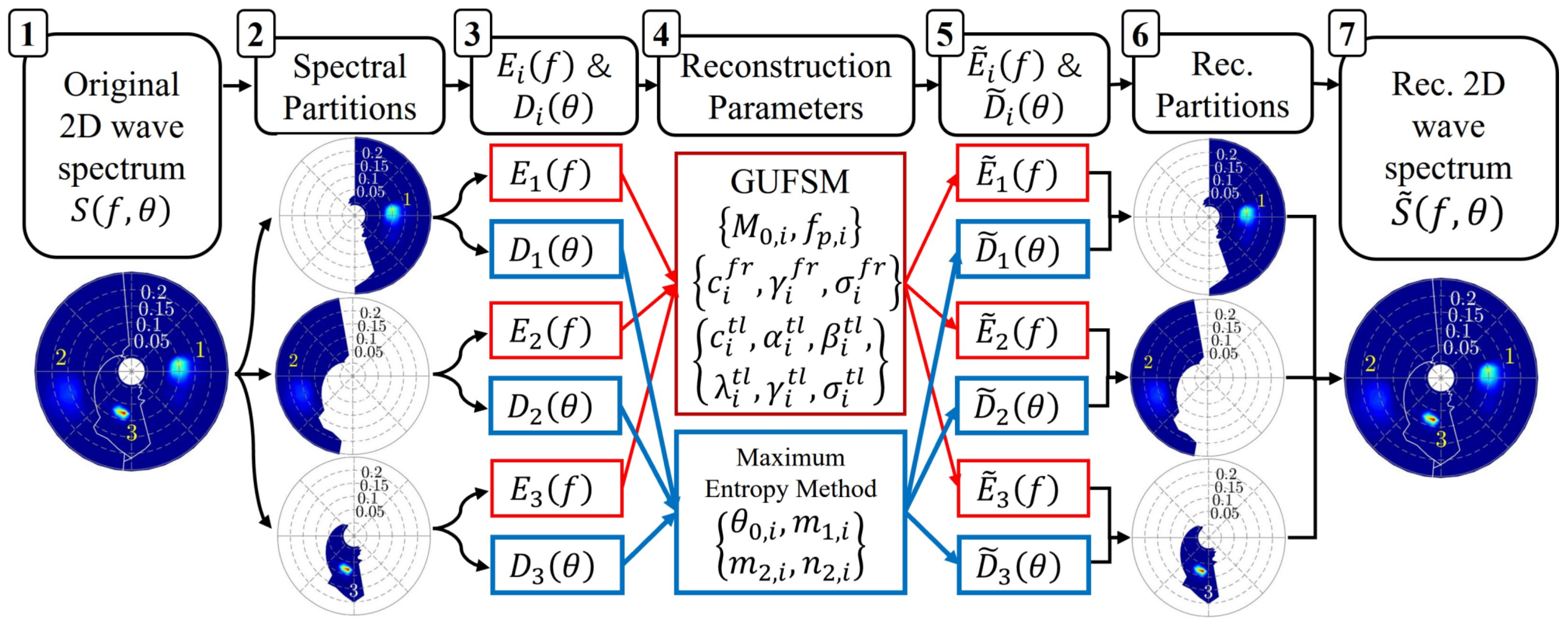
This paper presents a new approach for the preservation of 2D wave spectra. By introducing what are known as the Reconstruction Parameters (RPs), only dozens of storage units are needed to preserve a certain 2D spectrum. In conjunction with a corresponding reconstruction method, the spectra can then be rebuilt with intact spectral features. Experimental application confirmed that the reconstructed spectra could be adopted as boundary conditions in nested wave simulations.

The remainder of this paper is organized as follows. The steps of the proposed approach for the preservation and reconstruction of 2D wave spectra are presented in Section 2, together with the settings used in the application experiments. Section 3 provides comparisons between the original and reconstructed spectra and between the simulated results taking the two types of spectra as boundary conditions. Finally, a discussion and the derived conclusions are presented in Section 4 and Section 5, respectively.

2. Materials and Methods

2.1. Approach for Preservation and Reconstruction of 2D Wave Spectra

Figure 1 illustrates the basic steps of the proposed approach for the preservation and reconstruction of 2D wave spectra taking a spectrum with three wave systems (partitions) as an example.

First, a spectral partition (SP) technique is employed to separate the entire spectrum $S\left(f,\theta \right)$ into several partitions $S_i\left(f,\theta \right)$.

$$S\left(f,\theta \right)=\sum S_i\left(f,\theta \right).$$

(1)

The SP can be traced back to a digital image processing watershed algorithm [29], which can be applied to identify watershed lines, mountain peaks, and valleys in topographic maps. Because the 2D spectrum resembles a topological surface, applying such an algorithm in this circumstance is logical [30]. Partitioning of wave spectra is widely conducted in research concerning topics such as data assimilation [30,31,32] and the spatiotemporal tracking of wave systems [33,34]. The partitioning and identification program implemented in this work was developed based on the W3PARTMD module of the WaveWatch III model ver. 6.07 [35], in which an efficient FORTRAN routine was transformed from the MATLAB code [36,37] that was used to apply the watershed algorithm [29].

Particularly, the SP procedure can ensure that only one spectral peak is comprised in each partition. As shown in Figure 1, the frequency–directional ($f$–$\theta )$ spectral domain of the example spectrum is demonstrated in polar coordinates, and the spectral density is indicated by the colors. Three partitions are identified and labeled 1–3, and the boundaries are depicted by white lines.

Then, the one-dimensional (1D) frequency spectrum $E_i\left(f\right)$ and the directional distribution $D_i\left(\theta \right)$ can be obtained by integrating each partition $S_i$ along the frequency and the direction dimension, respectively:

$$E_i\left(f\right)={{\displaystyle \int }}_0^{2\pi }{S}_i\left(f,\theta \right)d\theta ,$$

(2)

$$D_i\left(\theta \right)=\frac{{{\displaystyle \int }}_0^{\infty }{S}_i\left(f,\theta \right)df}{M_{0,i}},$$

(3)

where the spectral moment $M_{0,i}={{\displaystyle \int }}_0^{\infty }{E}_i\left(f\right)df$, and it is noted that ${{\displaystyle \int }}_0^{2\pi }{D}_i\left(\theta \right)d\theta =1$. The peak frequency $f_{p,i}$ is determined as the frequency bin corresponding to $max\left(E_i\right)$.

The General Unimodal Frequency Spectrum Model (GUFSM), expressed as follows:

$$G\left(f\right)=c{\left(\frac{f}{f_p}\right)}^{-\alpha }{e}^{-\mathsf{\lambda }{\left(\frac{f}{f_p}\right)}^{-\beta }}{\gamma }^{\exp }\left(-\frac{{\left(1-\frac{f}{f_p}\right)}^2}{2{\sigma }^2}\right),$$

(4)

is proposed to represent the shape of $E_i\left(f\right)$. Using the least square method (LSM), the candidate RPs, such as $c$, $\alpha$, $\beta$, $\mathsf{\lambda }$, $\gamma$, and $\sigma$, can be adjusted to allow Equation (4) to fit the arbitrary $E_i\left(f\right)$. Furthermore, to obtain better goodness of fit and to reduce the number of RPs, $E_i\left(f\right)$ is divided into two parts, denoted as $E_i^{fr}$ and $E_i^{tl}$, based on the peak frequency $f_{p,i}$. For the front part $E_i^{fr}$, parameters $\alpha =5$, $\beta =4$, and $\lambda =1.25$ are fixed, and the undetermined RPs are ${\gamma }_i^{fr}$, ${\sigma }_i^{fr}$, and $c_i^{fr}$; however, considering the complex spectral shape at higher frequencies, all six RPs, denoted as $c_i^{tl}$, ${\alpha }_i^{tl}$, ${\beta }_i^{tl}$, ${\lambda }_i^{tl}$, ${\gamma }_i^{tl}$, and ${\sigma }_i^{tl}$, are involved in the tail part $E_i^{tl}$ LSM fitting processes. Therefore, the number of RPs for $E_i^{fr}$ and $E_i^{tl}$ are $n^{fr}=3$ and $n^{tl}=6$, respectively. Further details regarding the choices of $n^{fr}$ and $n^{tl}$ are discussed in Section 4.

Once the RPs for $E_i\left(f\right)$ are obtained, the parameters $c_i^{fr}$ and $c_i^{tl}$ need further rescaling as follows:

$$c_i^{fr}={\widehat{c}}_i^{fr}\frac{{{\displaystyle \int }}_0^{f_{p,i}}{E}_i^{fr}\left(f\right)df}{{{\displaystyle \int }}_0^{f_{p,i}}{\widehat{E}}_i^{fr}\left(f\right)df}, c_i^{tl}={\widehat{c}}_i^{tl}\frac{{{\displaystyle \int }}_{f_{p,i}}^{\infty }{E}_i^{tl}\left(f\right)df}{{{\displaystyle \int }}_{f_{p,i}}^{\infty }{\widehat{E}}_i^{tl}\left(f\right)df},$$

(5)

where ${\widehat{c}}_i^{fr}$ and ${\widehat{c}}_i^{tl}$ are the immediate outcomes of the LSM fitting, and ${\widehat{E}}_i^{fr}$ and ${\widehat{E}}_i^{tl}$ are the results of the GUFSM with substitutions of $\left\{{\widehat{c}}_i^{fr},{\gamma }_i^{fr},{\sigma }_i^{fr}\right\}$ and $\left\{{\widehat{c}}_i^{tl},{\alpha }_i^{tl},{\beta }_i^{tl},{\mathsf{\lambda }}_i^{tl},{\gamma }_i^{tl},{\sigma }_i^{tl}\right\}$, respectively. Notably, the other RPs of $E_i\left(f\right)$ do not need any rescaling.

The RPs for $D_i\left(\theta \right)$ are designed as follows:

$${\theta }_{0,i}={\tan }^{-1}\left(\frac{b}{a}\right) \mathrm{with} \{\begin{array}{c}a={{\displaystyle \int }}_0^{2\pi }\cos \left(\theta \right)D_i\left(\theta \right)d\theta \hfill \\ b={{\displaystyle \int }}_0^{2\pi }\sin \left(\theta \right)D_i\left(\theta \right)d\theta \hfill \end{array},$$

(6)

$$m_{1,i}={{\displaystyle \int }}_0^{2\pi }\cos \left(\theta -{\theta }_{0,i}\right)D_i\left(\theta \right)d\theta ,$$

(7)

$$m_{2,i}={{\displaystyle \int }}_0^{2\pi }\cos \left\{2\left(\theta -{\theta }_{0,i}\right)\right\}{D}_i\left(\theta \right)d\theta ,$$

(8)

$$n_{2,i}={{\displaystyle \int }}_0^{2\pi }\sin \left\{2\left(\theta -{\theta }_{0,i}\right)\right\}{D}_i\left(\theta \right)d\theta ,$$

(9)

and ${\theta }_{0,i}$ is also known as the mean direction of $D_i\left(\theta \right)$, and $m_{1,i}$, $m_{2,i}$, and $n_{2,i}$ are the so-called centered Fourier coefficients [38]. Therefore, the number of RPs for $D_i\left(\theta \right)$ is $n^{dr}=4$.

On the basis of the previously mentioned 15 RPs: $\left\{M_{0,i},f_{p,i},c_i^{fr},{\gamma }_i^{fr},{\sigma }_i^{fr},c_i^{tl},{\alpha }_i^{tl},{\beta }_i^{tl},{\mathsf{\lambda }}_i^{tl},{\gamma }_i^{tl},{\sigma }_i^{tl},{\theta }_{0,i},m_{1,i},m_{2,i},n_{2,i}\right\}$, each partition in the original 2D spectrum can then be reconstructed. Apparently, by substituting $\left\{c_i^{fr},{\gamma }_i^{fr},{\sigma }_i^{fr}\right\}$ and $\left\{{\alpha }_i^{tl},{\beta }_i^{tl},{\mathsf{\lambda }}_i^{tl},{\gamma }_i^{tl},{\sigma }_i^{tl}\right\}$ into Equation (4), the reconstructed ${\check{E}}_i^{fr}\left(f\in \left[0,f_{p,i}\right]\right)$ and ${\check{E}}_i^{tl}\left(f\in \left[f_{p,i},\infty \right]\right)$ can be obtained immediately. By combining the two parts mentioned above, we can obtain the first guess of ${\check{E}}_i\left(f\in \left[0,\infty \right]\right)$, in which ${\check{E}}_i\left(f_{p,i}\right)=max\left({\check{E}}_i^{fr}\left(f_{p,i}\right),{\check{E}}_i^{tl}\left(f_{p,i}\right)\right)$. Finally, the reconstructed 1D frequency spectrum for each partition can be expressed as follows:

$${\tilde{E}}_i\left(f\right)={\check{E}}_i\left(f\right)\frac{M_{0,i}}{{{\displaystyle \int }}_0^{\infty }{\check{E}}_i\left(f\right)df}$$

(10)

To reconstruct directional distributions, the Maximum Entropy Method [28,38] is employed. The first guess of the directional distribution of a certain partition is expressed as follows:

$$c_1=m_{1,i}{e}^{-j{\theta }_{0,i}},$$

(11)

$$c_2=\left(m_{2,i}-j{n}_{2,i}\right)e^{-2j{\theta }_{0,i}},$$

(12)

$${\varphi }_1=\frac{c_1-c_1^{*}{c}_2}{1-m_{1,i}^2},$$

(13)

$${\varphi }_1=\frac{c_1-c_1^{*}{c}_2}{1-m_{1,i}^2},$$

(14)

$${\check{D}}_i\left(\theta \right)=\frac{1}{2\pi }\frac{1-{\varphi }_1{c}_1^{*}-{\varphi }_2{c}_2^{*}}{{\left|1-{\varphi }_1{e}^{i\theta }-{\varphi }_2{e}^{2i\theta }\right|}^2},$$

(15)

where the asterisk denotes the complex conjugate, and we define $j^2=-1$. Finally, we set the following:

$${\tilde{D}}_i\left(\theta \right)=\frac{{\check{D}}_i\left(\theta \right)}{{{\displaystyle \int }}_0^{2\pi }{\check{D}}_i\left(\theta \right)d\theta },$$

(16)

to ensure that ${{\displaystyle \int }}_0^{2\pi }{\tilde{D}}_i\left(\theta \right)d\theta =1$.

The 2D wave spectral partitions can then be established as follows:

$${\tilde{S}}_i\left(f,\theta \right)={\tilde{E}}_i\left(f\right)\times {\tilde{D}}_i\left(\theta \right),$$

(17)

and the entire reconstructed spectrum can be reconstructed:

$$\tilde{S}\left(f,\theta \right)=\sum {\tilde{S}}_i\left(f,\theta \right).$$

(18)

2.2. Application of Reconstructed Spectra to Boundary Conditions in Nested Wave Modeling

The approaches established above can be applied to the boundary conditions in nested wave modeling by preserving the RPs on the boundaries when the parent model is running and by reconstructing the 2D spectra for boundary conditions when simulation using the child model is being conducted.

To demonstrate the application, wave field simulations were conducted using a pair of nested wave models for the Wanning offshore area (Hainan Island, China), including one parent simulation that provided the boundary conditions and two nested child simulations that separately used the original and reconstructed boundaries. The WaveWatch III [19,39] model ver. 6.07 [35] was employed as the parent model, covering the computational region of 5°S–45°N, 100°–150°E with 1/16° × 1/16° horizontal resolution. The child model adopted was the SWAN model ver. 41.41 [21,22], whose simulation domain covered the region of 18.5°–19.5°N, 110°–111°E with 1/20° × 1/20° rectangular grids.

Figure 2 shows the child computational domain, in which the 43 black circles along the sides denote the locations of the boundary points at which the boundary spectra are preserved and reconstructed. The intervals between the boundary points are 1/20°, and four of them, presented as red and denoted B1–B4, are selected as check points for comparison of the original and reconstructed spectra (see Section 3). Similarly, the yellow ‘+’ symbols denoted O1–O3 in Figure 2 are selected to confirm whether the statistics of the spectra simulated with reconstructed boundaries match those modeled with the original boundaries (also presented in Section 3). The locations of the check points are listed in

Table 1. Locations of check points.

Check Points	Latitude (degr. N)	Longitude (degr. E)	Depth (m)
B1	18.5	110.5	88
B2	18.5	111.0	171
B3	19.0	111.0	96
B4	19.5	111.0	41
O1	19.0	110.8	71
O2	18.6	110.6	97
O3	19.0	110.6	26

.

The simulated spectral space in both the parent and the child models was set with 36 directions at intervals of 10° and at 35 frequencies spaced from 0.042 to 1.07 Hz as a geometric progression with a ratio of 1.1. Therefore, in this study, storing a 2D spectrum at a certain original boundary point required 35 × 36 = 1260 storage units, which is a value typical of current wave modeling research.

In practice, it is unnecessary to involve all the original identified spectral partitions in Equation (18) because partitions with very low wave energy can be spurious partitions or noise that might interfere with the main features of the original spectra. In this study, partitions with a value of $4\sqrt{M_{0,i}}<0.05$ (the significant wave height of the partition is smaller than 0.05 m) were ignored; and the maximum number of partitions involved in the reconstruction was set at four, with candidate partitions ordered from large to small based on their respective $M_{0,i}$ values. Further discussion on the setting of the maximum number is presented in Section 4. Therefore, through the proposed preservation approach, the number of storage units occupied to save the RPs of a 2D spectrum is reduced to a maximum of 15 × 4 = 60.

The period of the simulations was the year 2018, and the spectra and RPs on the boundary points were preserved and reconstructed hourly. Both child simulations were conducted with the exact same model settings, including source terms representing the effects of nonlinear quadruplet wave interactions [40,41], wind input [42,43], white capping [43], swell dissipation [44], depth-induced wave breaking [45], bottom friction [25], and triad wave–wave interactions [46]. The wind force adopted in the simulations was derived from ECMWF-ERA5 analysis hourly data [15], which provided the u–v wind field at the height of 10 m above the sea surface with 0.25° × 0.25° horizontal resolution. Bathymetric data were obtained from the ETOPO1 model of the U.S. National Geophysical Data Center [47].

3. Results

To validate the newly proposed approach and its application in wave modeling, three sets of comparisons are presented in this section, including comparisons of the original and reconstructed spectra/partitions at boundary points, of SWAN field outputs simulated with original and reconstructed boundaries, and of spectral statistics derived from the two field outputs mentioned above.

Table 2. KPs adopted to represent the characteristics of spectra and partitions.

KPs	Definition and Calculation
$H_{m0}$	Significant wave height, denoted as $H_{m0}$ in meters, is calculated as follows:
	$H_{m0}=4\sqrt{m_0}$
	where the spectral moment of order n is calculated as
	$m_{ n}={{\displaystyle \int }}_{ 0}^{ \infty }{f}^{ n} E\left(f\right) df$
$T_{m01}$	Mean wave period based on first moment, denoted as $T_{m01}$ in seconds, is calculated as follows:
	$T_{m01}=\frac{m_0}{m_1}$
$T_{m02}$	Mean wave period based on second moment, also known as mean zero-crossing wave period (in seconds), is calculated as follows:
	$T_{m02}=\sqrt{\frac{m_0}{m_2}}$
$T_e$	Mean wave period based on the moment of order −1, also known as wave energy period (in seconds), is calculated as follows:
	$T_e=\frac{m_{-1}}{m_0}$
$f_p$	Peak frequency $f_p$ (in $Hz$) is determined as the frequency bin corresponding to the maximum value of $E\left(f\right)$.
$T_p$	Peak wave period (in seconds) is calculated as $T_p=\frac{1}{f_p}$.
$E\left(f_p\right)$	Peak spectral density (in $m^{2}s$), i.e., the maximum value of $E\left(f\right)$.
$WPD$	Wave power density [48] characterizes the time-averaged energy flux through an envisioned vertical cylinder of unit diameter; its unit is usually taken as kW/m (kilowatts per meter) or $m^3/s$. This parameter can be estimated as follows:
	$WPD=\rho g{{\displaystyle \int }}_0^{\infty }{C}_{g}E\left(f\right)df$
	$WP{D}_x=\rho g{{\displaystyle \int }}_0^{\infty }{C}_{g,x}E\left(f\right)df$
	$WP{D}_y=\rho g{{\displaystyle \int }}_0^{\infty }{C}_{g,y}E\left(f\right)df$
	where $\rho =1023 kg/m^3$ denotes the density of seawater, $g=9.81 m/s^2$ is the acceleration of gravity, and
	$c_g=\frac{2\pi f}{k}\left(1+\frac{2kd}{sinh\left(2kd\right)}\right)$
	is the group velocity which is associated with the water depth $d$ and wave number $k$.
$WLEN$	Mean wavelength (in meters) is defined as
	$WLEN=2\pi {\left(\frac{{{\displaystyle \int }}_0^{\infty }kE\left(f\right)df}{m_0}\right)}^{-1}$
	where $k$ denotes wave number.
$Q_p$	The peakedness of the wave spectrum [49] (non-dimensional), defined as follows:
	$Q_p=2\frac{{{\displaystyle \int }}_0^{\infty }f{E}^2\left(f\right)df}{m_0^2}$
	A smaller value of $Q_p$ indicates a wider spectrum.
$FSPR$	The normalized frequency width of the spectrum (frequency spreading) is defined as [50]:
	$FSPR=\frac{\left|{{\displaystyle \int }}_0^{\infty }E\left(f\right)e^{j2\pi f\tau }df\right|}{m_0}$
	Where $\tau =T_{m02}$ and $j=\sqrt{-1}$.
${\theta }_0$ (${\theta }_{0,x}$ & ${\theta }_{0,y})$	Mean wave direction (in degr. and Nautical convention) is calculated as
	${\theta }_0={\tan }^{-1}\left(b/a\right)$
	where $a={{\displaystyle \int }}_0^{2\pi }\cos \theta D\left(\theta \right)d\theta$ and $b={{\displaystyle \int }}_0^{2\pi }\sin \theta D\left(\theta \right)d\theta$ and the x and y components of ${\theta }_0$ can be expressed as: ${\theta }_{0,x}=\cos \left({\theta }_0\right)$ and ${\theta }_{0,y}=\sin \left({\theta }_0\right)$.
${\sigma }_{\theta }$	The one-side directional width of the spectrum (directional spreading or directional standard deviation, in degr.) is defined as [38]
	${\sigma }_{\theta }={\left\{2\left[1-{\left(\frac{a^2+b^2}{m_0^2}\right)}^{1/2}\right]\right\}}^{1/2}$

lists some of the Key Parameters (KPs) that can represent the characteristics of spectra and partitions. Moreover, we introduce Pearson’s correlation coefficient (R):

$$\mathrm{R}=\frac{{\sum }_i((R{E}_i-\overline{RE})(O{R}_i-\overline{OR}))}{\sqrt{{\sum }_i(R{E}_i-\overline{RE}{)}^2·{\sum }_i(O{R}_i-\overline{OR}{)}^2}},$$

(19)

and the mean absolute error (MAE):

$$\mathrm{MAE}=\frac{1}{N}{\sum }_{i=1}^N|R{E}_i-O{R}_i|,$$

(20)

to indicate the quantitative errors between the comparison objects. In Equations (19) and (20), $RE$ and $OR$ denote the KPs obtained based on the reconstructed and the original spectra/partitions, respectively, subscript $i$ indicates the index of each sample, $N$ is the total number of samples, and $\overline{RE}=\frac{1}{N}{\sum }_{i=1}^{N}R{E}_i,$ and $\overline{OR}=\frac{1}{N}{\sum }_{i=1}^{N}O{R}_i,$.

3.1. Comparison between Original and Reconstructed Spectra/Partitions at Boundary Points

Figure 3 shows the scatter plots of the KPs derived at check point B2. In each panel, the x (y) axis indicates the values of a specific KP obtained from the original (reconstructed) partitions, and the name of the KP can be found in the title. The partitions from the same spectrum have been ordered from large to small based on their $H_{m0}$ value; therefore, each member of “Part1” exhibited in Figure 3a is the partition with the largest $H_{m0}$ value in each sampling spectrum; similarly, Part2 to Part4 in Figure 3b–d, respectively, refer to the second to fourth largest partitions. Figure 4 presents comparisons of the entire spectra, and the reconstructed spectra are rebuilt with the four largest partitions; the scatter plots shown in Figure 4 are the same as those in Figure 3. The corresponding R and MAE values for both the partitions (Part1–6) and the entire spectra (Part0) are exhibited in

Table 3. Correlation coefficient (R) of the KPs derived from the original and the reconstructed spectra/partitions at check point B2. Sample numbers of Part0 to Part6 are 8760, 6407, 8729, 3295, 1483, 449, and 97, respectively.

	KPs	${\mathit{H}}_{\mathit{m}0}$	${\mathit{f}}_{\mathit{p}}$	${\mathit{T}}_{\mathit{m}01}$	${\mathit{T}}_{\mathit{m}02}$	${\mathit{T}}_{\mathit{e}}$	$\mathit{W}\mathit{P}\mathit{D}$	$\mathit{W}\mathit{L}\mathit{E}\mathit{N}$	$\mathit{E}\left({\mathit{f}}_{\mathit{p}}\right)$	${\mathit{Q}}_{\mathit{p}}$	$\mathit{F}\mathit{S}\mathit{P}\mathit{R}$	${\mathit{\theta }}_{0,\mathit{x}}$	${\mathit{\theta }}_{0,\mathit{y}}$	${\mathit{\sigma }}_{\mathit{\theta }}$
Partn
Part0		1.000	0.961	0.986	0.955	0.999	1.000	0.930	0.999	0.970	0.972	1.000	0.999	0.995
Part1		1.000	1.000	0.990	0.973	0.999	1.000	0.973	0.999	0.977	0.957	1.000	0.999	0.990
Part2		1.000	1.000	0.996	0.993	0.999	1.000	0.991	0.999	0.985	0.973	0.998	0.996	0.982
Part3		1.000	1.000	0.999	0.997	0.999	1.000	0.998	0.999	0.979	0.962	0.994	0.997	0.929
Part4		1.000	1.000	0.999	0.998	1.000	1.000	0.999	1.000	0.970	0.936	0.994	0.991	0.925
Part5		1.000	1.000	0.999	0.999	1.000	1.000	0.999	0.999	0.961	0.926	0.994	0.986	0.904
Part6		1.000	1.000	0.999	0.999	0.999	1.000	0.999	0.996	0.961	0.923	0.997	0.996	0.857

and

Table 4. Mean absolute error (MAE) of the KPs derived from the original and the reconstructed spectra/partitions at check point B2. Sample numbers of Part0 to Part6 are 8760, 6407, 8729, 3295, 1483, 449, and 97, respectively.

	KPs	${\mathit{H}}_{\mathit{m}0}$ $\left(\mathbf{m}\right)$	${\mathit{f}}_{\mathit{p}}$  $\left(\mathbf{Hz}\right)$	${\mathit{T}}_{\mathit{m}01}$  $\left(\mathbf{s}\right)$	${\mathit{T}}_{\mathit{m}02}$  $\left(\mathbf{s}\right)$	${\mathit{T}}_{\mathit{e}}$  $\left(\mathbf{s}\right)$	$\mathit{W}\mathit{P}\mathit{D}$ $\left(\mathbf{k}\mathbf{W}/\mathbf{m}\right)$	$\mathit{W}\mathit{L}\mathit{E}\mathit{N}$  $\left(\mathbf{m}\right)$	$\mathit{E}\left({\mathit{f}}_{\mathit{p}}\right)$ $\left({\mathbf{m}}^2\mathbf{s}\right)$	${\mathit{Q}}_{\mathit{p}}$	$\mathit{F}\mathit{S}\mathit{P}\mathit{R}$	${\mathit{\theta }}_0$ $\left(\mathit{d}\mathit{e}\mathit{g}\mathit{r}.\right)$	${\mathit{\sigma }}_{\mathit{\theta }}$ $\left(\mathit{d}\mathit{e}\mathit{g}\mathit{r}.\right)$
Partn
Part0		0	0.0012	0.16	0.25	0.06	0.12	4.3	0.0958	0.0504	0.0167	0.8	0.6094
Part1		0	0.0002	0.17	0.27	0.06	0.09	4.8	0.0779	0.0676	0.0179	0.9	0.552
Part2		0	0.0001	0.13	0.2	0.06	0.05	4.2	0.0456	0.2108	0.028	2.2	1.1075
Part3		0	0.0001	0.11	0.15	0.07	0	3.6	0.0054	0.353	0.0355	3.6	1.5116
Part4		0	0	0.09	0.12	0.06	0	3.3	0.0027	0.5448	0.0409	3.4	1.3202
Part5		0	0	0.09	0.12	0.06	0	3.7	0.0018	0.4985	0.037	2.9	1.2933
Part6		0	0.0002	0.09	0.11	0.07	0	3.8	0.0017	0.477	0.0348	1.9	1.0665

, respectively. Notably, Part1–4 in the two tables can be referred to Figure 3a–d, and two more sets of partitions with smaller $H_{m0}$ values are also presented. Finally, the sample numbers of Part1–6 at B2 are 6407, 8729, 3295, 1483, 449, and 97; therefore, in most cases, the maximum number of coexisting wave systems at B2 is fewer than four.

From Figure 3 and Figure 4 and Table 3 and Table 4, the reconstructed $H_{m0}$, $f_p$, and the related $E\left(f_p\right)$, can be found to be almost entirely consistent with the originals, although the reconstructed $f_p$ in the entire spectra might sometimes deviate substantially from the original. In fact, $f_p$ is defined directly as the frequency corresponding to the maximum spectral density, which is meaningful in a unimodal spectrum, e.g., each partition identified in this study because most energy might concentrate at the frequency; however, it becomes meaningless in a spectrum where multiple wave systems (partitions) coexist.

The KPs representing wave periods, such as $T_{m01}$, $T_{m02}$, and especially $T_e$, are also reconstructed well, as shown in the above-mentioned figures and tables. In comparison with $T_e$, both $T_{m01}$ and $T_{m02}$ are more sensitive to the spectral shape in high-frequency bands owing to the higher order spectral moments that are involved. For developed waves with larger $H_{m0}$ and lower $f_p$, such as the waves in Part1 and Part2, the SP step introduced in the newly proposed approach might influence the spectral shapes in higher frequencies, causing greater deviation from the “normal” patterns that can be expressed by the GUFSM; similar spectral tails can also be observed in multimodal spectra. This is why poorer agreement for $T_{m01}$ and $T_{m02}$ can be found in reconstructed Part1 and Part2 and in the entire spectra than in Part3–6. Similar elucidation can also be performed on the reconstructed $WLEN$. Nevertheless, the quantitative errors for those KPs shown in Table 3 and Table 4 are acceptable.

Figure 3 and Figure 4 and Table 3 and Table 4 show that the mean wave direction ${\theta }_0$ can be effectively rebuilt in both the entire spectra and the spectral partitions. The same goodness of fit can also be found in the KPs of $WPD$, which implies that the new approach can be adopted in research associated with wave energy assessment. As for the KPs associated with spectral width, e.g., $Q_p$, $FSPR$, and ${\sigma }_{\theta }$, the newly proposed approach can produce better reconstruction results for the entire spectra, but the agreements might become poorer for partitions with smaller values of $H_{m0}$.

The comparison results for the partitions and spectra at check points B1 (Figures S1 and S2 and Tables S1 and S2), B3 (Figures S3 and S4 and Tables S3 and S4), and B4 (Figures S5 and S6 and Tables S5 and S6) are similar to those at B2, and the relevant figures and tables can be found in the Supplementary Material. We can then conclude that a certain 2D spectrum occupying 1260 storage units can be preserved with the RPs requiring a maximum of 60 units, and reconstructed with intact key characteristics via the reconstruction approach proposed in this study.

3.2. Comparison of SWAN Field Outputs

The spatial distributions of the coefficients R and MAE for the modeled wave fields are illustrated in Figure 5 and Figure 6, respectively. The coefficients mentioned above were derived from the SWAN BLOCK outputs covering the entire nested domain. In each panel of Figure 5 (6), the colors indicate the values of R (MAE), the title identifies the corresponding KP, and the x and y axes denote longitude (°E) and latitude (°N), respectively. Notably, the KPs’ outputs by the SWAN model were calculated using the entire simulated spectra, involving both wind-sea and swell contributions.

Figure 5 shows that for conventional wave parameters such as $H_{m0}$, $T_{m01}$, $T_{m02}$, $T_e$, $WLEN$, $WPD$ (here presented as $WP{D}_x$ and $WP{D}_y)$, and ${\theta }_0$ (here presented as ${\theta }_{0,x}$ and ${\theta }_{0,y})$, the simulated results with the original and the reconstructed boundaries can match strongly (R > 0.99) in most parts of the nested domain; and for the spectral width parameters, as well as parameter $T_p$, the results achieving a strong level of agreement (R > 0.95) can also cover the main part of the demonstration region. The spatial distribution of MAEs illustrated in Figure 6 further reveals that the simulation errors due to using the original and reconstructed boundaries can be far smaller than those occurring in the validation of wave modeling results against the observations. Apparently, the characteristics of the original spectra can be transferred to the nested wave fields through the reconstructed boundaries.

3.3. Comparion of Spectral Statistics

The modeled 2D spectra at check points O1–O3 shown in Figure 2 were retained during the simulations to further validate that the characteristics of the original partitions could also be transferred to the nested domain through the reconstructed boundary conditions.

The Two-step Spectral Partition procedure [51] is introduced to perform statistical analyses on these partitions. Because the peaks of the partitions, identified by the (first-step) SP procedure, could occur at any location in the $f–\theta$ spectral space, the probability of their occurrence then forms another 2D spectrum; by partitioning the newly formed spectrum (second-step partition), the identified partitions can then be grouped automatically. The statistics of the grouped partitions over a long time series can reflect physical reality and have climatic significance [51,52,53].

The partition groups identified at check point O1 are illustrated in Figure 7, where the $f–\theta$ spectral space is presented in polar coordinates, as in Figure 1, but where the colors in Figure 7 indicate the number of peak occurrences in the $f–\theta$ cells. At least seven groups are identified for the spectrum series derived separately from the original and the reconstructed boundary forcing simulations, and those groups are labeled 1–7 and ordered from large to small based on the peak-occurrence numbers, and the boundaries of the groups are depicted by the white lines.

Figure 7a shows that the dominant wave systems simulated with the original boundaries at O1 are Grp-1 and Grp-2, which are concentrated in the direction ENE–E and S, respectively. Additionally, Figure 7b confirms that the spectra simulated with the reconstructed boundary conditions present the same prevailing wave systems at the same check points.

Probability distributions of the KPs derived from the partitions involved in Grp-1 and Grp-2 at O1 are illustrated in Figure 8 and Figure 9, respectively. The panels of the two figures are titled according to the corresponding KPs, the KP probability densities for the partitions simulated with the original and the reconstructed boundaries are indicated by solid lines and circles, respectively, and the x axis in each panel denotes the value range of the KP.

Figure 8 and Figure 9 show that the probability distributions of the KPs derived from the reconstructed boundary forcing wave field conform well with those obtained using the original boundary conditions in terms of both dominant wave system groups. Therefore, using the boundary conditions reproduced by the newly proposed approach, the climatological patterns of the original simulated wave fields, including both the prevailing wave systems and the probability distribution of the associated KPs, can be well retained, i.e., the wave characteristics of the original partitions can be successfully transferred to the nested wave fields through the reconstructed boundary conditions.

Comparisons of the spectral statistics at check points O2 (Figures S7, S9 and S10) and O3 (Figures S8, S11 and S12) reveal similar results, and the relevant figures can be found in the Supplementary Material. From the comparisons presented in Section 3.2 and Section 3.3, we can conclude that the newly proposed approach can be applied to nested wave simulations. Moreover, we can also infer that the boundary conditions preserved and reconstructed using the new approach can be adopted in research that relies on long-term wave statistics, e.g., safety design regarding engineering structures, wave climatology studies, and assessment of wave energy resources.

4. Discussion

This paper presents a new approach for preservation and reconstruction of 2D wave spectra, whereby the reconstructed spectra can be applied as boundary conditions in wave nested modeling. Typically, preservation of a 2D spectrum at a certain boundary point might occupy 35 × 36 = 1260 storage units; however, using the proposed approach the storage needed could be reduced to a maximum of 60 units.

As mentioned above, a parametric wave spectrum with an imposed directional distribution can also be used to reconstruct nesting boundaries, and only several parameters are needed in such a reconstruction. For example, 2D spectra can be reconstructed using the functional form of the TMA spectrum [54,55] with the Mitsuyasu-type [27] directional distribution. The TMA spectrum can be expressed as follows:

$$\left(f\right)=S_J\left(f\right)\varphi \left(kh\right),$$

(21)

where $S_J\left(f\right)$ denotes the functional form of the JONSWAP spectrum [25,56]:

$$S_J\left(f\right)={\beta }_J{H}_s^2\frac{f^{-5}}{f_p^{-4}}exp\left[-1.25{\left(\frac{f}{f_p}\right)}^{-4}\right]{\gamma }^{exp\left[\raisebox{1ex}{$-{\left(\frac{f}{f_p}-1\right)}^2$}\!\left/ \!\raisebox{-1ex}{$2{\sigma }^2$}\right.\right]},$$

(22)

$$\sigma =\left\{\begin{array}{c}0.07:f\le f_p\\ 0.09:f>f_p\end{array}\right.,$$

(23)

where $H_s$ denotes the significant wave height, $f_p$ indicates the peak frequency, $\gamma$ is the peakedness parameter, and ${\beta }_J\approx \frac{0.06238}{0.230 + 0.0336\gamma - 0.185{\left(1.9 + \gamma \right)}^{-1}}\left(1.094-0.01915\ln \gamma \right)$; in Equation (21), $\varphi \left(kh\right)$ [54] is a function related to the wave number $k$ and local water depth $h$ as follows:

$$\varphi \left(kh\right)=\frac{{\tanh }^{2}kh}{1+2kh/\sinh 2kh}$$

(24)

The Mitsuyasu-type directional distribution can be expressed as follows:

$$D\left(\theta \right)=A {\cos }^{2s}\left(\frac{\theta -{\theta }_p}{2}\right)$$

(25)

where $s$ controls the directional spreading, ${\theta }_p$ denotes the peak wave direction, i.e., the mean direction derived from the directional distribution at $f_p$, and $A$ is a scale factor to ensure that $\int D\left(\theta \right)d\theta =1$.

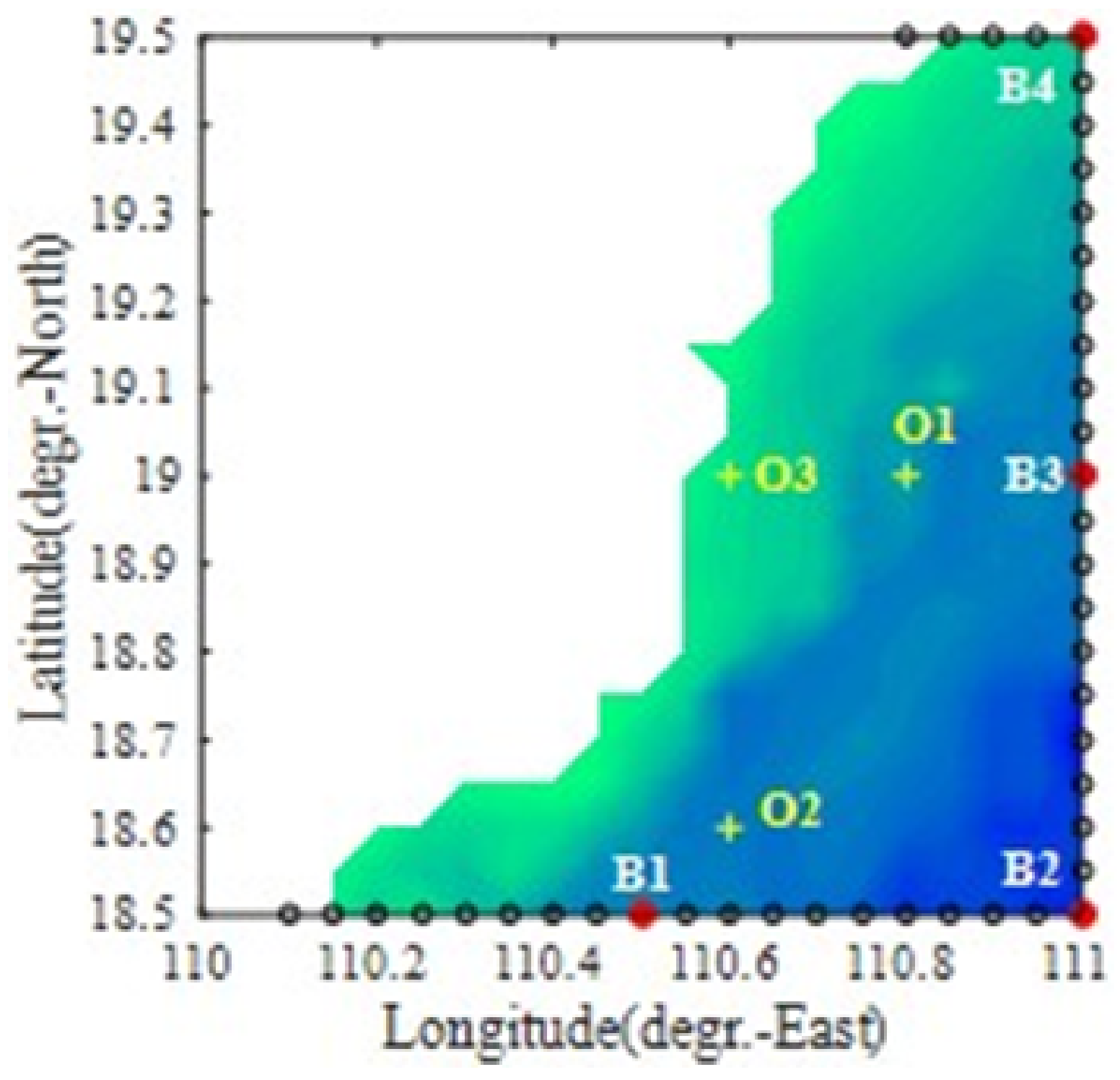
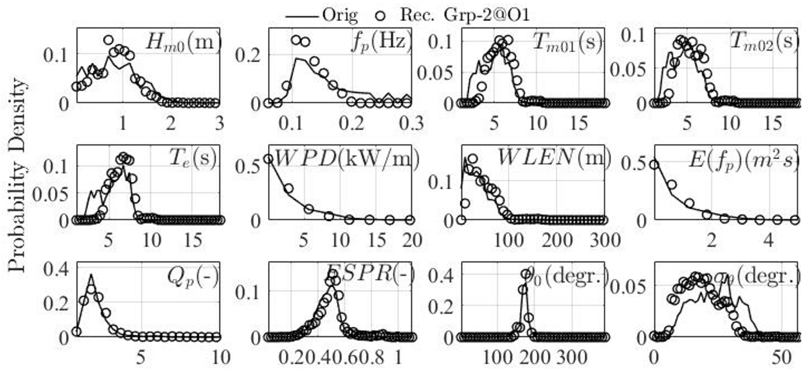
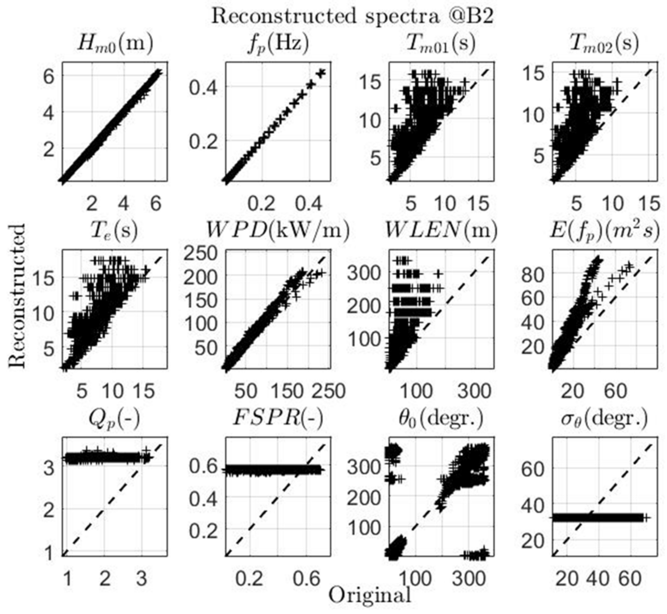
Figure 10 shows a comparison of the TMA–Mitsuyasu reconstructed and the original spectra at check point B2. For each reconstructed spectrum, the parameters needed are only $h$, $H_s$, $f_p$, and ${\theta }_0$, the latter three of which are calculated from the entire spectrum at the original boundaries, $h$ is read from the bathymetric data at B2, and $\gamma =3.3$ is set as a constant owing to the lack of available information. The scatter plots and KPs in Figure 10 are similarly arranged as those in Figure 3 and Figure 4.

Figure 10 shows that even though only four parameters are necessary in the reconstruction, the reconstructed spectra retain several features such as $H_{m0}$, $f_p$, and $WPD$, that have acceptable agreement with the originals. The reconstructed KPs associated with wave period, wavelength, and peak spectral density present greater deviation from the originals as their values increase, as well as the mean wave direction. Furthermore, the characteristics of spectral width are limited at a fixed value because of the lack of relevant information input. Similar results at the other check points (Figures S13–S15 for points B1, B3, and B4, respectively) on the boundaries can be found in the Supplementary Material.

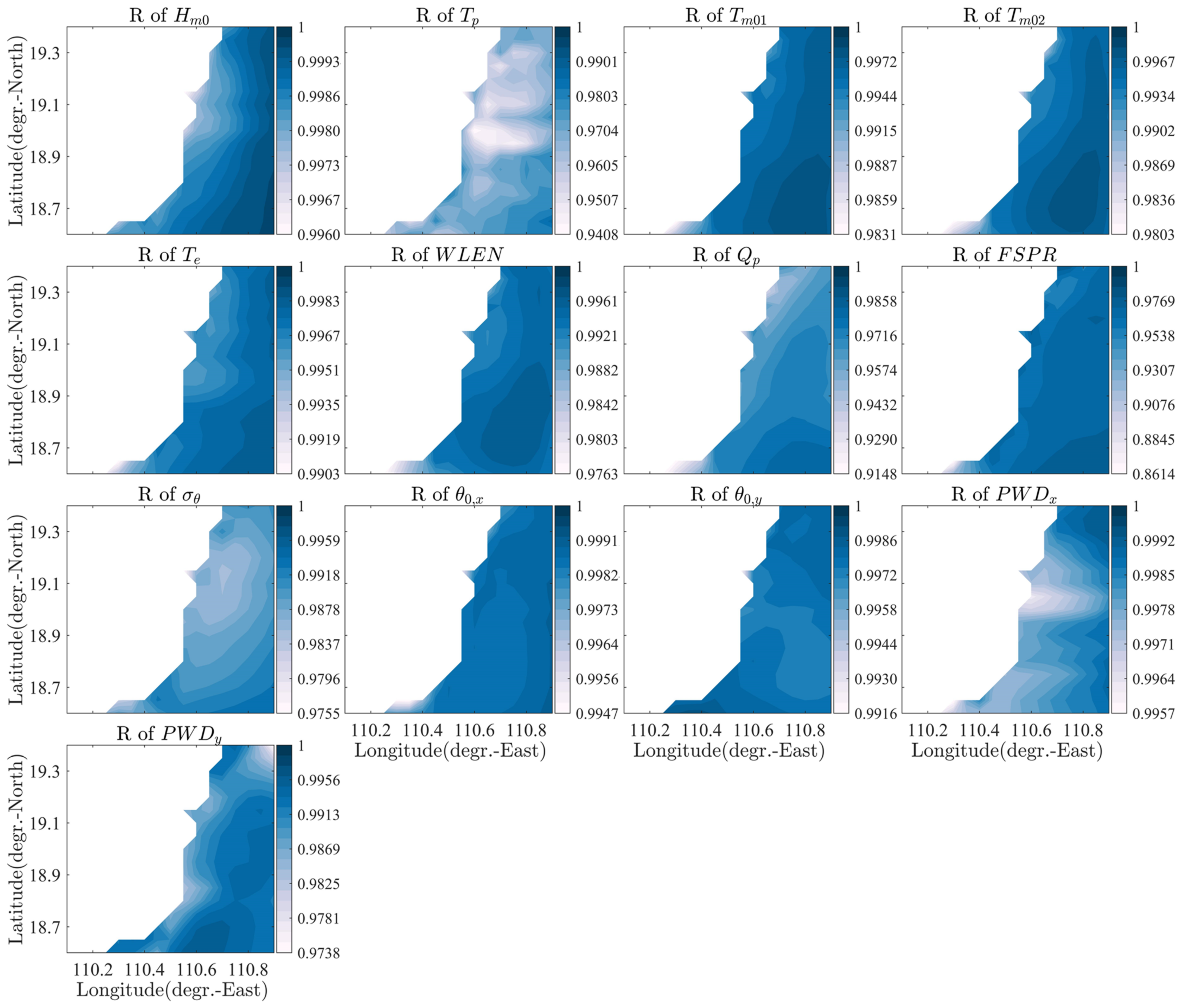
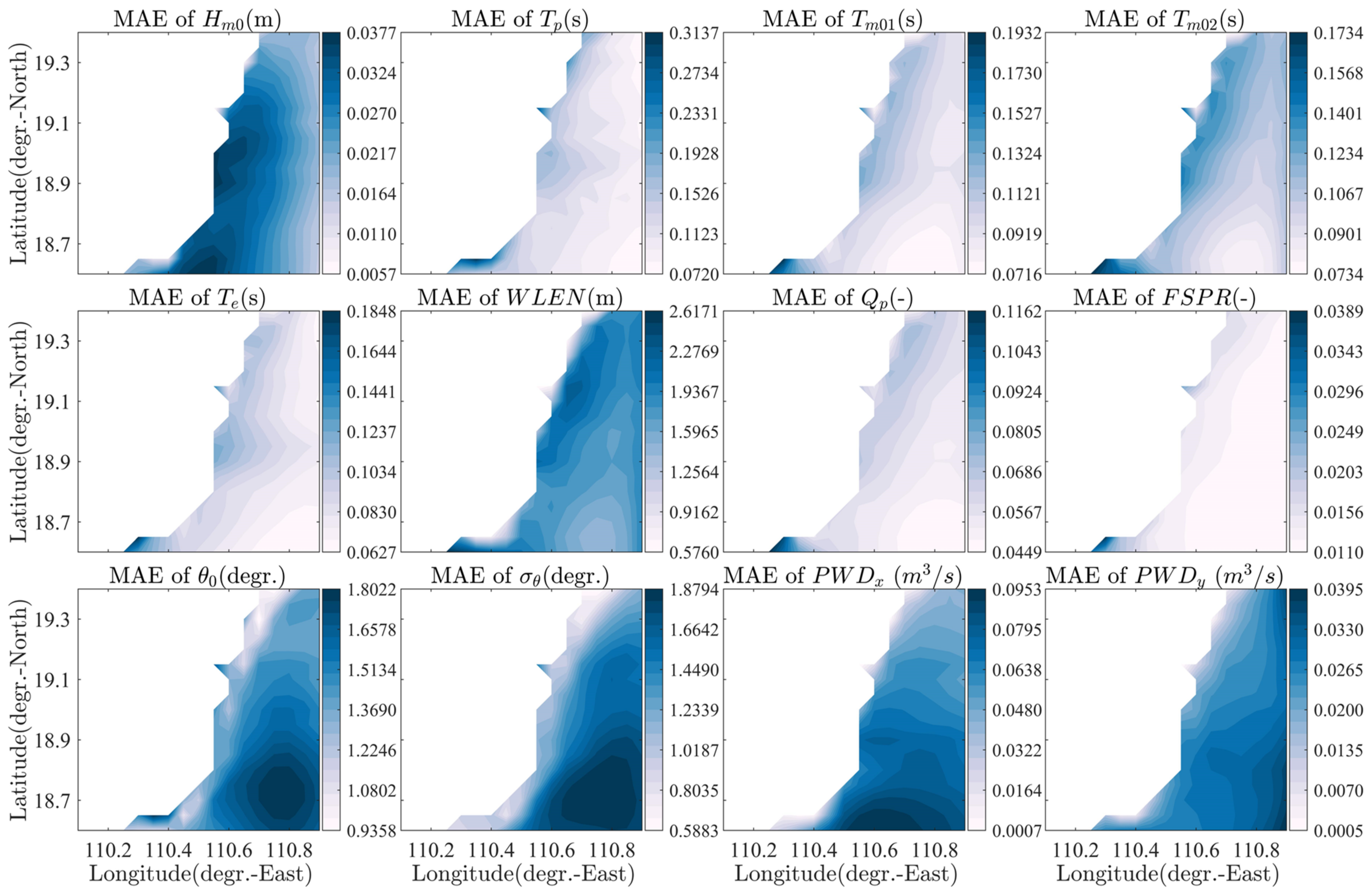
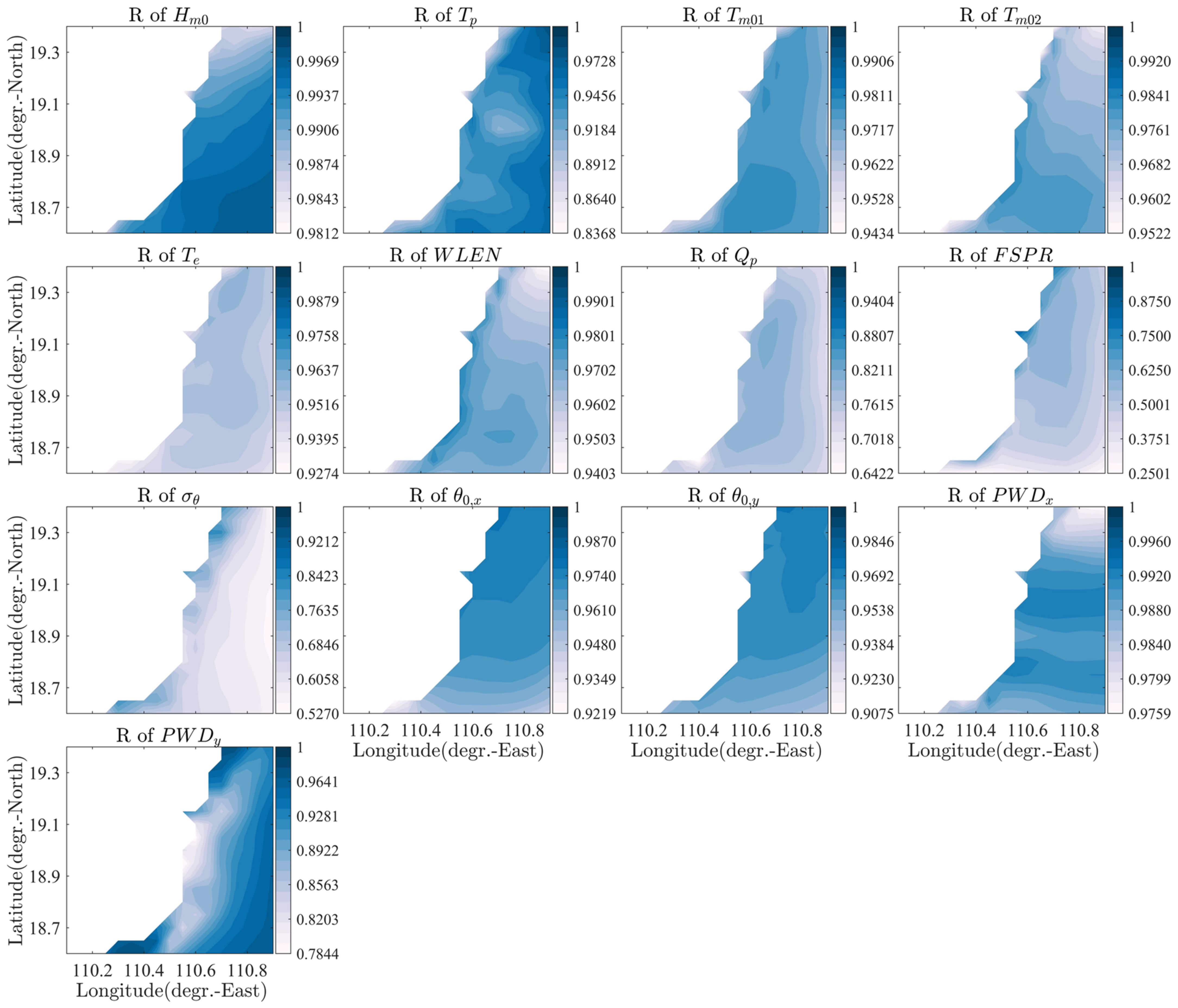
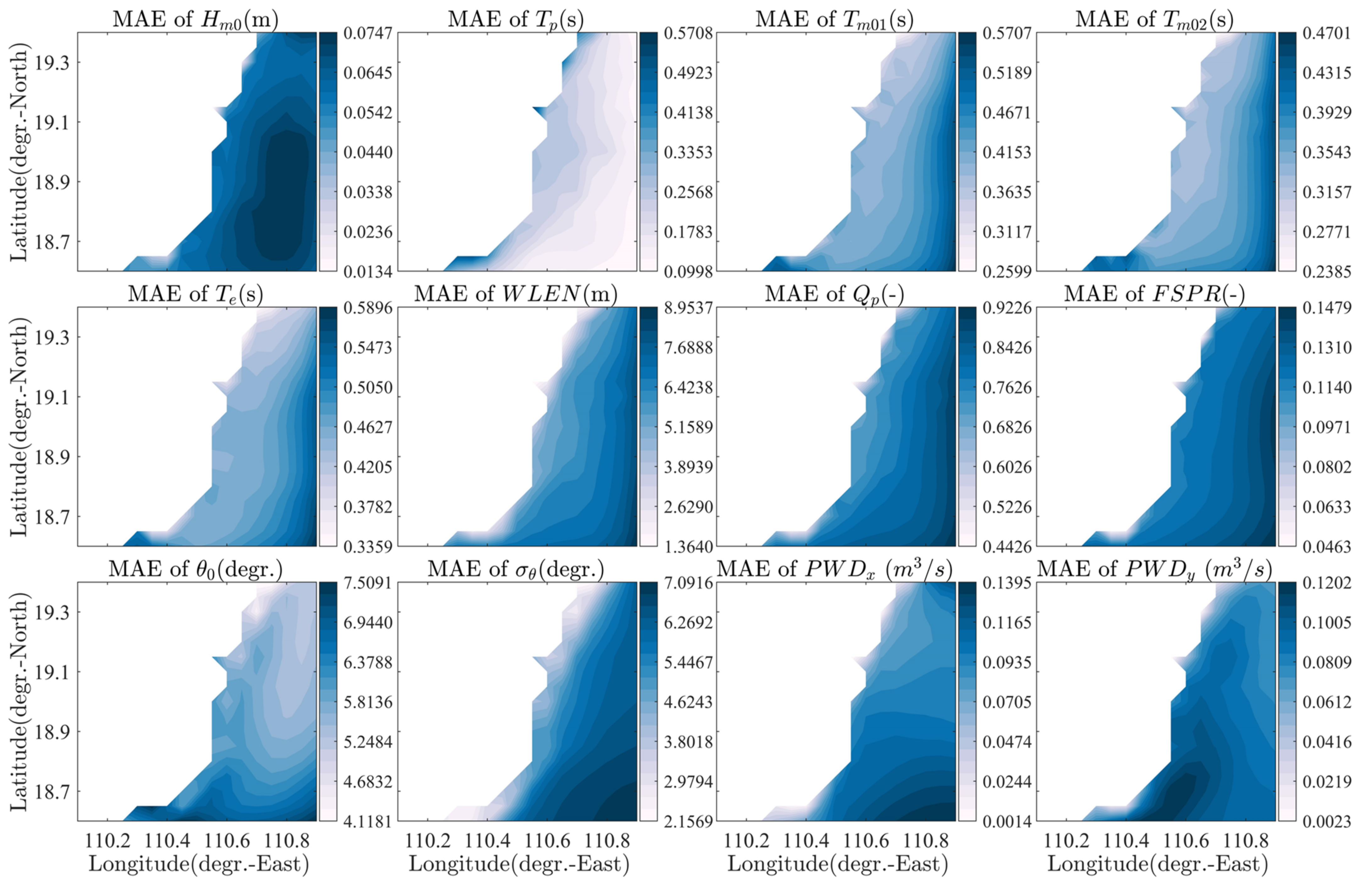
Figure 11 (12) demonstrates the similar spatial distribution of R (MAE) derived from the SWAN field output simulated with the original and the TMA–Mitsuyasu reconstructed boundaries. The colors, KPs, and demonstration region shown in Figure 11 and Figure 12 are the same as those shown in Figure 5 and Figure 6. In comparison with the results simulated using the boundaries reconstructed by the new approach, the quantitative errors illustrated in Figure 11 and Figure 12 reveal much poorer agreement with the original simulations. For example, the R values are reduced by approximately 10% and over 50% for the best and worst situations, respectively. The values of MAE also increase by approximately three to five times in comparison with those of the new approach, especially for the crucial features of wave height, period, and wave direction.

The key concept in the new approach is consideration of the spectral partitions as the fundamental units for preservation and reconstruction, which offers the following benefits: (i) each partition contains only one peak, making the spectral shape more convenient for processing, and (ii) partitions with low energy, as well as spurious partitions and noise, can be filtered, thereby making it easier to preserve and reconstruct the primary characteristics of the original spectra.

Technically, one of the key points is the adoption of the GUFSM in the LSM fittings, in addition to the separate fittings performed on the front and tail parts of the 1D frequency spectra. In the fitting step, determination of the number of RPs, i.e., $n^{fr}$ and $n^{tl}$, still deserves further discussion. The strategies for selecting $n$ can be enumerated as follows:

• $n=3$: $\alpha =5$, $\beta =4$, and $\lambda =1.25$ are fixed, and the RPs to be fitted are $\mathsf{\gamma }$, $\sigma$, and $c$;
• $n=4$: $\alpha =5$ and $\beta =4$ are fixed, and the RPs to be fitted are $\lambda$, $\mathsf{\gamma }$, $\sigma$, and $c$;
• $n=6$: the RPs to be fitted are $\alpha$, $\beta$, $\lambda$, $\mathsf{\gamma }$, $\sigma$, and $c$.

Table 5. Correlation coefficient (R) of the KPs derived from the original and the reconstructed (obtained under different strategies of $n^{fr}$ and $n^{tl}$ ) partitions at check point B2. The R values were derived from all the partitions identified, and the values illustrated under the other $n^{fr}$ and $n^{tl}$ combinations are relative to those obtained under the setting of $n^{fr}=3$ and $n^{tl}=6$.

	KPs	${\mathit{H}}_{\mathit{m}0}$	${\mathit{f}}_{\mathit{p}}$	${\mathit{T}}_{\mathit{m}01}$	${\mathit{T}}_{\mathit{m}02}$	${\mathit{T}}_{\mathit{e}}$	$\mathit{W}\mathit{P}\mathit{D}$	$\mathit{W}\mathit{L}\mathit{E}\mathit{N}$	$\mathit{E}\left({\mathit{f}}_{\mathit{p}}\right)$	${\mathit{Q}}_{\mathit{p}}$	$\mathit{F}\mathit{S}\mathit{P}\mathit{R}$
${\mathit{n}}^{\mathit{f}\mathit{r}}$$\& {\mathit{n}}^{\mathit{t}\mathit{l}}$
$n^{fr}=3,$ $n^{tl}=6$		1	0.9997	0.9969	0.9935	0.9993	0.9999	0.9943	0.9992	0.9864	0.9756
$n^{fr}=4,$ $n^{tl}=6$		0	−0.0005	0.0001	0.0001	0.0002	0	0.0001	0.0006	0.0068	0.0129
$n^{fr}=6,$ $n^{tl}=6$		0	−0.0008	0.0001	0.0001	0.0002	0	0.0003	0.0006	0.0088	0.0150
$n^{fr}=3$ $n^{tl}=4$		0	−0.0015	−0.0141	−0.0242	−0.0041	−0.0002	−0.0187	−0.0006	−0.0205	−0.0186
$n^{fr}=3,$ $n^{tl}=3$		0	0.0003	−0.0227	−0.0367	−0.0076	−0.0004	−0.0269	−0.0032	−0.0264	−0.0432

(6) presents the values of R (MAE) of the RPs derived from the original and the reconstructed partitions, where the latter are produced under the different strategies of $n^{fr}$ and $n^{tl}$. The R (MAE) values under the typical setting of $n^{fr}=3$ and $n^{tl}=6$, which are adopted in Section 2 and Section 3, are presented in the first row of Table 5 (6), and the values obtained under the other strategies are expressed as differences relative to those values in the first row. The R and MAE values in Table 5 and

Table 6. Mean absolute error (MAE) of the KPs derived from the original and the reconstructed (obtained under different strategies of $n^{fr}$ and $n^{tl}$) partitions at check point B2. The MAE values were derived from all the partitions identified, and the values illustrated under the other $n^{fr}$ and $n^{tl}$ combinations are relative to those obtained under the setting of $n^{fr}=3$ and $n^{tl}=6$.

	KPs	${\mathit{H}}_{\mathit{m}0}$  $\left(\mathbf{m}\right)$	${\mathit{f}}_{\mathit{p}}$  $\left(\mathbf{Hz}\right)$	${\mathit{T}}_{\mathit{m}01}$  $\left(\mathbf{s}\right)$	${\mathit{T}}_{\mathit{m}02}$  $\left(\mathbf{s}\right)$	${\mathit{T}}_{\mathit{e}}$  $\left(\mathbf{s}\right)$	$\mathit{W}\mathit{P}\mathit{D}$ $(\mathbf{k}\mathbf{W}/\mathbf{m})$	$\mathit{W}\mathit{L}\mathit{E}\mathit{N}$	$\mathit{E}\left({\mathit{f}}_{\mathit{p}}\right)$	${\mathit{Q}}_{\mathit{p}}$	$\mathit{F}\mathit{S}\mathit{P}\mathit{R}$
${\mathit{n}}^{\mathit{f}\mathit{r}}$$\& {\mathit{n}}^{\mathit{t}\mathit{l}}$
$n^{fr}=3,$ $n^{tl}=6$		0	0.0001	0.1350	0.2045	0.0603	0.0504	4.1950	0.0449	0.2209	0.0272
$n^{fr}=4,$ $n^{tl}=6$		0	0.0001	−0.0050	−0.0040	−0.0107	−0.0052	−0.1358	−0.0282	−0.0540	−0.0067
$n^{fr}=6,$ $n^{tl}=6$		0	0.0002	−0.0060	−0.0071	−0.0088	0.0000	−0.2797	−0.0334	−0.1067	−0.0096
$n^{fr}=3$ $n^{tl}=4$		0	0.0004	0.2782	0.3811	0.1416	0.1846	9.0159	0.1148	0.2451	0.0109
$n^{fr}=3,$ $n^{tl}=3$		0	−0.0001	0.3986	0.5303	0.2180	0.3040	12.4725	0.2408	0.3731	0.0284

were derived from all the partitions identified at B2, and similar tables associated with the n strategies at the points of B1 (Tables S7 and S8), B3 (Tables S9 and S10), and B4 (Tables S11 and S12) can be found in the Supplementary Material.

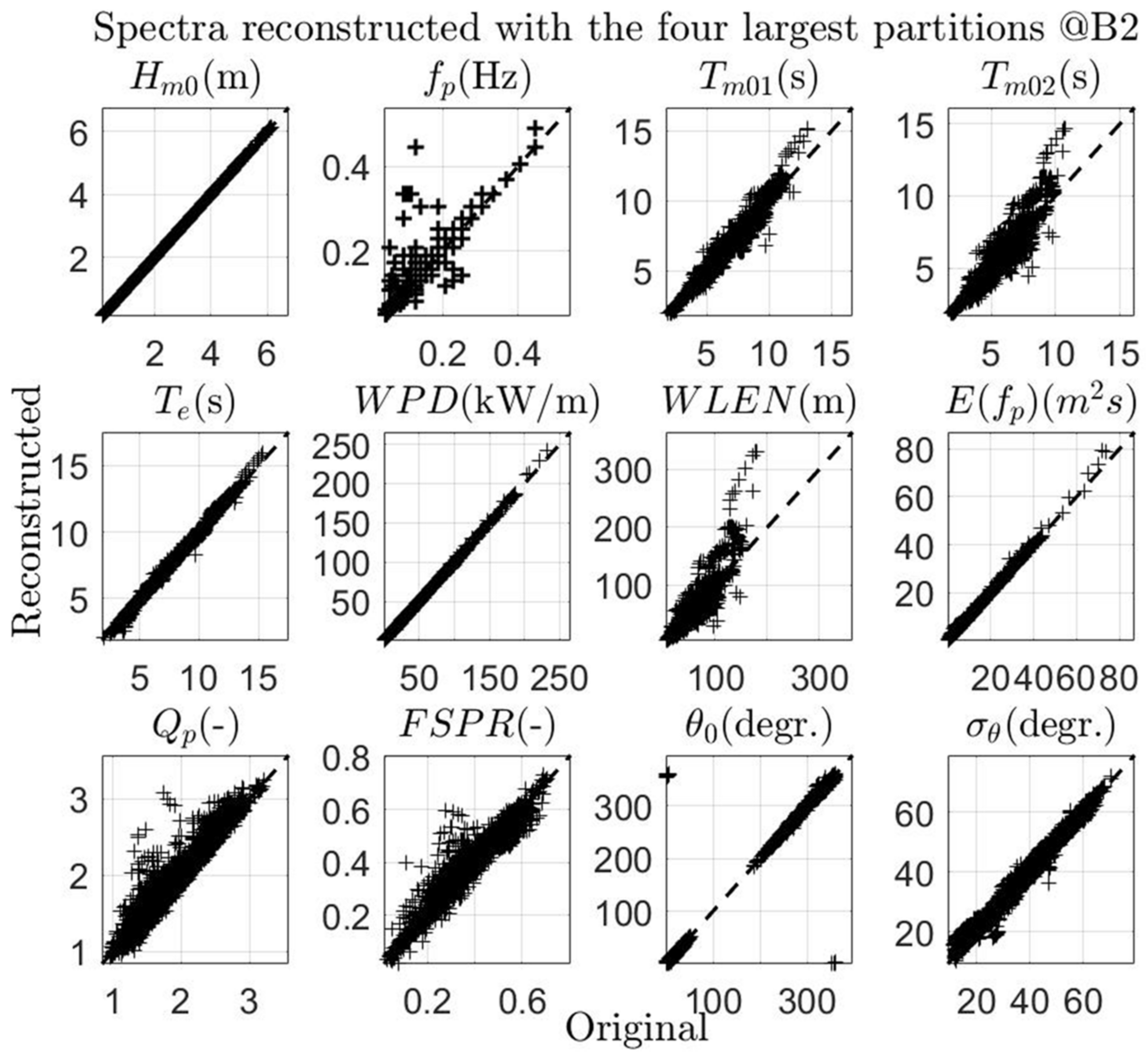
Figure 5 and Figure 6 show that with more RPs involved in the LSM fittings, better agreement with the original KPs can be obtained, except for the KP $f_p$. Specifically, with $n^{fr}=4.6$, further increment (reduction) in R (MAE) can be observed for the KPs associated with spectral bandwidth (i.e., $Q_p$ and $FSPR$,) than for the others; the opposite trends for the two KPs mentioned above can be found with $n^{tl}=4.3$. However, with higher $n^{fr}$ involved in the fitting, the critical KPs of period and wavelength present improvement in terms of both R and MAE, but the goodness of fit of those KPs is reduced much more when $n^{tl}$ is lower. Nevertheless, the KP $H_{m0}$ remains unaffected by the $n$ strategies. Considering the above results, we recommend adoption of the strategy of $n^{fr}=3$ and $n^{tl}=6$.

Another technical key point deserving further discussion is the maximum number of partitions that should be involved in Equation (18).

Table 7. Correlation coefficient (R) of the KPs derived from the original and the reconstructed spectra (with the three and six largest partitions) at check point B2. The values of R are expressed as the differences to those obtained from the original spectra and the reconstructed ones using the four largest partitions.

	KPs	${\mathit{H}}_{\mathit{m}0}$	${\mathit{f}}_{\mathit{p}}$	${\mathit{T}}_{\mathit{m}01}$	${\mathit{T}}_{\mathit{m}02}$	${\mathit{T}}_{\mathit{e}}$	$\mathit{W}\mathit{P}\mathit{D}$	$\mathit{W}\mathit{L}\mathit{E}\mathit{N}$	$\mathit{E}\left({\mathit{f}}_{\mathit{p}}\right)$	${\mathit{Q}}_{\mathit{p}}$	$\mathit{F}\mathit{S}\mathit{P}\mathit{R}$	${\mathit{\theta }}_{0,\mathit{x}}$	${\mathit{\theta }}_{0,\mathit{y}}$	${\mathit{\sigma }}_{\mathit{\theta }}$
Part.
Largest3		0	−0.008	0.000	0.000	−0.001	0.000	0.000	0.000	−0.003	−0.004	0.000	0.000	−0.002
Largest6		0	0.012	0.000	0.000	0.000	0.000	0.000	0.000	0.001	0.001	0.000	0.000	0.000

and

Table 8. Mean absolute error (MAE) of the KPs derived from the original and the reconstructed spectra (with the three and six largest partitions) at check point B2. The values of MAE are expressed as the differences to those obtained from the original spectra and the reconstructed ones using the four largest partitions.

	KPs	${\mathit{H}}_{\mathit{m}0}$  $\left(\mathbf{m}\right)$	${\mathit{f}}_{\mathit{p}}$  $\left(\mathbf{Hz}\right)$	${\mathit{T}}_{\mathit{m}01}$  $\left(\mathbf{s}\right)$	${\mathit{T}}_{\mathit{m}02}$  $\left(\mathbf{s}\right)$	${\mathit{T}}_{\mathit{e}}$  $\left(\mathbf{s}\right)$	$\mathit{W}\mathit{P}\mathit{D}$ $\left(\mathbf{k}\mathbf{W}/\mathbf{m}\right)$	$\mathit{W}\mathit{L}\mathit{E}\mathit{N}$  $\left(\mathbf{m}\right)$	$\mathit{E}\left({\mathit{f}}_{\mathit{p}}\right)$ $\left({\mathbf{m}}^2\mathbf{s}\right)$	${\mathit{Q}}_{\mathit{p}}$	$\mathit{F}\mathit{S}\mathit{P}\mathit{R}$	${\mathit{\theta }}_0$ $\left(\mathit{d}\mathit{e}\mathit{g}\mathit{r}.\right)$	${\mathit{\sigma }}_{\mathit{\theta }}$ $\left(\mathit{d}\mathit{e}\mathit{g}\mathit{r}.\right)$
Part.
Largest3		0	0.000	0.010	0.000	0.010	0.010	0.100	0.003	0.003	0.001	0.100	0.063
Largest6		0	0.000	0.000	0.000	0.000	0.000	0.000	0.000	−0.001	0.000	0.000	−0.006

illustrate the R and MAE values of the KPs at check point B2 derived from the original and the reconstructed spectra, where the latter were reconstructed with the three and six largest partitions. All the R and MAE values are expressed as the differences to those obtained from the original spectra and the reconstructed ones using the four largest partitions, as described in Section 3.

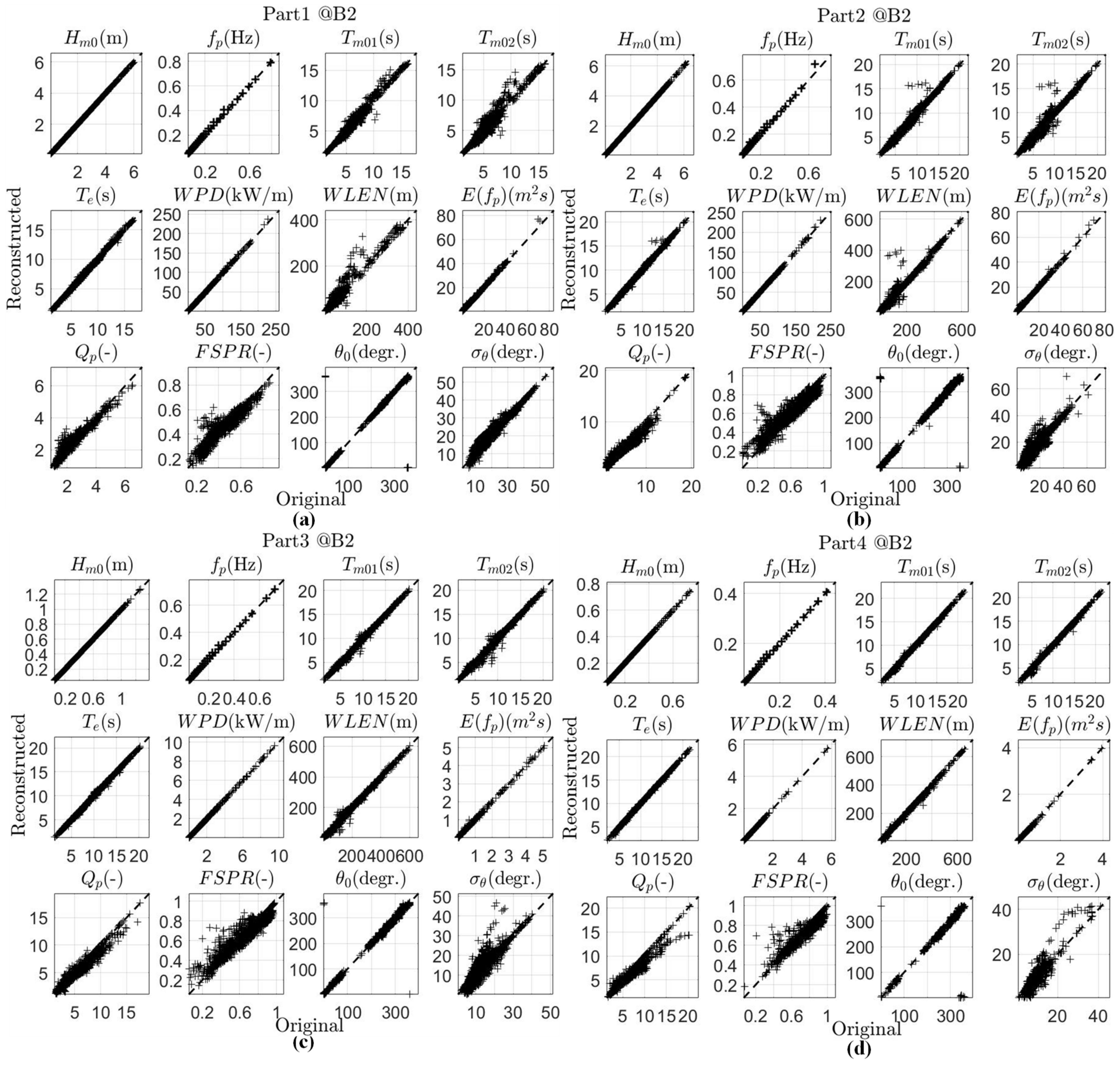
As can be seen from Table 7 and Table 8, the errors of the KPs derived from the spectra reconstructed with the three largest partitions increase slightly in comparison with those calculated based on the spectra rebuilt with the four largest partitions (as Part0 shown in Table 3 and Table 4), while the errors remain similar to those of the four largest partitions even though more partitions (the six largest) are considered. Similar results can also be observed at check points B1 (Tables S13 and S14), B3 (Tables S15 and S16), and B4 (Tables S17 and S18), the associated tables can be found in the Supplementary Material. Such findings confirm the fact that the number of coexisting wave systems (partitions) is fewer than four in most cases at point B2 (see the sampling number in Table 3 and Table 4). Therefore, the use of no more than four partitions to reconstruct a spectrum in this study is appropriate. In fact, consideration of just four significant wave systems (i.e., wind waves and the first, second, and third primary swell) can satisfy most sea states in real oceans; however, the use of fewer wave systems in the reconstruction might also be acceptable, e.g., wind waves with only one swell partition, which could further reduce the required storage space. Therefore, we recommend that the maximum number of partitions involved in the reconstruction should be based on the prevailing sea state of the nested domain.

The new approach can also be applied to observed 2D wave spectra. However, owing to the random property of ocean waves, observed spectra may comprise more noises or spurious peaks, making the identification of significant wave systems more difficult, as well as the computation of RPs more burdensome. Therefore, some noise-removal or smoothing procedures (e.g., [57]) should be performed before the spectrum preservation and reconstruction; and consequently, certain insignificant details of the spectra might be ignored.

5. Conclusions

This paper described a new approach for the preservation and reconstruction of 2D wave spectra, and the results of application of the proposed approach to boundary conditions in nested wave modeling are also presented.

Traditionally, each wave spectrum saved on the nesting boundaries could require more than 1000 storage units, in accordance with the size of the spectral space. In the newly proposed preservation approach, a certain 2D spectrum is first separated into several partitions, each of which contains only one spectral peak. By performing LSM fitting with the newly proposed GUFSM and by introducing the Maximum Entropy Method, the 1D frequency spectrum and directional distribution of each identified partition can be represented by eleven and four RPs, respectively. Consequently, given that four primary wave systems (partitions), i.e., wind waves and the first, second, and third primary swell, might coexist in each spectrum, the number of storage units occupied in preservation of a spectrum could be reduced to a maximum of $\left(11+4\right)\times 4=60$.

The corresponding proposed reconstruction approach can rebuild arbitrary 2D spectra with the preserved RPs, and the reconstructed spectra can be used as boundary conditions in nested wave modeling. To validate the agreement between the reconstructed and the original spectra, and to determine the feasibility of adopting the reconstructed spectra in nested modeling, simulations of the wave fields were conducted for the Wanning offshore area (Hainan, China). Comparisons of the original and the reconstructed spectra at the boundary points revealed that key features such as the wave height, wave period, propagation direction, and particularly wave energy flux of the original spectra could be retained intact in the reconstructed spectra. The wave fields simulated using the reconstructed boundaries conformed well with those forced by the original boundary conditions, and the spectral statistics derived from the two sets of simulated fields also presented a high level of agreement. The results of this study prove the feasibility of using the newly proposed approach in nested wave simulations.

The proposed approach allows spectral information, i.e., the RPs, of the entire simulated domain to be saved in long-term wave simulations with more acceptable storage consumption, and given that the RPs can be suitably preserved, simulations with finer spatial resolution can then be conducted free of the limitations of predefined boundaries. The above-mentioned properties of the new method could help support engineering projects concerning wave environments, research focused on wave climatology, and studies associated with wave energy assessment.