
Estimation of Urban Evapotranspiration at High Spatiotemporal Resolution and Considering Flux Footprints

State Key Laboratory of Water Resources and Hydropower Engineering Science, Wuhan University, Wuhan 430072, China
*
Author to whom correspondence should be addressed.
Remote Sens. 2023, 15(5), 1327; https://doi.org/10.3390/rs15051327
Submission received: 1 January 2023
/
Revised: 21 February 2023
/
Accepted: 23 February 2023
/
Published: 27 February 2023
(This article belongs to the Topic Hydrology and Water Resources Management)
Abstract
:Evapotranspiration (ET) estimations at high spatiotemporal resolutions in urban areas are crucial for extreme weather forecasting and water management. However, urban ET estimation remains a major challenge in current urban hydrology and regional climate research due to highly heterogeneous environments, human interference, and a lack of observations. In this study, an urban ET model, called the PT-Urban model, was proposed for half-hourly ET estimations at a 10 m resolution. The PT-Urban model was validated using observations from the Hotel Torni urban flux site during the 2018 growing season. The results showed that the PT-Urban model performed satisfactorily, with an R2 and root-mean-square error of 0.59 and 14.67 W m−2, respectively. Further analysis demonstrated that urban canopy heat storage and shading effects are essential for the half-hourly urban energy balance. Ignoring the shading effects led to a 38.7% urban ET overestimation. Modeling experiments further proved that flux footprint variations were critical for the accurate estimation of urban ET. The setting source areas either as an invariant 70% historical footprint or as a circle with a 1 km radius both resulted in poor performances. This study presents a practical method for the accurate estimation of urban ET with high spatiotemporal resolution and highlights the importance of real-time footprints in urban ET estimations.
1. Introduction
By 2050, 70% of the world’s population will live in urban areas [1]. Globally, such urbanization profoundly alters the energy balance and water cycle processes [2,3,4]. Evapotranspiration (ET) is known to link the water and energy exchanges between the Earth’s surface and the atmosphere and is sensitive to urbanization [5,6,7]. Almost all extreme hydrometeorological events, such as floods and urban heat islands (UHIs), are inseparable from ET [8,9]. Therefore, urban ET research can advance our understanding of urban climate extremes and water resource management [10,11,12]. Although analyses of urban ET are critical for understanding human living environments, studies on ET in urban areas are relatively rare compared with those in natural or agricultural regions [13,14].
The studies on urban ET are mainly limited by the highly heterogeneous underlying land surfaces and anthropogenic activities [15]. Specifically, the spatiotemporal heterogeneity of urban environments (i.e., land cover, microclimate, and energy components) hinders the application of ET models in urban areas [16]. Remote sensing-based ET estimation methods provide promising potential in urban areas. Some of the widely applied methods include the surface energy balance (SEB) model, the Penman–Monteith (PM) model, and potential ET (or reference crop ET) methods. SEB models estimate ET as the residual of the surface energy balance from satellite remote sensing images [17]. Zhang and Chen [18] compared the performances of three variants of SEB models in urban areas and found that special urban conditions limited the performance of manually selected extreme grids for calculating temperature gradients. The PM model comprehensively considers the principles of aerodynamic processes and surface energy balance, as well as concepts such as the stomatal resistance of vegetation, to estimate ET from moisture-limited surfaces [19]. Boegh et al. [20] compared the performance of the PM model in crop, forest, and urban regions and found that the model’s performance was poor in urban regions. PM models are challenging to implement because numerous parameters (e.g., aerodynamic resistance) are difficult to estimate in urban regions [20]. Potential ET methods consist of a series of ET models (e.g., the crop coefficient model [21], the Priestly-Taylor Jet Propulsion Laboratory (PT-JPL) model [22], and the Global Land Evaporation Amsterdam Model (GLEAM) [23]) that estimate the actual ET by imposing conversion coefficients on the potential ET. The conversion coefficients account for the effects of different variables on the actual ET. Studies have shown that potential ET methods perform well on various underlying surfaces [24,25,26], implying that these methods have great flexibility in complex and heterogeneous urban areas. However, the calculations of conversion coefficients in urban areas have rarely been investigated.
The energy balance of urban surfaces is more complex than that of homogeneous underlying surfaces, owing to fragmented land use types and building morphologies [27]. Currently, the eddy covariance (EC) system is the most advanced latent heat observation method in urban areas [28,29]. However, unavoidable systematic errors in EC data occur because of measurement instrument errors [30] and energy non-closure problems due to footprint mismatches [31]. In urban areas, the reliability of flux data is further exacerbated by urban morphology [32]. Usually, inaccuracies in EC data can be reduced using the Bowen ratio energy balance (BREB) method-based energy non-closure correction [33] and the same source areas for each component in the energy balance [34]. The energy non-closure correction method has been applied to flux data processing for urban ET estimations using SEB [35] and crop coefficient estimations and has achieved limited success. Grimmond and Oke [36] demonstrated that footprint-weighted flux data could improve the performance of the Penman equation in urban areas. Similarly, Vulova et al. [37] proved that the footprint-weighted normalized difference vegetation index (NDVI) could significantly improve the capability of an AI-based ET model for urban ET estimations. However, these applications ignored the mismatching source areas of different energy balance components and did not consider the footprints in the urban ET model development and parameter calibration. Furthermore, urban canopy (i.e., buildings and impervious surfaces) heat storage cannot be ignored, and it can be an important source of urban latent heat during the day [38]. The shade from buildings has a direct and large impact on the air temperatures and net radiation within shaded areas [39], resulting in a more heterogeneous urban energy balance and microclimate. Fortunately, high-frequency on-site observation and remote sensing technologies provide multi-scale observations over heterogeneous urban underlying surfaces [40,41]. This enables us to develop and validate methods for high spatiotemporal resolution urban ET estimations [9].
Therefore, the primary objective of this study was to propose a half-hourly urban ET model based on potential ET methods (i.e., the PT-Urban model) and consider the footprint and urban morphology at a 10 m resolution. In this study, data from the Hotel Torni and Fire Station urban flux sites in Helsinki, Finland, were used to demonstrate the model’s capabilities. For the PT-Urban model, the latent heat (LE) flux was corrected by the urban surface energy balance, considering the shading effect and urban canopy heat storage within the footprints. The major parameters in the PT-Urban model were calibrated using the footprint-weighted values of the simulation against the observations. The effects of shading and footprints on the ET estimation were investigated using different modeling scenarios. The specific objectives of this study were as follows: (1) to investigate the importance of urban canopy heat storage for ET estimations; (2) to establish a new method for estimating urban evapotranspiration by considering the effects of shading and footprints; (3) to quantify the effects of shading and footprints on urban evapotranspiration.
2. Data and Methods
2.1. Development of the PT-Urban Model
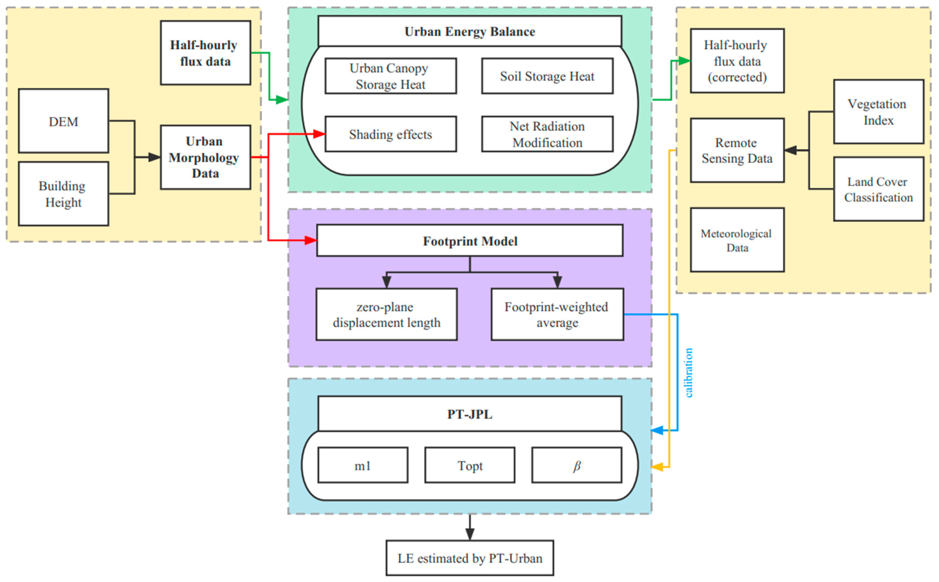
The schematic diagram in Figure 1 shows the data pathways and the main modeling modules used in this study. The proposed PT-Urban model is based on the PT-JPL model and integrates urban canopy heat, shading effects, and flux footprint modules to estimate the ET in urban environments. Building height data were used to calculate the dynamic shading of the PT-Urban model and the zero-plane displacement height of the footprint model. The net radiation and other components of the half-hourly urban energy balance were calculated according to shading maps and meteorological data. The flux data were corrected using the BREB method. All input data for the LE estimation are footprint-weighted values calculated using the footprint model. The PT-Urban model can estimate the urban ET with a spatiotemporal resolution of 10 m per half hour using remote sensing and meteorological data.
2.2. PT-JPL ET Model
Fisher et al. [22] proposed the PT-JPL model to estimate evapotranspiration by limiting potential evapotranspiration (PET) using a series of factors. In the PT-JPL model, the total LE was estimated as the sum of the following three components: vegetation canopy transpiration (), soil evaporation (), and vegetation canopy interception evaporation (). Each component of PET was calculated using available energy and then constrained to real LE by physiological plant features and soil moisture conditions. The model was driven by the following five input variables: Rn (net radiation), NDVI, EVI, Ta, and relative humidity (RH). The following equations were used to calculate the total LE:
where is the relative surface wetness, is the plant temperature constraint, is the plant moisture constraint, is the soil moisture constraint, is the PT coefficient set at 1.26, is the slope of the saturation vapor pressure to the temperature curve (KP °C−1), is the psychrometric constant (0.066 kPa °C−1), is the net radiation from the vegetation canopy interception (; W m−2), and is the net radiation received at the soil surface (W m−2). and were calculated using Equations (16) and (25). According to Beer [42] and Denmead and Millar [43], can be estimated as follows:
where is the extinction coefficient of radiation [44] and is the leaf area index. The was calculated as follows:
where and is the ratio of photosynthetically active radiation of the vegetation canopy [45]. Various eco-physiological limiting factors in the model were obtained from the following equations:
where is the optimum growth temperature of the vegetation, is the vapor pressure deficit, is the sensitivity index of to , and is the ratio of photosynthetic radiation absorbed by the vegetation canopy. The values of and are calculated as follows:
where , , , and are semi-empirical parameters.
2.3. Identification of Flux Footprint
A flux footprint is the zone of the surface upwind from an instrument that contributes to a measured vertical flux (e.g., of water vapor or carbon dioxide) between the ground and the atmosphere. The flux observed by EC systems is not from a fixed region but a footprint that varies with wind direction, wind speed, and subsurface characteristics around each site [46]. The variation of the source areas (or footprints) is often ignored for homogeneous surfaces but is not negligible for highly heterogeneous urban regions. In this study, the source areas of the vapor flux (i.e., LE) of each period were generated using the footprint model proposed by Kormann and Meixner [46].
The sizes and forms of the source areas, , can be calculated as follows:
where is the effective measurement height, is the standard deviation of the cross-stream wind component, is the wind direction, is the friction velocity, and is the Obukhov length. The half-hourly values of , , , and were obtained from observations at the Hotel Torni site.
The value of was calculated as follows:
where is the measurement height and is the zero-plane displacement height (i.e., the height at which the wind speed would become zero).
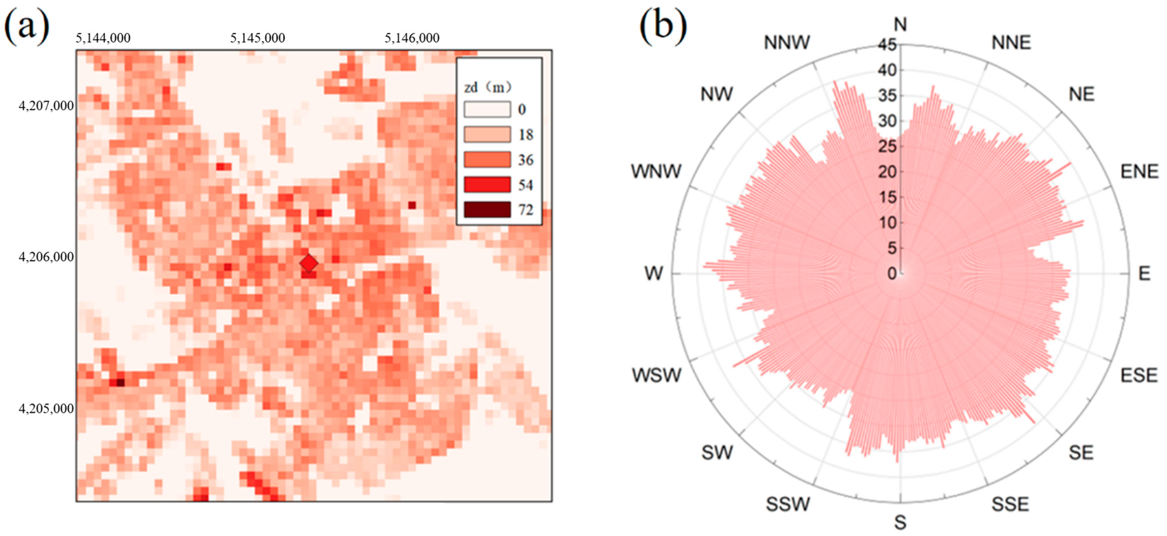
The spatial heterogeneity of the aerodynamic parameter cannot be ignored in urban areas; therefore, it cannot be an invariant value when calculating the real-time urban flux footprint. The Quantum Geographic Information System (QGIS) [47], a plugin in the Urban Multi-Scale Environmental Predictor (UMEP), was implemented to calculate gridded and windward from a digital surface model (DSM), which was calculated using the digital elevation model (DEM) and building height data from the European Environment Agency (https://land.copernicus.eu/local/urban-atlas, accessed on 22 September 2021). The for each 50 m grid area (, as shown in Figure 2a) was calculated following the method proposed by Kanda et al. [48]. For each degree, the values (, as shown in Figure 2b) were computed using the QGIS with a 1000 m radius and a 1° wind direction search interval, producing databases of for 360 wind directions.
A single value must be derived from the heterogeneous map to calculate the footprint. Once calculated, the scale and shape of the footprint determine the area. To solve this iterative problem, the initial was set as according to the wind direction. The was used to estimate the initial footprint, and the footprint was used to delimit the . The method proposed by Kljun et al. [49] was implemented to calculate the footprint-weighted from the gridded within the footprint areas. The specific calculation process is as follows (shown in Figure 3):
Step 1: The initial footprint was calculated according to the from the wind direction for each period.
Step 2: The footprint-weighted of the iteration ith () was calculated from the within the footprint.
Step 3: A footprint closer to the real footprint was calculated according to the mean in Step 2.
Steps 2 and 3 were repeated until the difference in the footprint-weighted between two adjacent iterations was less than 1 m.
2.4. Influences of Urban Morphology on Net Radiation Estimation
An accurate estimation of the spatial heterogeneity of the net radiation is essential for ET calculations [50,51]. The complexity of the net radiation calculation in urban areas arises from the highly heterogeneous urban land cover and urban morphology. Building shading can significantly influence the energy balance, especially at half-hourly time scales [52]. The net radiation is usually calculated using (16), which was proposed by Humes et al. [53] and is as follows:
where is the downward shortwave radiation (W m−2), is the downward longwave radiation (W m−2), is the upward longwave radiation, and is the surface albedo.
In urban areas, shortwave and longwave radiation vary spatiotemporally because of architectural shadings. In this study, , , and were calculated using (17), (18), and (19) following Lindberg et al. [54], Jonsson et al. [55], and Lindberg [56]. The equations are as follows:
where , , and are the direct, diffuse global solar radiation, accounts for shadow as a Boolean value (presence = 0 or absence = 1), is the altitude angle of the sun above the horizon, is the sky value factor (SVF), which represents the ratio of the sky hemisphere visible from the ground, is the incoming longwave radiation, where , and are the wall and ground emissivity, respectively, and are the surface and air temperatures, and is the Stefan–Boltzmann constant. The , , and were obtained from the Fire Station sites. The was set as 0.15. This model allows for the calculation of from the , , and RH using the approach of Reindl et al. [57]. The is calculated as follows:
2.5. Energy Closure Correction at Footprints Scale
In urban areas, the surface energy balance equation can be expressed by (22) and (23) as proposed by Oke [27], which are as follows:
where is the heat storage during the calculation period, is the urban canopy heat storage, is the soil heat storage, is the anthropogenic heat, and is the heat carried by advection. The and values can be ignored in the energy balance calculations on the half-hourly scale in this research as is much smaller than other components and the emissions of are lower in summer noon [61]. The value of was calculated using (16). The half-hourly urban canopy heat storage was calculated using the empirical equation proposed by Camuffo and Bernardi [62], which is as follows:
where is the time-varying slope of the net radiation and , , and are the linear fitting parameters. The parameters , , and are set as 0.35, 0.28 h, and −40 W m2,, respectively, according to Oke and Cleugh [38]. The three items in Equation (24) account for the real-time increment, time delay item, and offset amount of the urban canopy heat storage.
The half-hourly was calculated using the empirical equations proposed by Santanello and Friedl [63], which are as follows:
where represents the daily variations in the soil surface temperature. The parameters A and B are empirical constants and are set as 0.91 and 0.56, respectively.
The source areas of H and LE are different from the components of radiation observations because of the different measurement techniques and processes that lead to the non-closure of the energy balance [64,65]. In this study, the BREB method [33] was implemented to address the system error of the flux data observed by the EC system. The non-closure part, D, is determined by the following:
where and are the latent and sensible heat observed by the EC system between the hours of 10:00–15:00 every half hour, respectively. The Bowen ratio is more stable and representative during this period [33]. This residual caused by the system error is redistributed to latent and sensible heat according to the Bowen ratio [65]. The , and values were mapped to the same spatial resolution as the land cover data using (16), (24), and (25), respectively. The corrected LE and H values were calculated as follows [66]:
where the Bowen ratio is the average ratio of to . This process ensured that the source areas of the different terms of the urban surface energy balance were consistent. Raster maps were calculated using the footprint-weighted values for each component.
2.6. Flux Data for Model Validation
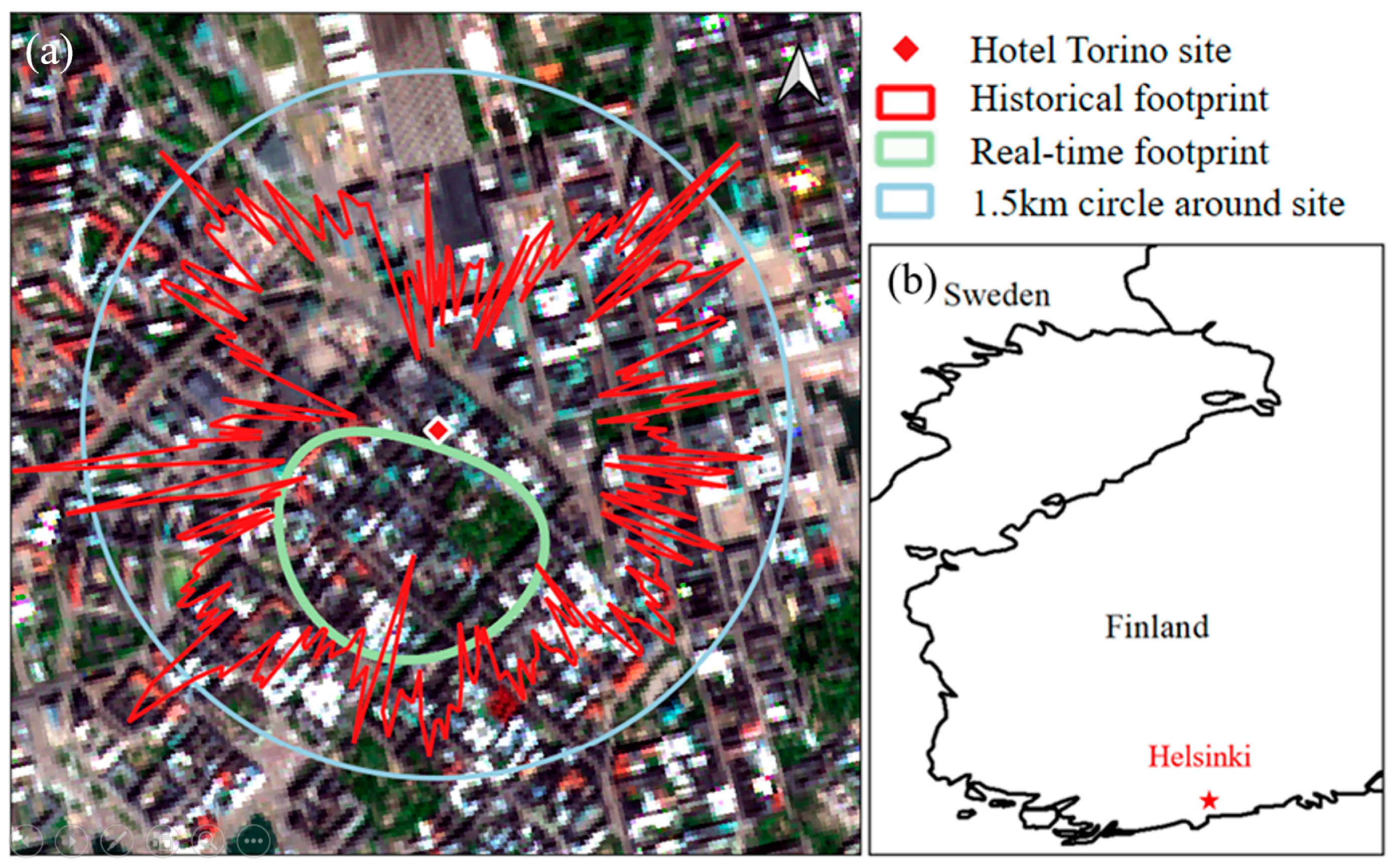
Data from two urban sites in Helsinki, the Hotel Torni flux site (60°10′04″N, 24°56′19″E) and the Fire Station site (60°12′10″N, 24°57′40″E) [67], were collected to test and validate the proposed PT-Urban model. These two sites are 400 m apart, located in the center of Helsinki, and they belong to the same urban evaporation observation project. Helsinki is on the southern coast of Finland, surrounded by the sea on three sides, and has a temperate maritime climate (Figure 4). Latent heat (LE), sensible heat (H), wind speed, humidity, and air temperature data were collected from the Hotel Torni site. Radiation data were collected from the nearby Fire Station sites. The measurements taken from May to September 2018 were used in this study.
The following half-hourly LE observations were excluded from the data set: (1) values outside the range of 0–500 W m−2 [68] (to avoid any extreme or abnormal values observed by the EC systems); (2) measurements collected during precipitation or up to 4 h after rain events (as the EC systems have poor performance on rainy days); (3) measurements without available high-quality vegetation indices; (4) measurements for which the required data for footprint estimation was missing or was insufficient to calculate the 90% footprint likelihood; (5) observations not made between the hours of 10:00 and 15:00 (as the Bowen ratio is stable during this period); (6) measurements collected during polar nights (from October–April). Following filtration, 109 half-hourly data groups were used for both the footprint estimations and the ET estimations.
2.7. High-Resolution Land Cover Data of the Study Site
The land cover classification (LCC) map used in this study was the Finer Resolution Observation and Monitoring of Global Land Cover dataset at a 10 m resolution (FROM-GLC10), which was developed by [69]. The FROM-GLC10 was derived from Sentinel-2 data in 2017 and processed using Google Earth Engine. The LCC data were found to be 73% accurate when validated against the 2015 validation sample [69]. FROM-GLC10 contains ten land use types, whereas the study area has only six, which are as follows: forest, grassland, wetland, water, impervious surface, and bare land.
The NDVI and enhanced vegetation index (EVI) were used to represent the effect of vegetation on the regional ET and calculate the leaf area index (LAI). High-resolution land cover data were clipped to the research area, as shown in Figure 4. Both NDVI and EVI were calculated from the Sentinel-2 reflected radiance (https://www.usgs.gov/centers/eros, accessed on 22 September 2021) as follows:
where , and are the spectral bands at near-infrared (842 nm), red (665 nm), and blue (490 nm) wavelengths, respectively.
Only images with less than 10% cloud cover in the region of interest that were taken within 15 days of other available data were selected. Lastly, each pixel was linearly interpolated to the daily values under the assumption that the day-to-day fluctuations of the NDVI were small within 15 days during the non-growing season. Data with high spatial resolution can reflect the refined vegetation in fragmented urban landscapes.
2.8. Model Calibration and Evaluation
The three most sensitive parameters (m1, Topt, and β) of PT-JPL, which were identified by Zhang et al. [70], were calibrated against the corrected LE values. About two-thirds of the available data (66 out of 109) were randomly selected as calibrating datasets, and the rest were used as the validation dataset.
A genetic algorithm (GA) was applied to optimize the parameters of the PT-Urban model [71]. The following three criteria were selected to assess the model’s performance: coefficient of determination (R2), root-mean-square error (RMSE), and relative bias (bias). The objective function (f) for the calibration consists of the Nash–Sutcliffe efficiency (NSE; [72]) and relative bias. The mathematical equations of the three criteria and objective function (f) for the parameter optimization are as follows:
where sim and obs are the half-hourly footprint-weighted LE and observed LE, respectively. N represents the sample size. The variables with overbars denote the average values. The RMSE can vary from 0 to +∞, while the R2 and bias can range from 0–1.0 (or 100%). The model performs best when R2 approaches 1.0 and the RMSE and bias approach zero. An R2 value of 1.0 indicates that the estimated LE shows a completely linear relationship with the observed values. An RMSE value of zero indicates that all points lie on the regression line. A bias value of zero implies that the volumes of the estimated and observed values are the same and that there is no systematic error.
3. Results
3.1. Urban Surface Energy Balance at Footprint Scale
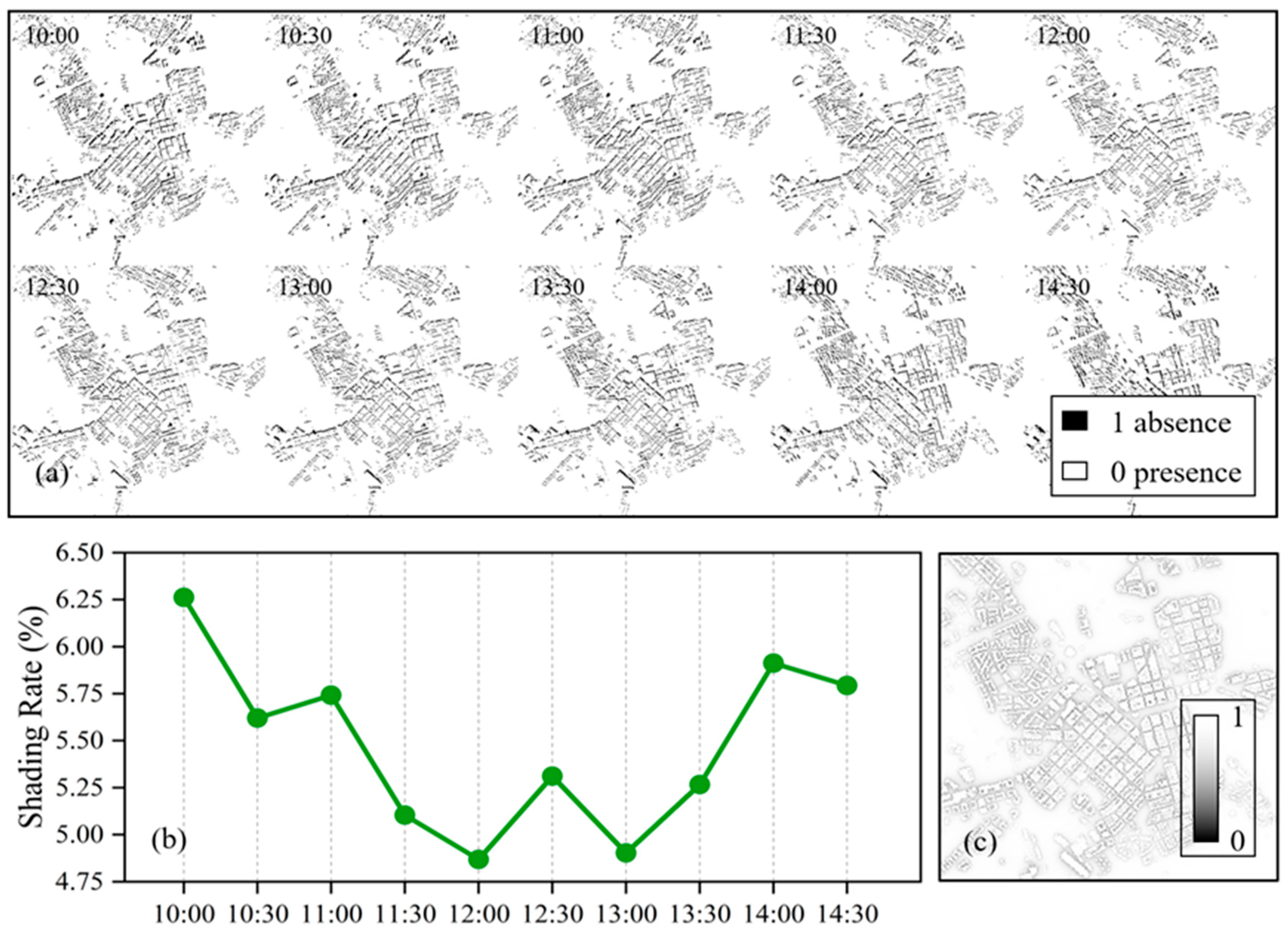
Figure 5a shows the Boolean shadow map of the study area, derived by the UMEP module at different times. The shadows moved from the northwest of the buildings to the northeast from 10 am to 3 pm. As shown in Figure 5b, the shading area ratio first decreased and then increased, with a mean value of 5.48% and maximum and minimum values of 6.26% and 4.82% at 10 am and 12 am, respectively. Figure 5c shows the sky view factor (SVF) of the study area. The closer a point is to a building and the higher the building density, the lower the SVF value at that point. The SVF varies from 0.21–1.0, with a mean value of 0.89, as shown in Figure 5c. The shaded areas and SVF values are highly heterogeneous, which could significantly influence the urban surface energy balance in different areas and at different times.
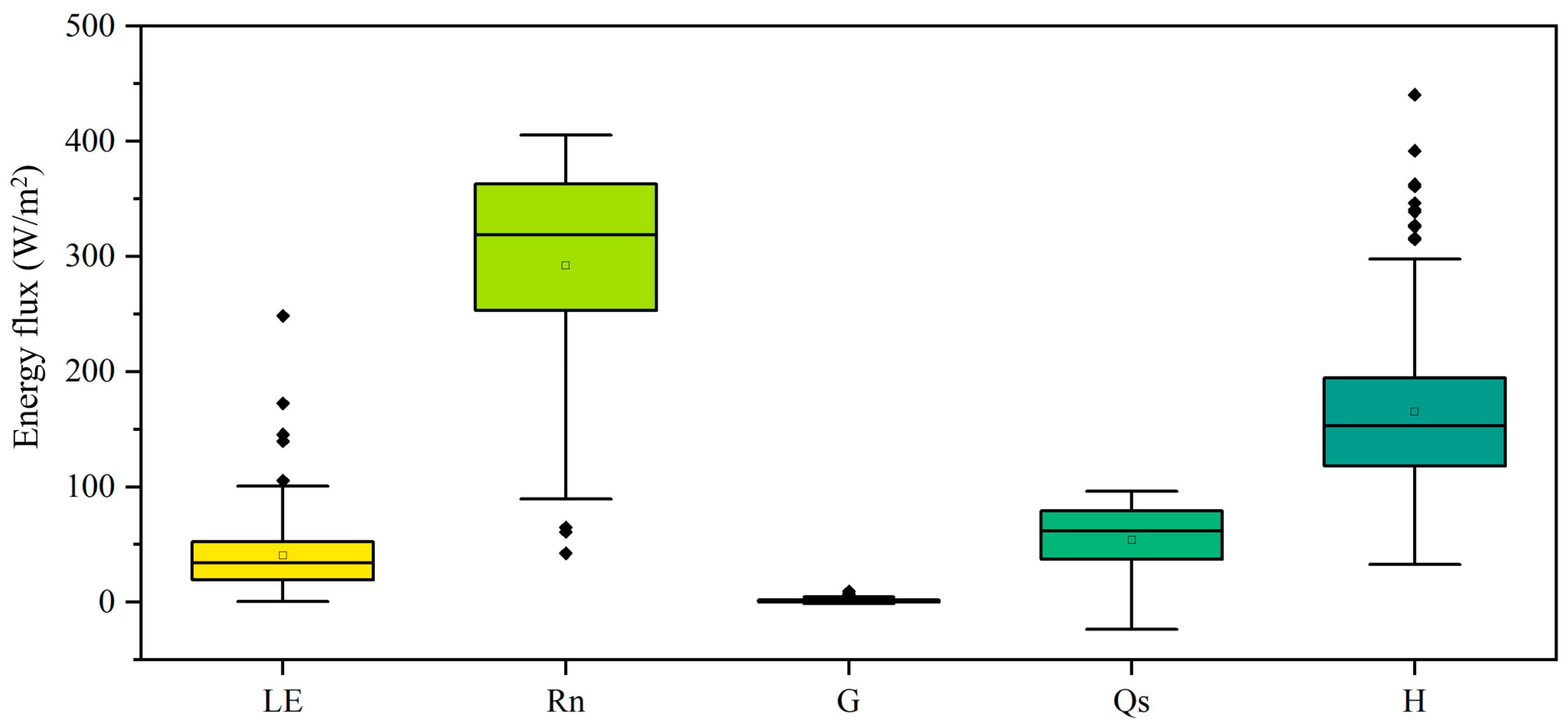
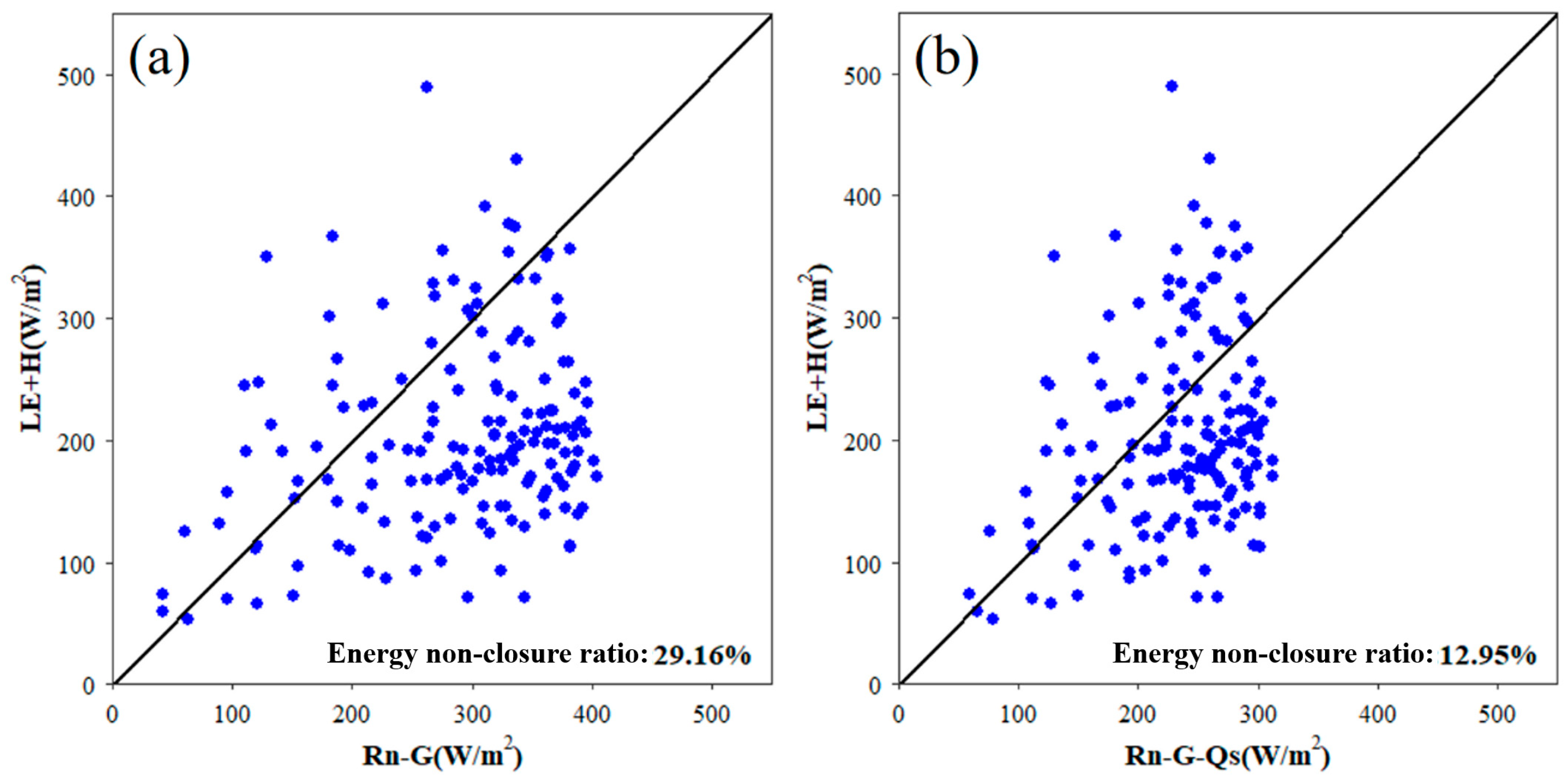
Figure 6 shows the half-hourly mean footprint-weighted Rn, G, Qs, LE, and H values for the study period. The mean values of these components are 282.11, 5.29, 54.17, 40.61, and 165.39 W m−2, respectively. The values shown in Figure 6 suggest that the footprint-weighted average urban canopy heat storage (Qs) is a non-negligible item in the energy balance equation, as it accounts for 29.7% of the available input energy. Figure 7 compares the energy balances calculated with and without considering the urban canopy heat storage (Qs). The net energy input during the study period was compared with the sum of the latent and sensible heat. The energy balance non-closure ratio was higher when the urban canopy heat storage was ignored. The consideration of the urban canopy heat can reduce the urban energy balance non-closure ratio from 29.2% to 13.0%. Therefore, urban canopy heat storage is very important for urban surface energy balance calculations, and ignoring this term would lead to significant energy closure problems.
3.2. Performance of the Proposed PT-Urban Model
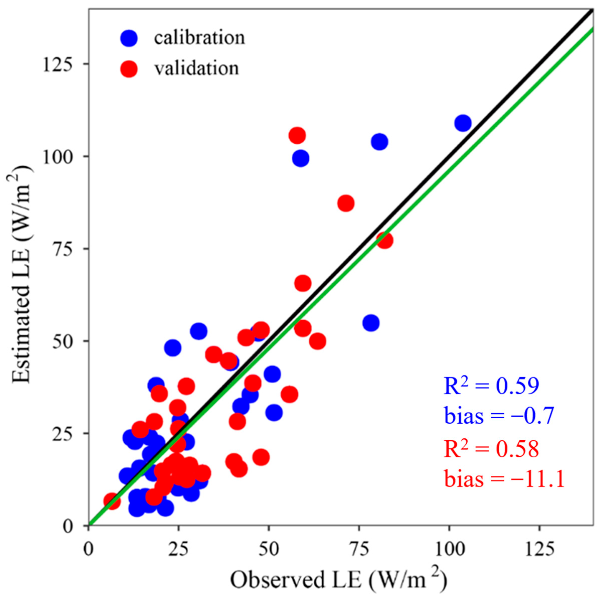
The optimal m1, Topt, and β values for the Hotel Torni site are 1.405, 18.7, and 0.55, respectively. Figure 8 compares the estimated footprint-weighted LE with the observed LE by the EC system during the calibration and validation periods. For the calibration, the estimated half-hourly LE values were highly correlated with the observed values, with an R2 value of 0.59. The fitted linear correlation line between the observed and estimated half-hourly LE values without intercept was slightly lower than 1:1, with a slope of 0.95. The RMSE and relative bias of the estimated half-hourly LE values were 14.67 W m−2 and −4.5%, respectively. During the validation, the RMSE, relative bias, and R2 were 14.70 W m−2, −11.1, and 0.58, respectively, which were close to those of the calibration. Generally, the PT-Urban model performed satisfactorily at the Hotel Torni site.
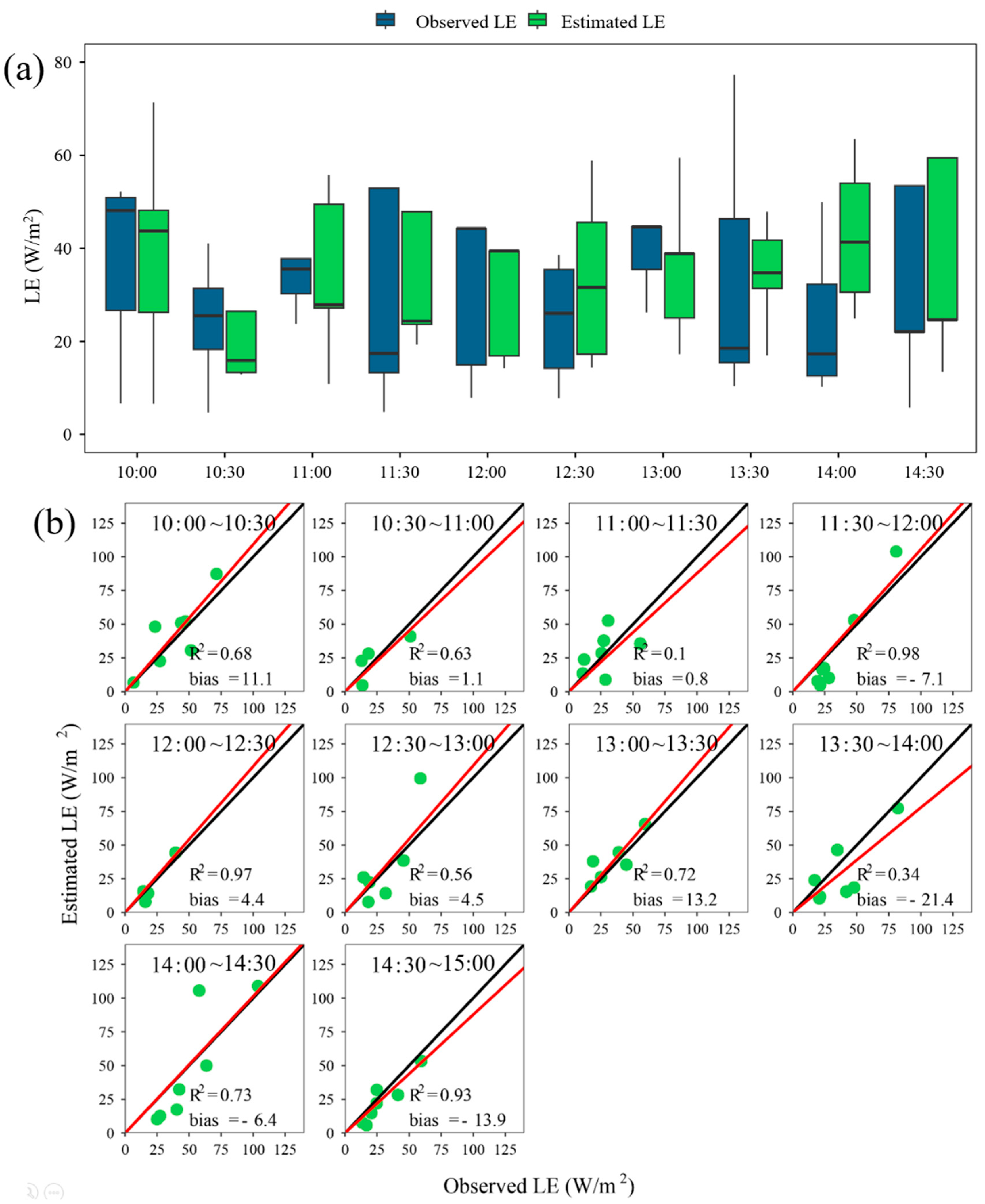
Figure 9 shows the estimated and observed LE values for each half hour during the study period. The median estimated and observed values were relatively consistent before 13:00. The inter-quantile ranges of the estimated and observed values differed at different half-hourly intervals. The R2 values for each half-hourly period varied from 0.1–0.98. The relative bias values varied from −13.9% to 13.2%.
The PT-Urban model performed better from 11:30 to 12:00, 12:00 to 12:30, and 14:30 to 15:00, during which the R2 values were over 0.9. The linear regression slopes without intercept varied from 0.83–1.18. In general, the PT-Urban model effectively captured the dynamics of the half-hourly LE observed by the flux tower.
The histogram in Figure 10 shows the three estimated components of the LE (canopy transpiration (LEc), canopy interception evaporation (LEi), and soil evaporation (LEs)) during the study period. The mean LEc, LEs, and LEi values are 20.63, 5.23, and 4.18 W m−2, respectively. The pie chart in Figure 10, which depicts the proportions of each component, shows that the LEc was the largest component of the total LE (approximately 64.9%) at the study site. LEs and LEi accounted for 20.0% and 15.1% of the total evaporation, respectively. Figure 10 indicates that the vegetation transpiration was the main source of LE at the Hotel Torni site.
3.3. Impacts of Footprints and Shadings on Urban ET Estimation
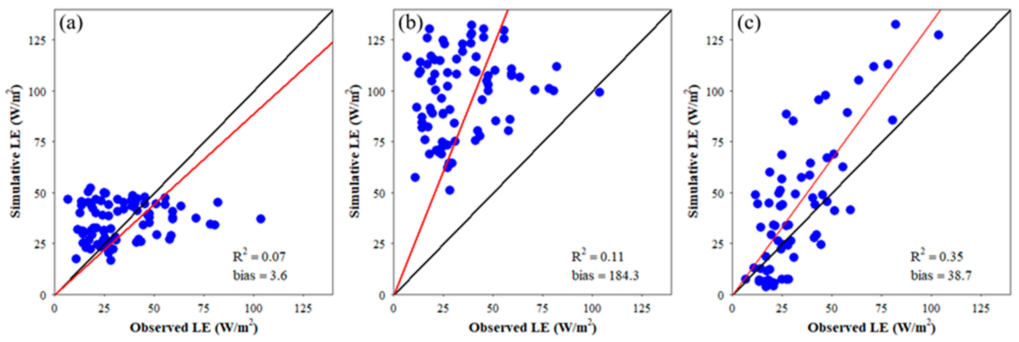
The capabilities of the PT-Urban model to estimate the urban LE with three different source areas and the influence of shading effects are compared in Table 1 and Figure 11. The three chosen source areas are as follows: a circle with a radius of 1.0 km around the site, a 70% historical footprint area, and a real-time half-hourly flux footprint (Figure 4). The LE estimated by the PT-Urban model from the different source areas is an area-weighted value. Figure 11a,b show the performance of the PT-Urban model with invariant source areas of 70% historical footprint and a circle with a 1 km radius around the site, respectively. The LE values calculated from the historical footprint average of 70% (R2 = 0.07; Figure 11a) and the 1 km radius around the site (R2 = 0.11; Figure 11b) had much lower R2 values than those estimated from the dynamic footprints (R2=0.59; Figure 8). The historical footprint average of 70% led to an LE with an RMSE of 16.25 W m−2. The LE estimated from the fixed circle was overestimated by 184.3%, with an RMSE of 70.48 W m−2. The slopes of the fitted line without intercept for the 70% historical footprint average and circle scenarios are 0.90 and 2.44, respectively. Figure 11a,b indicate that the consideration of dynamic footprints is of critical importance for the PT-Urban model when estimating high spatiotemporal resolution LE in urban regions, as shown in Figure 8.
Figure 11c shows the performance of the PT-Urban model without considering the effects of shading. Compared with the results shown in Figure 8, ignoring the impact of shading led to a significant (38.7%) overestimation of the LE. The ignorance of shading effects also led to a decrease in the R2 values from 0.59 (Figure 8) to 0.35 (Figure 11c) and an increase in the RMSE values from 14.67 (Figure 8) to 28.34 W m−2 (Figure 11c). The consideration of shading effects is, therefore, crucial for half-hourly urban LE estimations.
4. Discussion
4.1. Key Factors on Urban Surface Energy Balance
According to the energy closure and LE estimation results, the half-hourly urban energy balance estimation in the PT-Urban model provided reliable energy balance closure and partition by leveraging the urban canopy heat storage and footprint (as shown in Figure 7). The urban canopy heat storage has often been ignored in previous research on urban evapotranspiration [73]. Here, we demonstrated that ignoring the urban canopy heat storage has significant detrimental effects on the estimation of half-hourly ET in urban areas. In this study, each component of the urban surface energy balance was calculated using real-time footprints. Discrepancies in the observed areas exist when observing different variables using different instruments [46,49]. For example, soil heat fluxes do not coincide with the source areas of sensible and latent heat. This error can lead to severe non-closure problems with energy balance in urban areas. Therefore, energy non-closure in urban regions may be due to two possible reasons. First, the incompleteness of the energy balance equation components and the absence of energy inputs or outputs were not considered. Second, the highly heterogeneous underlying types reinforced the scale mismatch between the observed variables [74]. In this study, all variables in the energy balance equation were calculated using raster data and treated at the footprint source area scale, making the variables consistent in scale. Although the energy balance closure method corrected the flux data of the EC systems, this method limited the available data for model training. The short time window may limit the transferability of the PT-Urban model.
4.2. Influences of Urban Morphology on Urban LE Estimation
The consideration of architectural shading in the modeling experiments resulted in a 38.7% reduction in the estimated LE values and an improvement in the model’s performance in terms of R2, RMSE, and relative bias (as shown in Figure 8 and Figure 9). Shadows influence LE values not only via incoming radiation but also through the impact of urban morphology on urban microclimates [75]. Building heights are distributed heterogeneously in urban areas, leading to spatial variations in the shading of solar radiation. In addition, the intraday change in the sun’s altitude leads to variations in the shading over time. Shading can reduce the canopy transpiration by 40% [76] and reduce the air and urban surface temperatures [77]. The influence of urban morphology in this work was concentrated on the shading effect on net radiation. However, the thermal emissions of hardscape materials, street orientation, etc., can also impact the humidity and microclimates, such as air and surface temperatures [78,79,80]. The consideration of the urban microclimate as one of numerous influencing factors and their coupling is a complex process. Therefore, a combination of microclimate models (e.g., ENVI-met [81]) is needed for urban LE estimations in the future. It should be noted that only the noon period was investigated in this study. The shading effect could be more significant if the observations were made in shaded and unshaded areas [58,77].
Aerodynamic characteristics (e.g., zero-plane displacement) are also influenced by urban morphology, which indirectly affects dynamic footprint identifications [82]. A zero-plane displacement (zd) is defined as the height at which the mean velocity is zero, owing to large obstacles, such as buildings, in the urban region. The spatial distribution of architecture causes the zd to vary at different wind speeds and wind directions [83]. To avoid complex urban numerical modeling, the dynamic footprints were calculated iteratively with different wind directions and gridded zd values in this study.
4.3. Importance of Dynamic Footprint for Half-Hourly Urban LE Estimation
The PT-Urban model with dynamic footprints performed better than that with a fixed source area in terms of both R2 and RMSE values. This suggests that real-time footprint-weighted LE values are more suitable for resolving mismatches between the source regions of different variables. The same footprint application can be seen in previous studies that verified the urban ET model proposed by Duarte Rocha et al. [68] and Peters et al. [84]. However, the footprint model has much stricter data requirements than the traditional LE model because it requires auxiliary data observed in more rigorous situations [46]. This may reduce the applicability of the PT-Urban model proposed in this study. Moreover, the consideration of both dynamic footprints and shading effects increases the computational complexity due to footprint-weighted value processing and real-time shading map calculations.
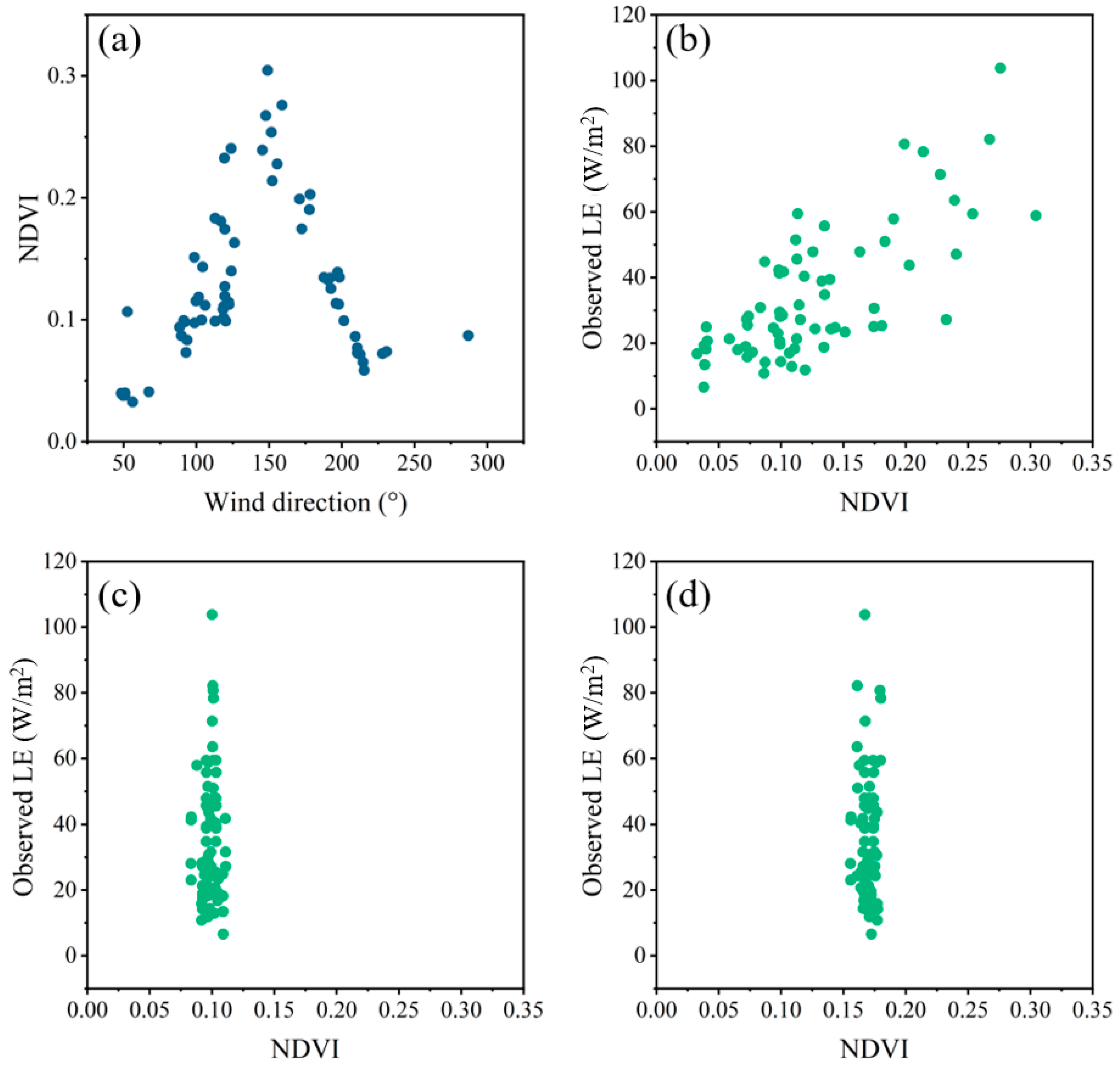
Due to the highly heterogeneous urban land cover and the high percentage of built-up areas, LE calculations largely come from vegetated areas, as shown in Figure 10. The footprint-weighted NDVI derived from dynamic footprint changes over different wind directions and the correlation between the observed LE footprint-weighted NDVI are shown in Figure 12a,b, respectively. The observed LE versus its source area-weighted NDVI derived from the two fixed source areas mentioned above is shown in Figure 12c and Figure 11d. The scatter of the historical footprint and the circle setting are near the x = 0.1 and x = 0.17 lines, as shown in Figure 12c,d, which indicates that changes in the site-based observed LE are only related to fluctuations in the climatic conditions on an hourly time scale. This is in accordance with calculations made under the assumption of homogeneous underlying surfaces [85,86] rather than heterogeneous urban land covers. Figure 12 suggests that the intraday variation in wind direction could significantly affect the observed LE and footprint-weighted NDVI. It also highlights that dynamic footprints are of critical importance for estimating half-hourly urban LE correctly. Therefore, in addition to the meteorological conditions (e.g., air temperature and net radiation), the phenological conditions of vegetation in the dynamic footprints are also necessary in urban LE modeling.
In this study, the PT-Urban model still faces a mismatch problem with the input data. This study only tried to make a more comprehensive consideration of the variables that are more important for urban ET estimations. The net radiation and air temperature were corrected to footprint scales. However, other meteorological forcing data used in this study, such as relative humidity, are still site observations and have not been corrected. The issue of mismatch is still a problem that needs further research. Furthermore, the large computational time for high spatiotemporal footprints and LE estimations limited the quantity of data for training and validating the proposed model. Although the PT-Urban model is essentially a physically process-based model rather than a data-driven model, the applicability and transferability of the proposed new method have to be further demonstrated under various conditions and with more data.
5. Conclusions
In this study, a half-hourly urban ET model, called the PT-Urban model, was proposed using flux, remote sensing, meteorological, and urban morphology data. Field observations from the Hotel Torni and Fire Station sites in Helsinki, Finland, during the growing season of 2018 were selected for calibrating and validating the model. The influences of architectural shadows and dynamic footprints were considered in the proposed PT-Urban model and quantified with different modeling scenarios. The main conclusions of this study are outlined below.
Urban canopy heat storage is critical for the calculation of half-hourly LE because it accounted for 29.7% of the available input energy during the study period. Urban canopy heat storage in the urban surface energy balance can improve the energy closure ratio by 16.2%.
The PT-Urban model performed satisfactorily during the study period. The proposed model showed R2, RMSE, and bias values of 0.59, 14.67 W m−2, and −4.5% during the study period, respectively.
The consideration of shading effects and dynamic footprints is of critical importance for urban ET estimations. Considering the shading effects can reduce ET overestimations by 38.7%, while without dynamic footprints, the estimated urban ET can be significantly biased, not only in the total quantity but also in the proportionate contributions of the three different components.
Supplementary Materials
The following supporting information can be downloaded at: https://www.mdpi.com/article/10.3390/rs15051327/s1.
Author Contributions
Conceptualization, L.Z.; methodology, L.Z.; software, L.Z.; validation, L.Z. and M.L.; formal analysis, L.Z.; investigation, L.Z.; resources, L.Z.; data curation, L.Z. and Y.M.; writing—original draft preparation, L.Z.; writing—review and editing, L.Z., S.Q., and L.C.; visualization, L.Z.; supervision, L.Z.; project administration, L.Z.; funding acquisition, L.C. All authors have read and agreed to the published version of the manuscript.
Funding
This research was funded by the National Natural Science Foundation of China (41890822), the “Western Light”-Key Laboratory Cooperative Research Cross-Team Project of the Chinese Academy of Sciences (xbzg-zdsys-202103), and the Natural Science Foundation of Hubei Province (2022CFA094).
Data Availability Statement
The data used in study are all publicly available and corresponding references and/or links are provided in the manuscript.
Acknowledgments
The authors would like to thank the Ministry of Education and Culture of Finland for providing the Hotel Torni flux site and the Fire Station site flux data, as well as the Copernicus Programme and the European Environment Agency for providing the morphology data used in this paper.
Conflicts of Interest
The authors declare no conflict of interest.
References
- Department of Economic and Social Affairs Population Division. World Urbanization Prospects: The Revision of 2018; United Nations: New York, NY, USA, 2019. [Google Scholar]
- Chen, Z.; Gong, Z.; Yang, S.; Ma, Q.; Kan, C. Impact of Extreme Weather Events on Urban Human Flow: A Perspective from Location-Based Service Data. Comput. Environ. Urban Syst. 2020, 83, 101520. [Google Scholar] [CrossRef] [PubMed]
- Liu, Y.; Wang, Z.; Sun, Q.; Erb, A.M.; Li, Z.; Schaaf, C.B.; Zhang, X.; Román, M.O.; Scott, R.L.; Zhang, Q.; et al. Evaluation of the VIIRS BRDF, Albedo and NBAR Products Suite and an Assessment of Continuity with the Long Term MODIS Record. Remote Sens. Environ. 2017, 201, 256–274. [Google Scholar] [CrossRef]
- Zhao, Q.; Li, Z.; Shah, D.; Fischer, H.; Solís, P.; Wentz, E. Understanding the Interaction between Human Activities and Physical Health under Extreme Heat Environment in Phoenix, Arizona. Health Place 2023, 79, 102691. [Google Scholar] [CrossRef] [PubMed]
- Benton, G.S.; Blackburn, R.T.; Snead, V.O. The Role of the Atmosphere in the Hydrologic Cycle. Trans. Am. Geophys. Union 1950, 31, 61. [Google Scholar] [CrossRef]
- Gentine, P.; Massmann, A.; Lintner, B.R.; Hamed Alemohammad, S.; Fu, R.; Green, J.K.; Kennedy, D.; Vilà-Guerau de Arellano, J. Land–Atmosphere Interactions in the Tropics—A Review. Hydrol. Earth Syst. Sci. 2019, 23, 4171–4197. [Google Scholar] [CrossRef] [Green Version]
- Oki, T.; Kanae, S.; Musiake, K. Global Hydrological Cycle and World Water Resources. Science 2003, 28, 206–214. [Google Scholar] [CrossRef] [Green Version]
- Li, X.; Li, Y.; Chen, A.; Gao, M.; Slette, I.J.; Piao, S. The Impact of the 2009/2010 Drought on Vegetation Growth and Terrestrial Carbon Balance in Southwest China. Agric. For. Meteorol. 2019, 269–270, 239–248. [Google Scholar] [CrossRef]
- Wang, Y.; Zhang, Y.; Ding, N.; Qin, K.; Yang, X. Simulating the Impact of Urban Surface Evapotranspiration on the Urban Heat Island Effect Using the Modified RS-PM Model: A Case Study of Xuzhou, China. Remote Sens. 2020, 12, 578. [Google Scholar] [CrossRef] [Green Version]
- Litvak, E.; McCarthy, H.R.; Pataki, D.E. A Method for Estimating Transpiration of Irrigated Urban Trees in California. Landsc. Urban Plan. 2017, 158, 48–61. [Google Scholar] [CrossRef] [Green Version]
- Noori, B.; Nouri, H. Estimation of Urban Evapotranspiration through Vegetation Indices Using WorldView2 Satellite Remote Sensing Images. In Proceedings of the International Conference on Sustainable Development, Strategies and Challenges with a Focus on Agriculture, Natural Resources, Environment and Tourism, Tabriz, Iran, 25 February 2015. [Google Scholar]
- Nouri, H.; Stokvis, B.; Galindo, A.; Blatchford, M.; Hoekstra, A.Y. Water Scarcity Alleviation through Water Footprint Reduction in Agriculture: The Effect of Soil Mulching and Drip Irrigation. Sci. Total Environ. 2019, 653, 241–252. [Google Scholar] [CrossRef]
- Nouri, H.; Beecham, S.; Kazemi, F.; Hassanli, A.M. A Review of ET Measurement Techniques for Estimating the Water Requirements of Urban Landscape Vegetation. Urban Water J. 2013, 10, 247–259. [Google Scholar] [CrossRef]
- Saher, R.; Stephen, H.; Ahmad, S. Urban Evapotranspiration of Green Spaces in Arid Regions through Two Established Approaches: A Review of Key Drivers, Advancements, Limitations, and Potential Opportunities. Urban Water J. 2021, 18, 115–127. [Google Scholar] [CrossRef]
- Arnfield, A.J. Two Decades of Urban Climate Research: A Review of Turbulence, Exchanges of Energy and Water, and the Urban Heat Island. Int. J. Climatol. 2003, 23, 1–26. [Google Scholar] [CrossRef]
- Pataki, D.E.; McCarthy, H.R.; Litvak, E.; Pincetl, S. Transpiration of Urban Forests in the Los Angeles Metropolitan Area. Ecol. Appl. 2011, 21, 661–677. [Google Scholar] [CrossRef] [PubMed] [Green Version]
- Bastiaanssen, W.G.M.; Menenti, M.; Feddes, R.A.; Holtslag, A.A.M. A Remote Sensing Surface Energy Balance Algorithm for Land (SEBAL). 1. Formulation. J. Hydrol. 1998, 212–213, 198–212. [Google Scholar] [CrossRef]
- Zhang, T.; Chen, Y. Application of Different Remote Sensing Evapotranspiration Estimate Models in Urban Agglomeration Areas. In Proceedings of the American Geophysical Union, Fall Meeting, Washington, DC, USA, 10–14 December 2018; p. H33I-2204. [Google Scholar]
- Monteith, J.I.L. Evaporation and Environment. Symp. Soc. Exp. Biol. 1965, 19, 205–234. [Google Scholar]
- Boegh, E.; Poulsen, R.N.; Butts, M.; Abrahamsen, P.; Dellwik, E.; Hansen, S.; Hasager, C.B.; Ibrom, A.; Loerup, J.-K.; Pilegaard, K.; et al. Remote Sensing Based Evapotranspiration and Runoff Modeling of Agricultural, Forest and Urban Flux Sites in Denmark: From Field to Macro-Scale. J. Hydrol. 2009, 377, 300–316. [Google Scholar] [CrossRef]
- Allen, R.G.; Pereira, L.S.; Raes, D.; Smith, M. Crop Evapotranspiration-Guidelines for Computing Crop Water Requirements-FAO Irrigation and Drainage Paper 56. Fao Rome 1998, 300, D05109. [Google Scholar]
- Fisher, J.B.; Tu, K.P.; Baldocchi, D.D. Global Estimates of the Land–Atmosphere Water Flux Based on Monthly AVHRR and ISLSCP-II Data, Validated at 16 FLUXNET Sites. Remote Sens. Environ. 2008, 112, 901–919. [Google Scholar] [CrossRef]
- Martens, B.; Miralles, D.G.; Lievens, H.; van der Schalie, R.; de Jeu, R.A.M.; Fernández-Prieto, D.; Beck, H.E.; Dorigo, W.A.; Verhoest, N.E.C. GLEAM v3: Satellite-Based Land Evaporation and Root-Zone Soil Moisture. Geosci. Model Dev. 2017, 10, 1903–1925. [Google Scholar] [CrossRef] [Green Version]
- Luo, Z.; Guo, M.; Bai, P.; Li, J. Different Vegetation Information Inputs Significantly Affect the Evapotranspiration Simulations of the PT-JPL Model. Remote Sens. 2022, 14, 2573. [Google Scholar] [CrossRef]
- Shao, R.; Zhang, B.; Su, T.; Biao, L.; Cheng, L.; Xue, Y.; Yang, W. Estimating the Increase in Regional Evaporative Water Consumption as a Result of Vegetation Restoration Over the Loess Plateau, China. J. Geophys. Res.-Atmos. 2019, 124, 11783–11802. [Google Scholar] [CrossRef]
- Cheng, S.; Cheng, L.; Qin, S.; Zhang, L.; Liu, P.; Liu, L.; Xu, Z.; Wang, Q. Improved Understanding of How Catchment Properties Control Hydrological Partitioning Through Machine Learning. Water Resour. Res. 2022, 58, e2021WR031412. [Google Scholar] [CrossRef]
- Oke, T.R. The Urban Energy Balance. Prog. Phys. Geogr. Earth Environ. 1988, 12, 471–508. [Google Scholar] [CrossRef]
- Baldocchi, D.; Falge, E.; Gu, L.; Olson, R.; Hollinger, D.; Running, S.; Anthoni, P.; Bernhofer, C.; Davis, K.; Evans, R.; et al. FLUXNET: A New Tool to Study the Temporal and Spatial Variability of Ecosystem–Scale Carbon Dioxide, Water Vapor, and Energy Flux Densities. Bull. Am. Meteorol. Soc. 2001, 82, 2415–2434. [Google Scholar] [CrossRef]
- Cheng, S.; Cheng, L.; Liu, P.; Qin, S.; Zhang, L.; Xu, C.-Y.; Xiong, L.; Liu, L.; Xia, J. An Analytical Baseflow Coefficient Curve for Depicting the Spatial Variability of Mean Annual Catchment Baseflow. Water Resour. Res. 2021, 57, e2020WR029529. [Google Scholar] [CrossRef]
- Leuning, R.; van Gorsel, E.; Massman, W.J.; Isaac, P.R. Reflections on the Surface Energy Imbalance Problem. Agric. For. Meteorol. 2012, 156, 65–74. [Google Scholar] [CrossRef]
- Foken, T. The Energy Balance Closure Problem: An Overview. Ecol. Appl. 2008, 18, 1351–1367. [Google Scholar] [CrossRef]
- Lipson, M.; Grimmond, S.; Best, M.; Chow, W.T.L.; Christen, A.; Chrysoulakis, N.; Coutts, A.; Crawford, B.; Earl, S.; Evans, J.; et al. Harmonized Gap-Filled Datasets from 20 Urban Flux Tower Sites. Earth Syst. Sci. Data 2022, 14, 5157–5178. [Google Scholar] [CrossRef]
- Twine, T.E.; Kustas, W.P.; Norman, J.M.; Cook, D.R.; Houser, P.R.; Meyers, T.P.; Prueger, J.H.; Starks, P.J.; Wesely, M.L. Correcting Eddy-Covariance Flux Underestimates over a Grassland. Agric. For. Meteorol. 2000, 103, 279–300. [Google Scholar] [CrossRef] [Green Version]
- Schmid, H. Experimental Design for Flux Measurements: Matching Scales of Observations and Fluxes. Agric. For. Meteorol. 1997, 87, 179–200. [Google Scholar] [CrossRef]
- Chen, H.; Huang, J.J.; Dash, S.S.; Lan, Z.; Gao, J.; McBean, E.; Singh, V.P. Development of a Three-Source Remote Sensing Model for Estimation of Urban Evapotranspiration. Adv. Water Resour. 2022, 161, 104126. [Google Scholar] [CrossRef]
- Grimmond, C.S.B.; Oke, T.R. An Evapotranspiration-Interception Model for Urban Areas. Water Resour. Res. 1991, 27, 1739–1755. [Google Scholar] [CrossRef]
- Vulova, S.; Meier, F.; Rocha, A.D.; Quanz, J.; Nouri, H.; Kleinschmit, B. Modeling Urban Evapotranspiration Using Remote Sensing, Flux Footprints, and Artificial Intelligence. Sci. Total Environ. 2021, 786, 147293. [Google Scholar] [CrossRef] [PubMed]
- Oke, T.R.; Cleugh, H.A. Urban Heat Storage Derived as Energy Balance Residuals. Bound.-Layer Meteorol. 1987, 39, 233–245. [Google Scholar] [CrossRef]
- Ruffieux, D.; Wolfe, D.E.; Russell, C. The Effect of Building Shadows on the Vertical Temperature Structure of the Lower Atmosphere in Downtown Denver. J. Appl. Meteorol. Climatol. 1990, 29, 1221–1231. [Google Scholar] [CrossRef]
- Liu, Y.; Qiu, G.; Zhang, H.; Yang, Y.; Zhang, Y.; Wang, Q.; Zhao, W.; Jia, L.; Ji, X.; Xiong, Y.; et al. Shifting from Homogeneous to Heterogeneous Surfaces in Estimating Terrestrial Evapotranspiration: Review and Perspectives. Sci. China Earth Sci. 2022, 65, 197–214. [Google Scholar] [CrossRef]
- Zhang, Y.; Cheng, L.; Zhang, L.; Qin, S.; Liu, L.; Liu, P.; Liu, Y. Does Non-Stationarity Induced by Multiyear Drought Invalidate the Paired-Catchment Method? Hydrol. Earth Syst. Sci. 2022, 26, 6379–6397. [Google Scholar] [CrossRef]
- Beer, A. Bestimmung der Absorption des rothen Lichts in farbigen Flüssigkeiten. Ann. Phys. Chem. 1852, 162, 78–88. [Google Scholar] [CrossRef] [Green Version]
- Denmead, O.T.; Millar, B.D. Field Studies of the Conductance of Wheat Leaves and Transpiration. Agron. J. 1976, 68, 307–311. [Google Scholar] [CrossRef]
- Impens, I.; Lemeur, R. Extinction of Net Radiation in Different Crop Canopies. Arch. Für Meteorol. Geophys. Bioklimatol. Ser. B 1969, 17, 403–412. [Google Scholar] [CrossRef]
- Ross, J. Radiative Transfer in Plant Communities. Veg. Atmos. 1975, 1, 13–55. [Google Scholar]
- Kormann, R.; Meixner, F.X. An Analytical Footprint Model For Non-Neutral Stratification. Bound.-Layer Meteorol. 2001, 99, 207–224. [Google Scholar] [CrossRef]
- Lindberg, F.; Grimmond, C.S.B.; Gabey, A.; Huang, B.; Kent, C.W.; Sun, T.; Theeuwes, N.E.; Järvi, L.; Ward, H.C.; Capel-Timms, I.; et al. Urban Multi-Scale Environmental Predictor (UMEP): An Integrated Tool for City-Based Climate Services. Environ. Model. Softw. 2018, 99, 70–87. [Google Scholar] [CrossRef]
- Kanda, M.; Inagaki, A.; Miyamoto, T.; Gryschka, M.; Raasch, S. A New Aerodynamic Parametrization for Real Urban Surfaces. Bound.-Layer Meteorol. 2013, 148, 357–377. [Google Scholar] [CrossRef]
- Kljun, N.; Calanca, P.; Rotach, M.W.; Schmid, H.P. A Simple Two-Dimensional Parameterisation for Flux Footprint Prediction (FFP). Geosci. Model Dev. 2015, 8, 3695–3713. [Google Scholar] [CrossRef] [Green Version]
- Chen, X.; Su, Z.; Ma, Y.; Yang, K.; Wang, B. Estimation of Surface Energy Fluxes under Complex Terrain of Mt. Qomolangma over the Tibetan Plateau. Hydrol. Earth Syst. Sci. 2013, 17, 1607–1618. [Google Scholar] [CrossRef] [Green Version]
- Running, S.W.; Coughlan, J.C. A General Model of Forest Ecosystem Processes for regional applications I. Hydrologic Balance, Canopy Gas Exchange and Primary Production Processes. Ecol. Model. 1988, 42, 125–154. [Google Scholar] [CrossRef]
- Sakakibara, Y. A Numerical Study of the Effect of Urban Geometry upon the Surface Energy Budget. Atmos. Environ. 1996, 30, 487–496. [Google Scholar] [CrossRef]
- Humes, K.S.; Kustas, W.P.; Moran, M.S.; Nichols, W.D.; Weltz, M.A. Variability of Emissivity and Surface Temperature over a Sparsely Vegetated Surface. Water Resour. Res. 1994, 30, 1299–1310. [Google Scholar] [CrossRef]
- Lindberg, F.; Jonsson, P.; Honjo, T.; Wästberg, D. Solar Energy on Building Envelopes—3D Modelling in a 2D Environment. Sol. Energy 2015, 115, 369–378. [Google Scholar] [CrossRef]
- Jonsson, P.; Eliasson, I.; Holmer, B.; Grimmond, C.S.B. Longwave Incoming Radiation in the Tropics: Results from Field Work in Three African Cities. Theor. Appl. Climatol. 2006, 85, 185–201. [Google Scholar] [CrossRef]
- Lindberg, F.; Holmer, B.; Thorsson, S. SOLWEIG 1.0—Modelling Spatial Variations of 3D Radiant Fluxes and Mean Radiant Temperature in Complex Urban Settings. Int. J. Biometeorol. 2008, 52, 697–713. [Google Scholar] [CrossRef] [PubMed]
- Reindl, D.T.; Beckman, W.A.; Duffie, J.A. Diffuse Fraction Correlations. Sol. Energy 1990, 45, 1–7. [Google Scholar] [CrossRef]
- Bogren, J.; Gustavsson, T.; Karlsson, M.; Postgård, U. The Impact of Screening on Road Surface Temperature. Meteorol. Appl. 2000, 7, 97–104. [Google Scholar] [CrossRef]
- Gan, R.; Zhang, Y.; Shi, H.; Yang, Y.; Eamus, D.; Cheng, L.; Chiew, F.H.S.; Yu, Q. Use of Satellite Leaf Area Index Estimating Evapotranspiration and Gross Assimilation for Australian Ecosystems: Coupled Estimates of ET and GPP. Ecohydrology 2018, 11, e1974. [Google Scholar] [CrossRef]
- Dorman, M.; Erell, E.; Vulkan, A.; Kloog, I. Shadow: R Package for Geometric Shadow Calculations in an Urban Environment. R J. 2019, 11, 287. [Google Scholar] [CrossRef] [Green Version]
- Spronken-Smith, R.; Oke, T.; Lowry, W. Advection and the Surface Energy Balance across an Irrigated Urban Park. Int. J. Climatol. 2000, 20, 1033–1047. [Google Scholar] [CrossRef]
- Camuffo, D.; Bernardi, A. An Observational Study of Heat Fluxes and Their Relationships with Net Radiation. Bound.-Layer Meteorol. 1982, 23, 359–368. [Google Scholar] [CrossRef]
- Santanello, J.A.; Friedl, M.A. Diurnal Covariation in Soil Heat Flux and Net Radiation. J. Appl. Meteorol. 2003, 42, 851–862. [Google Scholar] [CrossRef]
- Aubinet, M.; Vesala, T.; Papale, D. Eddy Covariance: A Practical Guide to Measurement and Data Analysis; Springer Science & Business Media: Berlin, Germany, 2012; ISBN 978-94-007-2350-4. [Google Scholar]
- Dabberdt, W.F.; Lenschow, D.H.; Horst, T.W.; Zimmerman, P.R.; Oncley, S.P.; Delany, A.C. Atmosphere-Surface Exchange Measurements. Science 1993, 260, 1472–1481. [Google Scholar] [CrossRef] [PubMed]
- Qin, S.; Li, S.; Cheng, L.; Zhang, L.; Qiu, R.; Liu, P.; Xi, H. Partitioning Evapotranspiration in Partially Mulched Interplanted Croplands by Improving the Shuttleworth-Wallace Model. Agric. Water Manag. 2023, 276, 108040. [Google Scholar] [CrossRef]
- Järvi, L.; Hannuniemi, H.; Hussein, T.; Junninen, H.; Aalto, P.; Keronen, P.; Kulmala, M.; Keronen, P.; Hillamo, R.; Mäkelä, T.; et al. The urban Measurement Station SMEAR III: Continuous Monitoring of Air Pollution and Surface-Atmosphere Interactions in Helsinki, Finland. Boreal Environ. Res. 2009, 14 (Suppl. A), 86–109. [Google Scholar]
- Duarte Rocha, A.; Vulova, S.; van der Tol, C.; Förster, M.; Kleinschmit, B. Modelling Hourly Evapotranspiration in Urban Environments with SCOPE Using Open Remote Sensing and Meteorological Data. Hydrol. Earth Syst. Sci. 2022, 26, 1111–1129. [Google Scholar] [CrossRef]
- Gong, P.; Liu, H.; Zhang, M.; Li, C.; Wang, J.; Huang, H.; Clinton, N.; Ji, L.; Li, W.; Bai, Y.; et al. Stable Classification with Limited Sample: Transferring a 30-m Resolution Sample set Collected in 2015 to Mapping 10-m Resolution Global Land Cover in 2017. Sci. Bull. 2019, 64, 370–373. [Google Scholar] [CrossRef] [PubMed] [Green Version]
- Zhang, K.; Ma, J.; Gaofeng, Z.; Ma, T.; Han, T.; Feng, L. Parameter Sensitivity Analysis and Optimization for a Satellite-Based Evapotranspiration Model across Multiple Sites Using MODIS and Flux Data. J. Geophys. Res. Atmospheres 2016, 122, 230–245. [Google Scholar] [CrossRef]
- Grefenstette, J. Optimization of Control Parameters for Genetic Algorithms. IEEE Trans. Syst. Man Cybern. 1986, 16, 122–128. [Google Scholar] [CrossRef]
- Nash, J.E.; Sutcliffe, J.V. River Flow Forecasting through Conceptual Models part I—A Discussion of Principles. J. Hydrol. 1970, 10, 282–290. [Google Scholar] [CrossRef]
- Rwasoka, D.T.; Gumindoga, W.; Gwenzi, J. Estimation of Actual Evapotranspiration Using the Surface Energy Balance System (SEBS) Algorithm in the Upper Manyame Catchment in Zimbabwe. Phys. Chem. Earth Parts ABC 2011, 36, 736–746. [Google Scholar] [CrossRef]
- Kleissl, J.; Hong, S.-H.; Hendrickx, J.M. New Mexico Scintillometer Network: Supporting Remote Sensing and Hydrologic and Meteorological Models. Bull. Am. Meteorol. Soc. 2009, 90, 207–218. [Google Scholar] [CrossRef]
- Yu, B.; Liu, H.; Wu, J.; Lin, W.-M. Investigating Impacts of Urban Morphology on Spatio-Temporal Variations of Solar Radiation with Airborne LIDAR Data and a Solar Flux Model: A Case Study of Downtown Houston. Int. J. Remote Sens. 2009, 30, 4359–4385. [Google Scholar] [CrossRef]
- Lai, A.; Maing, M.; Ng, E. Observational Studies of Mean Radiant Temperature across Different Outdoor Spaces under Shaded Conditions in Densely Built Environment. Build. Environ. 2017, 114, 397–409. [Google Scholar] [CrossRef]
- Litvak, E.; Bijoor, N.S.; Pataki, D.E. Adding Trees to Irrigated Turfgrass Lawns May Be a Water-Saving Measure in Semi-Arid Environments. Ecohydrology 2013, 7, 1314–1330. [Google Scholar] [CrossRef]
- Ali-Toudert, F.; Mayer, H. Numerical Study on the Effects of Aspect Ratio and Orientation of an Urban Street Canyon on Outdoor Thermal Comfort in Hot and Dry Climate. Build. Environ. 2006, 41, 94–108. [Google Scholar] [CrossRef]
- Qiu, G.; Tan, S.; Wang, Y.; Yu, X.; Yan, C. Characteristics of Evapotranspiration of Urban Lawns in a Sub-Tropical Megacity and Its Measurement by the ‘Three Temperature Model + Infrared Remote Sensing’ Method. Remote Sens. 2017, 9, 502. [Google Scholar] [CrossRef] [Green Version]
- Shashua-Bar, L.; Hoffman, M.E. The Green CTTC Model for Predicting the Air Temperature in Small Urban Wooded Sites. Build. Environ. 2002, 37, 1279–1288. [Google Scholar] [CrossRef]
- Gusson, C.S.; Duarte, D.H.S. Effects of Built Density and Urban Morphology on Urban Microclimate—Calibration of the Model ENVI-Met V4 for the Subtropical Sao Paulo, Brazil. Procedia Eng. 2016, 169, 2–10. [Google Scholar] [CrossRef]
- Grimmond, C.S.B.; Oke, T.R. Aerodynamic Properties of Urban Areas Derived, from Analysis of Surface Form. J. Appl. Meteorol. Climatol. 1999, 38, 1262–1292. [Google Scholar] [CrossRef]
- Kent, C.W.; Grimmond, S.; Barlow, J.; Gatey, D.; Kotthaus, S.; Lindberg, F.; Halios, C.H. Evaluation of Urban Local-Scale Aerodynamic Parameters: Implications for the Vertical Profile of Wind Speed and for Source Areas. Bound.-Layer Meteorol. 2017, 164, 183–213. [Google Scholar] [CrossRef] [PubMed] [Green Version]
- Peters, E.B.; Hiller, R.V.; McFadden, J.P. Seasonal Contributions of Vegetation Types to Suburban Evapotranspiration. J. Geophys. Res. Biogeosciences 2011, 116. [Google Scholar] [CrossRef]
- Martens, B.; Waegeman, W.; Dorigo, W.A.; Verhoest, N.E.C.; Miralles, D.G. Terrestrial Evaporation Response to Modes of Climate Variability. Clim. Atmos. Sci. 2018, 1, 43. [Google Scholar] [CrossRef] [Green Version]
- Vergara, J.; de la Fuente, A. Intraday evaporation and heat fluxes variation at air-water interface of extremely shallow lakes in Chilean Andean Plateau. In Proceedings of the EGU General Assembly Conference, Vienna, Austria, 17–22 April 2016. EPSC2016-8300. [Google Scholar]
Figure 1.
Flowchart showing the modeling framework of the proposed PT-Urban method.

Figure 2.
(a) The 50 m × 50 m zero-plane displacement (zd) of the study area was calculated to (b) the zd in different wind directions for each degree by UMEP.
Figure 2.
(a) The 50 m × 50 m zero-plane displacement (zd) of the study area was calculated to (b) the zd in different wind directions for each degree by UMEP.

Figure 3.
Flowchart showing the calculation process of .

Figure 4.
Maps showing (a) an S2 L2A bottom-of-atmospheric true color RGB image of the Hotel Torino site with three different source areas and (b) the location of the study flux site. The 90% footprint likelihood source area of observations was at 10:00 on 24 July 2018, and the historical footprint source area was derived from the maximum 70% footprint likelihood during the study period.

Figure 5.
Plots showing (a) the Boolean shadow of the study areas at different times; (b) the variation of the shading rate in the study area; (c) the sky view factor of the study area from 10:00 to 15:00 on 24 July 2018.
Figure 5.
Plots showing (a) the Boolean shadow of the study areas at different times; (b) the variation of the shading rate in the study area; (c) the sky view factor of the study area from 10:00 to 15:00 on 24 July 2018.

Figure 6.
Boxplots showing the footprint-weighted values of each urban energy balance component at the scale of the footprint during the study period. The hollow and solid dots represent the average and abnormal values of the variables, respectively.
Figure 6.
Boxplots showing the footprint-weighted values of each urban energy balance component at the scale of the footprint during the study period. The hollow and solid dots represent the average and abnormal values of the variables, respectively.

Figure 7.
The sums of the observed latent and sensible heat by the EC system are compared with the net energy input ((a) ignoring the urban canopy storage; (b) considering the urban canopy storage heat).
Figure 7.
The sums of the observed latent and sensible heat by the EC system are compared with the net energy input ((a) ignoring the urban canopy storage; (b) considering the urban canopy storage heat).

Figure 8.
Comparison of the observed and simulated half-hourly LE values of all 109 study periods. The red and blue filled dots represent the values from the calibration and validation sets. The black and green lines are the 1:1 and linear regressed lines without intercept, respectively.
Figure 8.
Comparison of the observed and simulated half-hourly LE values of all 109 study periods. The red and blue filled dots represent the values from the calibration and validation sets. The black and green lines are the 1:1 and linear regressed lines without intercept, respectively.

Figure 9.
Boxplots showing (a) the observed (green fill) and estimated (blue fill) half-hourly LE from 10:00 to 14:30 during the study period; (b) the comparison of simulated and observed half-hourly LE. The black and red lines are the 1:1 and linear regressed lines without intercept, respectively.
Figure 9.
Boxplots showing (a) the observed (green fill) and estimated (blue fill) half-hourly LE from 10:00 to 14:30 during the study period; (b) the comparison of simulated and observed half-hourly LE. The black and red lines are the 1:1 and linear regressed lines without intercept, respectively.

Figure 10.
Histogram showing the half-hourly estimated canopy interception evaporation (LEi), soil evaporation (LEi), and canopy transpiration (LEc) during the study period. The inserted pie chart shows the proportions of each component in the total LE during the study period.
Figure 10.
Histogram showing the half-hourly estimated canopy interception evaporation (LEi), soil evaporation (LEi), and canopy transpiration (LEc) during the study period. The inserted pie chart shows the proportions of each component in the total LE during the study period.

Figure 11.
Scatter plots of the observed LE versus the estimated LE (a) from the 70% historical footprint average, (b) from a 1.0 km radius circle, and (c) without considering the shading effects.
Figure 11.
Scatter plots of the observed LE versus the estimated LE (a) from the 70% historical footprint average, (b) from a 1.0 km radius circle, and (c) without considering the shading effects.

Figure 12.
Scatter plots of (a) dynamic footprint-weighted NDVI versus wind direction; observed LE versus weighted NDVI within (b) dynamic footprints, (c) the historical footprint, and (d) the fixed circle area.
Figure 12.
Scatter plots of (a) dynamic footprint-weighted NDVI versus wind direction; observed LE versus weighted NDVI within (b) dynamic footprints, (c) the historical footprint, and (d) the fixed circle area.


Table 1.
Model performance for each scenario according to the metrics RMSE, R2, and relative bias for the PT-Urban model.
Table 1.
Model performance for each scenario according to the metrics RMSE, R2, and relative bias for the PT-Urban model.
| Sample | Shading | Source Area | RMSE (W m−2) | R2 | Bias (%) |
|---|---|---|---|---|---|
| total | yes | dynamic footprint | 14.67 | 0.59 | −4.5 |
| calibration | yes | dynamic footprint | 14.65 | 0.59 | −0.7 |
| validation | yes | dynamic footprint | 14.70 | 0.58 | −11.1 |
| total | yes | historical footprint | 16.25 | 0.07 | 3.6 |
| total | yes | 1.5 km circle area | 70.48 | 0.11 | 184.3 |
| total | no | dynamic footprint | 28.34 | 0.35 | 38.7 |
Disclaimer/Publisher’s Note: The statements, opinions and data contained in all publications are solely those of the individual author(s) and contributor(s) and not of MDPI and/or the editor(s). MDPI and/or the editor(s) disclaim responsibility for any injury to people or property resulting from any ideas, methods, instructions or products referred to in the content. |
© 2023 by the authors. Licensee MDPI, Basel, Switzerland. This article is an open access article distributed under the terms and conditions of the Creative Commons Attribution (CC BY) license (https://creativecommons.org/licenses/by/4.0/).
Share and Cite
MDPI and ACS Style
Zhou, L.; Cheng, L.; Qin, S.; Mai, Y.; Lu, M. Estimation of Urban Evapotranspiration at High Spatiotemporal Resolution and Considering Flux Footprints. Remote Sens. 2023, 15, 1327. https://doi.org/10.3390/rs15051327
AMA Style
Zhou L, Cheng L, Qin S, Mai Y, Lu M. Estimation of Urban Evapotranspiration at High Spatiotemporal Resolution and Considering Flux Footprints. Remote Sensing. 2023; 15(5):1327. https://doi.org/10.3390/rs15051327
Chicago/Turabian StyleZhou, Lihao, Lei Cheng, Shujing Qin, Yiyi Mai, and Mingshen Lu. 2023. "Estimation of Urban Evapotranspiration at High Spatiotemporal Resolution and Considering Flux Footprints" Remote Sensing 15, no. 5: 1327. https://doi.org/10.3390/rs15051327
Note that from the first issue of 2016, this journal uses article numbers instead of page numbers. See further details here.