Multi-Modal Multi-Stage Underwater Side-Scan Sonar Target Recognition Based on Synthetic Images

Abstract

Due to the small sample size of underwater acoustic data and the strong noise interference caused by seabed reverberation, recognizing underwater targets in Side-Scan Sonar (SSS) images is challenging. Using a transfer-learning-based recognition method to train the backbone network on a large optical dataset (ImageNet) and fine-tuning the head network with a small SSS image dataset can improve the classification of sonar images. However, optical and sonar images have different statistical characteristics, directly affecting transfer-learning-based target recognition. In order to improve the accuracy of underwater sonar image classification, a style transformation method between optical and SSS images is proposed in this study. In the proposed method, objects with the SSS style were synthesized through content image feature extraction and image style transfer to reduce the variability of different data sources. A staged optimization strategy using multi-modal data effectively captures the anti-noise features of sonar images, providing a new learning method for transfer learning. The results of the classification experiment showed that the approach is more stable when using synthetic data and other multi-modal datasets, with an overall accuracy of 100%.

1. Introduction

The ocean covers a vast volume and contains abundant resources. With the depletion of land resources, the development of the world economy and technology, and the continuous enhancement of military strength, countries worldwide have shifted their research focus to the ocean. Imaging Radar and Sonar (RS) are indispensable sensor devices in underwater remote sensing and can provide rich visual information about the observed area. Consequently, considerable research has been conducted on automatic target recognition [1] in sonar images. Side-Scan Sonar (SSS) emits short sound pulses, and the sound waves propagate outward in the form of spherical waves.

The sound waves are scattered when they hit objects, and the backscattered waves will be received by the transducer according to the original propagation route and converted into a series of electrical pulses. The received data of each emission cycle are arranged vertically to form a row of an SSS image, and multiple such rows are concatenated to form a complete SSS image. Due to the complexity of underwater environments and severe seabed reverberation, sonar images are affected by various types of noise, such as Gaussian, impulse, and speckle noise [2,3,4,5,6]. Noise can result in the loss of image detail, reduced contrast, and blurred edges, making SSS target identification more difficult. Therefore, target identification in sonar images acquired in harsh environments is an ongoing research challenge.

In recent years, RS target detection and recognition using Deep Learning (DL) have been extensively investigated due to the advantages of high accuracy, strong robustness, and amenity to parallelized implementations [7,8,9]. This has resulted in a new trend of using DL methods for the automated recognition of targets in SSS images. Related studies have shown that utilizing a CNN for SSS object recognition is more effective than traditional methods (K-nearest neighbors [10], SVM [11], Markov random field [12]) [13,14,15,16,17,18]. In order to extract deeper target features, Simonyan, Krizhevsky Alex, and HeKaiming et al. proposed the VGG [19], AlexNet [20], ResNet [21], and DenseNet [22] algorithms, respectively, based on Convolutional Neural Networks (CNNs). Especially in the cases of ResNet and DenseNet, the number of deep network layers is expanded to 152 and 161 layers, respectively (ResNet-152, DenseNet-161) [23,24], proving that deep network models are excellent for image recognition. However, for SSS image target recognition, where it is difficult to obtain training samples, it is challenging to develop practical DL methods.

Deep networks are generally divided into a backbone and a head. The backbone network utilizes a CNN for feature extraction [20,25,26], and the head network uses the features obtained from the backbone network to predict the target category. In target recognition using Transfer Learning (TL) methods, the backbone network is pre-trained on an external large-scale classification dataset (such as ImageNet [27]), and then, the head network is fine-tuned on the target dataset to alleviate the problem of insufficient target sample data. Pre-training on ImageNet has an advantage in general object recognition and is helpful for object recognition on small-scale datasets, such as those available for SSS [28].

Therefore, using TL methods to identify SSS targets is a practical approach and a research focus to solve the problem of SSS data shortage. Researchers have thus conducted a series of related studies on TL-based object recognition in SSS images.

2. Related Work

Regarding current research on TL, Ye, X. et al.applied VGG-11 and ResNet-18 to target recognition in SSS images under water and adopted the TL method to fine-tune the fully connected layer to address the problem of the low recognition rates caused by insufficient data samples. However, the data difference between the source and transfer datasets was not fully considered during the data transfer process, so the effect was not significantly improved [13]. Yulin, T. et al. applied TL to the target detection method. In the head network, two loss functions, the position and target recognition errors, were employed to perform position detection concurrently with target recognition. The algorithm is an improvement of YOLO [29] and R-CNN [30], but in the target detection process, the size of the feature anchor box is predetermined based on experience, limiting the detection ability of targets with large-scale changes [31,32,33]. Chandrashekar et al. utilized TL from optical to SSS images to enhance underwater sediment images and increase their signal-to-noise ratio [34]. Guanying H. et al. used semi-synthetic data and different modal data to fine-tune the parameters of VGG-19 to improve its generalization further. Using semi-synthetic data requires the target’s segmentation in the optical image, which is then transplanted into the SSS image. Only the background of the synthesized image possesses the SSS image’s characteristics, while the target does not. There is still a difference between the synthesized image and the SSS image sample, which directly affects the target recognition result [14,35].

Although TL has helped generic DL object recognition models achieve accuracies as high as 87% [13] and 97.76% [14] on small-scale SSS datasets, little attention has been paid to the following challenges:

Challenge 1: Because optical and SSS images have apparent differences in terms of perspective, noise, background noise, and resolution, current attempts to transfer optical image training models to SSS images cannot strictly meet the requirements of TL-based target recognition.

Challenge 2: For SSS images, generic DL network frameworks (such as VGG, ResNet, and others) have many parameters, making them susceptible to overfitting when trained on small sample datasets for object identification. This severely limits their generalization capability.

To tackle the first challenge, the proposed approach in this paper changes the style of the optical images using suitable transformations. Hence, the transformed image has the characteristics of noise, background noise, and resolution similar to SSS images. This reduces the discrepancies between the optical and SSS images, decreasing the occurrence of negative transfer in TL and the hindering effect of optical images on SSS images during network parameter learning, and improves the adaptability of transfer networks to SSS images.

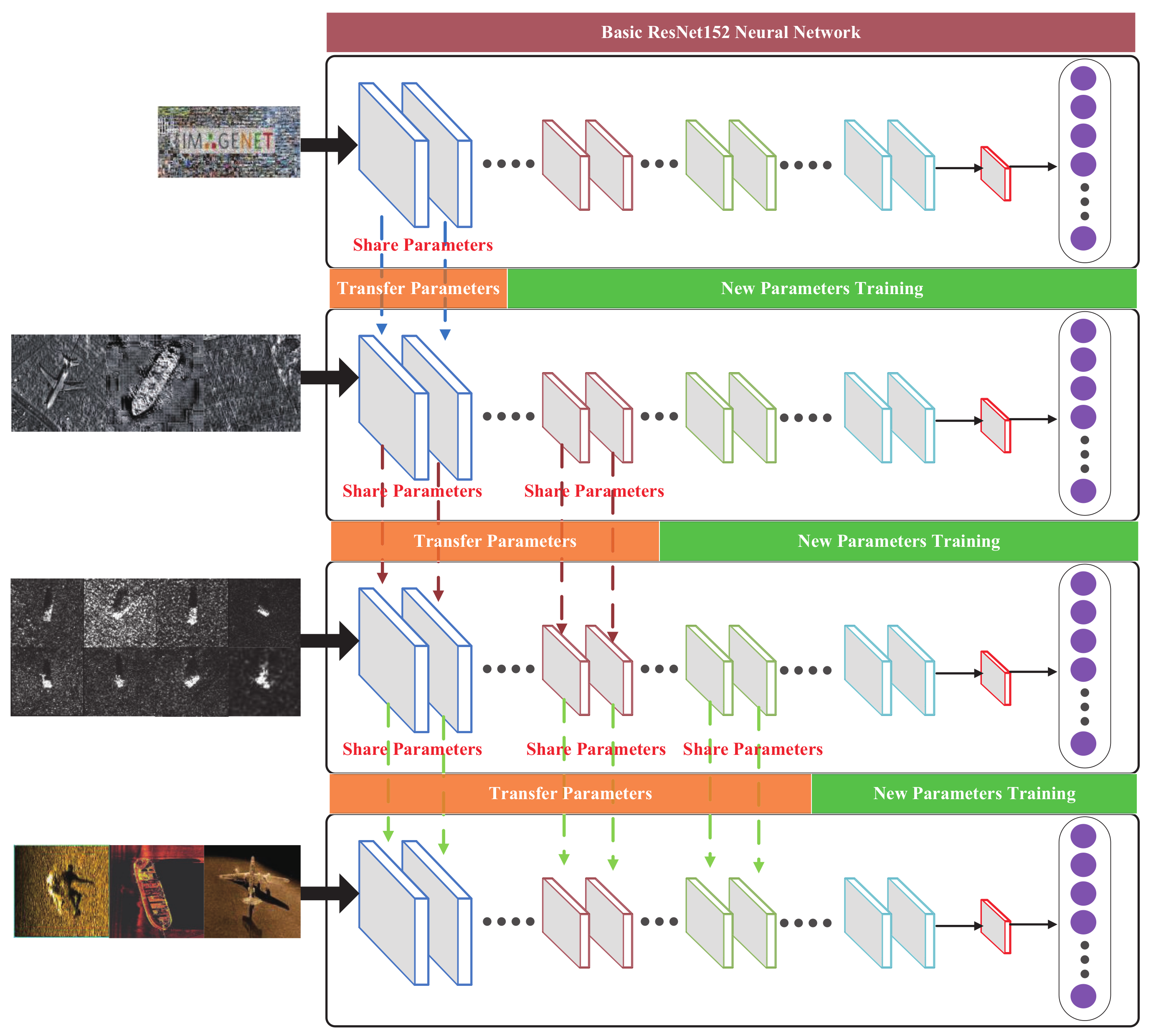
For the second challenge, it is necessary to design a particular dataset and TL strategy to pre-train a backbone network with many parameters and fine-tune the features of a head network with a smaller number of parameters based on the SSS dataset. Following a traditional TL approach, the backbone network is divided into multiple sub-backbone networks, and optical, synthetic, and SAR datasets are used in sequence to train the backbone network. In this manner, the ability of the backbone network to extract features is increased.

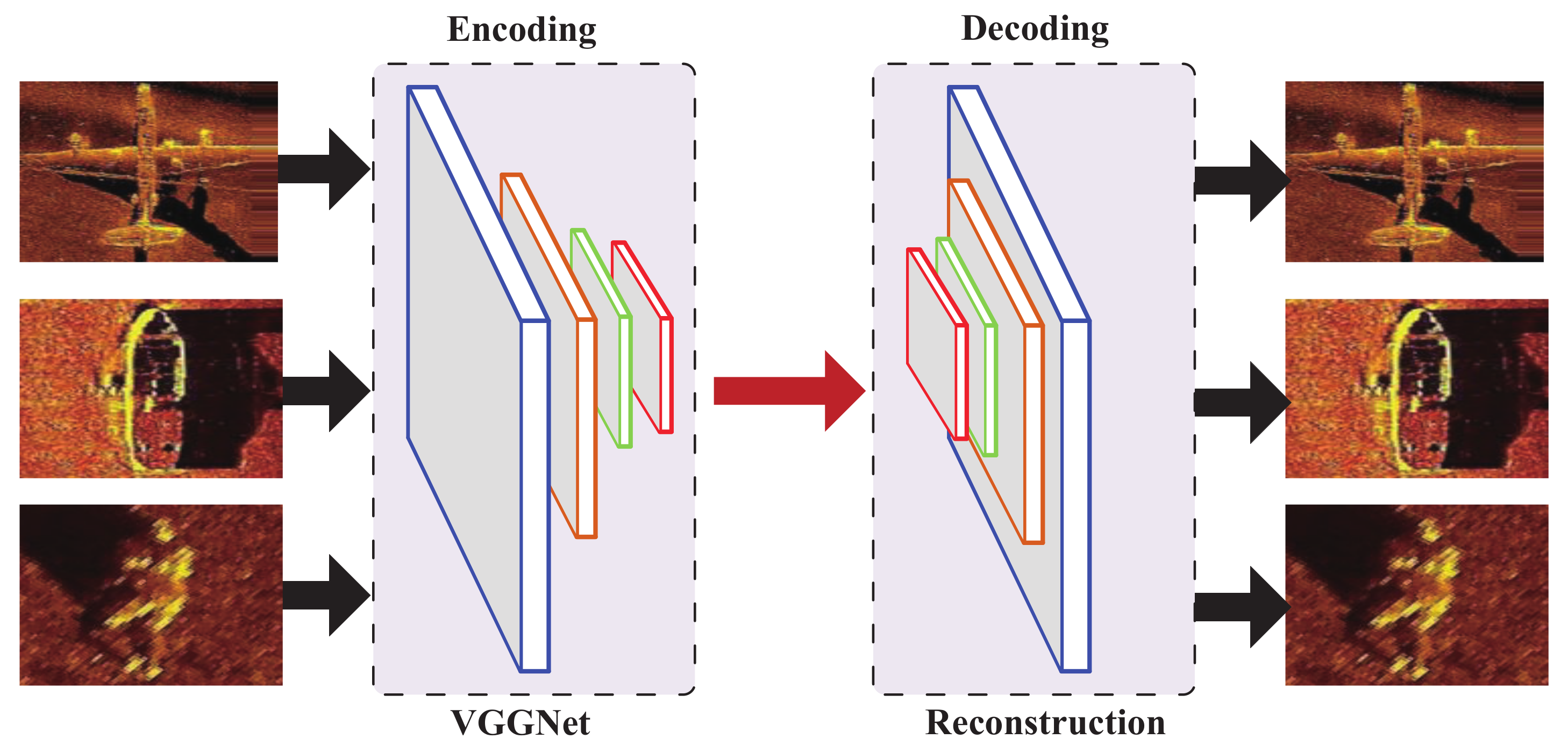
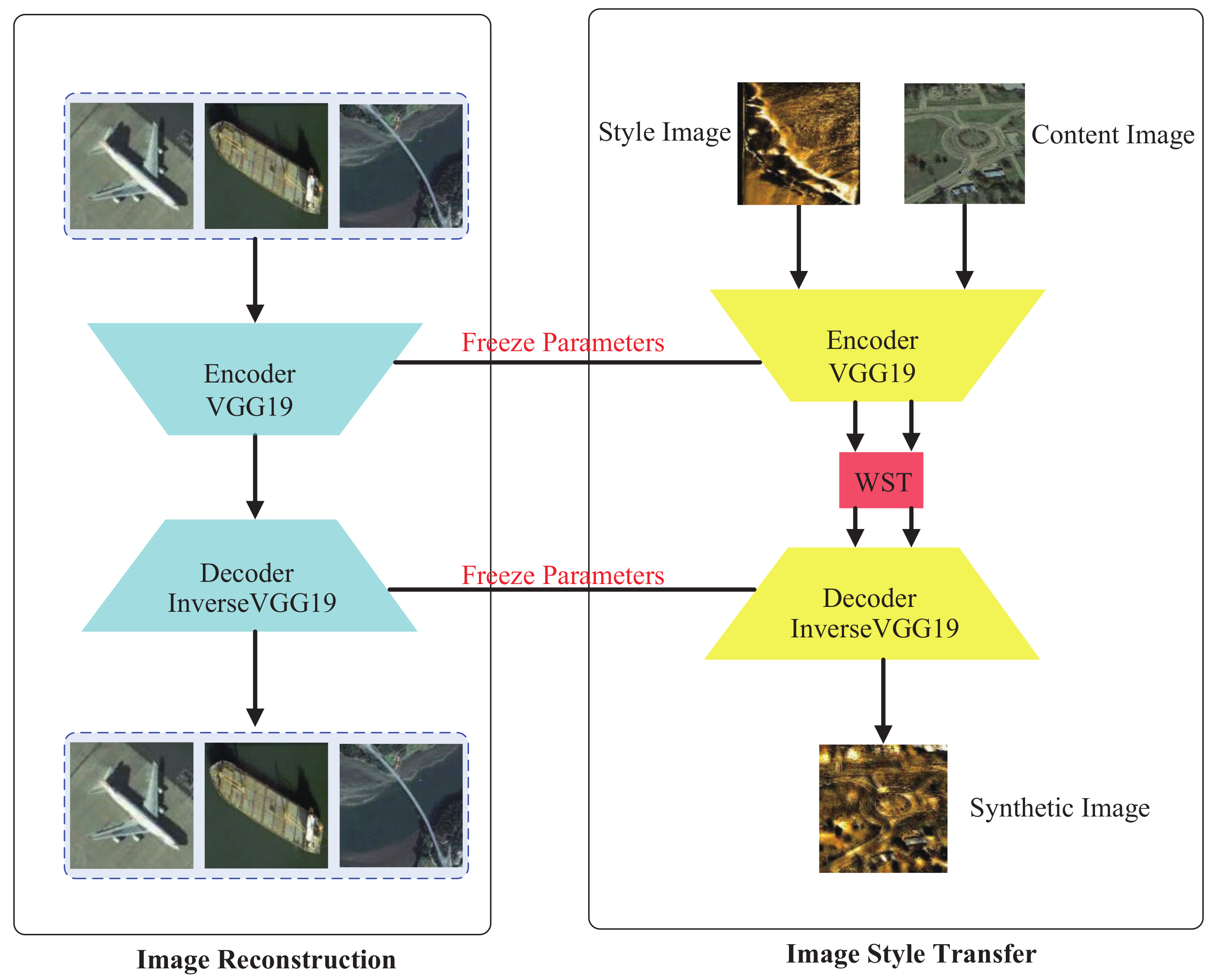
In this work, the problem of the recognition accuracy degradation caused by the difference between optical images and SSS images was addressed via TL. First, optical images were transformed through whitening and style transforms (WSTs) using an encoding–decoding model, resulting in a synthetic dataset. Then, using optical, synthetic, SAR, and SSS data, the different feature layers of the network were trained in stages to obtain stable features that were robust to interference. Finally, the features were applied to identify the SSS targets.

The main contributions of this article are summarized as follows:

1. Using the WST method, the optical target image is styled through an encoder–decoder model to achieve a simulated SSS target image with similar background noise and characteristics to the actual SSS image.

2. Based on a TL framework, a multi-modal staged parameter optimization strategy is designed. Four modal datasets (ImageNet, a transformed SSS-style, a synthetic aperture radar, and actual SSS datasets) were used, and the parameters were roughly adjusted for the backbone network’s front, middle, and rear sections and then fine-tuned. This solves the problem of network overfitting and poor generalization performance in target recognition.

3. In this paper, an image synthesis method is proposed that uses feature transformation to directly match the content and style information in the style image and combines feature transformation with a pre-trained encoder–decoder model to achieve image style conversion through simple forward transfer. This addresses the challenging problems of the simulation of targets with varying complex shapes and reduces the computational load and the effect of the too-ideal intensity distribution in the SSS image synthesis method.

The rest of this article is organized as follows: In Section 3, the image synthesis method based on an encoder–decoder model is discussed from a theoretical perspective, and a style-culling method (whitening transformation) and a style-adding method (style transfer) are presented for the content images. From the perspective of TL-based SSS target recognition, a multi-stage TL strategy is designed to obtain consistent features. 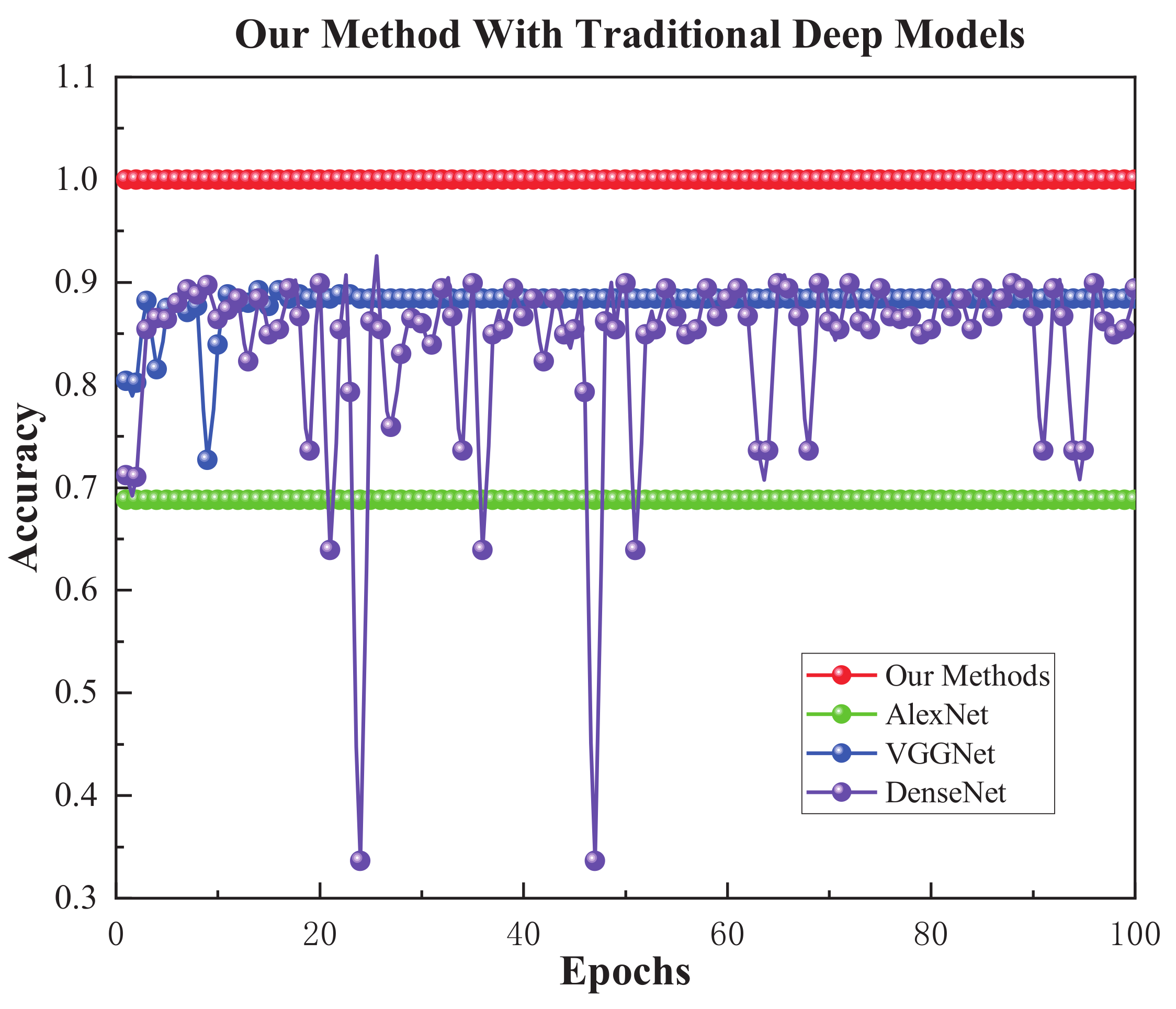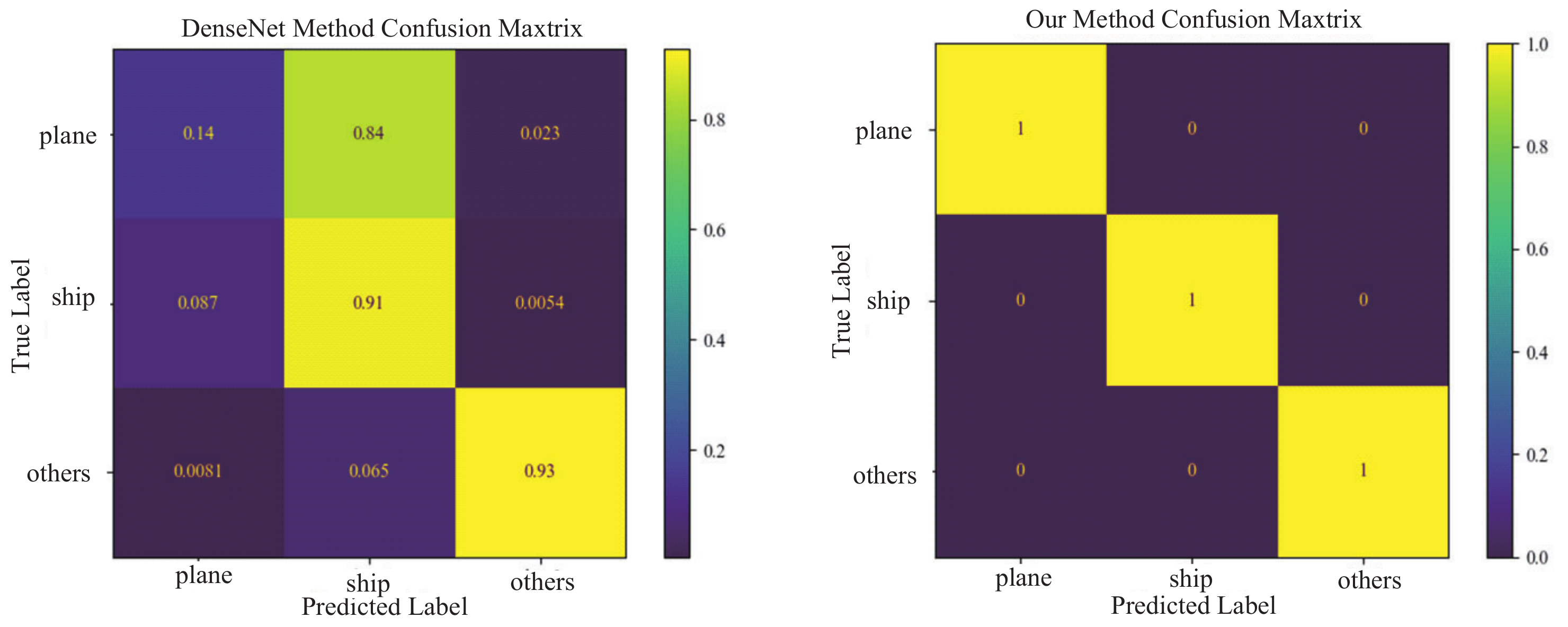In Section 4, the proposed approach is compared to classical DL algorithms, and the accuracy, precision, recall, F1, and other indicators are analyzed. At the same time, the proposed method is compared to various TL networks in terms of the recognition rate.

3. Materials and Methods

3.1. SSS Image Style Transfer for Optical Images

3.1.1. Image Encoding–Decoding Reconstruction Model

Style transfer is a crucial image-editing technique that enables new works of art to be created [36] and can be employed to generate SSS-style images from optical ones. Its purpose is to transform an image’s style without changing its content so that it has similar characteristics to the SSS images (signal-to-noise ratio, definition, resolution). Related work by Gatys et al. showed that the Gram matrix between features extracted using deep neural networks can capture image style information [36,37,38]. SSS-style image data can thus be obtained by minimizing a Gram-matrix-based loss function. This paper adopted a style-independent SSS image style transformation method based on the encoding–decoding model. In essence, the image style transformation method is an image reconstruction process. The traditional image reconstruction process (encoding–decoding) is shown in Figure 1. The loss function of the reconstruction is Equation (1), where $I_{in}$ is the input image, $I_{out}$ is the reconstructed image, and $\phi$ is the encoded features extracted using the deep network.

$$L={∥I_{in}-I_{out}∥}_2^2+\lambda {∥\phi \left(I_{in}\right)-\phi \left(I_{out}\right)∥}_2^2$$

(1)

3.1.2. Image Content Information Extraction

In order to remove only the style information from the image and keep only the content information (contour, texture, and others) of the image, in this paper, a whitening transformation method was adopted to remove the style-related information in the image. During the process of synthetic image generation, considering that the decoder module in the encoder–decoder model must perform many deconvolution operations, the network model should be reused in the process of image style transfer, so the network structure does not require intra-layer connections. At the same time, considering the ability of the number of network layers to extract image features, this paper chose VGG19, which has more network layers in the VGGNet model, as the network model for the synthetic data.

Given a content image $I_c$ (the optical image) and a style image $I_s$ (the SSS image), the feature vectors $f_c\in {\Re }^{C\times H_c{W}_c}$ and $f_s\in {\Re }^{C\times H_s{W}_s}$ are first extracted from the images using VGGNet, where $H_c$, $H_s$ and $W_c$, $W_s$ are the heights and widths of the content and style image features, respectively, and C is the number of channels in the image. $f_c\in {\Re }^{C\times H_c{W}_c}$ and $f_s\in {\Re }^{C\times H_s{W}_s}$ are such that, if they are input into a decoding network, the original content image $I_c$ and style image $I_s$ will be restored.

Adding a whitening transformation method in the encoding–decoding network can preserve the content information in the image and reduce the style information. Since the style information is represented in the correlation between channels, removing the image style information reduces the channel correlation. Therefore, $f_c$ is transformed through correlation transformation, where the non-diagonal elements of the correlation matrix of the transformed features are transformed to 0 and the diagonal elements are transformed to 1 to retain the content information and remove the style information. The method adopted was to transform $f_c$, so that the transformed feature vector $f_{cafter}$ is irrelevant, i.e., $f_{cafter}{f_{cafter}}^T=I$.

In order to remove the noise interference of the extracted feature of $f_c$, $f_c$ was preprocessed by subtracting the mean $m_c$. Then, the matrix $D_c$ is defined as a diagonal matrix composed of the eigenvalues of the covariance matrix $f_c{f_c}^T\in {\Re }^{C\times C}$ and $E_c$ as the orthogonal matrix of the corresponding eigenvectors, satisfying $f_c{f_c}^T=E_c{D}_c{E_c}^T$. The whitening transformation process is shown in Equation (2).

$$f_{cafter}=E_c{D}_c^{-\frac{1}{2}}{E_c}^T{f}_c$$

(2)

The relevant derivation process is as follows:

$$\begin{array}{cc}\hfill f_{cafter}{f_{cafter}}^T& =\left(E_c{D}_c^{-\frac{1}{2}}{E_c}^T{f}_c\right){\left(E_c{D}_c^{-\frac{1}{2}}{E_c}^T{f}_c\right)}^T=E_c{D}_c^{-\frac{1}{2}}{E_c}^T{f}_c{f_c}^T{E}_c{D}_c^{-\frac{1}{2}}{E_c}^T\hfill \\ \hfill & =E_c{D}_c^{-\frac{1}{2}}{E_c}^T{E}_c{D}_c{E_c}^T{E}_c{D}_c^{-\frac{1}{2}}{E_c}^T=I\hfill \end{array}$$

(3)

The features can be changed into a diagonalized covariance matrix using Equation (3). This process removes, to a large extent, the information related to the style and retains the content information.

3.1.3. Image Style Information Transfer

Image style transfer transfers the application of the SSS sonar image style to an optical image that has undergone a whitening transformation so that the obtained image has the style characteristics of the SSS image while retaining its content information. The above correlation analysis shows that the style transfer can be quantified using the Gram matrix, which is a correlation matrix between the feature channels and the image channels and describes the style information of an image. $f_{cafter}$ is transformed so that the Gram matrix of the transformed features is equal to the Gram matrix of the style features. This results in a transformed image acquiring the style of the image. Therefore, by designing a style transformation method, the whitening feature vector $f_{cafter}$ will be transformed into $f_{cafter-s}$, which is equal to the Gram matrix of the style feature vector $f_s$, thus changing and applying the required SSS style features to the image. This is expressed mathematically through the condition $f_{cafter-s}{f_{cafter-s}}^T=f_s{f_s}^T$.

Similarly, before style transformation, the style features $f_s$ are turned into zero-mean by subtracting the mean $m_s$. The style transformation process is shown in Equation (4).

$$f_{cafter-s}=E_s{D}_s^{\frac{1}{2}}{E_s}^T{f}_{cafter}$$

(4)

where $D_s$ is a diagonal matrix composed of the eigenvalues of the covariance matrix $f_s{f_s}^T\in {\Re }^{C\times C}$ and E is the orthogonal matrix of the corresponding eigenvectors, satisfying $f_s{f_s}^T=E_s{D}_s{E_s}^T$. The relevant derivation process is as follows:

$$\begin{array}{cc}\hfill f_{cafter-s}{f_{cafter-s}}^T& =\left(E_s{D}_s^{\frac{1}{2}}{E_s}^T{f}_{cafter}\right){\left(E_s{D}_s^{\frac{1}{2}}{E_s}^T{f}_{cafter}\right)}^T\hfill \\ \hfill & =E_s{D}_s^{\frac{1}{2}}{E_s}^T{f}_{cafter}{f_{cafter}}^T{E}_s{D}_s^{\frac{1}{2}}{E_s}^T\hfill \end{array}$$

(5)

Since $f_{cafter}{f_{cafter}}^T=I$ and ${E_s}^T{E}_s=I$, Equation (5) can be rewritten as Equation (6).

$$f_{cafter-s}{f_{cafter-s}}^T=E_s{D}_s^{\frac{1}{2}}{E_s}^T{f}_{cafter}{f_{cafter}}^T{E}_s{D}_s^{\frac{1}{2}}{E_s}^T=E_s{D}_s{E_s}^T=f_s{f_s}^T$$

(6)

It is evident from Equation (6) that the feature vector $f_{cafter-s}$ after the style transfer transformation and the style image feature $f_s$ have the same Gram matrix, and $f_{cafter-s}$ can be used to restore the image through the image reconstruction network to achieve the transformation of the image style. Finally, $f_{cafter-s}$ is restored to its original mean, i.e., $f_{cafter-s}=f_{cafter-s}+m_s$.

This paper adopted the VGG19 network as the encoder (feature extraction) and the inverse VGG19 network as the decoder (image reconstruction). The encoding–decoding network was trained through the optical dataset, and the loss function used is Equation (1). This paper adopted a linear transformation method of feature addition (the WST) to the encoding–decoding network. In this way, the SSS image style transfer is performed on the optical image, and the transformed features have Gram matrix invariance. Therefore, in the style transfer process, once the network is trained to perform image reconstruction, the parameters of the encoder–decoder network do not need to be adjusted. The detailed process is shown in Figure 2. Finally, Equation (7) is employed to adjust the balance of the transferred style and the content features, where $\alpha \in [0,1]$ is the style control factor. The formula indicates that, with the increase in $\alpha$, the composite image tends to be more in the style of the SSS image. In this paper, the covariance matrix difference between the synthetic image and the style image was applied to evaluate the quality of the synthetic image. This paper selected the $\alpha$ value with the highest quality of the synthesized image.

$$f_{cafter-s}=\alpha f_{cafter-s}+(1-\alpha )f_c$$

(7)

3.1.4. WST Multi-Feature Layer Sequential Image Style Transfer

Figure 2 demonstrates that adding the WST in the middle of the encoder–decoder network results in the style transformation of the image. In order to further improve the ability of the style transfer, the transformed features are the deepest, and the WST is applied to multiple feature layers. This multi-level method can utilize the deep and shallow features of the encoder–decoder network, and the generated SSS-style images have better visual quality.

The VGG19 network used in this paper can be divided into five feature extraction sub-blocks based on each network layer. Similarly, the inverse VGG19 network also has five inverse feature sub-blocks. The WST is applied before each inverse feature sub-block. Figure 3 depicts the addition process.

Figure 3a indicates that the five feature layers $VGGEncoder\left(n\right)(n=1,2,3,4,5)$ of VGG19 perform feature extraction on the image sequentially. As the network layers deepen, the feature extraction takes place at finer levels of detail, and the extracted features are more detailed and abstract.

First, the WST is added to $VGGEncoder\left(n\right)(n=1,2,3,4,5)$ and $VGGDecoder\left(n\right)$$(n=5,4,3,2,1)$, and a synthetic image $I_n(n=5,4,3,2,1)$ is generated based on the content and style images, as illustrated in Figure 3b. Then, $I_n$ is passed as a content image and style image through $VGGEncoder(n-1)(n=1,2,3,4,5)$, the WST, and $VGGDecoder(n-1)$$(n=5,4,3,2,1)$ to generate the composite image $I_{n-1}(n=5,4,3,2,1)$. The final style transfer image is obtained iteratively. Because the features extracted by $VGGEncoder\left(n\right)$ become more local as n increases, so $I_5\to I_1$, the style transfer of the images progressively expands from a local to a global level. Thus, the synthesized images finally obtained are of good quality.

3.2. Multi-Modal Multi-Stage Transfer Network for Object Recognition

The classic ResNet152 network structure is deep, and the number of network parameters to be calculated is large. In order to avoid overfitting, a large number of training samples are required to optimize the network parameters. The ImageNet dataset includes 1,000,000 training samples and is utilized for training ResNet152. However, the number of samples included in the SSS dataset employed in the current study is less than one-thousandth of that of ImageNet, and it is insufficient to train ResNet152 fully from scratch, as this will result in poor results. With the application of DL in fields that lack a large number of training samples, TL has gradually become a popular solution to deal with the lack of training samples. Figure 4 displays the target recognition structure used for TL. First, after the network is trained on a large-scale optical image dataset, the model can be immediately applied to classify more than 1000 commonly used target categories. Then, the backbone network in the network structure is frozen, and the head network in the network structure is trained using underwater SSS images to achieve the SSS image target identification.

However, as noted in Challenge 1 in the previous section, for the classification of underwater SSS images, models pre-trained on optical images cannot achieve satisfactory results due to the significant difference between SSS images and optical images and the minimal size of the sonar image dataset used for training. Therefore, in this paper, different DL-based model network feature layers were trained using the optical, synthetic, real SAR, and SSS datasets. From the perspective of the number of samples in the dataset, the ImageNet dataset has about 1.2 million samples, the synthetic dataset about 20,000 samples, the SAR dataset about 9000 samples, and the SSS dataset about 1100 samples. Hence, this article trained duringthe process, and the network was trained in stages by adopting the dataset usage strategy with the number of samples from large to small to achieve the process of network transfer from a large sample dataset to small sample dataset and to solve the problem of the low recognition rate caused by insufficient sample data. From the perspective of data quality, ImageNet’s data quality is superior to the synthetic, SAR, and SSS datasets. Using the dataset strategy presented in this paper can allow the network to gradually adapt to changes in data quality. The problem of transfer learning failure caused by the difference between the optical and SSS dataset sample was solved. The feature layer of the network pre-trained using the optical dataset can extract basic features. The layer trained using the synthetic dataset has an improved ability to extract target features from a noisy background. The layer trained with the SAR dataset has the strongest ability to extract features under the background of interference because noise interference in SAR data is strong. Finally, the SSS dataset was used to train the remaining part of the network. The parameters of multiple models learned from the different modalities were transferred to the classification model of the SSS images for better low-level and high-level feature extraction and representation. The detailed multi-modal and multi-stage migration process is revealed in Figure 5. The details of the network training strategies are shown in

Table 1. ResNet152 transfer learning network training strategies.

	Subnetwork	Subnetwork_1	Subnetwork_2	Subnetwork_3	Subnetwork_4
Usage Step/Datasets
Step 1/ImageNet		Train	Train	Train	Train
Step 2/Synthetic Data		Freeze	Train	Train	Train
Step 3/SAR		Freeze	Freeze	Train	Train
Step 4/SSS		Freeze	Freeze	Freeze	Train

.

Figure 5 indicates the method of the network feature layer training applied in stages. Each training link adopted the cross-entropy loss function as the objective function (Equation (8)). The network was sequentially trained from shallow to deep, so that its ability to extract target features and resist noise improved gradually, and its recognition performance improved.

$$L=\frac{1}{N}\sum _i{L}_i=-\frac{1}{N}\sum _i\sum _c^M{y}_{ic}log\left(p_{ic}\right)$$

(8)

where M is the number of categories; $y_{ic}$ is a sign function (0 or 1), where if the true class of sample i is equal to c, $y_{ic}=1$, otherwise $y_{ic}=0$; $p_{ic}$ is the probability that the predicted sample i belongs to category c.

4. Experiments

This section presents the test results of the multi-modal staged SSS target recognition method based on style transfer. The experiments were run on a Microsoft Windows 10 operating system with an NVIDIA GTX TITAN-XP GPU and 64 GB of memory. Python Version 3.6.8 was used to design the network structure. This part verifies the robustness and effectiveness of the proposed method through comparative experiments and analysis. The method was compared to traditional DL recognition methods to verify the improvement effect of the algorithm on the recognition rate. In addition, this algorithm was compared to related TL algorithms, and the positive effect of the style target generation method adopted in this paper on target recognition was analyzed.

4.1. Experimental Settings

4.1.1. Application Dataset

A target image dataset collected via imaging sonar was employed to conduct the experiments (https://toscode.gitee.com/wangjian19870118/ssd-dataset.git accessed on 27 January 2023). The dataset used in the experiment includes three image targets: planes, ships, and others. The dataset comprises 66 plane pictures, 484 ship pictures, and 578 other pictures. Some example dataset images are shown in Figure 6. It can be seen that the images have strong noise interference, which causes great difficulty in accurately identifying the target.

4.1.2. Experimental Dataset Preprocessing

Random extraction was conducted for each image type, where 70% of the data were used for training data and 30% for testing. Table 1 lists the specific data allocation for each category. In order to reduce the influence of the random initialization of the parameters and the random sampling of the samples on the recognition effect, the average values of repeated experiments were used for the final evaluation of the recognition effect. The data types in the dataset were unbalanced, with the largest being the 578 other samples and only 66 plane samples. Unbalanced data will cause the classifier to favor categories with large sample sizes, and the recognition rate of small sample categories will be poor. At the same time, the total number of samples in the dataset was 1128, and the network trained using this dataset exhibited overfitting. In this experiment, to reduce the above problems’ impact on the algorithm, some basic data enhancement methods (flipping, rotation, cropping) were also applied to preprocess the data. These included cropping (center, bottom-left, top-left, bottom-right, top-right), equal-height or -width stretching, contrast transformations, rotation (45${}^{\circ }$, 90${}^{\circ }$, 135${}^{\circ }$, 180${}^{\circ }$, 225${}^{\circ }$, 270${}^{\circ }$, and 315${}^{\circ }$), and left and right flipping. Figure 7 depicts the image transformation result. Figure 8 shows the image data used in the experiment. It indicates that different types of images have different appearances and distributions.

4.2. Evaluation Metrics

The criteria for evaluating the model performance adopted in this paper were the accuracy, precision, and recall. The calculation method of the above evaluation criteria is described in

Table 2. Evaluation metrics of the algorithm.

		Prediction		Total
		1	0
Actual	1	True Positive (TP)	True Negative (FN)	Actual Positive (TP + FN)
	0	False Positive (FP)	False Negative (TN)	Actual Negative (FP + TN)
Total		Predicted Positive (TP + FP)	Predicted Negative (FN + TN)	(TP + FN + FP + TN)

:

TP:

If a sample belongs to a specific class, and is predicted as such, this is considered a true positive outcome.

TN:

If a sample does not belong in a class, and is predicted not to belong, this is considered a true negative outcome.

FP:

If a sample does not belong to a class, but is predicted to, then this is considered a false positive outcome.

FN:

If a sample belongs to a class, but is predicted not to, this is considered a false negative.

The problem tackled in this paper involved the classification into multiple categories. Since the above indicators only apply to binary classification problems, they were applied separately to each category to evaluate the proposed algorithm.

Accuracy: the ratio of correctly predicted samples to the total sample number.

$$accuracy=\frac{\mathrm{TP}+\mathrm{TN}}{\mathrm{TP}+\mathrm{TN}+\mathrm{FP}+\mathrm{FN}}$$

Precision: the ratio of the number of samples correctly predicted to be positive to the number of samples predicted to be positive.

$$precision=\frac{\mathrm{TP}}{\mathrm{TP}+\mathrm{FP}}$$

Recall rate: the ratio of the number of samples correctly predicted to be positive to the total number of positive samples.

$$recall=\frac{\mathrm{TP}}{\mathrm{TP}+\mathrm{FN}}$$

4.3. Performance Analysis

The network presented in this paper employed the ResNet152 network as its basis. The ImageNet, synthetic, and SAR images were used, respectively, to train the front section, middle section, and back-end of the backbone network, while the SSS images were utilized for training the head of the network. The batch size was set to 100 and the learning rate to 0.001. The VGG19 network was used for image style transfer to generate a synthetic dataset with a learning rate of 0.001 and a batch size of 50.

Model validation was performed ten times using the cross-validation method, and the average value of each performance indicator in the test dataset was used as the final recognition effect measurement:

(1)

Comparison of our method with traditional DL models:

In order to analyze the method’s performance in terms of the recognition accuracy, a comparison was conducted with the traditional AlexNet, VGGNet, and DenseNet methods. These three methods are the most-commonly used backbone structures in SSS target recognition [13,14]. VGGNet has more network layers than AlexNet, and DenseNet’s structure is more complex than that of VGGNet. Comparing these three networks’ structures will help to evaluate the proposed method’s performance in terms of the network layers, the data used for training, and the network structures employed. Figure 9 demonstrates that the worst performance was that of the AlexNet algorithm, achieving less than a 70% recognition accuracy. The VGGNet and DesNet algorithms performed similarly at about a 89% accuracy, with DenseNet performing slightly better than VGGNet. The performance of the proposed method was substantially better, with a recognition accuracy of nearly 100%, and the identification curve was more consistent than the other two methods. To further analyze the algorithm’s performance, the precision and recall of the method in this paper and those of DenseNet, which had better performance than the other methods, were compared. The results are shown in

Table 3. Evaluation metrics between the proposed and the DenseNet methods.

	Precision	Recall	Accuracy
planeDenseNet	0.5386	0.5345	0.8672
shipDenseNet	0.8316	0.819	0.8523
othersDenseNet	0.9764	0.9597	0.9775
Our Method	1	1	1

, indicating that the proposed method’s precision and recall were higher than the related evaluation metrics of DenseNet.

In order to analyze the recognition effects of the proposed and DesNet methods on each of the three target categories, the confusion matrix was obtained (Figure 10), where class1 corresponds to plane, class2 to ship, and class3 to others.

(2)

Comparison of the methods for the classification of SSS images:

The proposed method was then compared to some improved algorithms used for SSS recognition. The above algorithms were trained using only the SSS dataset presented in this paper for underwater target recognition, and the synthetic style transfer dataset was not used. The results revealed that using synthetic datasets can improve the accuracy of target recognition.

Table 4. Comparison of different methods for SSS image object recognition.

Methods	Layer Number	Accuracy (%)
Shallow CNN [15]	11	83.19
GoogleNet [16]	22	91.86
VGG11 fine-tuning + semi-synthetic data [13]	11	92.51
VGG19 fine-tuning [14]	19	94.67
VGG19 fine-tuning + semi-synthetic data	19	97.76
SPDRDL [17]	46	97.38
FL-DARTS [18]	50	99.07
Ours	152	100

exhibits that, as the number of network layers increased, the recognition accuracy of the algorithms of [14,15,16] showed an upward trend, and their accuracy rose from 83.19% to 94.67%. The methods in [13,14,18] employed TL to identify the SSS target, and the recognition accuracy was significantly improved. The transfer learning method also had a positive effect on the recognition effect. Using semi-synthetic data samples for the TL-based target recognition increased the recognition accuracy rate from 94.67% to 97.76%, an increase of 3% points. The methods of [17,18] adopt self-supervised learning and empirical knowledge to improve the recognition accuracy of SSS images. The proposed method in this paper improved the target recognition performance through sample generation and modal transfer, and its performance was better than all the above methods.

(3)

Comparison of different backbones for the classification of SSS images:

In order to analyze the impact of different backbone networks on target recognition, different networks were combined with the fine-tuned head network to identify SSS targets.

Table 5. Comparison of TL-based SSS image target recognition with different backbone networks.

Backbone Networks	Accuracy (%)
AlexNet	94.14
GoogleNet	94.46
VGG16	94.5
VGG19	94.67
ResNet18	91.86
ResNet50	93.5
DenseNet	94.14

indicates that VGG19 had better generalization performance because it has more network layers than VGG16. Therefore, it was more suitable for generating SSS-style images in the image synthesis, indirectly improving the recognition performance.

(4)

Comparison of different TL strategies:

This paper adopted four TL strategies to identify the target and compare the performance of different modal image transfer strategies. The recognition results are shown in

Table 6. Comparison of multi-modal SSS image TL methods.

Dataset Training Order	Accuracy (%)
SAR	97.72
Optical	97.12
SAR + Optical	98.34
Optical + Synthetic Dataset + SAR + SSS (Our Method)	100

. Because the optical data characteristics were the most different from the SSS data distribution, the achieved recognition accuracy was only 97.12%. After introducing the SAR dataset, the robustness of the network to noise improved, with the recognition rate was increased by 1.2 percentage points, reaching 98.34%. Through image synthesis, the proposed method reduced the difference between the data distributions and, at the same time, improved the anti-noise performance of the network, thus achieving the best recognition effect.

(5)

Comparison of various backbones for classifying noisy SSS images:

Because a variety of noise interference often accompanies SSS images, in order to analyze the SSS target recognition performance under strong noise interference, in this paper, Gaussian, speckle, multiplicative, and Poisson noises were randomly added to the original SSS images. These are typical SSS image noises, which can simulate the underwater image under a strong noise environment. Since VGGNet, ResNet, and DenseNet are the most-classical and -widely used backbone network structures, the transfer recognition methods of these three backbone networks were selected as the comparison algorithm.

Table 7. Comparison of strongly noisy SSS image target recognition with different backbone networks.

Backbone Networks	Accuracy (%)
VGG	95.5
ResNet	92.68
DenseNet	91.63
Ours	95.92

exhibits the experimental results.

Figure 7 demonstrates that the recognition accuracy of the proposed method was 95.92%, while the recognition accuracy of DenseNet was the lowest at only 91.63%, and the recognition accuracy of VGG was the highest at 95.5%. The proposed method had a recognition accuracy higher than 0.42%, 3.24%, and 4.29%, respectively. This method has a good recognition effect under strong noise interference.

(6)

Application of FLS target recognition:

The proposed method can recognize SSS targets and be applied to FLS target recognition. In order to verify the effectiveness of the proposed approach in more categories of target recognition, this paper used Forward-Looking Sonar (FLS) data for the experiments. Among them, the total number of samples was 3192, the number of target categories 10, the number of training sets 2231, and the number of test sets 961. Figure 11 depicts the data sample diagram, whereas

Table 8. Comparison of different DL models for FLS image object recognition.

Methods	Optimal OA (%)
DenseNet201	89.07
DenseNet121	88.87
DenseNet169	89.91
ResNet50	89.49
ResNet101	88.14
ResNet152	88.03
VGGNet16	90.63
VGGNet19	85.22
Proposed	100

displays the experimental results.

Table 8 shows that the recognition rates of the DenseNet series of algorithms were DenseNet201 OA = 89.07, DenseNet121 OA = 88.87, and DenseNet201 OA = 89.91, which were slightly higher than the ResNet series of algorithms. The recognition rates of the DenseNet and ResNet algorithms were above 88%. VGGNet16 was the best, with OA = 90.63%, among the reference algorithms, and VGGNet19 was the worst, with OA = 85.22. The proposed method was superior to the compared algorithms. This showed that the proposed approach has a good effect on FLS target recognition.

5. Discussion

This paper solved the problem of the low recognition rates caused by the difference between the transfer domain samples and the target domain samples in the TL target recognition methods. A synthetic sample dataset was thus proposed to identify SSS targets and multi-dataset joint TL-based recognition.

5.1. Method Importance

The data synthesis method proposed in this paper provides a new approach to underwater target recognition. It is extremely useful as a recognition method when small amounts of class samples are available and acquiring additional samples is costly or dangerous.

The WST image transformation method was introduced, and the SSS style transfer was performed on optical data using an encoding–decoding model. This method reduces the problem of data source differences in target recognition and provides a solution and a new direction for TL-based underwater target recognition.

The deep network multi-modal migration strategy is introduced in stages so that the recognition model can extract deeper feature information as the number of network layers continues to increase. This approach was adopted because the signal-to-noise ratio of the dataset used was reduced, so the extracted features needed strong noise robustness.

5.2. Algorithm Limitations

The proposed method achieved good performance in the experiment, but the number of data sample categories was small, while the effect of target recognition will decrease as this number increases. At the same time, there are many kinds of targets in underwater environments, including airplanes and ships, and many smaller objects. Therefore, a deep network model that can extract stronger discriminative features is required.

In addition, the datasets used in this paper are suitable for supervised training. The recognition effect of the proposed method will decline when training sets suitable for weak supervision are used.

Because there is a large amount of unlabeled data in the weakly supervised training dataset, making the sample size of the original SSS dataset comparably smaller, in the process of network training, the recognition rate of the training data was high. However, the recognition accuracy on the test dataset reduced, indicating that overfitting occurred. At the same time, the proposed method’s network parameters are large, and the above problems are more likely to occur. Therefore, there is still room for improvement of the proposed method by adopting semi-supervised training methods. A network trained in a semi-supervised manner can learn the parameters of the unsupervised network through the unlabeled data in the limited training dataset and use the labeled data for fine-tuning, improving the semi-supervised target recognition effect.

6. Conclusions

The performance of TL-based SSS target recognition methods frequently suffers when there are substantial differences in the characteristics of the source and target domain training data and from the high noise interference of SSS images, which negatively impacts the feature extraction capability of the recognition network. This study proposed a dataset synthesis method based on image style transfer. The method generates data samples with an SSS image style using optical data and reduces the difference between the data from the two modalities. Then, multiple datasets were used to train different sub-block feature layers of the network to improve the robustness of the feature extraction ability. The experimental results showed that the method can better identify sunken underwater ships, wrecked planes, and other targets. This study provides theoretical support for the accurate identification of more underwater targets. With the continuous addition of style images and the continuous improvement of data samples, the target recognition effect will be improved further.

References

1. Bhanu, B. Automatic target recognition: State of the art survey. IEEE Trans. Aerosp. Electron. Syst. 1986, AES-22, 364–379. [Google Scholar] [CrossRef]
2. Chaillan, F.; Fraschini, C.; Courmontagne, P. Speckle noise reduction in SAS imagery. Signal Process. 2007, 87, 762–781. [Google Scholar] [CrossRef]
3. Kazimierski, W.; Zaniewicz, G. Determination of process noise for underwater target tracking with forward looking sonar. Remote. Sens. 2021, 13, 1014. [Google Scholar] [CrossRef]
4. Wang, H.; Wang, B.; Li, Y. IAFNet: Few-shot learning for modulation recognition in underwater impulsive noise. IEEE Commun. Lett. 2022, 26, 1047–1051. [Google Scholar] [CrossRef]
5. Zhang, X.; Ying, W.; Yang, P.; Sun, M. Parameter estimation of underwater impulsive noise with the Class B model. IET Radar Sonar Navig. 2020, 14, 1055–1060. [Google Scholar] [CrossRef]
6. Li, H.; Dong, Y.; Gong, C.; Zhang, Z.; Wang, X.; Dai, X. A non-gaussianity-aware receiver for impulsive noise mitigation in underwater communications. IEEE Trans. Veh. Technol. 2021, 70, 6018–6028. [Google Scholar] [CrossRef]
7. Topple, J.M.; Fawcett, J.A. MiNet: Efficient deep learning automatic target recognition for small autonomous vehicles. IEEE Geosci. Remote. Sens. Lett. 2020, 18, 1014–1018. [Google Scholar] [CrossRef]
8. Lin, Z.; Ji, K.; Leng, X.; Kuang, G. Squeeze and excitation rank faster R-CNN for ship detection in SAR images. IEEE Geosci. Remote. Sens. Lett. 2018, 16, 751–755. [Google Scholar] [CrossRef]
9. Zhang, T.; Zhang, X.; Shi, J.; Wei, S. High-speed ship detection in SAR images by improved yolov3. In Proceedings of the 2019 16th International Computer Conference on Wavelet Active Media Technology and Information Processing, Chengdu, China, 13–15 December 2019; pp. 149–152. [Google Scholar]
10. Dobeck, G.J.; Hyland, J.C. Automated detection and classification of sea mines in sonar imagery. Proc. SPIE 1997, 3079, 90–110. [Google Scholar]
11. Wan, S.; Yeh, M.L.; Ma, H.L. An innovative intelligent system with integrated CNN and SVM: Considering various crops through hyperspectral image data. ISPRS Int. J. Geo-Inf. 2021, 10, 242. [Google Scholar] [CrossRef]
12. Çelebi, A.T.; Güllü, M.K.; Ertürk, S. Mine detection in side scan sonar images using Markov Random Fields with brightness compensation. In Proceedings of the 2011 IEEE 19th Signal Processing and Communications Applications Conference (SIU), Antalya, Turkey, 20–22 April 2011; pp. 916–919. [Google Scholar]
13. Ye, X.; Li, C.; Zhang, S.; Yang, P.; Li, X. Research on side-scan sonar image target classification method based on transfer learning. In Proceedings of the OCEANS 2018 Conference, Charleston, NC, USA, 22–25 October 2018; pp. 1–6. [Google Scholar]
14. Huo, G.; Wu, Z.; Li, J. Underwater object classification in sidescan sonar images using deep transfer learning and semisynthetic training data. IEEE Access 2020, 8, 47407–47418. [Google Scholar] [CrossRef]
15. Luo, X.; Qin, X.; Wu, Z.; Yang, F.; Wang, M.; Shang, J. Sediment classification of small-size seabed acoustic images using convolutional neural networks. IEEE Access 2019, 7, 98331–98339. [Google Scholar] [CrossRef]
16. Qin, X.; Luo, X.; Wu, Z.; Shang, J. Optimizing the sediment classification of small side-scan sonar images based on deep learning. IEEE Access 2021, 9, 29416–29428. [Google Scholar] [CrossRef]
17. Gerg, I.D.; Monga, V. Structural prior driven regularized deep learning for sonar image classification. IEEE Trans. Geosci. Remote. Sens. 2021, 60, 4200416. [Google Scholar] [CrossRef]
18. Zhang, P.; Tang, J.; Zhong, H.; Ning, M.; Liu, D.; Wu, K. Self-trained target detection of radar and sonar images using automatic deep learning. IEEE Trans. Geosci. Remote. Sens. 2021, 60, 4701914. [Google Scholar] [CrossRef]
19. Simonyan, K.; Zisserman, A. Very deep convolutional networks for large-scale image recognition. arXiv 2014, arXiv:1409.1556. [Google Scholar]
20. Krizhevsky, A.; Sutskever, I.; Hinton, G.E. Imagenet classification with deep convolutional neural networks. Commun. ACM 2017, 60, 84–90. [Google Scholar] [CrossRef] [Green Version]
21. He, K.; Zhang, X.; Ren, S.; Sun, J. Deep residual learning for image recognition. In Proceedings of the IEEE Conference on Computer Vision and Pattern Recognition, Las Vegas, NV, USA, 26 June–1 July 2016; pp. 770–778. [Google Scholar]
22. Xu, S.; Qiu, X.; Wang, C.; Zhong, L.; Yuan, X. Desnet: Deep residual networks for Descalloping of ScanSar images. In Proceedings of the IGARSS 2018—2018 IEEE International Geoscience and Remote Sensing Symposium, Valencia, Spain, 23–27 July 2018; pp. 8929–8932. [Google Scholar]
23. Wu, Z.; Shen, C.; Van Den Hengel, A. Wider or deeper: Revisiting the resnet model for visual recognition. Pattern Recognit. 2019, 90, 119–133. [Google Scholar] [CrossRef] [Green Version]
24. Qiu, C.; Zhou, W. A survey of recent advances in CNN-based fine-grained visual categorization. In Proceedings of the 2020 IEEE 20th International Conference on Communication Technology (ICCT), Nanning, China, 28–31 October 2020; pp. 1377–1384. [Google Scholar]
25. Fukushima, K.; Miyake, S.; Ito, T. Neocognitron: A neural network model for a mechanism of visual pattern recognition. IEEE Trans. Syst. Man Cybern. 1983, 13, 826–834. [Google Scholar] [CrossRef]
26. LeCun, Y. Generalization and network design strategies. Connect. Perspect. 1989, 19, 18. [Google Scholar]
27. Deng, J.; Dong, W.; Socher, R.; Li, L.J.; Li, K.; Fei-Fei, L. Imagenet: A large-scale hierarchical image database. In Proceedings of the 2009 IEEE Conference on Computer Vision and Pattern Recognition, Miami, FL, USA, 20–15 June 2009; pp. 248–255. [Google Scholar]
28. He, K.; Girshick, R.; Dollár, P. Rethinking imagenet pre-training. In Proceedings of the IEEE/CVF International Conference on Computer Vision, Seoul, Republic of Korea, 11–17 October 2019; pp. 4918–4927. [Google Scholar]
29. Zhao, L.; Li, S. Object detection algorithm based on improved YOLOv3. Electronics 2020, 9, 537. [Google Scholar] [CrossRef] [Green Version]
30. Xu, X.; Zhao, M.; Shi, P.; Ren, R.; He, X.; Wei, X.; Yang, H. Crack detection and comparison study based on faster R-CNN and mask R-CNN. Sensors 2022, 22, 1215. [Google Scholar] [CrossRef] [PubMed]
31. Yulin, T.; Jin, S.; Bian, G.; Zhang, Y. Shipwreck target recognition in side-scan sonar images by improved YOLOv3 model based on transfer learning. IEEE Access 2020, 8, 173450–173460. [Google Scholar] [CrossRef]
32. Ji-yang, Y.; Dan, H.; Lu-yuan, W.; Xin, L.; Wen-juan, L. On-board ship targets detection method based on multi-scale salience enhancement for remote sensing image. In Proceedings of the 2016 IEEE 13th International Conference on Signal Processing (ICSP), Chengdu, China, 6–10 November 2016; pp. 217–221. [Google Scholar]
33. Ren, S.; He, K.; Girshick, R.; Sun, J. Faster R-CNN: Towards real-time object detection with region proposal networks. In Proceedings of the 28th International Conference on Neural Information Processing Systems (NIPS’15), Montreal, QC, Canada, 7–12 December 2015; Volume 28. [Google Scholar]
34. Chandrashekar, G.; Raaza, A.; Rajendran, V.; Ravikumar, D. Side scan sonar image augmentation for sediment classification using deep learning based transfer learning approach. Mater. Today Proc. 2021. [Google Scholar] [CrossRef]
35. Ge, Q.; Ruan, F.; Qiao, B.; Zhang, Q.; Zuo, X.; Dang, L. Side-scan sonar image classification based on style transfer and pre-trained convolutional neural networks. Electronics 2021, 10, 1823. [Google Scholar] [CrossRef]
36. Li, Y.; Fang, C.; Yang, J.; Wang, Z.; Lu, X.; Yang, M.H. Diversified texture synthesis with feed-forward networks. In Proceedings of the IEEE Conference on Computer Vision and Pattern Recognition, Honolulu, HI, USA, 21 July–26 July 2017; pp. 3920–3928. [Google Scholar]
37. Gatys, L.A.; Ecker, A.S.; Bethge, M. Image style transfer using convolutional neural networks. In Proceedings of the IEEE Conference on Computer Vision and Pattern Recognition, Las Vegas, NV, USA, 26 June–1 July 2016; pp. 2414–2423. [Google Scholar]
38. Gatys, L.; Ecker, A.S.; Bethge, M. Texture synthesis using convolutional neural networks. Adv. Neural Inf. Process. Syst. 2015, 28. [Google Scholar]
Figure 1. Image encoder–decoder reconstruction model structure diagram.
Remotesensing 15 01303 g001
Figure 2. Illustration of image encoder–decoder style transfer.
Remotesensing 15 01303 g002
Figure 3. Illustration of WST multi-feature layer sequence image style transfer: (a) VGG19 network structure diagram; (b) WST process details and multi-feature layer addition.
Remotesensing 15 01303 g003
Figure 4. Basic model of TL-based object recognition.
Remotesensing 15 01303 g004
Figure 5. Structure diagram of multi-mode multi-stage transmission network for object recognition.
Remotesensing 15 01303 g005
Figure 6. Side-scan sonar dataset samples: (a) three classes of side-scan image targets; (b) sample distribution diagram.
Remotesensing 15 01303 g006
Figure 7. Image transformation result graph: (a) image sample; (b) center crop; (c) bottom-left crop; (d) top-left crop; (e) bottom-right crop; (f) top-right crop; (g) equal-height stretch; (h) equal-width stretch; (i) contrast transformation (gamma = 0.87); (j) contrast transformation (gamma = 1.07); (k) rotation by 45 ; (l) rotation by 90 ; (m) rotation by 135 ; (n) rotation by 180 ; (o) rotation by 225 ; (p) rotation by 270 ; (q) rotation by 315 ; (r) left and right flip.
Remotesensing 15 01303 g007
Figure 8. The datasets used in the experiments: (a) grayscale optical image samples; (b) synthetic image samples; (c) SAR image samples; (d) SSS image samples.
Remotesensing 15 01303 g008
Figure 9. Result graph comparing the proposed method with the traditional ones.
Remotesensing 15 01303 g009
Figure 10. Confusion matrix result graph between the proposed method and DesNet.
Remotesensing 15 01303 g010
Figure 11. Forward-looking sonar dataset samples’ diagram.
Remotesensing 15 01303 g011