
Interannual Variation of Landfast Ice Using Ascending and Descending Sentinel-1 Images from 2019 to 2021: A Case Study of Cambridge Bay

Abstract
:1. Introduction
2. Methods
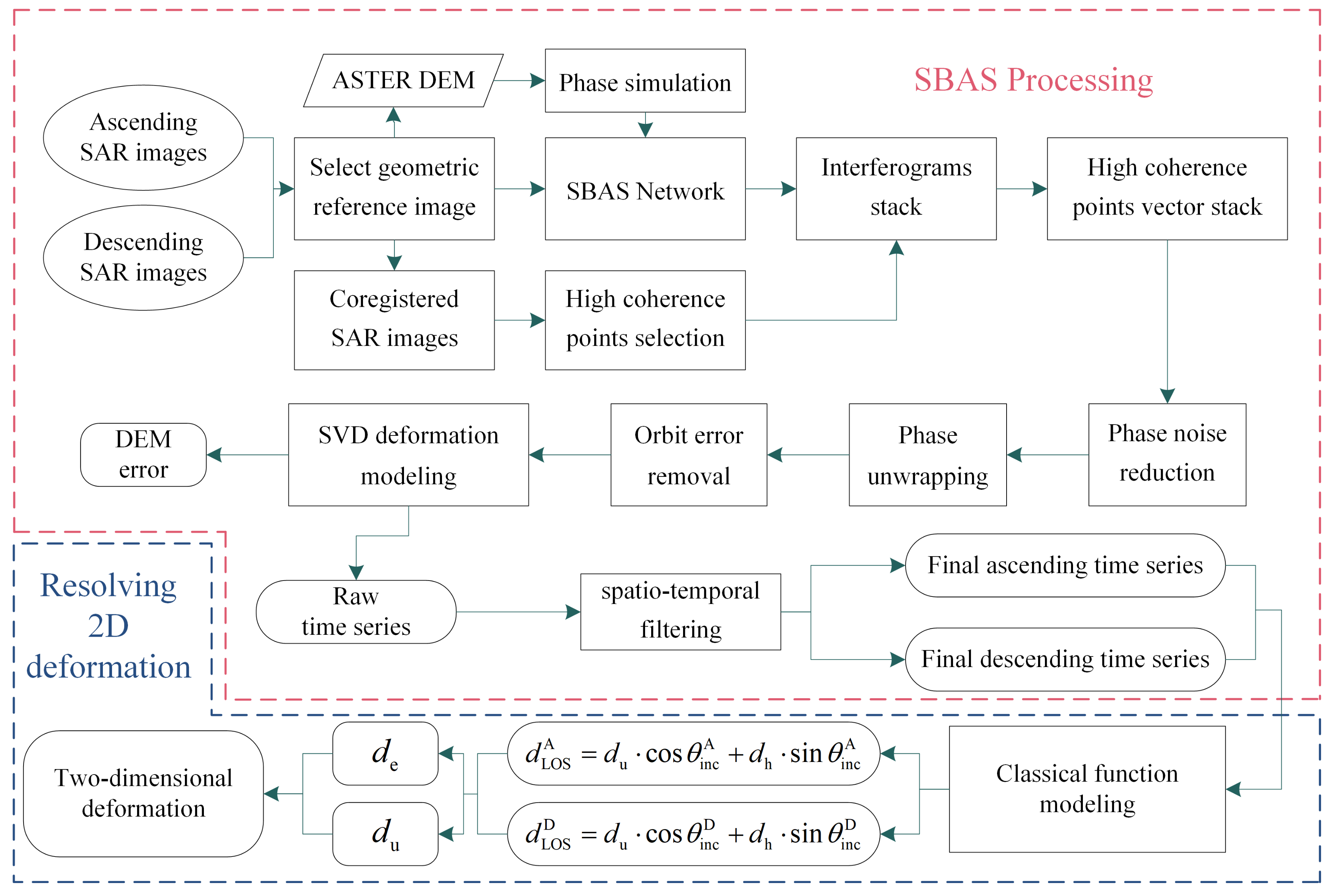
2.1. SBAS-InSAR Data Processing
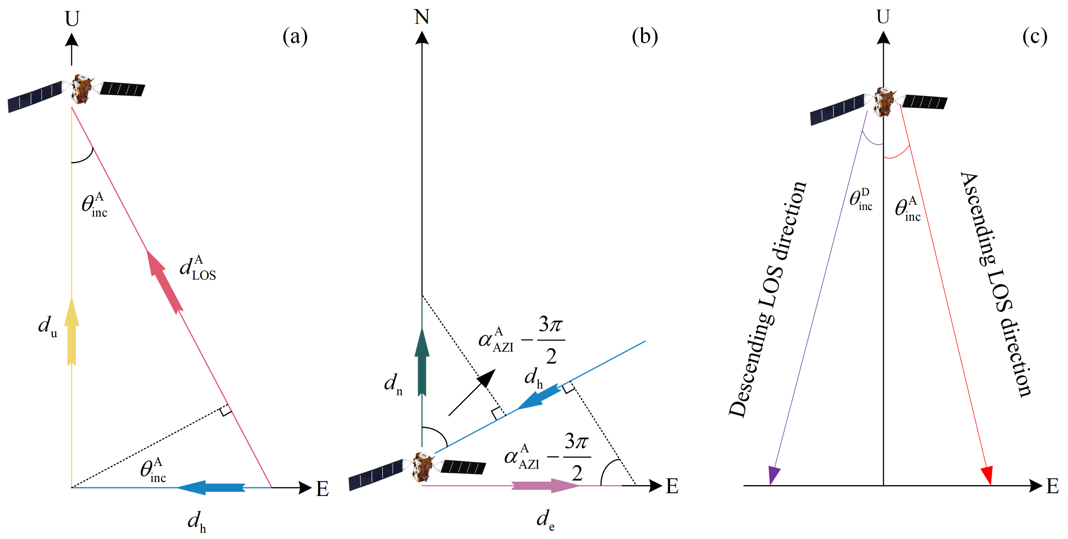
2.2. Calculation of Horizontal and Vertical Deformations
3. Study Area and Datasets
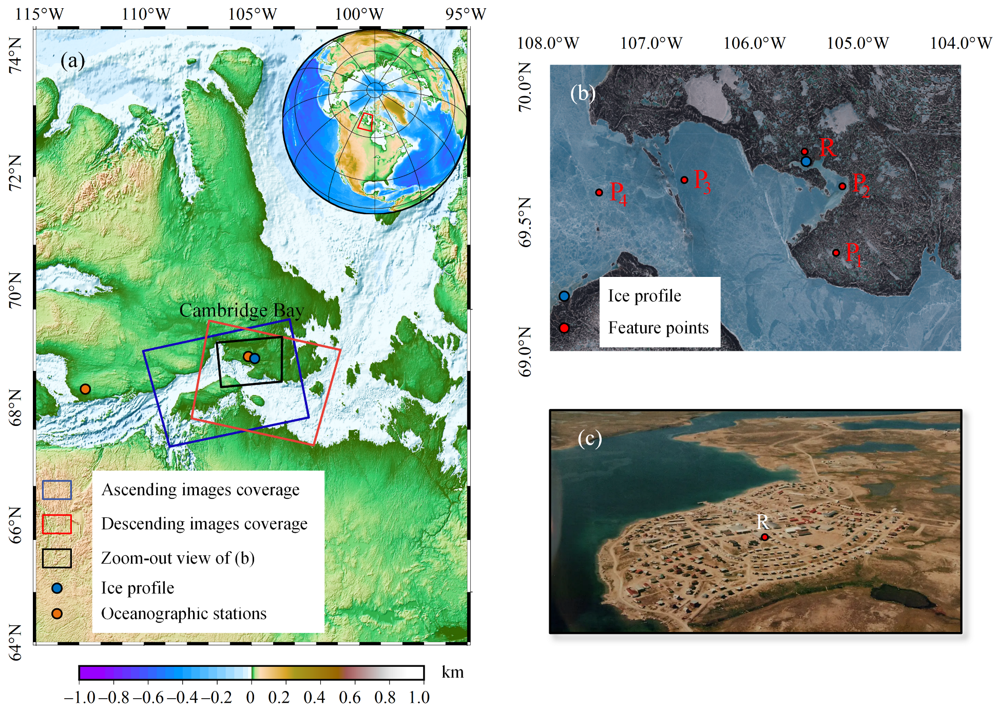
3.1. Cambridge Bay
3.2. Sentinel-1 Images and Reference Data
4. Results
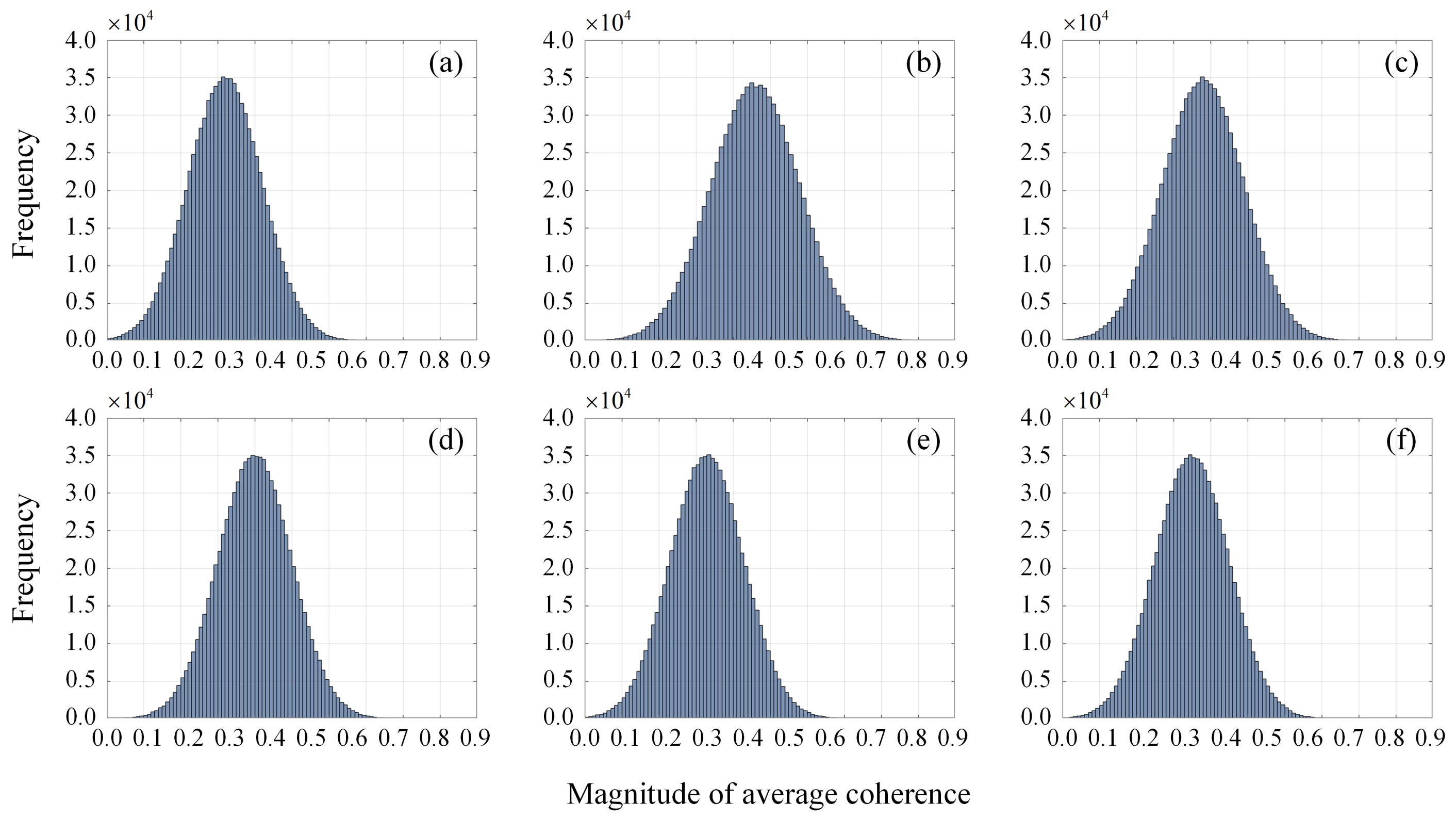
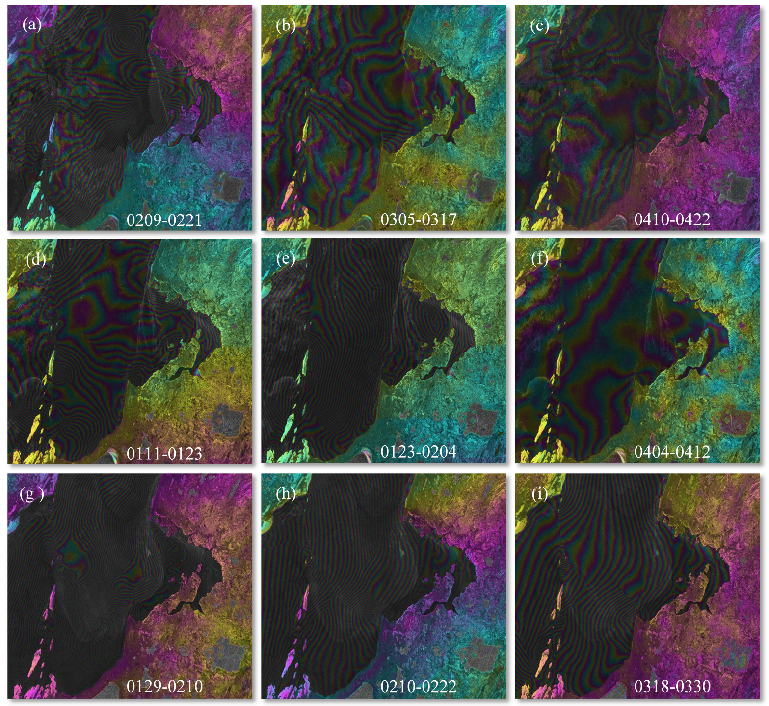
4.1. Average Coherence and Interferograms
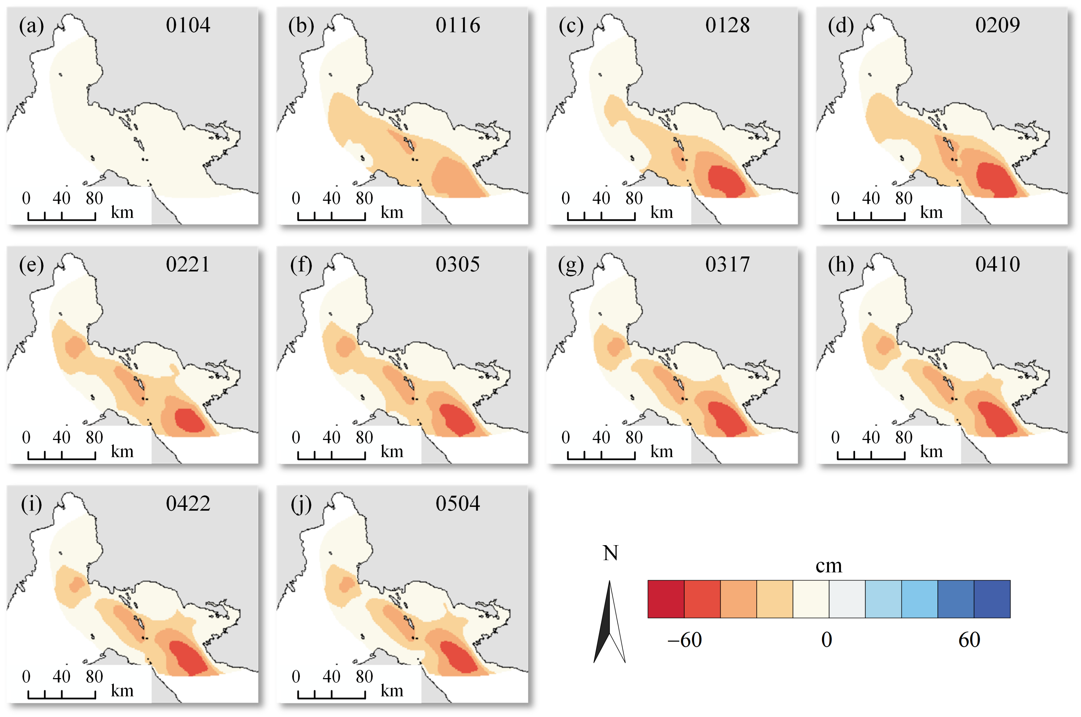
4.2. Ascending and Descending LOS Deformations
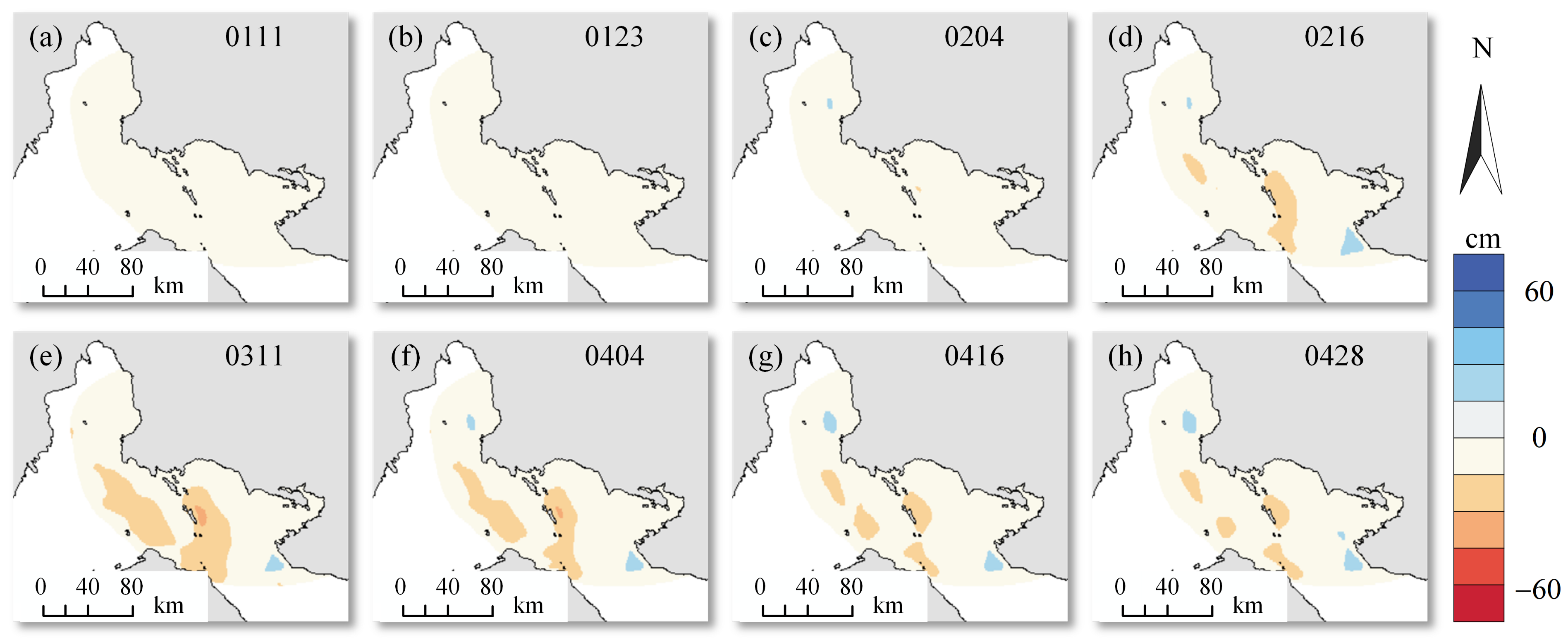
4.3. Horizontal and Vertical Deformations
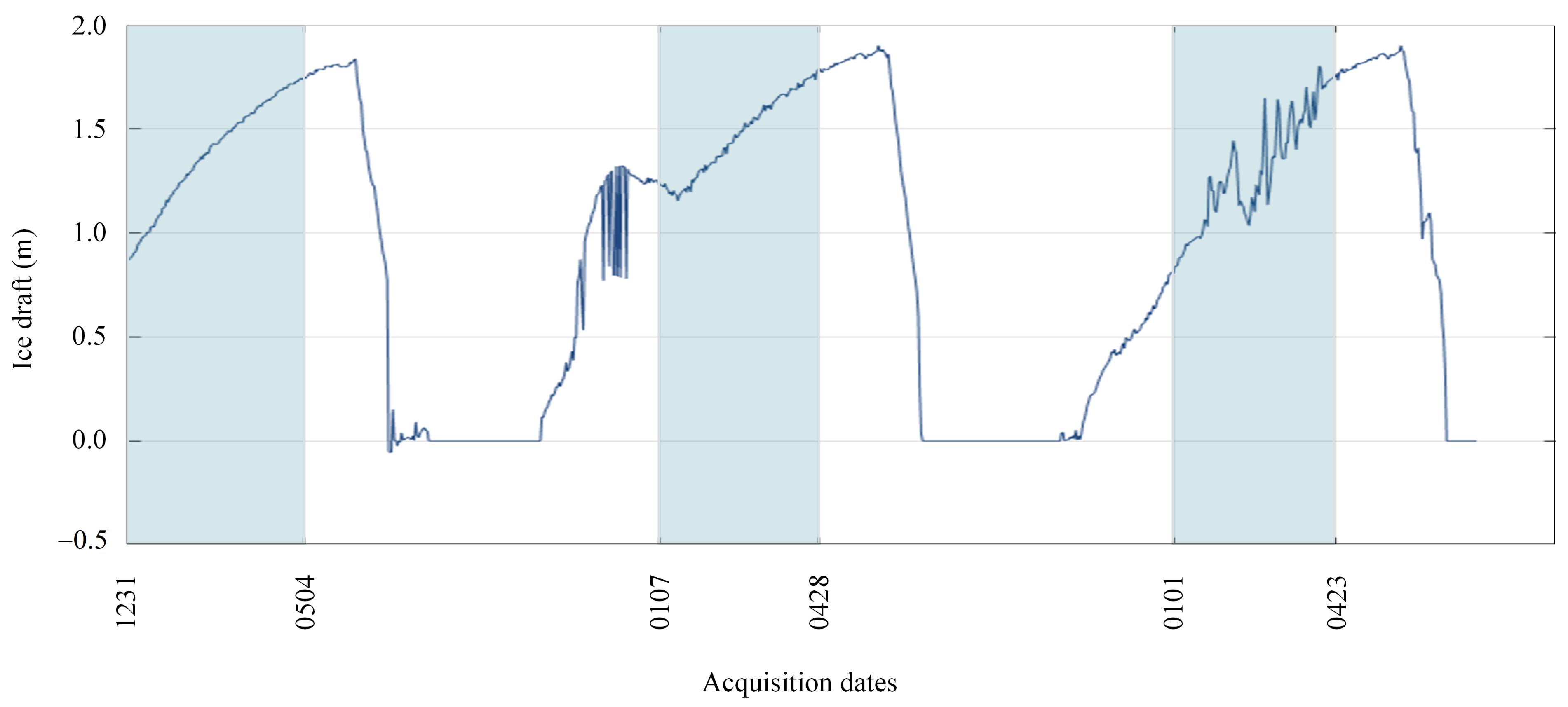
4.4. Validation
5. Discussion
5.1. Suggested Reasons for Deformation
5.2. Possible Causes of Interannual Variation
6. Conclusions
Author Contributions
Funding
Data Availability Statement
Acknowledgments
Conflicts of Interest
Appendix A

| Acquisition Date | Sensor | Flight Direction | Acquisition Date | Sensor | Flight Direction |
|---|---|---|---|---|---|
| 20181231 | S1A | Descending | 20200216 | S1B | Ascending |
| 20190104 | S1B | Ascending | 20200307 | S1A | Descending |
| 20190112 | S1A | Descending | 20200311 | S1B | Ascending |
| 20190116 | S1B | Ascending | 20200331 | S1A | Descending |
| 20190124 | S1A | Descending | 20200404 | S1B | Ascending |
| 20190128 | S1B | Ascending | 20200412 | S1A | Descending |
| 20190205 | S1A | Descending | 20200416 | S1B | Ascending |
| 20190209 | S1B | Ascending | 20210101 | S1A | Descending |
| 20190217 | S1A | Descending | 20210105 | S1B | Ascending |
| 20190221 | S1B | Ascending | 20210113 | S1A | Descending |
| 20190301 | S1A | Descending | 20210117 | S1B | Ascending |
| 20190305 | S1B | Ascending | 20210125 | S1A | Descending |
| 20190313 | S1A | Descending | 20210129 | S1B | Ascending |
| 20190317 | S1B | Ascending | 20210206 | S1A | Descending |
| 20190325 | S1A | Descending | 20210210 | S1B | Ascending |
| 20190410 | S1B | Ascending | 20210218 | S1A | Descending |
| 20190406 | S1A | Descending | 20210222 | S1B | Ascending |
| 20190422 | S1B | Ascending | 20210302 | S1A | Descending |
| 20190430 | S1A | Descending | 20210306 | S1B | Ascending |
| 20190504 | S1B | Ascending | 20210314 | S1A | Descending |
| 20200107 | S1A | Descending | 20210318 | S1B | Ascending |
| 20200111 | S1B | Ascending | 20210326 | S1A | Descending |
| 20200119 | S1A | Descending | 20210330 | S1B | Ascending |
| 20200123 | S1B | Ascending | 20210407 | S1A | Descending |
| 20200131 | S1A | Descending | 20210411 | S1B | Ascending |
| 20200204 | S1B | Ascending | 20210419 | S1A | Descending |
| 20200212 | S1A | Descending | 20210423 | S1B | Ascending |


References
- Laxon, S.W.; Giles, K.A.; Ridout, A.L.; Wingham, D.J.; Willatt, R.; Cullen, R.; Kwok, R.; Schweiger, A.; Zhang, J.; Haas, C.; et al. CryoSat-2 estimates of Arctic sea ice thickness and volume. Geophys. Res. Lett. 2013, 40, 732–737. [Google Scholar] [CrossRef] [Green Version]
- Screen, J.A.; Simmonds, I. The central role of diminishing sea ice in recent Arctic temperature amplification. Nature 2010, 464, 1334–1337. [Google Scholar] [CrossRef] [PubMed] [Green Version]
- Barry, R.; Moritz, R.E.; Rogers, J. The fast ice regimes of the Beaufort and Chukchi Sea coasts, Alaska. Cold Reg. Sci. Technol. 1979, 1, 129–152. [Google Scholar] [CrossRef]
- Howell, S.E.; Laliberté, F.; Kwok, R.; Derksen, C.; King, J. Landfast ice thickness in the Canadian Arctic Archipelago from observations and models. Cryosphere 2016, 10, 1463–1475. [Google Scholar] [CrossRef] [Green Version]
- Yu, Y.; Stern, H.; Fowler, C.; Fetterer, F.; Maslanik, J. Interannual variability of Arctic landfast ice between 1976 and 2007. J. Clim. 2014, 27, 227–243. [Google Scholar] [CrossRef]
- Krupnik, I.; Aporta, C.; Gearheard, S.; Laidler, G.J.; Holm, L.K. SIKU: Knowing Our Ice; Springer: Berlin/Heidelberg, Germany, 2010; Volume 595. [Google Scholar]
- Eicken, H.; Lovecraft, A.L.; Druckenmiller, M.L. Sea-ice system services: A framework to help identify and meet information needs relevant for Arctic observing networks. Arctic 2009, 62, 119–136. [Google Scholar] [CrossRef]
- Pachauri, R.K.; Allen, M.R.; Barros, V.R.; Broome, J.; Cramer, W.; Christ, R.; Church, J.A.; Clarke, L.; Dahe, Q.; Dasgupta, P.; et al. Climate Change 2014: Synthesis Report. Contribution of Working Groups I, II and III to the Fifth Assessment Report of the Intergovernmental Panel on Climate Change; IPCC: Geneva, Switzerland, 2014. [Google Scholar]
- Ford, J.D.; Pearce, T.; Gilligan, J.; Smit, B.; Oakes, J. Climate change and hazards associated with ice use in northern Canada. Arct. Antarct. Alp. Res. 2008, 40, 647–659. [Google Scholar] [CrossRef]
- Lovecraft, A.L.; Eicken, H. North by 2020: Perspectives on Alaska’s Changing Social-Ecological Systems; University of Alaska Press: Fairbanks, AK, USA, 2011. [Google Scholar]
- Mesher, D.; Proskin, S.; Madsen, E. Ice road assessment, modeling and management. In Proceedings of the 7th International Conference on Managing Pavements and Other Roadway Assets, Calgary, AI, Canada, 23–28 June 2008. [Google Scholar]
- Siitam, L.; Sipelgas, L.; Pärn, O.; Uiboupin, R. Statistical characterization of the sea ice extent during different winter scenarios in the Gulf of Riga (Baltic Sea) using optical remote-sensing imagery. Int. J. Remote Sens. 2017, 38, 617–638. [Google Scholar] [CrossRef]
- Han, Y.; Liu, Y.; Hong, Z.; Zhang, Y.; Yang, S.; Wang, J. Sea ice image classification based on heterogeneous data fusion and deep learning. Remote Sens. 2021, 13, 592. [Google Scholar] [CrossRef]
- Ressel, R.; Frost, A.; Lehner, S. A neural network-based classification for sea ice types on X-band SAR images. IEEE J. Sel. Top. Appl. Earth Obs. Remote Sens. 2015, 8, 3672–3680. [Google Scholar] [CrossRef]
- Li, M.; Zhou, C.; Chen, X.; Liu, Y.; Li, B.; Liu, T. Improvement of the feature tracking and patter matching algorithm for sea ice motion retrieval from SAR and optical imagery. Int. J. Appl. Earth Obs. Geoinf. 2022, 112, 102908. [Google Scholar] [CrossRef]
- Zhang, X.; Dierking, W.; Zhang, J.; Meng, J.; Lang, H. Retrieval of the thickness of undeformed sea ice from simulated C-band compact polarimetric SAR images. Cryosphere 2016, 10, 1529–1545. [Google Scholar] [CrossRef] [Green Version]
- Cooke, C.L.; Scott, K.A. Estimating sea ice concentration from SAR: Training convolutional neural networks with passive microwave data. IEEE Trans. Geosci. Remote Sens. 2019, 57, 4735–4747. [Google Scholar] [CrossRef]
- Fors, A.S.; Brekke, C.; Gerland, S.; Doulgeris, A.P.; Beckers, J.F. Late summer Arctic sea ice surface roughness signatures in C-band SAR data. IEEE J. Sel. Top. Appl. Earth Obs. Remote Sens. 2015, 9, 1199–1215. [Google Scholar] [CrossRef]
- Muhuri, A.; Manickam, S.; Bhattacharya, A.; Snehmani. Snow cover mapping using polarization fraction variation with temporal RADARSAT-2 C-band full-polarimetric SAR data over the Indian Himalayas. IEEE J. Sel. Top. Appl. Earth Obs. Remote Sens. 2018, 11, 2192–2209. [Google Scholar] [CrossRef]
- Qiao, H.; Zhang, P.; Li, Z.; Liu, C. A New Geostationary Satellite-Based Snow Cover Recognition Method for FY-4A AGRI. IEEE J. Sel. Top. Appl. Earth Obs. Remote Sens. 2021, 14, 11372–11385. [Google Scholar] [CrossRef]
- Tsai, Y.L.S.; Dietz, A.; Oppelt, N.; Kuenzer, C. Remote sensing of snow cover using spaceborne SAR: A review. Remote Sens. 2019, 11, 1456. [Google Scholar] [CrossRef] [Green Version]
- Zhang, W.; Zhu, W.; Tian, X.; Zhang, Q.; Zhao, C.; Niu, Y.; Wang, C. Improved DEM reconstruction method based on multibaseline InSAR. IEEE Geosci. Remote Sens. Lett. 2021, 19, 1–5. [Google Scholar] [CrossRef]
- Crosetto, M.; Solari, L.; Mróz, M.; Balasis-Levinsen, J.; Casagli, N.; Frei, M.; Oyen, A.; Moldestad, D.A.; Bateson, L.; Guerrieri, L.; et al. The evolution of wide-area DInSAR: From regional and national services to the European Ground Motion Service. Remote Sens. 2020, 12, 2043. [Google Scholar] [CrossRef]
- Li, S.; Shapiro, L.; Mcnutt, L.; Feffers, A. Application of satellite radar interferometry to the detection of sea ice deformation. J. Remote Sens. Soc. Jpn. 1996, 16, 153–163. [Google Scholar]
- Wang, Z.; Liu, J.; Wang, J.; Wang, L.; Luo, M.; Wang, Z.; Ni, P.; Li, H. Resolving and analyzing landfast ice deformation by InSAR technology combined with Sentinel-1A ascending and descending orbits data. Sensors 2020, 20, 6561. [Google Scholar] [CrossRef] [PubMed]
- Liu, J.; Hu, J.; Li, Z.; Sun, Q.; Ma, Z.; Zhu, J.; Wen, Y. Dynamic estimation of multi-dimensional deformation time series from Insar based on Kalman filter and strain model. IEEE Trans. Geosci. Remote Sens. 2021, 60, 1–16. [Google Scholar] [CrossRef]
- Liu, J.; Hu, J.; Li, Z.; Ma, Z.; Wu, L.; Jiang, W.; Feng, G.; Zhu, J. Complete three-dimensional coseismic displacements due to the 2021 Maduo earthquake in Qinghai Province, China from Sentinel-1 and ALOS-2 SAR images. Sci. China Earth Sci. 2022, 65, 687–697. [Google Scholar] [CrossRef]
- Xing, X.; Chang, H.C.; Chen, L.; Zhang, J.; Yuan, Z.; Shi, Z. Radar interferometry time series to investigate deformation of soft clay subgrade settlement—A case study of Lungui Highway, China. Remote Sens. 2019, 11, 429. [Google Scholar] [CrossRef] [Green Version]
- Berardino, P.; Fornaro, G.; Lanari, R.; Sansosti, E. A new algorithm for surface deformation monitoring based on small baseline differential SAR interferograms. IEEE Trans. Geosci. Remote Sens. 2002, 40, 2375–2383. [Google Scholar] [CrossRef] [Green Version]
- Hu, J.; Li, Z.; Ding, X.; Zhu, J.; Zhang, L.; Sun, Q. 3D coseismic displacement of 2010 Darfield, New Zealand earthquake estimated from multi-aperture InSAR and D-InSAR measurements. J. Geod. 2012, 86, 1029–1041. [Google Scholar] [CrossRef]
- Poland, M.P.; Zebker, H.A. Volcano geodesy using InSAR in 2020: The past and next decades. Bull. Volcanol. 2022, 84, 27. [Google Scholar] [CrossRef]
- Wang, R.; Yang, M.; Dong, J.; Liao, M. Investigating deformation along metro lines in coastal cities considering different structures with InSAR and SBM analyses. Int. J. Appl. Earth Obs. Geoinf. 2022, 115, 103099. [Google Scholar] [CrossRef]
- Wang, Y.; Feng, G.; Li, Z.; Xu, W.; Zhu, J.; He, L.; Xiong, Z.; Qiao, X. Retrieving the displacements of the Hutubi (China) underground gas storage during 2003–2020 from multi-track InSAR. Remote Sens. Environ. 2022, 268, 112768. [Google Scholar] [CrossRef]
- Shugar, D.H.; Jacquemart, M.; Shean, D.; Bhushan, S.; Upadhyay, K.; Sattar, A.; Schwanghart, W.; McBride, S.; De Vries, M.V.W.; Mergili, M.; et al. A massive rock and ice avalanche caused the 2021 disaster at Chamoli, Indian Himalaya. Science 2021, 373, 300–306. [Google Scholar] [CrossRef]
- Zhang, F.; Pang, X.; Lei, R.; Zhai, M.; Zhao, X.; Cai, Q. Arctic sea ice motion change and response to atmospheric forcing between 1979 and 2019. Int. J. Climatol. 2022, 42, 1854–1876. [Google Scholar] [CrossRef]
- Lanari, R.; Casu, F.; Manzo, M.; Lundgren, P. Application of the SBAS-DInSAR technique to fault creep: A case study of the Hayward fault, California. Remote Sens. Environ. 2007, 109, 20–28. [Google Scholar] [CrossRef]
- Arangio, S.; Calò, F.; Di Mauro, M.; Bonano, M.; Marsella, M.; Manunta, M. An application of the SBAS-DInSAR technique for the assessment of structural damage in the city of Rome. Struct. Infrastruct. Eng. 2014, 10, 1469–1483. [Google Scholar] [CrossRef]
- Béjar-Pizarro, M.; Ezquerro, P.; Herrera, G.; Tomás, R.; Guardiola-Albert, C.; Hernández, J.M.R.; Merodo, J.A.F.; Marchamalo, M.; Martínez, R. Mapping groundwater level and aquifer storage variations from InSAR measurements in the Madrid aquifer, Central Spain. J. Hydrol. 2017, 547, 678–689. [Google Scholar] [CrossRef] [Green Version]
- Pritt, M.D. Phase unwrapping by means of multigrid techniques for interferometric SAR. IEEE Trans. Geosci. Remote Sens. 1996, 34, 728–738. [Google Scholar] [CrossRef]
- Strang, G. Orthogonality: Projections and least squares approximations. In Linear Algebra and its Applications; Harcourt Brace Jovanovich College Publishers: Orlando, FL, USA, 1988; pp. 153–162. [Google Scholar]
- Golub, G.H.; Van Loan, C.F. Matrix Computations; JHU Press: Baltimore, MD, USA, 2013. [Google Scholar]
- Zhao, R.; Li, Z.w.; Feng, G.c.; Wang, Q.j.; Hu, J. Monitoring surface deformation over permafrost with an improved SBAS-InSAR algorithm: With emphasis on climatic factors modeling. Remote Sens. Environ. 2016, 184, 276–287. [Google Scholar] [CrossRef]
- Pepe, A.; Solaro, G.; Calo, F.; Dema, C. A minimum acceleration approach for the retrieval of multiplatform InSAR deformation time series. IEEE J. Sel. Top. Appl. Earth Obs. Remote Sens. 2016, 9, 3883–3898. [Google Scholar] [CrossRef]
- Fialko, Y.; Simons, M.; Agnew, D. The complete (3-D) surface displacement field in the epicentral area of the 1999 Mw7. 1 Hector Mine earthquake, California, from space geodetic observations. Geophys. Res. Lett. 2001, 28, 3063–3066. [Google Scholar] [CrossRef] [Green Version]
- Hu, J.; Li, Z.; Zhu, J.; Ren, X.; Ding, X. Inferring three-dimensional surface displacement field by combining SAR interferometric phase and amplitude information of ascending and descending orbits. Sci. China Earth Sci. 2010, 53, 550–560. [Google Scholar] [CrossRef]
- Huebert, R. Climate change and Canadian sovereignty in the Northwest Passage. In The Calgary Papers in Military and Strategic Studies; 2011; Available online: https://cjc-rcc.ucalgary.ca/index.php/cpmss/article/view/36337 (accessed on 22 February 2023).
- Tivy, A.; Howell, S.E.; Alt, B.; McCourt, S.; Chagnon, R.; Crocker, G.; Carrieres, T.; Yackel, J.J. Trends and variability in summer sea ice cover in the Canadian Arctic based on the Canadian Ice Service Digital Archive, 1960–2008 and 1968–2008. J. Geophys. Res. Ocean. 2011, 116, 1–25. [Google Scholar]
- Torres, R.; Snoeij, P.; Geudtner, D.; Bibby, D.; Davidson, M.; Attema, E.; Potin, P.; Rommen, B.; Floury, N.; Brown, M.; et al. GMES Sentinel-1 mission. Remote Sens. Environ. 2012, 120, 9–24. [Google Scholar] [CrossRef]
- Touzi, R.; Lopes, A.; Bruniquel, J.; Vachon, P.W. Coherence estimation for SAR imagery. IEEE Trans. Geosci. Remote Sens. 1999, 37, 135–149. [Google Scholar] [CrossRef] [Green Version]
- van der Sanden, J.J.; Short, N.; Drouin, H. InSAR coherence for automated lake ice extent mapping: TanDEM-X bistatic and pursuit monostatic results. Int. J. Appl. Earth Obs. Geoinf. 2018, 73, 605–615. [Google Scholar] [CrossRef]
- Wang, S.; Lu, X.; Chen, Z.; Zhang, G.; Ma, T.; Jia, P.; Li, B. Evaluating the Feasibility of illegal open-pit mining identification using insar coherence. Remote Sens. 2020, 12, 367. [Google Scholar] [CrossRef] [Green Version]
- Xing, X.; Zhang, T.; Chen, L.; Yang, Z.; Liu, X.; Peng, W.; Yuan, Z. InSAR Modeling and Deformation Prediction for Salt Solution Mining Using a Novel CT-PIM Function. Remote Sens. 2022, 14, 842. [Google Scholar] [CrossRef]
- Xing, X.; Zhu, Y.; Xu, W.; Peng, W.; Yuan, Z. Measuring Subsidence Over Soft Clay Highways Using a Novel Time-Series InSAR Deformation Model With an Emphasis on Rheological Properties and Environmental Factors (NREM). IEEE Trans. Geosci. Remote Sens. 2022, 60, 1–19. [Google Scholar] [CrossRef]
- Dammann, D.O.; Eriksson, L.E.; Mahoney, A.R.; Eicken, H.; Meyer, F.J. Mapping pan-Arctic landfast sea ice stability using<? xmltex∖break?> Sentinel-1 interferometry. Cryosphere 2019, 13, 557–577. [Google Scholar]
- Zhu, Y.; Yao, X.; Yao, L.; Yao, C. Detection and characterization of active landslides with multisource SAR data and remote sensing in western Guizhou, China. Nat. Hazards 2022, 111, 973–994. [Google Scholar] [CrossRef]
- Xing, X.; Chen, L.; Yuan, Z.; Shi, Z. An improved time-series model considering rheological parameters for surface deformation monitoring of soft clay subgrade. Sensors 2019, 19, 3073. [Google Scholar] [CrossRef] [Green Version]
- Marbouti, M.; Praks, J.; Antropov, O.; Rinne, E.; Leppäranta, M. A study of landfast ice with Sentinel-1 repeat-pass interferometry over the Baltic Sea. Remote Sens. 2017, 9, 833. [Google Scholar] [CrossRef] [Green Version]
- Chen, Z.; Montpetit, B.; Banks, S.; White, L.; Behnamian, A.; Duffe, J.; Pasher, J. Insar monitoring of arctic landfast sea ice deformation using l-band alos-2, c-band radarsat-2 and sentinel-1. Remote Sens. 2021, 13, 4570. [Google Scholar] [CrossRef]
- Chaves-Barquero, L.G.; Luong, K.H.; Mundy, C.; Knapp, C.W.; Hanson, M.L.; Wong, C.S. The release of wastewater contaminants in the Arctic: A case study from Cambridge Bay, Nunavut, Canada. Environ. Pollut. 2016, 218, 542–550. [Google Scholar] [CrossRef] [PubMed] [Green Version]
- Goldstein, R.V.; Osipenko, N.M.; Leppäranta, M. Relaxation scales and the structure of fractures in the dynamics of sea ice. Cold Reg. Sci. Technol. 2009, 58, 29–35. [Google Scholar] [CrossRef]
- Rignot, E.; Steffen, K. Channelized bottom melting and stability of floating ice shelves. Geophys. Res. Lett. 2008, 35, 1–5. [Google Scholar] [CrossRef] [Green Version]
- Berg, A.; Dammert, P.; Eriksson, L.E. X-band interferometric SAR observations of Baltic fast ice. IEEE Trans. Geosci. Remote Sens. 2014, 53, 1248–1256. [Google Scholar] [CrossRef] [Green Version]


| Flight Direction | Beam Mode | Polarization | Incidence Angles (°) | Repeat Cycle (Days) | Number of Scenes Acquired |
|---|---|---|---|---|---|
| Ascending | IW | VV | 38.98 | 12 | 28 |
| Descending | IW | HH | 39.15 | 12 | 29 |
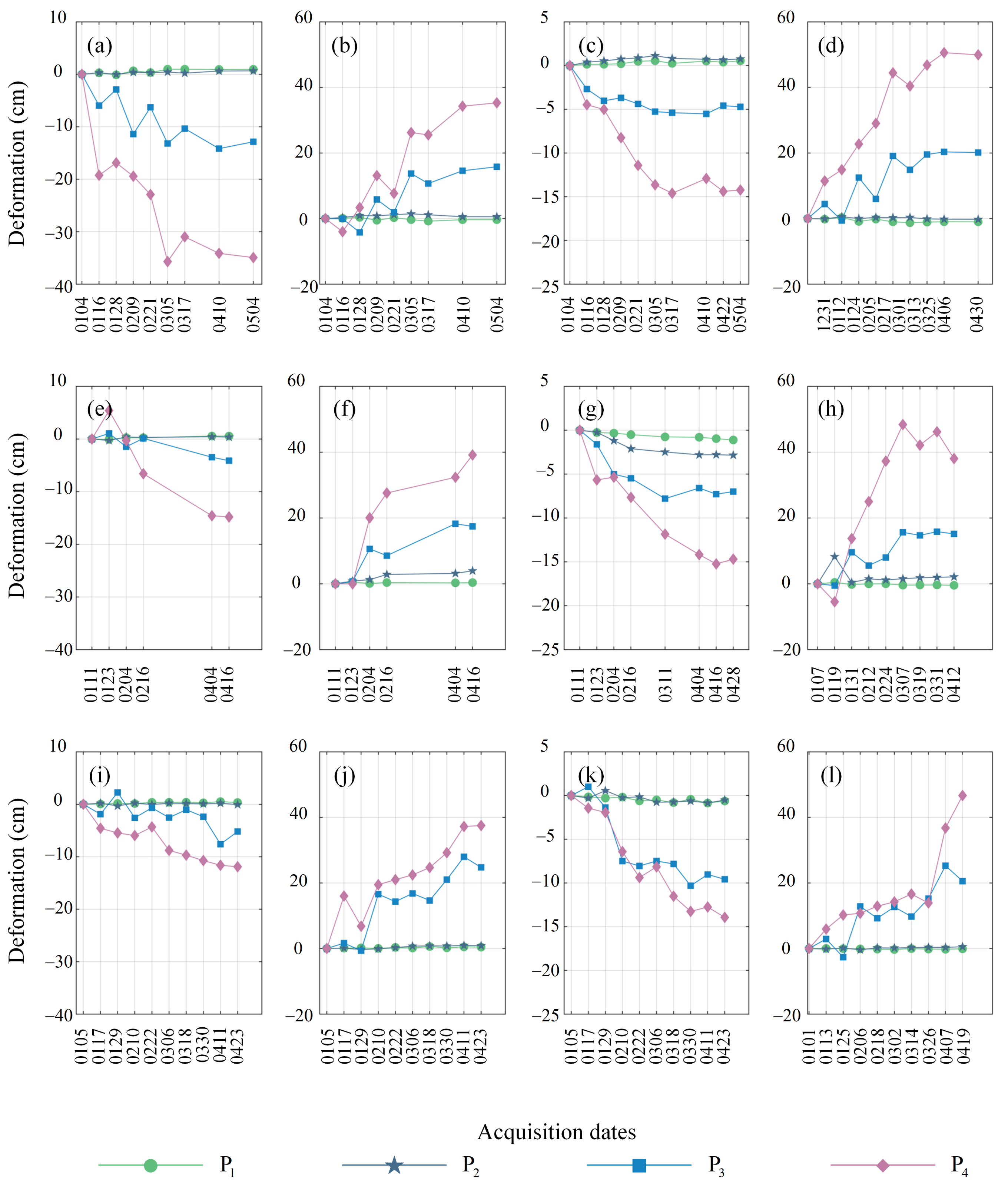
| Feature Points | Years (Movement Direction) | |||||
|---|---|---|---|---|---|---|
| 2019 (Vertical) | 2019 (Horizontal) | 2020 (Vertical) | 2020 (Horizontal) | 2021 (Vertical) | 2021 (Horizontal) | |
| P | −0.1 | 0.1 | 0.1 | 0.1 | 0 | 0 |
| P | −0.6 | 0.5 | −0.3 | 0.4 | −0.3 | 0.4 |
| P | −12.8 | 15.8 | −4.1 | 17.4 | −7.6 | 24.7 |
| P | −34.9 | 35.3 | −14.8 | 39.1 | −11.9 | 37.5 |
| Flight Direction | Year | ||
|---|---|---|---|
| 2019 | 2020 | 2021 | |
| Ascending | 0.85 | 0.67 | 0.75 |
| Descending | 0.68 | 0.71 | 0.81 |
| Deformation Results | LOS | 2D | ||
|---|---|---|---|---|
| Ascending | Descending | Vertical | Horizontal | |
| Study of Chen et al. | −13.6 | 16.7 | 9.4 | 21.7 |
| Results in the current work | −14.6 | 19.0 | 5.7 | 23.2 |
| Deformation difference | 1.0 | −2.3 | 2.7 | −1.5 |
Disclaimer/Publisher’s Note: The statements, opinions and data contained in all publications are solely those of the individual author(s) and contributor(s) and not of MDPI and/or the editor(s). MDPI and/or the editor(s) disclaim responsibility for any injury to people or property resulting from any ideas, methods, instructions or products referred to in the content. |
© 2023 by the authors. Licensee MDPI, Basel, Switzerland. This article is an open access article distributed under the terms and conditions of the Creative Commons Attribution (CC BY) license (https://creativecommons.org/licenses/by/4.0/).
Share and Cite
Zhu, Y.; Zhou, C.; Zhu, D.; Wang, T.; Zhang, T. Interannual Variation of Landfast Ice Using Ascending and Descending Sentinel-1 Images from 2019 to 2021: A Case Study of Cambridge Bay. Remote Sens. 2023, 15, 1296. https://doi.org/10.3390/rs15051296
Zhu Y, Zhou C, Zhu D, Wang T, Zhang T. Interannual Variation of Landfast Ice Using Ascending and Descending Sentinel-1 Images from 2019 to 2021: A Case Study of Cambridge Bay. Remote Sensing. 2023; 15(5):1296. https://doi.org/10.3390/rs15051296
Chicago/Turabian StyleZhu, Yikai, Chunxia Zhou, Dongyu Zhu, Tao Wang, and Tengfei Zhang. 2023. "Interannual Variation of Landfast Ice Using Ascending and Descending Sentinel-1 Images from 2019 to 2021: A Case Study of Cambridge Bay" Remote Sensing 15, no. 5: 1296. https://doi.org/10.3390/rs15051296