Clock Ensemble Algorithm Test in the Establishment of Space-Based Time Reference

Abstract

A new concept of a space-based synchronized reference network is proposed with the development of an optical frequency reference and laser inter-satellite link. To build such time reference, three clock ensemble algorithms, namely the natural Kalman timescale (NKT) algorithm, the reduced Kalman timescale (RKT) algorithm, and the two-stage Kalman timescale (TKT) algorithm are considered. This study analyzes and compares the performance of these algorithms using BDS, GPS, and Galileo satellite clock data from the GFZ GNSS clock corrections, which will be used in constructing future space-based time references. The study shows that the NKT algorithm improves frequency stability by 0.1–0.2 orders of magnitude in the short and medium term. When the satellite clock is mostly a hydrogen clock, the RKT and NKT are close, and the short and medium-term frequency stability slightly increases. In contrast, the TKT algorithm produces a timescale that improves frequency stability by 1–3 orders of magnitude. A quadratic polynomial model predicts the three timescales, with the results indicating that the short-term prediction accuracy of the satellite clock is within 1ns, and the TKT algorithm’s prediction accuracy is 1–2 orders of magnitude higher than that of the NKT and RKT algorithms. With the deployment of next-generation Low Earth Orbit (LEO) satellites equipped with higher-precision clocks, the space-based time reference system will achieve improved accuracy and greater potential for practical applications.

1. Introduction

Taking advantage of two rapidly developing technologies, e.g., optical frequency references and inter-satellite laser links [1,2], a new concept of establishing a network of space-based synchronized references has been widely discussed for future GNSS systems. For instance, a future Galileo-like medium earth orbit (MEO) constellation, Kepler, has been proposed by the German Aerospace Center (DLR), which could be characterized by both MEO and LEO segments and the innovative key features of optical inter-satellite links delivering highly precise range measurements and of optical frequency references enabling a perfect time synchronization within the complete constellation [3,4,5].

With the help of space-based time-synchronized references, GNSS can attain many benefits from the following aspects. Firstly, the broadcast of navigation signals could be synchronized to a level far superior to modern GNSSs. Secondly, a significant reduction or even the entire elimination of the satellite clock parameters could be achieved in the estimation process [3,6]. Thirdly, a better separation of uncertainties in the spatial and time domains could be obtained to enhance orbit determination. Moreover, a relativistic navigation system could be realized so that the satellite orbits are determined through the dissemination of each satellite’s proper time, and users estimate their own positions without the need to apply relativistic corrections. In addition, the synchronized signals also have potential impacts on the monitoring of the Earth’s gravity field, the provision of terrestrial reference frames, atmosphere sensing applications, and GNSS reflectometry [4].

In a space-based synchronized time reference, LEOs can be used as moving monitoring stations to achieve global tracking coverage of the MEOs. Thus, high-stability atomic clocks onboard and high precision time comparison between clocks is essential in the first place. Based on the time offsets of every individual clock, a proper composite clock algorithm is required to estimate a weighted average out of all ensemble clock readings, serving as the newly established system time. With the appropriate adjustment, the system time can keep coordinated with other standard time references similar to UTC or GNSS time. Finally, similar to the GNSS system, the space-based system time can provide users with ordinary time service and enable privileged users to build their time system by sharing detailed time comparison information.

When building the terrestrial time scale, the commonly used composite clock algorithms are the ALGOS algorithm (used by BIPM [7]) and the AT1 algorithm (used by the National Institute of Standards and Technology (NIST) [8]). Alternatively, the Kalman filter algorithm was developed in the 1980s [9,10], which allows for the addition or deletion of clocks at any time and provides automatic error detection and correction. With the continuous improvement of the algorithm, especially the reduction in the estimation error matrix [11,12] and the improvement of the medium and short-term frequency stability of the timescale [13], the Kalman filter algorithm has become mature and is widely used in GNSS to satisfy the real-time requirement [14].

What algorithm should be used for the space-based synchronized reference is still an important subject to be explored. In this work, we analyze the performance of three algorithms, namely the Natural Kalman clock ensemble algorithm (NKT) [15], the Reduced Kalman clock ensemble algorithm (RKT) [16], and the two-stage Kalman clock ensemble algorithm (TKT) [17], in establishing space-based time system in detail. In addition, simulation data have been used to compare and examine the timescale prediction accuracy of these three algorithms.

2. Clock Ensemble Algorithm

2.1. Infrastructure and System Architecture of Space-Based Time Reference

A space-based timescale hinges upon the manufacture and measurement of high-precision space atomic frequency standards (SAFS). As to the former aspect, besides three classical options: the thermal Cs beam, the hydrogen maser (H-maser) (passive or active), and the Rb atomic frequency standard (RAFS), there come several successors such as mercury trapped-ion [18,19], and some other Cs beam or Rb vapor cell clocks with new optical technologies [20,21,22,23,24]. The frequency stability of new generation clocks in both the short and long term is higher than that of classic satellite clocks in half or even one order of magnitude [1], and our approach to optical lattice clock, whose uncertainty is currently known as the least on the ground [25].

As to the latter aspect, the measurement and synchronization of the space-borne atomic clocks are carried out by orbit determination and time synchronization (ODTS) technologies. Though GPS, Galileo, and BDS use different ODTS strategies, the basic means are satellite-ground unidirectional and bidirectional time comparison techniques [26]. They can lead to orbit precision of 5–30 cm for MEO in most GNSSs [27]. According to the Multi-GNSS Experiment (MGEX) final products, the accuracy of satellite clock bias is about 0.3 ns for GPS and 0.6~1.2 ns for MEO in BDS [28,29]. Only using a satellite-ground link makes the estimated parameters, such as the radial direction of the orbit, the clock bias, and the antenna phase center offset, have strong degeneracy. Inter-satellite Link(ISL) can bring great profit to break this degeneracy and improve the precision of orbit and clock bias [30]. BDS began to test ISL in Ka-band in 2016 and applied ISL to BDS-3 to promote global service capability [31,32]. Thanks to ISL, the clock predicting error can be improved from 2~4 ns to less than 1 ns [33]. Compared to the precision of time comparison of the clock ensemble on the ground, there remains a certain disparity. To compare time over a long distance, two-way satellite time and frequency transfer (TWSTFT) and precise point positioning (PPP) are advised by BIPM [34,35,36]. The stability of time comparison using PPP and TWSTFT are 0.3 and 0.2 ns, respectively, and the accuracy with TWSTFT is 0.5~0.75 ns [35]. Optical fiber brings the highest accuracy of time and frequency transferring, which is better than 0.1 ns [37,38]. Since laser inter-satellite link leads to higher time comparison accuracy, it may push space-based timescale to catch up with ground-based timescale.

At present, the majority of LEO constellations are in the testing or basic setup stages. Some of them aim to provide stable and reliable broadband Internet communication services worldwide, and some of them aim to augment current GNSS. With high precision SAFS, it also has the potential to expand into a navigation constellation, and its capability to provide positioning, navigation, and timing services has been confirmed [39]. Especially high-quality GNSS products can obtain from IGS or its analysis centers, and high-accuracy services are provided by BDS and Galileo with B2b and E6-B signals, respectively [40,41,42]. LEO can achieve centimeter orbit precision by PPP technique with high accuracy carrier phase bias correction [40].

Based on all the technical progress mentioned above, the idea of establishing a space-based time system has been widely discussed. For instance, the Kepler system provides one possible architecture, that is, six LEOs adding to the Galileo-like system, where the LEOs serve as reference stations. With the continuous development of LEO satellite technology and the GNSS system, it is expected that more space-based time systems will be proposed in the future.

2.2. Natural Kalman Clock Ensemble Algorithm

Both the ALGOS algorithm and the AT1 algorithm mentioned above are weighted average algorithms, the keys of which are weight and predicted value. Different weights and predicted values will result in different algorithm performances and application scenarios. Different from the weighted average algorithm, the Kalman algorithm proposed by Barnes in 1982 focuses on estimation. The Kalman algorithm optimizes the variance between the reference clock and the ideal clock and takes the estimated value as the correction to generate the timescale [43,44].

The Kalman algorithm is based on a discrete and dynamic model of atomic clocks. The Kalman filter is constructed by superimposing all the single clock models in the clock group. The deviation between all clocks and reference clocks is the input, and the output is estimations of all clock phases, frequency, or frequency drift. The satellite clock data used in this paper are primarily hydrogen clocks and a few rubidium and cesium clocks. For hydrogen clocks, the Random-run frequency modulation noise (RRFM) is not obvious, and it is less affected by frequency drift [45,46]. According to this characteristic of the hydrogen clock, and a few rubidium clocks and cesium clocks have little influence on the result of the algorithm, this paper only considers phase and frequency in the Kalman filter, not frequency drift. A clock group contains N clocks. All conform to the following model

$$\left[\begin{array}{c}{x}_i\left(t\right)\\ y_i\left(t\right)\end{array}\right]=\left[\begin{array}{cc}1& T\\ 0& 1\end{array}\right]\left[\begin{array}{c}{x}_i\left(t-1\right)\\ y_i\left(t-1\right)\end{array}\right]+\left[\begin{array}{c}{\xi }_i\left(t\right)\\ {\eta }_i\left(t\right)\end{array}\right]$$

(1)

$$Q_i=\left[\begin{array}{cc}{E}_i& 0\\ 0& H_i\end{array}\right]$$

(2)

where $x_i\left(t\right)$ represents the time deviations of all the clocks; $y_i\left(t\right)$ is the frequency deviation; $T$ is the time interval; $Q_i$ is the system noise matrix; ${\xi }_i$ is white frequency modulation (WFM), and the variance is $E_i$; ${\eta }_i$ is the random walk frequency modulation (RWFM), and the variance is $H_i$.

According to the Kalman filtering model, the equation of the clock group is written

$$X\left(t\right)=\Phi X\left(t-1\right)+W\left(t\right)$$

(3)

$$Z\left(t\right)=HX\left(t\right)+V\left(t\right)$$

(4)

where

$$X\left(t\right)=\left[\begin{array}{c}\begin{array}{c}{x}_1\left(t\right)\\ y_1\left(t\right)\\ \begin{array}{c}{x}_2\left(t\right)\\ y_2\left(t\right)\\ ⋮\end{array}\end{array}\\ x_N\left(t\right)\\ y_N\left(t\right)\end{array}\right]$$

$$\Phi =\left[\begin{array}{ccc}\begin{array}{cc}1& T\\ 0& 1\end{array}& & \\ & \ddots & \\ & & \begin{array}{cc}1& T\\ 0& 1\end{array}\end{array}\right]$$

$$W\left(t\right)=\left[\begin{array}{c}\begin{array}{c}{\xi }_1\left(t\right)\\ {\eta }_1\left(t\right)\\ \begin{array}{c}{\xi }_2\left(t\right)\\ {\eta }_2\left(t\right)\\ ⋮\end{array}\end{array}\\ {\xi }_N\left(t\right)\\ {\eta }_N\left(t\right)\end{array}\right]$$

$$H=\left[\begin{array}{ccc}\begin{array}{ccc}1& 0& -1\\ 1& 0& 0\end{array}& \begin{array}{ccc}0& 0& 0\\ 0& -1& 0\end{array}& \begin{array}{ccc}\cdots & 0& 0\\ \cdots & 0& 0\end{array}\\ \begin{array}{ccc}⋮& ⋮& ⋮\\ 1& 0& 0\end{array}& \begin{array}{ccc}⋮& ⋮& ⋮\\ 0& 0& 0\end{array}& \begin{array}{ccc}⋮& ⋮& ⋮\\ \cdots & -1& 0\end{array}\end{array}\right]$$

$H$ is a matrix of ±ones and zeroes such that each row takes the difference of two-phase components of $X$. In Kalman filtering, every clock is identical. No matter which one is selected as the reference clock, it will not affect the final result. In practice, the reference clock may have missing observations. In the filtering process, the missing value is ignored since each clock is equivalent, we can choose other clocks with observed values as reference clocks, and then the processing continues. One convention in the $H$ matrix is to use the first clock as the reference clock. When there is a change in the reference clock, the position of “1” in the $H$ matrix must be adjusted accordingly.

The Kalman filter equations are described in the following

$$\left\{\begin{array}{l}{\widehat{X}}_{t,t-1}=\Phi X_{t-1,t-1}\\ P_{t,t-1}=\Phi P_{t-1,t-1}{\Phi }^{\prime }+Q\\ K=P_{t,t-1}H\prime {\left[H{P}_{t,t-1}{H}^{\prime }+R\right]}^{-1}\\ {\widehat{X}}_{t,t}={\widehat{X}}_{t,t-1}+K\left[Z\left(t\right)-H{\widehat{X}}_{t,t-1}\right]\\ P_{t,t}=(I-KH)P_{t,t-1}\end{array}\right.$$

(5)

where $P$ is the error variance matrix of $X$, $Q$ is the noise matrix, $K$ is the Kalman gain matrix, and $R$ is the measurement noise covariance matrix.

The value obtained by the Kalman filter is the time deviation between each clock and TA (Atomic time. In this paper, it refers to the ideal timescale generated by the algorithm.). Subtract this value from the time deviation of each clock to attain the “correction clock,” a total of N correction clocks. Any correction clock can be defined as a timescale generated by the algorithm. In fact, the value of a single timescale cannot be known, and what can be known is the time deviation between the two timescales. Therefore, TA is usually represented by the time deviation between it and the reference clock.

2.3. Reduced Kalman Clock Ensemble Algorithm

The generated timescales for the NKT algorithm tend to optimize the long-term stability of the corrected clocks, regardless of their short-term stability [47]. In Kalman filter estimation, the diagonal phase variance entries of the error covariance matrix $P$ grow without bound [48]. If the phase error variance element of $P$ is set to zero after each measurement without disturbing the desired output of the Kalman filter, the P matrix can be prevented from becoming out of control, thus giving a more stable calculation. This operation is called x-reduction [16].

$P$ is x-reduced, it is shown that

$$P_{ij}=\left[\begin{array}{cc}0& 0\\ 0& p(y_i,y_j)\end{array}\right]$$

The reduced Kalman timescale, which is designed to minimize the mean squared increments of the corrected clocks instead of their values at one time, produces good results for stability over all available averaging times [48].

2.4. Two-Stage Kalman Clock Ensemble Algorithm

The NKT algorithm mainly optimizes the long-term stability of the time scale but cannot effectively improve the short-term and medium stability. The TKT algorithm uses the characteristics of the atomic clock model to filter out WFM by one-stage filtering and improves the short and medium-term frequency stability of the time scale [49].

In the two-stage Kalman filter clock ensemble algorithm, the first filter is used to estimate the two statuses of the clock. There are WFM and RWFM in the first status and only RWFM in the second status. The second filter is similar to the natural Kalman filter, except that there is only one status vector, the phase. It is used to generate the timescale, and the input is the output of the first filter. In this way, the algorithm is equivalent to weighting the time series containing only RWFM. The generated timescale only contains RWFM, and the short and medium-term frequency stability is higher.

The principle is as follows.

In a clock group of $N$ clocks, the $i+1$ clock is subtracted from the first clock, and the resulting time deviation is denoted $Z_i\left(t\right)$, with a total of $N-1$ time deviation. Therefore, there are $N-1$ filters and $N-1$ time deviation processed, respectively. According to the atomic clock stochastic differential equation model shown below

$$\left\{\begin{array}{l}{X}_1\left(t\right)=x_0+y_0·t+1/2·d·t^2+{\sigma }_1·W_1\left(t\right)\\ +{\sigma }_2·{\int }_0^t{W}_2\left(s\right)ds\\ X_2\left(t\right)=y_0+d·t+{\sigma }_2·W_2\left(t\right)\end{array}\right.$$

(6)

$W_1\left(t\right)$ and $W_2\left(t\right),$ respectively, represent two independent Wiener processes, and each Wiener process follows a normal distribution whose mean is 0 and variance is time $t$. ${\sigma }_1$ and ${\sigma }_2$ are the diffusion coefficients of the two Wiener processes, respectively, which are used to indicate the intensity of noise. The integral of $W_1\left(t\right)$ and $W_2\left(t\right)$ against time $t$ is WFM and RWFM, respectively [50].

Attain two status estimators, denoted as ${\widehat{X}}_{1,i}(t)$ and ${\widehat{X}}_{2,i}(t)$. When the Kalman filter is used for status estimation, ${\widehat{X}}_{1,i}(t)$ contains WFM and RWFM, while ${\widehat{X}}_{2,i}(t)$ contains only RWFM.

Then, the time deviation is reconstructed, and for each estimate, let

$${\tilde{X}}_1\left(t+1\right)={\tilde{X}}_1\left(t\right)+{\widehat{X}}_2\left(t\right)·T$$

(7)

Taking the initial value of the ${\tilde{X}}_1\left(t\right)$ to be zero, Equation (7) can be rewritten as

$${\tilde{X}}_1\left(t\right)=\sum _{m=0}^{t-1}{\widehat{X}}_2\left(m\right)·T$$

(8)

Therefore, ${\tilde{X}}_1\left(t\right)$ is reconstructed through the estimator ${\widehat{X}}_2\left(t\right)$ to obtain the reconstructed time deviation. The WFM in the time deviation $Z\left(t\right)$ is filtered out by the first filter and the reconstruction of the time difference, and the reconstructed time deviation containing only RWFM is obtained. Finally, the second filter is a single-status Kalman filter, which is used to generate TA. Since each reconstructed clock only contains RWFM, TA only contains RWFM.

3. Experimental Analysis

In practice, both the ISL data and the satellite clock offsets data (calculated with PPP or ODTS technique) can be used for the establishment of a space-based timescale. Due to the serious discontinuity of the publicly available ISL data, here we adopt the MGEX satellite clock products to test the three clock ensemble algorithms mentioned in chapter 2. It is worth noting that the performance of the next-generation optical frequency standard will be better than the GNSS onboard clock. Therefore, the performance of all tested algorithms in future practical applications should be better than the analysis results in this paper.

3.1. Observed Data

Observed data used in this paper are GFZ GNSS clock corrections (deviations of the satellite clock with respect to the GPS time, download at ftp://ftp.gfz-potsdam.de/GNSS/products/mgex/, accessed on 10 June 2021), the start and end time are from 10 June 2021 to 10 October 2021, and the sampling interval is 300 s.

For measured data, the reading of a single clock cannot be known, and all that can be known is the time difference between two clocks. Therefore, we need to choose one clock as the reference and compare it with other clocks. TA is represented by the time deviation with the reference clock. In view of this, the specific time deviation of TA is still unknown. Therefore, this paper divides these data into four groups to generate four TAs and subtract them to eliminate the offsets caused by the unpredictability of a single clock.

In this experiment, 16 onboard clocks of BDS, GPS, and Galileo systems are included, which are grouped as follows:

Group A: C25–C28 satellite onboard clocks of Beidou-3, all of which are hydrogen clocks, take C28 as the reference clock and make the difference with other clocks to obtain three groups of time deviation, denoted as A1, A2, and A3;

Group B: C29, C30, C34, and C35 satellite onboard clocks of Beidou-3, all of which are hydrogen clocks, take C29 as the reference clock, and make the difference with other clocks to obtain three groups of time deviation, denoted as B1, B2, and B3;

Group C: G08, G15, G19, and G22 satellite onboard clocks of GPS, in which G08 is a cesium clock, and the others are rubidium clocks, take G19 as the reference clock and make the difference with other clocks to obtain three groups of time deviation, denoted as C1, C2, and C3;

Group D: E02, E05, E13, and E19 satellite onboard clocks of Galileo, in which E19 is a rubidium clock, and the others are hydrogen clocks, take E02 as the reference clock and make the difference with other clocks to obtain three groups of time deviation, denoted as D1, D2, and D3.

3.2. Accuracy Evaluation of Observation Data

There are many methods to characterize the frequency stability of atomic clocks. In this paper, Allan variance is used to describe frequency stability [51]. The overlapping Allan deviation of the four groups is shown in Figure 1. In the figure, the blue circle and green square are groups A and B, respectively, representing the frequency stability of the BDS. The pink triangle is group C, representing the frequency stability of the GPS. The red diamond is group D, representing the frequency stability of the Galileo system. The dotted line shows the overlapping Allan deviation of the time deviation for each group. The Allan deviation of each group with a sampling interval of 86,400 s is given in

Table 1. Allan deviation of each group. The average interval is 86,400 s.

Group	Time Deviation	Allan Deviation (τ = 1 Day)
A	A1	$7.9560{ \times 10}^{-15}$
	A2	$6.9398{ \times 10}^{-15}$
	A3	$7.1120{ \times 10}^{-15}$
B	B1	$1.1840{ \times 10}^{-14}$
	B2	$1.5846{ \times 10}^{-14}$
	B3	$1.2103{ \times 10}^{-14}$
C	C1	$6.6612{ \times 10}^{-14}$
	C2	$1.0659{ \times 10}^{-14}$
	C3	$1.1856{ \times 10}^{-14}$
D	D1	$6.0926{ \times 10}^{-15}$
	D2	$6.4042{ \times 10}^{-15}$
	D3	$6.9688{ \times 10}^{-15}$

.

In Figure 1 and Table 1, C1 is obtained from G19–G08, and G08 is a cesium clock. Its short-term frequency stability is the worst, but its long-term frequency stability is good. When the sampling interval is less than one day, it can be seen that the three times deviation in group D has the best frequency stability, followed by group A, group B, and group C. It can be seen that Galileo’s onboard clock is better than BDS, and BDS is better than GPS. In addition, when the average interval is 1000 s, except in group C, the frequency stability of satellite clocks is mainly around $4{ \times 10}^{-14}$ to $1{ \times 10}^{-13}$. When the average interval is 10,000 s, the frequency stability can reach about $2{ \times 10}^{-14}$ to $1{ \times 10}^{-13}$. The frequency stability of C2 and C3 in group C was close to that of the other groups, while C1 was around 2 × 10⁻¹³. When the average interval is 10,000 s, the frequency stability of other clocks basically reaches the minimum value except for C1, all of which are in the order of $1{ \times 10}^{-15}$. As the average time interval increases, the frequency stability of other satellite clocks progressively deteriorates, whereas the frequency stability of C1 continues to improve, reaching the level of $1{ \times 10}^{-15}$. As mentioned above, hydrogen clocks have good short-term stability, while cesium clocks have good long-term stability.

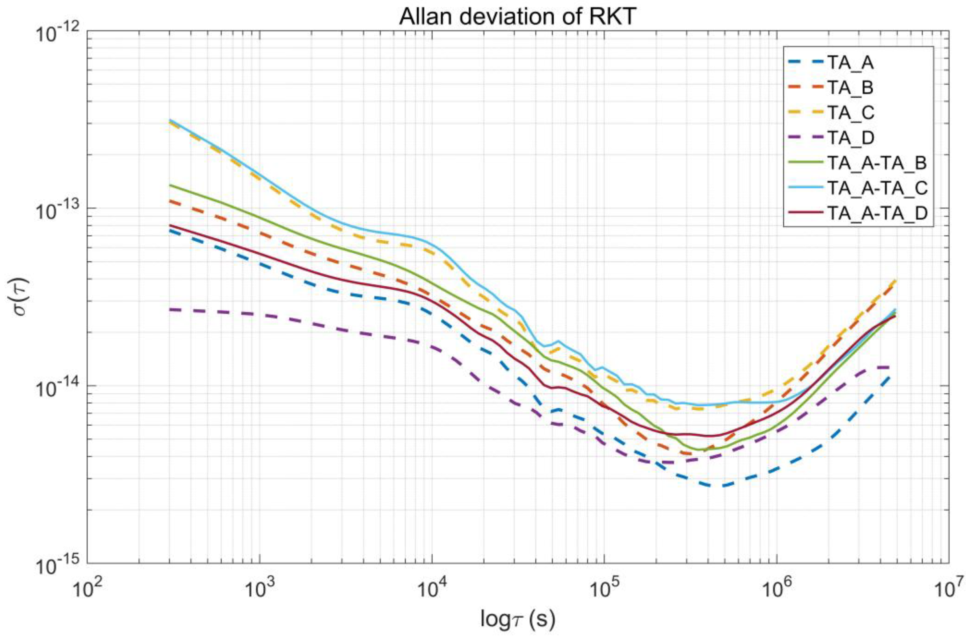
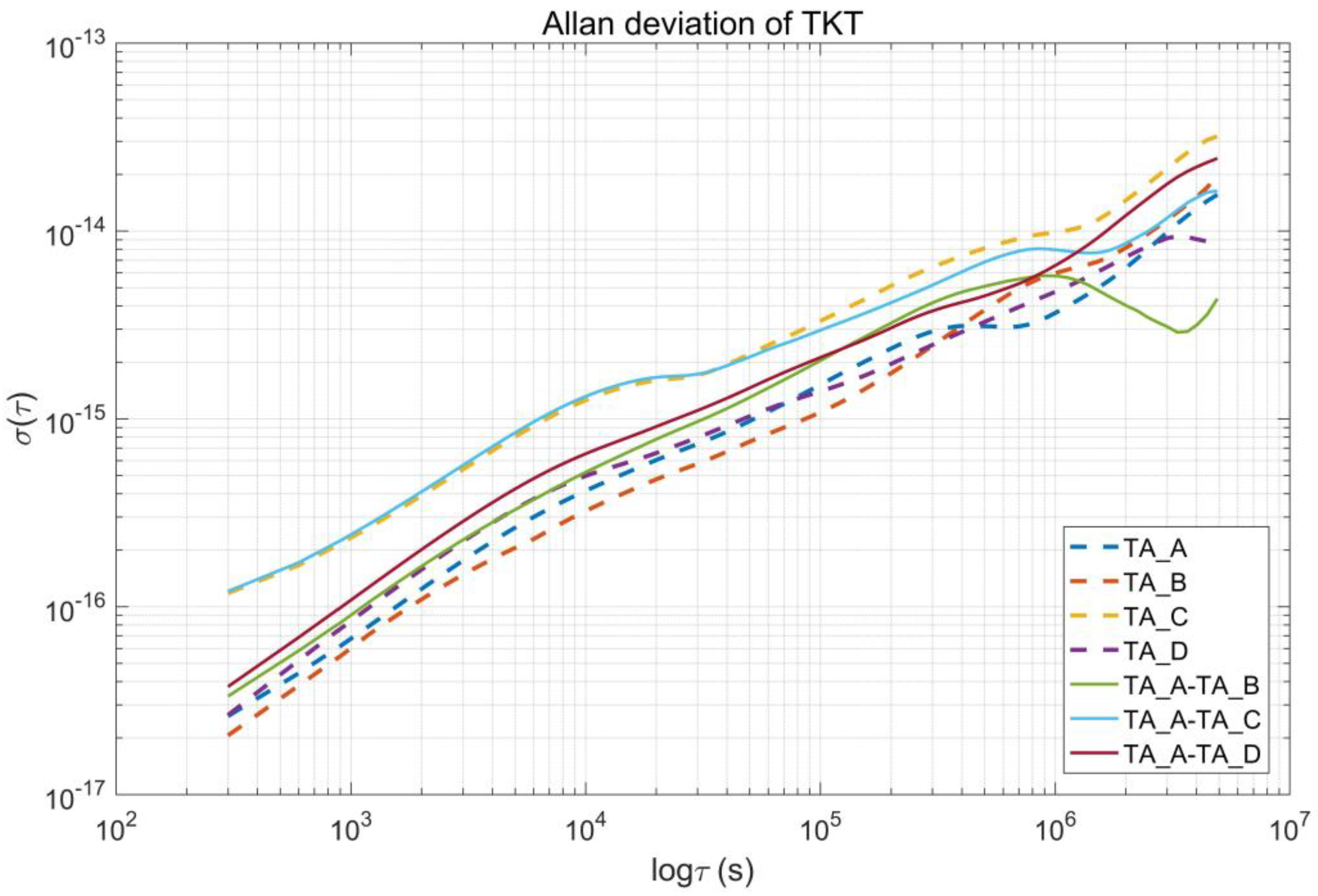
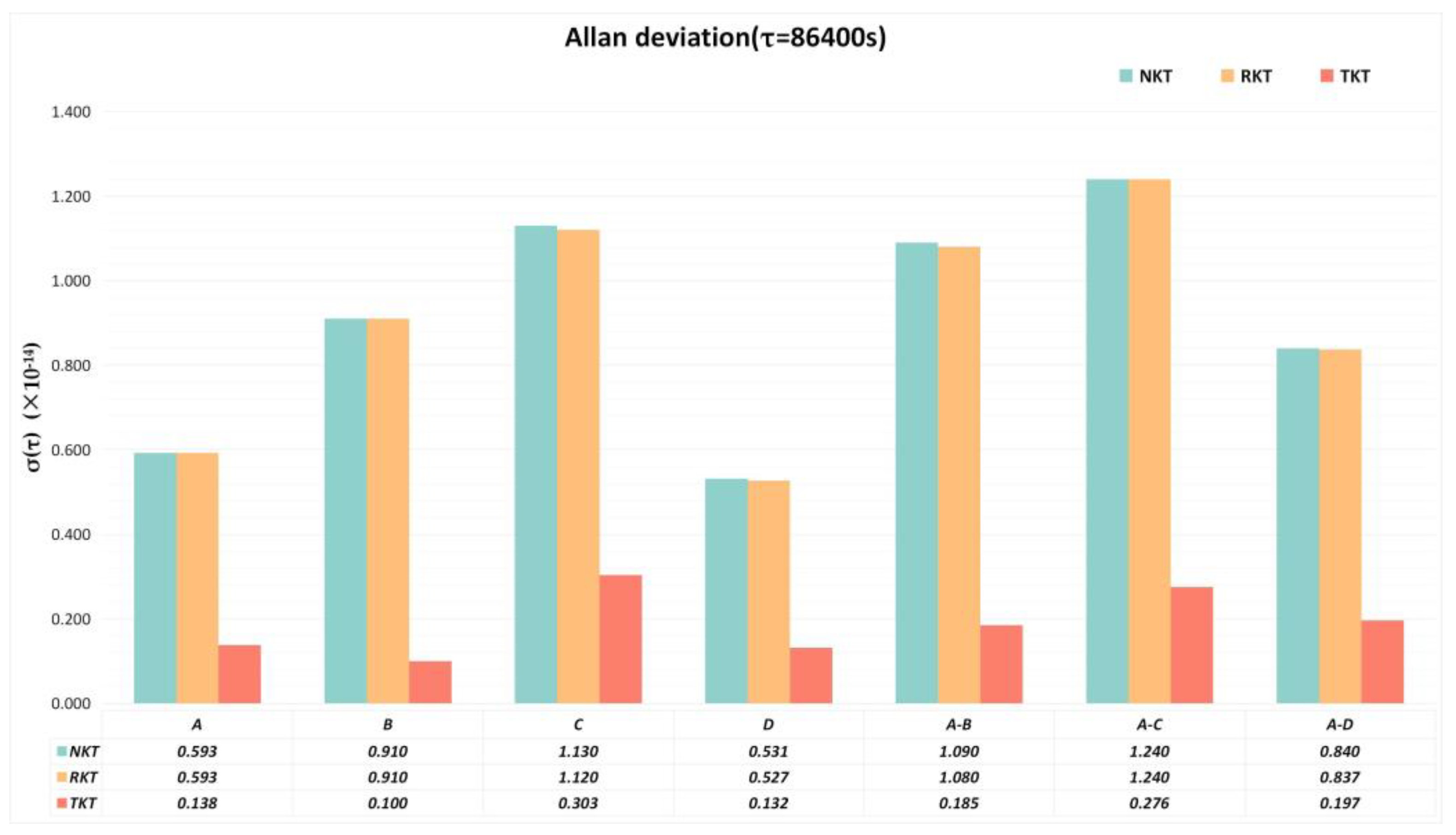
3.3. Frequency Stability of the Timescales Generated by the Three Algorithms

Unlike the simulation test, we cannot find the true value of TA to compare. Thus, the timescales of group A are subtracted from the other three groups to eliminate the offsets and analyze their frequency stability. For the NKT algorithm, the timescale is generated by three sets of time deviations in each group according to different weights. The weight is proportional to the inverse of the Allan deviation with a sampling interval of 86,400 s. The four timescales and their differences are shown in Figure 2. In the figure, the dotted line represents the four timescales, and the solid line represents the difference in the timescale. Allan deviation of 86,400 s sampling interval for each timescale and timescale difference is given in

Table 2. Allan deviation of each group (NKT). The average interval is 300 s and 86,400 s.

Time Series	Allan Deviation (τ = 300 s)	Allan Deviation (τ = 86,400 s)
TA_A	$7.88{ \times 10}^{-14}$	$5.93{ \times 10}^{-15}$
TA_B	$1.21{ \times 10}^{-13}$	$9.10{ \times 10}^{-15}$
TA_C	$3.87{ \times 10}^{-13}$	$1.13{ \times 10}^{-14}$
TA_D	$3.57{ \times 10}^{-14}$	$5.31{ \times 10}^{-15}$
TA_A-TA_B	$1.47{ \times 10}^{-13}$	$1.09{ \times 10}^{-14}$
TA_A-TA_C	$3.94{ \times 10}^{-13}$	$1.24{ \times 10}^{-14}$
TA_A-TA_D	$8.72{ \times 10}^{-14}$	$8.40{ \times 10}^{-15}$

.

Groups A and B are composed of BDS onboard clocks, group C is composed of GPS onboard clocks, and group D is composed of Galileo system onboard clocks. In Figure 2, TA_A-TA_B represents the frequency stability of the BDS timescale, which is $1.47{ \times 10}^{-13}$ at 300 s intervals and $1.09{ \times 10}^{-14}$ at 86,400 s intervals; TA_A-TA_C indicates the frequency stability of the GPS timescale, which is $3.94{ \times 10}^{-13}$ at 300 s intervals and $1.24{ \times 10}^{-14}$ at 86,400 s intervals; TA_A-TA_D indicates the frequency stability of the Galileo timescale, which is $8.72{ \times 10}^{-14}$ at 300 s intervals and $8.40{ \times 10}^{-15}$ at 86,400 s intervals. In the NKT algorithm, the short-term frequency stability of the Galileo system’s timescale is better than that of BDS, and BDS is slightly better than GPS. In addition, in the graph of Allan deviation, the part of the curve with slope −1 represents WFM, and the part with slope 1 represents RWFM. In Figure 2, we can see the obvious slopes of 1 and −1, indicating that the generated time scale still has WFM and RWFM.

For the RKT algorithm, x-reduction is performed in Kalman filtering and then obtains reduced timescale by calculating the weight of each group of clock deviation. The weights are also proportional to the inverse of the Allan deviation with a sampling interval of 86,400 s. The four timescales and their differences are shown in Figure 3, and Allan deviation of 86400s sampling interval for each timescale and timescale difference is given in

Table 3. Allan deviation of each group (RKT).

Time Series	Allan Deviation (τ = 300 s)	Allan Deviation (τ = 86,400 s)
TA_A	$7.50{ \times 10}^{-14}$	$5.93{ \times 10}^{-15}$
TA_B	$1.10{ \times 10}^{-13}$	$9.10{ \times 10}^{-15}$
TA_C	$3.06{ \times 10}^{-13}$	$1.12{ \times 10}^{-14}$
TA_D	$2.68{ \times 10}^{-14}$	$5.27{ \times 10}^{-15}$
TA_A-TA_B	$1.35{ \times 10}^{-13}$	$1.08{ \times 10}^{-14}$
TA_A-TA_C	$3.15{ \times 10}^{-13}$	$1.24{ \times 10}^{-14}$
TA_A-TA_D	$8.02{ \times 10}^{-14}$	$8.37{ \times 10}^{-15}$

.

In Figure 3, the reduced Kalman timescale contrasts little with the natural Kalman timescale. As shown in Table 3, for short-term (τ = 300 s) frequency stability, RKT has a small edge over NKT, with an increased range of about 0.01~0.1 orders of magnitude. For medium and long-term (τ = 86,400 s) frequency stability, the results of the two algorithms are nearly identical. This is because, for a clock set composed of clocks with good short-term stability and clocks with good long-term stability, the natural Kalman algorithm always tends to optimize the long-term stability without considering the short-term stability. The reduced Kalman algorithm, on the other hand, can synthesize the performance of clocks with varying performance to produce a result with greater stability over the entire sampling time range. However, in this experiment, the clock is primarily hydrogen clocks, and no clock with good short-term stability is available for optimization. As a result, when compared to the natural Kalman algorithm, the reduced Kalman algorithm only slightly improves short-term stability while having little effect on medium and long-term stability. In addition, as mentioned above, the obvious slopes of 1 and −1 can be seen in Figure 3, indicating that the generated timescales still have WFM and RWFM.

For the TKT algorithm, the four groups of time deviation need to be reconstructed using the first-stage filtering to obtain the reconstructed time deviation and then generate timescales according to different weights. The weights are also proportional to the inverse of the Allan deviation with a sampling interval of 86,400 s. The overlapping Allan deviation of the reconstructed time deviation is shown in Figure 4. The 86,400 s frequency stability of the reconstructed time deviation and the unreconstructed time deviation is given in Figure 5, and the values are shown in the table below. In the figure, blue represents the Allan deviation of the unreconstructed time deviation, and red represents the Allan deviation of the reconstructed time deviation. The sampling interval is 86,400 s. It can be seen that the short-term frequency stability of the reconstructed time deviation has been greatly improved, and the Allan deviation with a sampling interval of 86,400 s is improved by 0.1 to 1 order of magnitude.

The timescale generated by the TKT algorithm is shown in Figure 6. In the figure, the dotted line represents the four timescales, and the solid line represents the difference in the timescale. Allan deviation of 86,400 s sampling interval for each timescale and timescale difference is given in Figure 7.

In Figure 6 and Figure 7, the frequency stability of the timescale generated by the TKT algorithm is greatly improved, which is about 0.5~1 orders of magnitude higher than that of the NKT algorithm and RKT algorithm. The timescale frequency stability generated by the Galileo system and the BDS onboard clock is similar, which is slightly better than GPS. Meanwhile, the curve in Figure 6 has only the part with slope −1, and the part with slope 1 disappears and becomes a continuation of the part with slope −1. This means that the generated time scale is only RWFM, without WFM. This is consistent with the algorithm introduction in Section 2.4.

In addition, for the current three kinds of onboard clocks, no matter which clock ensemble algorithm is chosen, as expected, the hydrogen clock is more stable than the rubidium clock, and the rubidium clock is more stable than the cesium clock. Therefore, hydrogen clocks are a better choice when higher frequency stability is needed to establish space-based time references.

The frequency stability of the timescale is an approach to the value of commonly used timescales on the ground [52,53].

For the NKT algorithm, the generated timescale fully considers the short-term stability performance of each satellite clock. The clock with better short-term stability will have more weight. For all three systems, Galileo’s satellite clock is more stable in the short term, and the resulting timescale is more stable.

For the RKT algorithm, as mentioned above, since this experiment is primarily a hydrogen clock, there is no clock with better short-term stability to produce better short-term stability for the generated timescale. The result is nearly identical to that of the NKT algorithm.

For the TKT algorithm, because the first-stage filtering filters out high-frequency noise, the weight of each clock is determined by its long-term stability. Considering that the stability of hydrogen clocks is higher than rubidium clocks. Therefore, for the three systems, the satellite clocks of the BDS and Galileo systems are mainly composed of hydrogen masers, the stability of the generated timescales is similar, and they are all better than the GPS, mainly composed of rubidium clocks.

4. Satellite Clock Bias Prediction

The timescale is expressed as the bias of the satellite clock phase and the timescale itself. The prediction of the clock bias is often used in real-time scenarios. Thus, we tested the prediction accuracy of the three kinds of timescale generated by the NKT, the RKT, and the TKT algorithms as their evaluation criteria.

4.1. Prediction Models

Many prediction models of clock deviation have been developed with similar accuracy, e.g., the quadratic polynomial model, the gray model, and the Kalman filter model. Their accuracy is of a similar magnitude, and the quadratic polynomial model shows to be simpler in the calculation, more stable in practice, and more accurate in short-term prediction [54]. For the above reasons, we select this model to predict clock bias in our subsequent analysis.

The quadratic polynomial model fits the phase, frequency, and frequency drift parameters according to the physical characteristics of the satellite clock, and the fitting expression is as follows [55]:

$$y\left(t\right)=a_0+a_1\left(t_i-t_0\right)+a_2{\left(t_i-t_0\right)}^2+{∆}_i$$

(9)

where $y\left(t\right)$ is the clock observation, $a_0,a_1,a_2$ are three parameters of the satellite clock model, phase, frequency, and frequency drift, $t_0$ is the reference epoch of the satellite clock model, $t_i$ denotes the observation epoch. ${∆}_i$ is the residual of the prediction model.

As the most commonly used prediction model, the quadratic polynomial model is suitable for the rubidium atomic frequency standard, while for hydrogen and cesium frequency standards, the first-order polynomial model is a more appropriate choice. As a result, we use the first-order polynomial model for hydrogen and cesium clocks and the quadratic polynomial model for rubidium clocks.

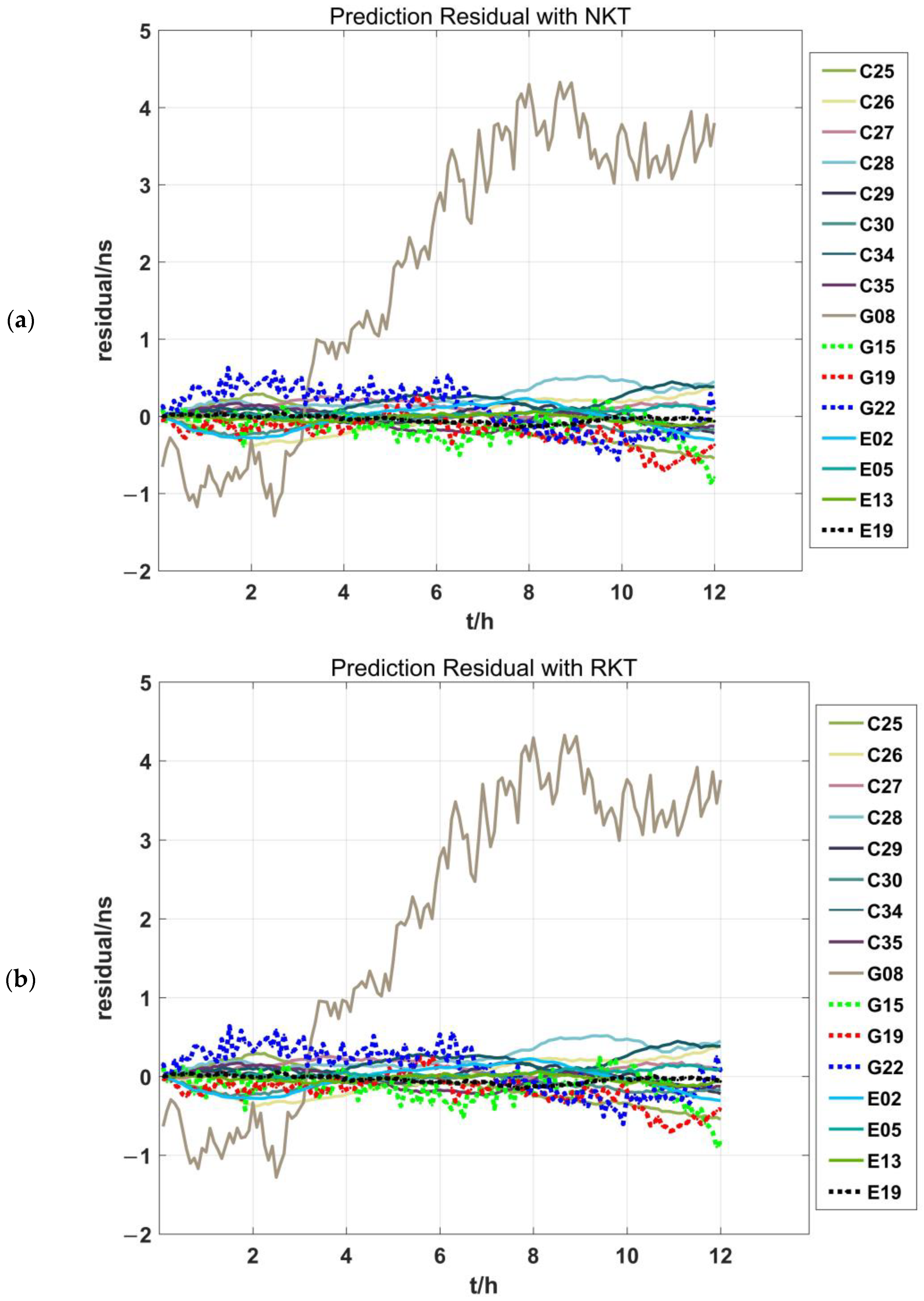
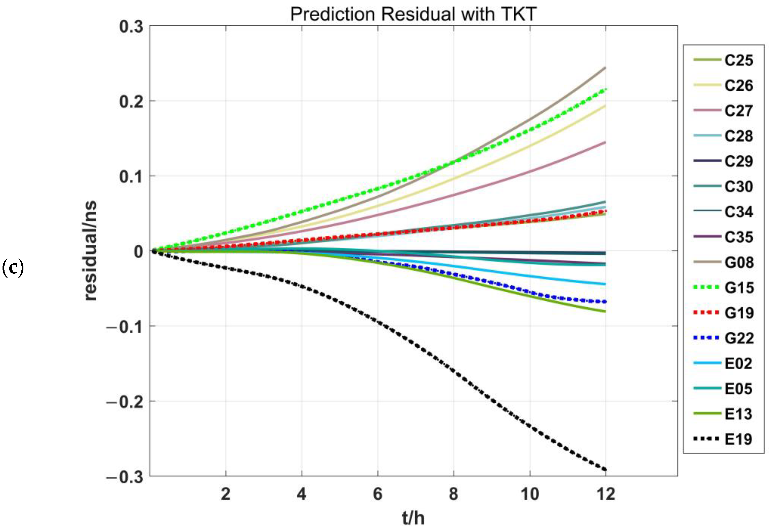
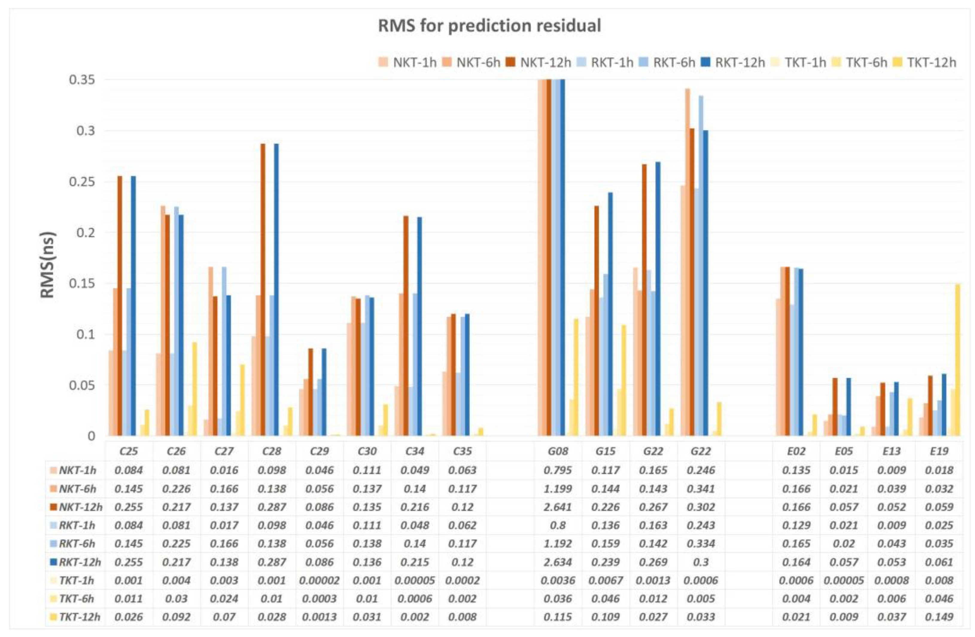
4.2. Satellite Clock Bias Prediction

In this paper, we fit the clock bias data sets, i.e., the bias between the satellite clock phase and the timescale, every hour with a moving window in the length of 12 h, and predict for the next 12 h at every fitting. The clock bias in the prediction arc is treated as a true value. We calculate the residual root mean square (RMS) to evaluate the prediction accuracy. The clock bias calculated with three clock ensemble algorithms is analyzed.

Take time clock data from 10 June 2021 as an example. Figure 8 displays the deviations in residuals between each satellite’s prediction results and the true values. The solid line in the figure represents the hydrogen clock and the cesium clock, which are fitted by a first-order polynomial model. The dotted line represents the rubidium clock, which is fitted by a quadratic polynomial model.

The prediction residual, shown in Figure 8, with durations ranging from 1 h to 12 h of the NKT algorithm and RKT algorithm, is within 0.4 ns~1 ns, and the general trend is rather consistent. The prediction residual of the TKT algorithm increases linearly from 0.01 ns to 0.3 ns. In terms of orders of magnitude, the prediction accuracy of the TKT algorithm is about 1–2 orders of magnitude higher than that of the NKT algorithm and RKT algorithm, and the shorter the prediction duration, the greater the difference in the prediction accuracy.

To focus on the different prediction periods, we calculated the RMS of the prediction residuals of each satellite clock of three timescales with 1, 6, and 12 h and depicted their statistical results in Figure 9. In the histogram, from left to right, each cluster represents the RMS of 1, 6, and 12 h prediction residuals of the NKT algorithm, RKT algorithm, and TKT algorithm, respectively. The specific values are listed in the table below the figure. To make the TKT prediction result distinguishable, the figure adapts the upper limit of the y-axis to fit the magnitude of other satellite clocks, which makes the RMS of G08 not fully exhibited.

The RMS of the prediction residual of the NKT algorithm is very close to that of the RKT algorithm, both of which are much larger than that of the TKT algorithm, no matter how long the prediction duration is. For the 16 satellites, the RMS of the prediction residual of the Galileo system is smaller than that of the BDS, and the BDS is smaller than that of the GPS. To generate a timescale, the satellite clock we used in GPS is a rubidium clock, which leads to inferior accuracy and stability to the hydrogen clock. This makes it intelligible why the prediction accuracy of the timescale generated with GPS satellite clocks is the worst. Yet it cannot explain the disparity between Galileo and BDS. Since they both employ hydrogen maser frequency standards that are approximate in accuracy and stability, there must be other factors polluting the satellite clock bias data. The clock bias series of GFZ is calculated with the methods of orbit determination and time synchronization (ODTS). As one of the estimated parameters, the clock bias has strong correlations with other parameters, such as orbit elements. Thus, the estimated error of clock bias not only comes from the measurement noise of the clock bias itself but also blends with the orbit error. It implies that the orbital dynamics modeling error for the Galileo system is smaller than that of BDS. Although both systems consist mainly of hydrogen clocks, Galileo’s prediction accuracy is still better than BDS’s.

In addition, we compared the RMS of the residual of the three algorithms. With the extension of the prediction duration, the RMS of the prediction residual of the NKT algorithm and RKT algorithm will raise, but the growth trend is relatively slow and occasionally will decrease. The RMS of the TKT algorithm will also increase, and the growth trend is conspicuous with a large range. This is consistent with the result shown in Figure 8. It is implicit that the prediction accuracy of the TKT algorithm has strong relevance with time, while that of the NKT algorithm and RKT algorithm remains rather stable. If the prediction period is one day or longer, the prediction residual of the TKT algorithm will gradually be larger than that of the other two algorithms, and the prediction accuracy will become worse. Thus, the timescale generated by the TKT algorithm is not recommended in the use of prediction longer than one day.

TKT can effectively suppress timescale low-frequency noise, and this advantage can benefit users. According to our comparison of the prediction results, for the prediction of a single frequency reference, the TKT prediction results are higher than the NKT and RKT. It indicates that the TKT algorithm reduces the influence of low-frequency noise of other frequency standards on the modeling of this frequency standard. Therefore, when users use the satellite clock difference model based on this scale to correct their ranging, they only receive low-frequency errors of a single satellite clock and eliminate the pollution of low-frequency errors of other satellites.

5. Conclusions

The LEO constellation provides several advantages in satellite navigation, such as strong signals on the ground and rapidly changing geometric positions. These benefits complement other GNSS constellations, such as MEO and HEO, and enhance the accuracy, integrity, continuity, and availability of GNSS. As a result, the LEO constellation has become a research focus in the satellite navigation field.

This paper presents a novel concept of establishing a network of space-based synchronized references for time synchronization. We discuss the infrastructure and system architecture needed to establish the time reference, taking advantage of the development of optical frequency reference and inter-satellite laser link technology. The study evaluates the performance of three Kalman clock ensemble algorithms, the natural Kalman clock ensemble algorithm, the reduced Kalman clock ensemble algorithm, and the two-stage Kalman clock ensemble algorithm, using the GFZ GNSS clock corrections. The results show that the accuracy of NKT and RKT are close when the satellite clock type is the same, although TKT has higher short and medium-term stability. Given the need for higher stability on timescales, hydrogen clocks outperform rubidium and cesium clocks for onboard satellites. Furthermore, a polynomial model is applied to predict the timescale generated by each algorithm. For prediction durations of less than one day, the TKT algorithm exhibits prediction residuals that are 1–2 orders of magnitude lower than those of NKT and RKT algorithms. Finally, the prediction accuracy of Galileo is found to be superior to that of BDS, while BDS is superior to GPS.

Subsequently, our goal is to acquire clock data from LEO satellites and integrate them with data from medium and high-orbit satellite clocks to produce space-based time references. This approach will result in a more stable timescale that can be employed in a wider array of circumstances.

References

1. Batori, E.; Almat, N.; Affolderbach, C.; Mileti, G. GNSS-grade space atomic frequency standards: Current status and ongoing developments. Adv. Space Res. 2021, 68, 4723–4733. [Google Scholar] [CrossRef]
2. Michalak, G.; Glaser, S.; Neumayer, K.H.; Konig, R. Precise orbit and Earth parameter determination supported by LEO satellites, inter-satellite links and synchronized clocks of a future GNSS. Adv. Space Res. 2021, 68, 4753–4782. [Google Scholar] [CrossRef]
3. Giorgi, G.; Schmidt, T.D.; Trainotti, C.; Mata-Calvo, R.; Fuchs, C.; Hoque, M.M.; Berdermann, J.; Furthner, J.; Gunther, C.; Schuldt, T.; et al. Advanced technologies for satellite navigation and geodesy. Adv. Space Res. 2019, 64, 1256–1273. [Google Scholar] [CrossRef]
4. Giorgi, G.; Kroese, B.; Michalak, G. Future GNSS constellations with optical inter-satellite links. Preliminary space segment analyses. In Proceedings of the IEEE Aerospace Conference, Big Sky, MT, USA, 2–9 March 2019. [Google Scholar]
5. Glaser, S.; Michalak, G.; Mannel, B.; Konig, R.; Neumayer, K.H.; Schuh, H. Reference system origin and scale realization within the future GNSS constellation “Kepler”. J. Geod. 2020, 94, 13. [Google Scholar] [CrossRef]
6. Gunther, C.; Inst, N. Kepler—Satellite Navigation without Clocks and Ground Infrastructure. In Proceedings of the 31st International Technical Meeting of the Satellite-Division-of-The-Institute-of-Navigation (ION GNSS), Miami, FL, USA, 24–28 September 2018; pp. 849–856. [Google Scholar]
7. Panfilo, G.; Arias, E.F. Algorithms for International Atomic Time. IEEE Trans. Ultrason. Ferroelectr. Freq. Control 2010, 57, 140–150. [Google Scholar] [CrossRef]
8. Parker, T.E.; Levine, J. Impact of new high stability frequency standards on the performance of the NIST AT1 time scale. IEEE Trans. Ultrason. Ferroelectr. Freq. Control 1997, 44, 1239–1244. [Google Scholar] [CrossRef] [Green Version]
9. Jones, R.H.; Tryon, P.V. Estimating Time from Atomic Clocks. J. Res. Natl. Bur. Stand. 1983, 88, 17–24. [Google Scholar] [CrossRef]
10. Weiss, M.A.; Allan, D.W.; Peppler, T.K. A Study of the NBS Time Scale Algorithm. IEEE Trans. Instrum. Meas. 1989, 38, 631–635. [Google Scholar] [CrossRef] [Green Version]
11. Panfilo, G.; Harmegnies, A.; Tisserand, L. A new weighting procedure for UTC. Metrologia 2014, 51, 285–292. [Google Scholar] [CrossRef]
12. Tavella, P. Statistical and mathematical tools for atomic clocks. Metrologia 2008, 45, S183–S192. [Google Scholar] [CrossRef]
13. Zucca, C.; Tavella, P. The clock model and its relationship with the allan and related variances. IEEE Trans. Ultrason. Ferroelectr. Freq. Control 2005, 52, 289–296. [Google Scholar] [CrossRef]
14. Schmidt, T.D.; Trainotti, C.; Isoard, J.; Giorgi, G.; Furthner, J.; Gunther, C.; Inst, N. Composite Clock Algorithms for System Time in Global Navigation Satellite Systems. In Proceedings of the 31st International Technical Meeting of the Satellite-Division-of-The-Institute-of-Navigation (ION GNSS), Miami, FL, USA, 24–28 September 2018; pp. 963–967. [Google Scholar]
15. Brown, K.R. The Theory of the GPS Composite Clock. Ionics 1991, 4, 223–242. [Google Scholar]
16. Greenhall, C.A. Forming stable timescales from the Jones-Tryon Kalman filter. Metrologia 2003, 40, S335–S341. [Google Scholar] [CrossRef]
17. Keller, J.Y.; Darouach, M. Optimal two-stage Kalman filter in the presence of random bias. Automatica 1997, 33, 1745–1748. [Google Scholar] [CrossRef]
18. Ren, W.; Li, T.; Qu, Q.Z.; Wang, B.; Li, L.; Lu, D.S.; Chen, W.B.; Liu, L. Development of a space cold atom clock. Natl. Sci. Rev. 2020, 7, 1828–1836. [Google Scholar] [CrossRef]
19. Burt, E.A.; Yi, L.; Tucker, B.; Hamell, R.; Tjoelker, R.L. JPL Ultrastable Trapped Ion Atomic Frequency Standards. IEEE Trans. Ultrason. Ferroelectr. Freq. Control 2016, 63, 1013–1021. [Google Scholar] [CrossRef]
20. Gharavipour, M.; Affolderbach, C.; Kang, S.; Bandi, T.N.; Gruet, F.; Pellaton, M.; Mileti, G. High performance vapour-cell frequency standards. J. Phys. Conf. Ser. 2016, 723, 012006. [Google Scholar] [CrossRef]
21. Arpesi, P.; Belfi, J.; Gioia, M.; Marzoli, N.; Romani, R.; Sapia, A.; Gozzelino, M.; Calosso, C.; Levi, F.; Micalizio, S.; et al. Rubidium Pulsed Optically Pumped Clock for Space Industry. In Proceedings of the Joint Conference of the IEEE International Frequency Control Symposium/Conference of the European-Frequency-and-Time-Forum (EFTF/IFC), Orlando, FL, USA, 14–18 April 2019. [Google Scholar]
22. Micalizio, S.; Calosso, C.E.; Levi, F.; Gozzelino, M.; Gioia, M.; Arpesi, P.; Sapia, A.; Romani, R.; Belfi, J.; Marzoli, N.; et al. Preliminary characterization of a Rb Pulsed Optically Pumped clock for space applications. In Proceedings of the IEEE International Workshop on Metrology for AeroSpace (MetroAeroSpace), Torino, Italy, 19–21 June 2019; pp. 682–686. [Google Scholar]
23. Kitching, J. Chip-scale atomic devices. Appl. Phys. Rev. 2018, 5, 38. [Google Scholar] [CrossRef]
24. Vanier, J.; Tomescu, C. The Quantum Physics of Atomic Frequency Standards: Recent Developments; CRC Press: Boca Raton, FL, USA, 2015. [Google Scholar]
25. Koller, S.B.; Grotti, J.; Vogt, S.; Al-Masoudi, A.; Dorscher, S.; Hafner, S.; Sterr, U.; Lisdat, C. Transportable Optical Lattice Clock with 7 x 10(-17) Uncertainty. Phys. Rev. Lett. 2017, 118, 6. [Google Scholar] [CrossRef] [Green Version]
26. Zhou, S.; Hu, X.; Liu, L.; He, F.; Tang, C.; Pang, J. Status of Satellite Orbit Determination and Time Synchronization Technology for Global Navigation Satellites System. Acta Astron. Sin. 2019, 60, 32. [Google Scholar]
27. Montenbruck, O.; Steigenberger, P.; Prange, L.; Deng, Z.G.; Zhao, Q.L.; Perosanz, F.; Romero, I.; Noll, C.; Sturze, A.; Weber, G.; et al. The Multi-GNSS Experiment (MGEX) of the International GNSS Service (IGS)—Achievements, prospects and challenges. Adv. Space Res. 2017, 59, 1671–1697. [Google Scholar] [CrossRef]
28. Uhlemann, M.; Gendt, G.; Ramatschi, M.; Deng, Z.G. GFZ Global Multi-GNSS Network and Data Processing Results. In Proceedings of the Scientific Assembly of the International-Association-of-Geodesy (IAG), Potsdam, Germany, 1–6 September 2013; pp. 673–679. [Google Scholar]
29. Yang, Y.; Yang, Y.; Wang, W.; Zhao, A. Accuracy Assessment for IGS MGEX Clock Products. J. Geomat. Sci. Technol. 2018, 35, 441–445. [Google Scholar]
30. Fernandez, F.A. Inter-satellite ranging and inter-satellite communication links for enhancing GNSS satellite broadcast navigation data. Adv. Space Res. 2011, 47, 786–801. [Google Scholar] [CrossRef]
31. Chen, J.; Hu, X.; Tang, C.; Zhou, S.; Guo, R.; Pan, J.; Li, R.; Zhu, L. Orbit determination and time synchronization for new-generation Beidou satellites: Preliminary results. Sci. Sin. Phys. Mech. Astron. 2016, 46, 85–95. [Google Scholar]
32. Tang, C.P.; Hu, X.G.; Zhou, S.S.; Liu, L.; Pan, J.Y.; Chen, L.C.; Guo, R.; Zhu, L.F.; Hu, G.M.; Li, X.J.; et al. Initial results of centralized autonomous orbit determination of the new-generation BDS satellites with inter-satellite link measurements. J. Geod. 2018, 92, 1155–1169. [Google Scholar] [CrossRef]
33. Pan, J.; Hu, X.; Tang, C.; Zhou, S.; Li, R.; Zhu, L.; Tang, G.; Hu, G.; Chang, Z.; Wu, S.; et al. System error calibration for time division multiple access inter-satellite payload of new-generation Beidou satellites. Chin. Sci. Bull. 2017, 62, 2671–2679. [Google Scholar] [CrossRef] [Green Version]
34. Arias, F.; Jiang, Z.; Lewandowski, W.; Petit, G. BIPM comparison of time transfer techniques. In Proceedings of the IEEE International Frequency Control Symposium and Exposition, Vancouver, BC, Canada, 29–31 August 2005; pp. 312–315. [Google Scholar]
35. Jiang, Z.; Lewandowski, W.W.; Konaté, H. TWSTFT Data Treatment for UTC Time Transfer. In Proceedings of the 41st Annual Precise Time and Time Interval Systems and Applications Meeting, Santa Ana Pueblo, New Mexico, 16–19 November 2009. [Google Scholar]
36. Petit, G.; Meynadier, F.; Harmegnies, A.; Parra, C. Continuous IPPP links for UTC. Metrologia 2022, 59, 14. [Google Scholar] [CrossRef]
37. Bauch, A.; Achkar, J.; Bize, S.; Calonico, D.; Dach, R.; Hlavac, R.; Lorini, L.; Parker, T.; Petit, G.; Piester, D.; et al. Comparison between frequency standards in Europe and the USA at the 10(-15) uncertainty level. Metrologia 2006, 43, 109–120. [Google Scholar] [CrossRef] [Green Version]
38. Xue, W.X.; Zhao, W.Y.; Quan, H.L.; Xing, Y.; Zhang, S.G. Cascaded Microwave Frequency Transfer over 300-km Fiber Link with Instability at the 10(-18) Level. Remote Sens. 2021, 13, 2182. [Google Scholar] [CrossRef]
39. Kassas, Z.M. Navigation from Low-Earth Orbit. In Position, Navigation, and Timing Technologies in the 21st Century; Wiley: Hoboken, NJ, USA, 2020; pp. 1381–1412. [Google Scholar]
40. Hauschild, A.; Montenbruck, O.; Steigenberger, P.; Martini, I.; Fernandez-Hernandez, I. Orbit determination of sentinel-6A using the galileo high accuracy service test signal. GPS Solut. 2022, 26, 13. [Google Scholar] [CrossRef]
41. Arnold, D.; Schaer, S.; Villiger, A.; Dach, R.; Jäggi, A. Undifference ambiguity resolution for GPS-based precise orbit determination of low Earth orbiters using the new CODE clock and phase bias products. In Proceedings of the International GNSS Service Workshop 2018, Wuhan, China, 29 October–2 November 2018. [Google Scholar]
42. Tang, C.P.; Hu, X.G.; Chen, J.P.; Liu, L.; Zhou, S.S.; Guo, R.; Li, X.J.; He, F.; Liu, J.H.; Yang, J.H. Orbit determination, clock estimation and performance evaluation of BDS-3 PPP-B2b service. J. Geod. 2022, 96, 17. [Google Scholar] [CrossRef]
43. Barnes, J.A.; Chi, A.R.; Cutler, L.S.; Healey, D.J.; Leeson, D.B.; McGunigal, T.E.; Mullen, J.A.; Smith, W.L.; Sydnor, R.L.; Vessot, R.F.C.; et al. Characterization of Frequency Stability. IEEE Trans. Instrum. Meas. 1971, IM20, 105–120. [Google Scholar] [CrossRef] [Green Version]
44. Barnes, J.A.; Allan, D.W.; Jones, R.H.; Tryon, P.V. Stochastic models for atomic clocks. In Proceedings of the 14th Annual Precise Time and Time Interval Systems and Applications Meeting, Greenbelt, MD, USA, 30 November 1982. [Google Scholar]
45. Wu, Z.Q.; Zhou, S.S.; Hu, X.G.; Liu, L.; Shuai, T.; Xie, Y.H.; Tang, C.P.; Pan, J.Y.; Zhu, L.F.; Chang, Z.Q. Performance of the BDS3 experimental satellite passive hydrogen maser. GPS Solut. 2018, 22, 13. [Google Scholar] [CrossRef]
46. Xu, Y.; Zeng, A.; Mu, Y. Performance Evaluation and Analysis of Beidou-3 On-orbit Atomic Clock. In China Satellite Navigation Conference (CSNC) 2020 Proceedings; Springer Singapore: Singapore, 2020; Volume 3, pp. 196–209. [Google Scholar]
47. Weiss, M.; Weissert, T. AT2, A New Time Scale Algorithm—AT1 Plus Frequency Variance. Metrologia 1991, 28, 65–74. [Google Scholar] [CrossRef] [Green Version]
48. Greenhall, C.A. A Review of Reduced Kalman Filters for Clock Ensembles. IEEE Trans. Ultrason. Ferroelectr. Freq. Control 2012, 59, 491–496. [Google Scholar] [CrossRef]
49. Wu, Y.; Gong, H.; Zhu, X.; Liu, W.; Ou, G. Twice Atomic Clock Steering Algorithm and Its Application in Forming a GNSS Time Reference. Acta Electron. Sin. 2016, 44, 1742–1750. [Google Scholar]
50. Galleani, L.; Sacerdote, L.; Tavella, P.; Zucca, C. A mathematical model for the atomic clock error. Metrologia 2003, 40, S257–S264. [Google Scholar] [CrossRef]
51. Riley, W.J. Handbook of Frequency Stability Analysis; National Institute of Standards and Technology: Gaithersburg, MD, USA, 2007.
52. Petit, G.; Arias, F.; Panfilo, G. International atomic time: Status and future challenges. C. R. Phys. 2015, 16, 480–488. [Google Scholar] [CrossRef]
53. Dong, S.; Wang, Y.; Wu, W.; Qu, L.; Yuan, H.; Zhao, S. Progress of TAI and timekeeping work in NTSC. J. Time Freq. 2018, 41, 73–79. [Google Scholar]
54. Ge, H.B.; Li, B.F.; Wu, T.H.; Jiang, S.Q. Prediction models of GNSS satellite clock errors: Evaluation and application in PPP. Adv. Space Res. 2021, 68, 2470–2487. [Google Scholar] [CrossRef]
55. Huang, G.W.; Cui, B.B.; Zhang, Q.; Fu, W.J.; Li, P.L. An Improved Predicted Model for BDS Ultra-Rapid Satellite Clock Offsets. Remote Sens. 2018, 10, 60. [Google Scholar] [CrossRef] [Green Version]
Figure 1. Allan deviations of observation data.
Remotesensing 15 01227 g001
Figure 2. Allan deviations of NKT. The dotted line shows the timescale generated by the NKT algorithm, and the dotted line shows the difference in timescales.
Remotesensing 15 01227 g002
Figure 3. Allan deviations of RKT.
Remotesensing 15 01227 g003
Figure 4. Allan deviations of reconstructed time deviation.
Remotesensing 15 01227 g004
Figure 5. Allan deviation of reconstructed and unreconstructed time deviation. Red represents the reconstructed time deviation; blue represents the unreconstructed time deviation. The sampling interval is 86,400 s.
Remotesensing 15 01227 g005
Figure 6. Allan deviations of timescale. The dotted line shows the timescale generated by the TKT algorithm, and the dotted line shows the difference in timescales.
Remotesensing 15 01227 g006
Figure 7. Allan deviations. Red represents the timescale generated by the TKT algorithm, yellow represents the timescale generated by the RKT algorithm, and green represents the timescale generated by the NKT algorithm. The sampling interval is 86,400 s.
Remotesensing 15 01227 g007
Figure 8. The residuals between the prediction result and the true value of each satellite clock. (a) The prediction residual with NKT; (b) Prediction residual with RKT; (c) Prediction residual with TKT.
Remotesensing 15 01227 g008aRemotesensing 15 01227 g008b
Figure 9. RMS of prediction residuals for each satellite clock at three timescales.
Remotesensing 15 01227 g009