DBFNet: A Dual-Branch Fusion Network for Underwater Image Enhancement

Abstract

Due to the absorption and scattering effects of light propagating through water, underwater images inevitably suffer from severe degradation, such as color casts and losses of detail. Many existing deep learning-based methods have demonstrated superior performance for underwater image enhancement (UIE). However, accurate color correction and detail restoration still present considerable challenges for UIE. In this work, we develop a dual-branch fusion network, dubbed the DBFNet, to eliminate the degradation of underwater images. We first design a triple-color channel separation learning branch (TCSLB), which balances the color distribution of underwater images by learning the independent features of the different channels of the RGB color space. Subsequently, we develop a wavelet domain learning branch (WDLB) and design a discrete wavelet transform-based attention residual dense module to fully employ the wavelet domain information of the image to restore clear details. Finally, a dual attention-based selective fusion module (DASFM) is designed for the adaptive fusion of latent features of the two branches, in which both pleasing colors and diverse details are integrated. Extensive quantitative and qualitative evaluations of synthetic and real-world underwater datasets demonstrate that the proposed DBFNet significantly improves the visual quality and shows superior performance to the compared methods. Furthermore, the ablation experiments demonstrate the effectiveness of each component of the DBFNet.

1. Introduction

Underwater robots are important tools for the development and utilization of marine resources. They are of great importance in supporting resource detection and engineering applications, such as wreck salvage, pipeline inspection, aquatic life observation, and deep-water aquaculture operations. The underwater robot vision system is essential in the working process, as it serves as the eyes of the underwater robot. Nevertheless, images captured underwater are affected by the selective attenuation of the light propagating through the water, resulting in varying degrees of color deviation. Meanwhile, underwater images are also affected by the scattering of particles in the water, such as gravel and plankton, resulting in uneven haze effects and blurry details. Underwater image enhancement (UIE) aims to obtain high-quality and clear images, so that the robot vision system can better utilize them for analysis and decision-making.

Due to the complexity and variability of the underwater scene, the visual enhancement of underwater images has always been a challenging issue. Recently, many UIE methods have been developed, and they can be roughly classified into two types: traditional model-based methods [1,2,3] and deep learning (DL)-based methods [4,5,6,7,8,9,10,11]. The traditional model-based methods generally depend on a mathematical model of the underwater imaging process, which estimates the model parameters through prior knowledge to produce a clear image. However, due to the influence of environmental factors such as the medium of water and light propagation in water, traditional model-based methods have difficulties in dealing with complex and variable underwater scenes.

Compared with the traditional methods that use manually designed features, the data-driven DL-based methods that learn latent features from data and directly map degraded images to clear images are more effective. Recently, DL technology has demonstrated impressive performance in machine vision tasks, and many network modules have been applied to UIE, such as attention mechanisms [4,5], residual learning [6,7], encoder–decoders [8,9], and generative adversarial networks [10,11]. These methods can enhance the visual quality of underwater images and achieve limited success in challenging natural scenery.

However, the existing DL-based methods still face many challenges in complex underwater scenes. The absorption of light in the process of propagation in water will lead to color casts of underwater images. Most DL methods use the raw image as the input and do not consider the different absorption coefficients of varying color channels; therefore, the color correction of underwater images is not satisfactory. Meanwhile, many end-to-end DL methods do not preserve the image details, resulting in blurred image details after enhancement and affecting the visual quality.

To meet the aforementioned challenges, this paper proposes a dual-branch fusion network, abbreviated as DBFNet. Underwater images are absorbed during the propagation of light in water, and different channels have different absorption coefficients, which leads to color casts, as shown in Figure 1a. To deal with this issue, we first design a triple-color channel separation learning branch (TCSLB) inspired by [12], which divides the input image into R, G, and B channels to learn the color distribution independently using a multi-scale-based attention res-dense module (MSARDM). The MSARDM comprises a residual dense block and a multi-scale channel attention sub-module. The learning of residual information can contribute to improving the color mapping performance, and the multi-scale attention module can enhance the acquisition of local context features. As illustrated in Figure 1b, the color distribution of the enhanced image is well-balanced.

Another important factor affecting underwater image visuals is the detailed information. To enhance the detail of the restored image, we propose a wavelet domain learning branch (WDLB), which is mainly composed of a convolution block and a discrete wavelet transform (DWT)-based attention res-dense module (DARDM) in an encoder–decoder structure. The DARDM can recover clear texture details by retaining sufficient high-frequency knowledge. Finally, we propose a dual attention-based selective fusion module (DASFM) to integrate the latent features of the TCSLB and WDLB to obtain the reconstruction result, which adaptively emphasizes the feature information from different modules to achieve their reasonable fusion. We can obtain visually pleasing enhancement results with the dual-branch fusion network.

We summarize the main contribution of this work as follows:

∙

We propose a dual-branch network termed the DBFNet for UIE. Our method is more effective for color correction and detail restoration, thanks to the use of the triple-color channel separation learning branch and wavelet domain learning branch;

∙

In the TCSLB, we design an effective MSARDM consisting of dense residual blocks and a multi-scale channel attention sub-module, which can improve the color mapping performance;

∙

In the WDLB, we design an effective DARDM consisting of dense residual blocks and a DWT-based attention module, which can provide more detailed features in the wavelet domain;

∙

We design the dual attention-based selective fusion module to achieve the feasible fusion of TCSLB and WDLB output features, which can adaptively emphasize the information parts of different latent results;

∙

We validate the effectiveness of the DBFNet by comparing it with recent DL-based and model-based methods on different datasets. Moreover, we provide detailed ablation experiments and visual and quantitative evaluations.

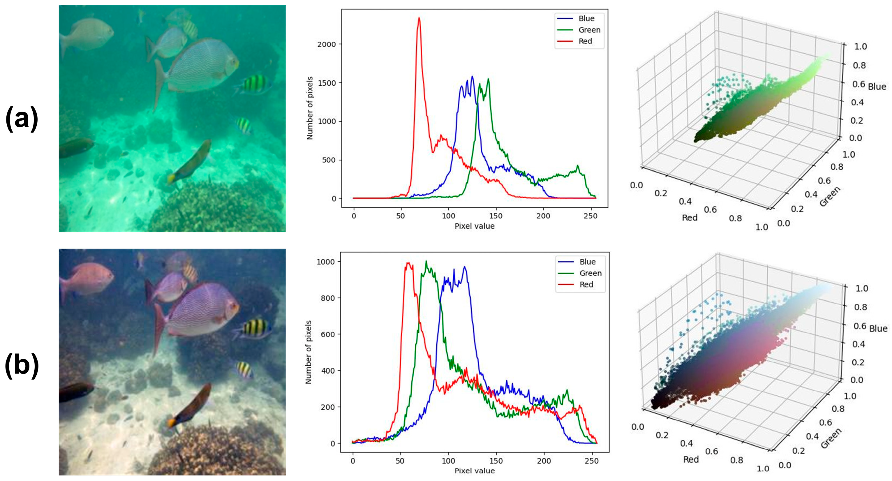
2. Related Work

The underwater robot vision system plays a significant role in exploiting marine resources. However, it is very difficult for these systems to capture high-quality images due to absorption and scattering. Before the emergence of DL-based methods, traditional model-based methods were mainly adopted. Recently, convolution neural network (CNN)- and transformer-based methods have achieved encouraging enhancement results. Considering the model’s overall structure, these methods can be roughly classified into two types: single-branch and multi-branch methods.

Single-branch methods: The single-branch methods usually use a single-path network structure to map the original degraded underwater image to the clear one directly. Liu et al. [6] proposed a residual learning model for the UIE tasks, while an asynchronous training mode was used to boost the performance of the loss function. Chen et al. [13] developed a UIE algorithm based on DL and the image formation model. They constructed the backscatter estimation module and the direct-transmission estimation module using the convolutional neural network’s operation and restored the image using the modified imaging model. Gangisetty et al. [7] designed a novel CNN architecture that improves the residual network structure by leveraging both global and local residual learning approaches. Guo et al. [10] designed a multi-scale dense block for the generator under the framework of generative adversarial networks. A U-shape transformer network was developed by [14], which integrates a channel-wise multi-scale feature fusion transformer module and a spatial-wise global feature modeling transformer module. Although the above methods achieved satisfactory results for UIE, they did not comprehensively consider the complex factors of underwater image degradation. These factors include the color casts caused by absorption and the loss of image details caused by scattering during light propagation in water, making it difficult to mitigate the degradation of complex scenes.

Multi-branch methods: Unlike the single-branch method, the multi-branch method mainly fuses the feature information processed by different branches separately to obtain comprehensive enhancement results. Xue et al. [15] developed a collaborative learning network for luminance and chrominance, which redefines the UIE task as haze removal and color correction sub-tasks by splitting the luminance and chrominance of underwater images. In their subsequent work, Xue et al. [16] designed a multi-branch aggregation network and trained the model to learn a degradation factor to simultaneously achieve color correction and contrast enhancement. Yan et al. [17] developed a multi-branch neural network for the UIE task, which involved the design of an attention-guided dynamic multi-branch block for learning feature representations from different branches. A novel two-branch deep neural network was designed for UIE [18], which could remove the color shifts and improve the visual contrast by fully using the valuable properties of the HSV color space. Jiang et al. [19] considered the factors that affected degradation in underwater images regarding turbidity and chromatism. The authors designed a multi-scale dense boosted module and a deep aesthetic render module to enhance the visual contrast and perform color correction, respectively. Although the aforementioned multi-branch methods have made great progress in terms of visual enhancements, there are still many deficiencies in complex underwater scenes.

DWT-based methods: The discrete wavelet transform technology has good local characteristics in the wavelet domain, and is widely employed in image processing. In recent years, many researchers have integrated DWT technology into DL models to gain more diversified feature information in the wavelet domain. Jamadandi et al. [20] designed an encoder–decoder network with wavelet pooling and unpooling units to solve the issue of UIE. Aytekin et al. [21] developed a denoising network that applied a split convolutional layer to each sub-band of the DWT. Huo et al. [22] proposed a multi-stage model to ameliorate the hybrid degradations progressively, and decomposed the features through the wavelet transform to enhance the details. A wavelet-based two-stream network was designed by [23], which used the DWT to decompose the original signals into low-frequency and high-frequency sub-bands to address the color cast and blurred details of underwater images, respectively. The above-mentioned DWT-based DL network has been successfully applied in image processing tasks, which provides an idea for the model construction in our work.

3. Proposed Method

In this section, the proposed DBFNet framework is introduced in detail. First, an overview of the DBFNet architecture is presented, which comprises three parts: the TCSLB, WDLB, and DASFM. Subsequently, the details of each component of our model are described. Finally, the hybrid loss function adopted during the training of this framework is introduced.

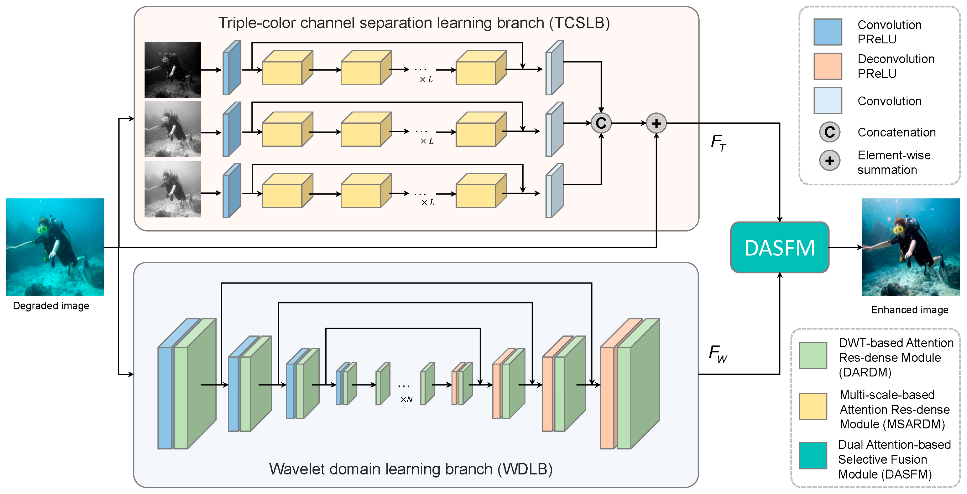
3.1. Overall Architecture

Underwater images inevitably suffer from scattering and absorption when light travels in water, resulting in color casts and detail losses. The UIE task aims to obtain an image with bright colors and clear details from a given input degraded image. However, the underwater scene is intricate, and it is difficult to obtain satisfactory results with general network architectures. As Figure 2 shows, this paper designs a dual-branch fusion architecture. An MSARDM is proposed in the TCSLB, which is applied to the R, G, and B channels, respectively, to learn effective color features. In the WDLB, the detailed features are learned in the wavelet domain by the proposed DARDM. Finally, the two features are reliably merged by the DASFM to produce an underwater image with bright colors and clear details. Mathematically, the whole process can be formulated as:

$$I_{output}={\mathsf{\Phi }}_{DASFM}({\mathsf{\Phi }}_{TCSLB}(I_{input}), {\mathsf{\Phi }}_{\mathrm{WDLB}}(I_{input}))$$

(1)

where $I_{input}$ and $I_{output}$ represent the degraded image and enhanced image, respectively. The symbols ${\mathsf{\Phi }}_{TCSLB}(·)$, ${\mathsf{\Phi }}_{\mathrm{WDLB}}(·)$, and ${\mathsf{\Phi }}_{DASDM}(·)$ represent the modules of the triple-color channel separation learning branch, wavelet domain learning branch, and dual attention-based selective fusion module, respectively.

3.2. Triple-Color Channel Separation Learning Branch (TCSLB)

Since light is absorbed when traveling in water, different color channels have different absorption coefficients that lead to an unbalanced color distribution, resulting in color casts. To alleviate this issue, we design a TCSLB inspired by [12] that uses an MSARDM to process three color channels. Consequently, the network can adapt to adjust the color distribution of the different color channels. For the TCSLB, we use a residual structure and a series of MSARDM groups, which can learn the feature representation according to the different characteristics of the R, G, and B channels, and can adaptively emphasize the latent color information of the three channels. Mathematically, the TCSLB can be formulated as follows:

$$F_{in}^i=\phi (I^i) \mathrm{i}\in \{R, G, B\}$$

(2)

$$F_T^i=Conv(MSARD{M}_n(MSARD{M}_{n-1}\cdot \cdot \cdot MSARD{M}_1(F_{in}^i))+F_{in}^i)$$

(3)

$$F_T=Concat(F_T^R,F_T^G,F_T^B)+I$$

(4)

where $I$ denotes the input image, $I^R, I^G, I^B$ denote the R, G, and B channel of input image,$\phi$ denotes the $P\mathrm{Re}LU(Conv(·))$ operation sequence, and $Concat(·)$ denotes the concatenation operation. The symbol $MSARD{M}_n(·)$ denotes the feature map through the n-th MSARDM, and $F_T^R, F_T^G, F_T^B$ denote the feature maps obtained after feature extraction for the R, G, and B channels, respectively.

Figure 3 illustrates the detailed structure of the MSARDM, which comprises a residual dense block (RDB) and a multi-scale channel attention sub-module. Previous studies have shown that the RDB has been available for feature extraction and can improve the color mapping performance. As Figure 3 shows, the RDB consists of convolutional and PReLU operation sequences. The first N convolutional layers and the PReLU operation sequence aim to boost the number of feature maps, and the purpose of the last layer is to concatenate all feature maps produced from the previous N layer. In our work, N is set to four. A multi-scale channel attention sub-module is introduced at the end of the RDB to enhance the local context feature-capturing ability. Specifically, we first carry out the multi-scale scaling of the feature map $f_{RDB}$ obtained by the RDB, where the scale factors are 1, 1/2, and 1/4. Subsequently, we use these factors in the channel attention to focus on the context features at different scales. Finally, we carry out feature aggregation through the upsampling operation. Given an input feature map $f_{in}$ and output feature map $f_{out}$, the MSARDM is represented as follows:

$$f_{RDB}=RDB(f_{in})$$

(5)

$$\begin{array}{ll}{f}_{out}=& Conv(Concat(CA(f_{RDB}), U{p}_2(CA(Dow{n}_{1/2}(f_{RDB}))), \\ & U{p}_4(CA(Dow{n}_{1/4}(f_{RDB})))))+f_{in}\end{array}$$

(6)

where $U{p}_{\ast }$ and $Dow{n}_{\ast }$ denote the upsampling and downsampling operations, respectively, $RDB(·)$ denotes the residual dense block operation sequence, and CA denotes the channel attention consisting of the $sigmoid(Conv(\mathrm{Re}LU(Conv(GAP(·)))))\otimes ·$ operation sequence.

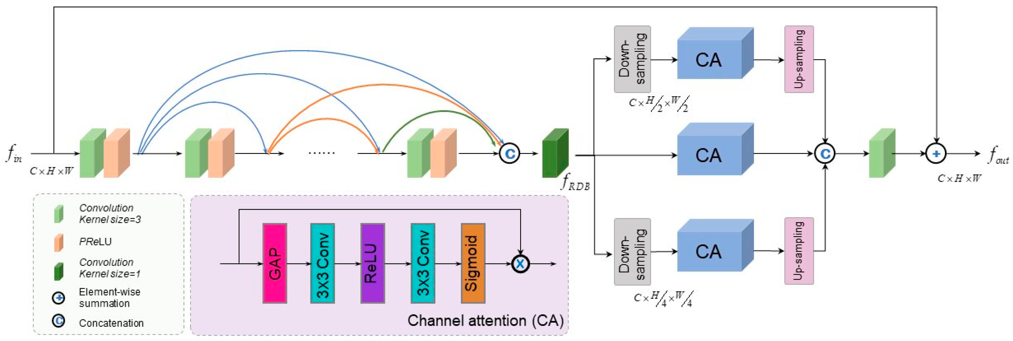
3.3. Wavelet Domain Learning Branch (WDLB)

The wavelet transform is extensively used in traditional image processing methods for denoising and local feature extraction. Recently, deep learning methods based on the DWT techniques have been widely applied in visual processing tasks, such as image deblurring [24], image enhancement [25], and image denoising [26]. For two-dimensional image signals, the horizontal and vertical filtering methods can be used to achieve two-dimensional wavelet decomposition, which results in low-frequency and high-frequency sub-bands. The high-frequency signals usually contain edge and texture information, and the low-frequency signals contain image background information. The DWT can decompose an image into a series of sub-band signals with different frequency characteristics. These sub-signals can supply essential information for the subsequent feature representation and analysis of the model. In addition, the receptive field can be increased while simultaneously preventing information loss, thanks to the reversibility and downsampling properties of the DWT. In this work, we decompose an input using the Haar wavelet transform, which consists of four filters as follows:

$$\begin{array}{cc}{f}_{LL}=\left[\begin{array}{cc}1& 1\\ 1& 1\end{array}\right],& f_{LH}=\left[\begin{array}{cc}-1 & -1\\ 1& 1\end{array}\right]\\ f_{HL}=\left[\begin{array}{cc}-1& 1\\ -1& 1\end{array}\right],& f_{HH}=\left[\begin{array}{cc}1& -1\\ -1& 1\end{array}\right]\end{array}$$

(7)

Thus, given an input I, we can convolve it with the above filters followed by downsampling to obtain four sub-bands: $I_{LL}, I_{LH}, I_{HL}, I_{HH}$, i.e., $I_i=(I\otimes f_i)\downarrow 2, i\in \{LL,LH,HL,HH\}$. According to the bi-orthogonal property of the DWT, the input $I$ can be restored using the IDWT. Therefore, the DWT can be regarded as a convolution operation with a kernel size of $2\times 2$, stride of 2, and fixed weights, while the IDWT is its transposed convolution operation.

Inspired by previous work [22,23,27,28], we designed a wavelet domain learning branch (WDLB) to extract the wavelet domain feature, which uses an encoder–decoder architecture and embeds the DARDM, as shown in Figure 2. Specifically, the WDLB contains three stages: the encoder, bottleneck, and decoder. In the encoder stage, a convolution block (convolution and PReLU) and the designed DARDM are employed to extract the features. In addition, the size of the output feature maps in each encoding stage is halved and the number of channels is doubled. After the encoder stage, a series of DARDMs are cascaded to further refine the encoding features. Finally, in the last stage, a decoder is introduced to restore the feature maps, which consist of a DARDM and a deconvolution block (deconvolution and PReLU). The encoder and decoder operations can be represented as follows:

$$f_{en}^i=DARDM(\phi (f_{en}^{i-1})) \mathrm{i}\in \{1, 2, 3\}$$

(8)

$$f_{de}^i={\phi }^{’}(DARDM(f_{de}^{i-1}))+f_{en}^{3-i} \mathrm{i}\in \{1, 2,3\}$$

(9)

where $f_{en}^i$ and $f_{de}^i$ are the latent features from the encoder and decoder at the i-th layer, respectively; $f_{en}^0$ represents the input image; $f_{de}^0$ represents the output of the bottleneck layer; ${\phi }^{\prime }$ represents the $P\mathrm{Re}LU(DeConv(·))$.

Figure 4 shows the detailed structure of the DARDM, which comprises a dense residual block and a DWT-based attention module. Unlike the RDB in the MSARDM, this base block of the dense residual block comprises a $3\times 3$ convolution layer, BatchNorm layer, and PReLU activation function. In the WDLB, the dense residual block comprises four base blocks and a $1\times 1$ convolution layer. Each prior base block is directly connected to the current base block, and the $1\times 1$ convolution layer is used to handle the output information adaptively. Next, a DWT-based attention module (DAM) is used at the end of the dense residual block to encourage the network to learn the features in the wavelet domain, as illustrated in Figure 4.

Given an intermediate feature map $X_{in}\in {ℝ}^{C\times H\times W}$, the DWT decomposes into half-resolution low-frequency sub-band ($F_{LL}$) and high-frequency ($F_{LH}, F_{HL}, F_{HH}$) sub-bands. Next, these sub-bands are fed to the pixel attention [29] and spatial attention sub-modules, respectively. The low-frequency signal mainly contains structural information, and we use pixel attention to make the model concentrate more on the structural information features. The high-frequency signal mainly contains texture and other details, and we can make the model concentrate more on spatial information features by using spatial attention. After the application of pixel and spatial attention, we can obtain feature maps $F_{LL}^{\prime }$ and $[F_{LH}^{\prime },F_{HL}^{\prime },F_{HH}^{\prime }]$, respectively. Subsequently, we can integrate and reconstruct these sub-bands to the original size by performing the IDWT. Next, we can perform average pooling, convolution, and PReLU operations on the input $X_{in}$ to control the weights of various channel-wise features. Subsequently, these features are passed through the $3\times 3$ convolution layer and PReLU layer to obtain the residual feature $F_r$. Finally, the shortcut features are summed to the residual feature $F_r$ to obtain the output feature map $X_{out}\in {ℝ}^{C\times H\times W}$, which has the DWT-based attention feature information. The mathematical process of the DARDM is as follows:

$$[F_{LL}, F_{LH}, F_{HL}, F_{HH}]=DWT(X_{in})$$

(10)

$$F_{LL}^{\prime }=sigmoid(Conv(\mathrm{Re}LU(Conv(F_{LL}))))\otimes F_{LL}$$

(11)

$$\begin{array}{ll}[F_{LH}^{\prime },F_{HL}^{\prime },F_{HH}^{\prime }]=& sigmoid(Conv([GAP([F_{LH},F_{HL},F_{HH}]);\\ & GMP([F_{LH},F_{HL},F_{HH}])]))\otimes [F_{LH},F_{HL},F_{HH}]\end{array}$$

(12)

$$F_d=IDWT([F_{LL}^{\prime },F_{LH}^{\prime },F_{HL}^{\prime },F_{HH}^{\prime }])$$

(13)

$$F_e=F_d\otimes \phi (Avgpool(X_{in}))$$

(14)

$$X_{out}=\phi (F_e)+X_{in}$$

(15)

where $\phi$ denotes the $P\mathrm{Re}LU(Conv(·))$ operation sequence, and $GAP(·)$ and $GMP(·)$ denote the global average pooling and max pooling, respectively.

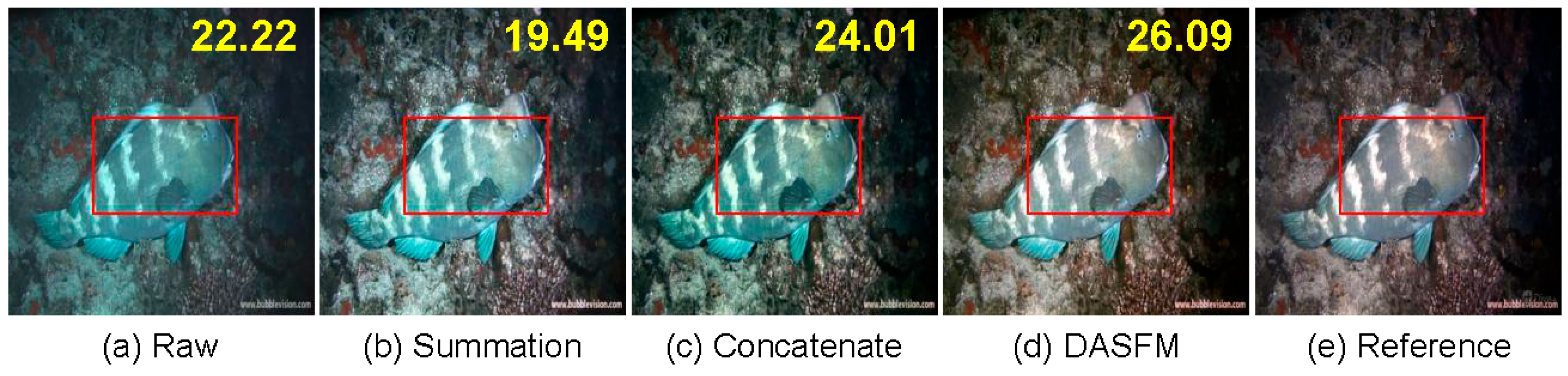
3.4. Dual Attention-Based Selective Fusion Module (DASFM)

In our model, the results from the TCSLB and WDLB contribute differently to the acquisition of high-quality underwater images. In order to fuse these two branches, we design a DASFM inspired by [19,30], which adaptively emphasizes the beneficial feature information of the different branches. Figure 5 shows the corresponding structure. Specifically, the results $F_T$ and $F_W$ from the TCSLB and WDLB, respectively, are first fed into the convolution layer to extract the shallow feature, i.e., $F_t$ and $F_w$, and then concatenated to obtain $F_c$. Second, the pixel attention, channel attention, and convolution layer (convolution and PReLU activation function) are employed to extract the features and obtain the feature maps $F_{cp}$. Third, we feed $F_{cp}$ into the convolution layer and the sigmoid activation function to obtain two attention maps $W_t$ and $W_w$, which are used to adaptively adjust each branch. Last, the feature maps from the dual branches are summed, and the fused feature map is adjusted to the size of the output via a convolution operation. Mathematically, the DASFM can be formulated as:

$$F_t=Conv(F_T), F_w=Conv(F_W)$$

(16)

$$F_c=concat(F_t, F_w)$$

(17)

$$F_{cp}=\phi (concat(CA(F_c), \mathrm{P}A(F_c)))$$

(18)

$$W_t=sigmoid(Conv(F_{cp})), W_w=sigmoid(Conv(F_{cp}))$$

(19)

$$F_{out}=Conv((W_t\otimes F_t)\oplus (W_w\otimes F_w))$$

(20)

where $concat(·)$ denotes the concatenation operation; PA denotes the channel attention, which consists of a $Sigmoid(Conv(\mathrm{Re}LU(Conv(·))))\otimes ·$ operation sequence; and CA denotes pixel attention, which consists of a $Sigmoid(Conv(\mathrm{Re}LU(Conv(GAP(·)))))\otimes ·$ operation sequence.

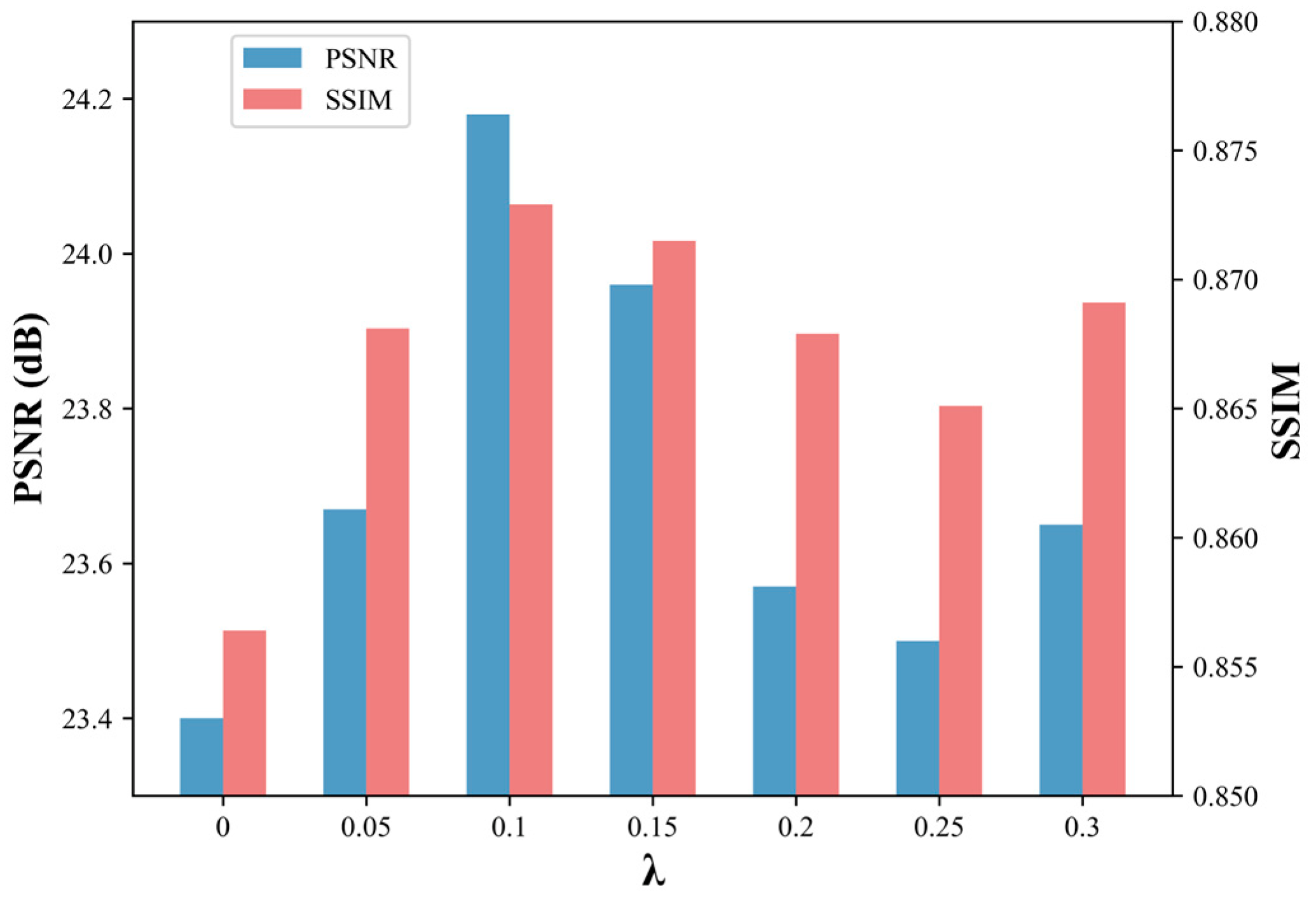
3.5. Hybrid Loss Function

Our DBFNet is trained with the loss function $L_{total}$ that combines the L1 loss $L_{l1}$ and perceptual loss $L_{pre}$ as follows:

$$L_{total}=L_{l1}+\lambda L_{pre}$$

(21)

where $\lambda$ is set to 0.1 to balance different losses, and the details are presented in the ablation study section. Concretely, the L1 loss evaluates the difference between the reconstructed image $I_{recon}$ and the corresponding reference image $I_{ref}$ as:

$$L_{l1}={\displaystyle \sum _{x=1}^H{\displaystyle \sum _{y=1}^W\left|I_{recon}-I_{ref}\right|}}$$

(22)

The perceptual loss [31] is computed based on the VGG-16 network [32] pre-trained on ImageNet. Let ${\varphi }_j(·)$ be the j-th convolutional layer, then ${\varphi }_j(I)$ will be a feature map of shape $C_j\times H_j\times W_j$ when the image I is processed by ${\varphi }_j(·)$. The perceptual loss is the Euclidean distance between the reconstructed image $I_{recon}$ and the corresponding reference image $I_{ref}$, and is expressed as follows:

$$L_{pre}=\frac{1}{C_j{H}_j{W}_j}{‖{\varphi }_j(I_{recon})-{\varphi }_j(I_{ref})‖}_2^2$$

(23)

4. Experiments

In this section, the experimental implementation details are described; then, to verify the performance of our DBFNet, we compare it with nine different recent methods through the described experimental setup and implementation details, and present the visual and quantitative results. Finally, the effectiveness of each component of our DBFNet is verified by an extensive ablation study.

4.1. Experimental Implementation Details

Datasets: The effectiveness of the DBFNet is verified by experiments utilizing publicly available synthetic and real-world underwater datasets. The synthetic dataset is generated from [33], which contains ten water types, labeled as type 1, 3, 5, 7, 9, I, IA, IB, II, and III. Each type consists of 1449 images from the RGB-D NYU-v2 datasets. In our experiments, we select nine water type images as the training and testing datasets, excluding type 9, which is too turbid. We randomly select 1100 samples from each water type. A total of 9900 samples are employed for training, and the remaining 3141 samples are employed as the test set. For the evaluation on real-world underwater images, 800 images from the UIEB are randomly selected [34] for training, and the remaining 90 images are employed as the test set, denoted as Test-90. In addition to 890 degraded–high-quality paired images, the UIEB dataset also contains 60 challenge images for which no corresponding reference images are available. We use these images as the test set, denoted as Test-C60. The resolution of the images is unified both in the training and testing stages.

Experimental settings: The DBFNet is trained using Pytorch as the DL framework on an Nvidia Tesla V100 GPU with 32 Gb of VRAM. Our proposed network is trained using the Adam optimizer with a momentum rate of 0.9. The learning rate is changed according to the cosine annealing strategy [35] with an initial value of 1 × 10⁻⁴. The batch size and the number of epochs are set to 8 and 200, respectively. We empirically set the number of MSARDMs and DARDMs to 5.

Evaluation metrics: For the test set of synthetic datasets and UIEB datasets, we choose three full-reference evaluation metrics, including PSNR [36], SSIM [37], and MSE [38], and two non-reference evaluation metrics, including UIQM [39] and UCIQE [40]. The PSNR and MSE are employed to measure content similarities between the output and reference images; a larger PSNR score or a smaller MSE indicates that the result is similar to the reference image in terms of the contents. The SSIM is employed to measure the contrast and structure similarity; a larger SSIM value indicates that the result is closer to the reference image in terms of the texture and structure. Its definition is given by:

$$\mathrm{SSIM}(\mathrm{x},\mathrm{y})=\frac{(2{\mu }_x{\mu }_y+{\mathrm{c}}_1)(2{\sigma }_x{\sigma }_y+{\mathrm{c}}_2)}{({\mu }_x^2+{\mu }_y^2+{\mathrm{c}}_1)({\sigma }_x^2+{\sigma }_y^2+{\mathrm{c}}_2)}$$

(24)

where ${\mu }_x$ and ${\sigma }_x$ represent the mean and variance of x, respectively; ${\mu }_y$ and ${\sigma }_y$ represent the mean and variance of y, respectively; ${\sigma }_{xy}$ represents the cross-correlation between x and y; $c_1$ and $c_2$ are fixed constants.

The UIQM has a stronger correlation with human visual perception, which includes three attribute measures, i.e., the underwater image color metric (UICM), underwater image sharpness metric (UISM), and underwater image contrast metric (UIConM). Its definition is given by:

$$\mathrm{UIQM}={\mathrm{c}}_1\times \mathrm{UICM}+{\mathrm{c}}_2\times \mathrm{UISM}+{\mathrm{c}}_3\times \mathrm{UIConM}$$

(25)

where ${\mathrm{c}}_1=0.0282$, ${\mathrm{c}}_2=0.2953$, and ${\mathrm{c}}_3=3.5753$ are set according to [39].

The UIQM and UCIQE are employed to measure the non-uniform color shift and contrast of output images; a larger UIQM value or a larger UCIQE value indicates a better visual effect.

Comparison methods: The performance achieved by DBFNet is demonstrated by comparing it with nine recent state-of-the-art (SOTA) methods, including traditional methods (UDCP [1], IBLA [2]) and DL-based methods (Shallow-UWnet [41], Chen et al.’s method [13], UResnet [6], WaterNet [34], Deep-WaveNet [42], UGAN [43], Ma et al.’s method [23]).

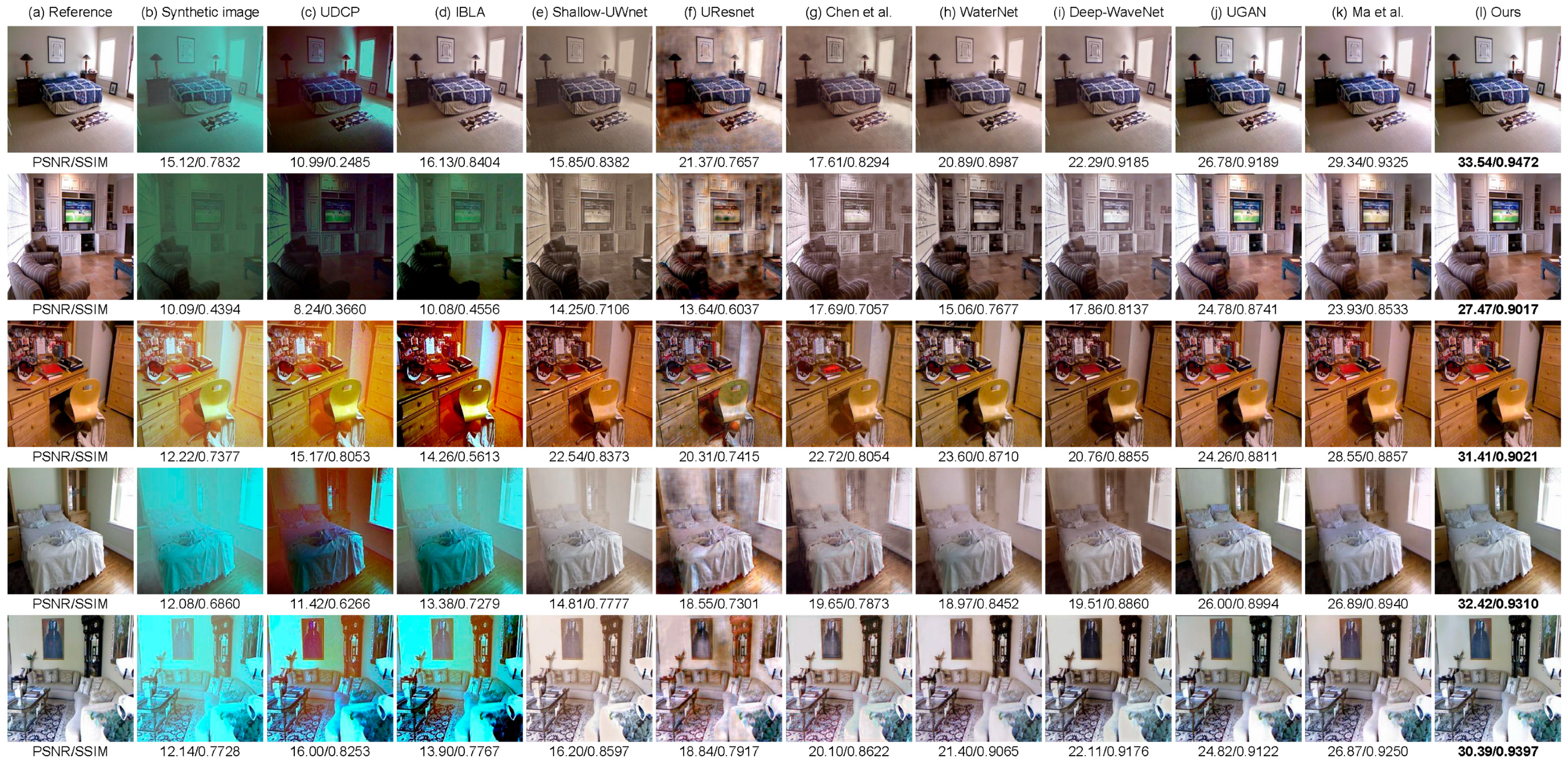
4.2. Comparisons on Synthetic Datasets

As reference underwater images are difficult to obtain, many researchers train and test deep learning models using synthetic underwater image datasets.

Table 1. Quantitative comparison results of various UIE approaches on the synthetic underwater dataset in terms of PSNR (dB), SSIM, and MSE ($\times {10}^3$) values. We present the optimal and suboptimal results with values in bold and underlined, respectively.

Types	Metrics	UDCP	IBLA	Shallow-UWnet	UResnet	Chen et al.	WaterNet	Deep-WaveNet	UGAN	Ma et al.	Ours
1	PSNR	13.68	14.70	18.85	19.50	20.07	20.67	23.08	25.45	27.82	31.93
	SSIM	0.6547	0.6881	0.7789	0.7158	0.7518	0.8361	0.8651	0.8874	0.8873	0.9165
	MSE	3.3332	2.8291	1.3059	0.9665	0.8480	0.7702	0.4172	0.1914	0.1279	0.0464
3	PSNR	11.84	13.03	15.04	16.71	17.43	17.97	19.76	24.74	24.58	29.68
	SSIM	0.5444	0.0639	0.6863	0.6492	0.6908	0.7825	0.7972	0.8616	0.8434	0.8962
	MSE	4.9485	3.6553	2.2795	1.7687	1.4022	1.3724	0.9074	0.2353	0.3010	0.0895
5	PSNR	10.00	11.16	13.80	13.34	15.40	15.13	16.52	22.61	20.91	24.95
	SSIM	0.3992	0.4531	0.6118	0.5079	0.6059	0.6955	0.6997	0.7863	0.7671	0.8356
	MSE	7.4906	5.7544	3.0015	3.3493	2.1646	2.4177	1.7984	0.4646	0.7468	0.3420
7	PSNR	8.99	9.73	13.05	11.33	13.97	13.44	14.43	19.11	17.43	20.01
	SSIM	0.2775	0.3197	0.5285	0.3884	0.5272	0.6025	0.5920	0.6322	0.6590	0.7185
	MSE	9.7561	8.5102	3.5799	5.1834	3.0144	3.4888	2.8472	1.1833	1.6848	1.1682
I	PSNR	16.53	14.13	21.98	20.70	23.67	24.06	25.95	25.57	29.72	33.00
	SSIM	0.7640	0.5591	0.8495	0.7374	0.8339	0.8847	0.9149	0.8934	0.9069	0.9247
	MSE	1.6850	2.9865	0.5588	0.7715	0.3316	0.3295	0.1998	0.1856	0.0769	0.0353
IA	PSNR	16.72	14.37	22.14	21.22	23.74	24.16	26.03	25.63	29.90	32.89
	SSIM	0.7747	0.5804	0.8554	0.7532	0.8405	0.8884	0.9197	0.8964	0.9106	0.9257
	MSE	1.6099	2.9442	0.4847	0.6348	0.3161	0.3140	0.1940	0.1836	0.0740	0.0360
IB	PSNR	16.44	14.53	21.95	21.10	23.29	23.41	25.75	25.59	29.78	32.76
	SSIM	0.7661	0.5998	0.8448	0.7479	0.8260	0.8770	0.9109	0.8951	0.9060	0.9231
	MSE	1.7255	2.8851	0.5305	0.6578	0.3587	0.3832	0.2074	0.1842	0.0768	0.0372
II	PSNR	15.55	15.29	21.01	21.06	21.81	22.78	24.90	25.58	29.29	32.70
	SSIM	0.7384	0.6763	0.8216	0.7494	0.7978	0.8657	0.8992	0.8957	0.9015	0.9227
	MSE	2.1428	2.5699	0.7549	0.6544	0.5353	0.4471	0.2567	0.1843	0.0888	0.0380
III	PSNR	13.67	14.92	18.2	19.43	19.84	20.13	22.64	25.46	27.44	31.91
	SSIM	0.6639	0.7035	0.776	0.7220	0.7578	0.8345	0.8681	0.8906	0.8869	0.9186
	MSE	3.3143	2.5748	1.4835	1.0180	0.9028	0.8556	0.4515	0.1908	0.1392	0.0461

presents the quantitative results of the PSNR, SSIM, and MSE for underwater images of nine different water types, where the bold and underlined scores show the optimal and sub-optimal results. It can be observed that our DBFNet obtains the highest score for the PSNR, SSIM, and MSE metrics in all water types. This shows that our DBFNet can effectually enhance the image contrast, correct the image color, and perform well in detail retention. In addition, in terms of these three evaluation metrics, our DBFNet is obviously superior to the comparative method, with absolute advantages.

Figure 6 presents the visual results of our DBFNet versus the comparison method on the synthesized underwater dataset. It can be observed that the UDCP and IBLA perform poorly in terms of the image contrast improvement and color correction, and even aggravate image degradation, which may be because these methods rely on prior knowledge. Although DL-based methods can obtain relatively better results, a few methods, such as Shallow-UWnet, UResnet, and Chen et al.’s method, are prone to artifacts and blurring. In contrast, WaterNet, Deep-WaveNet, UGAN, Ma et al.’s method, and our proposed method can achieve relatively good visual results. However, WaterNet and Deep-WaveNet show poor color correction performance, as presented in the second column of Figure 6. It is obvious that our result is similar to the reference image than the comparison methods, and our DBFNet has good performance for color correction and detail preservation. Moreover, as presented in Figure 6, our model produces the highest PSNR and SSIM scores among the compared methods, which further demonstrates the effectiveness of the DBFNet.

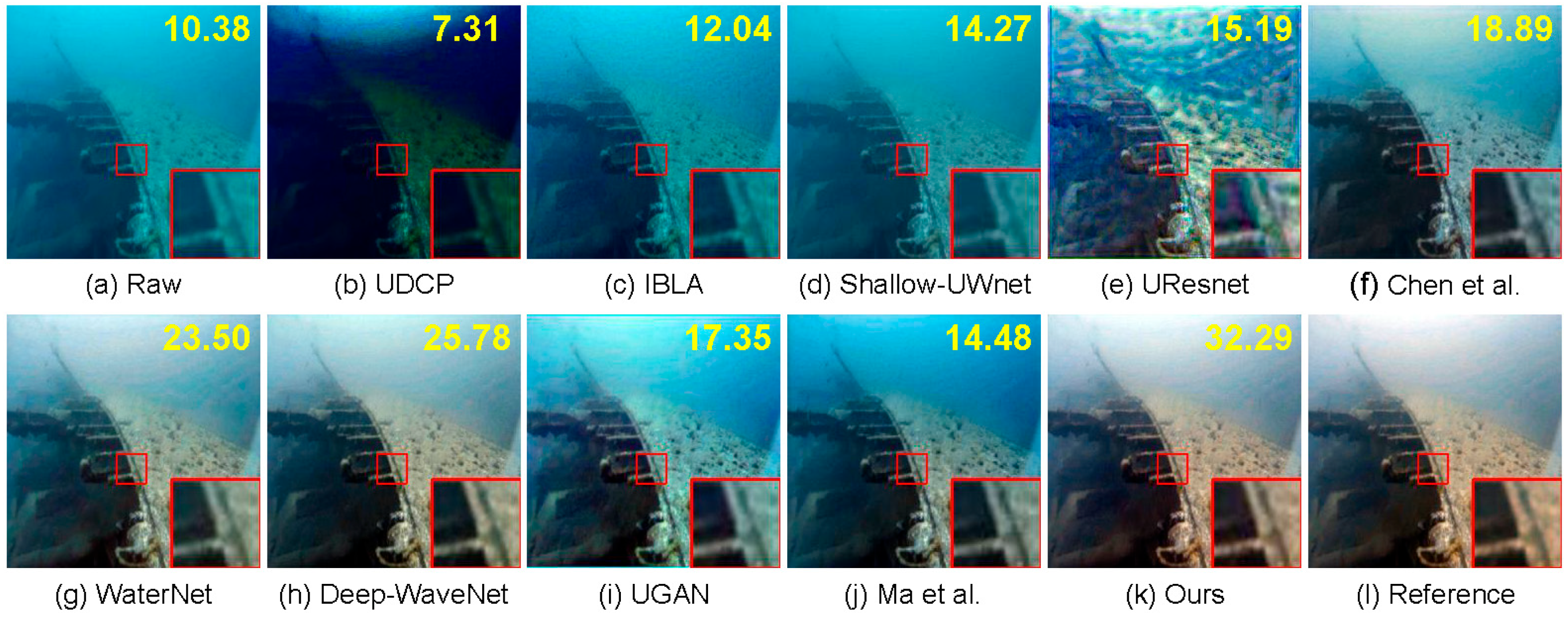
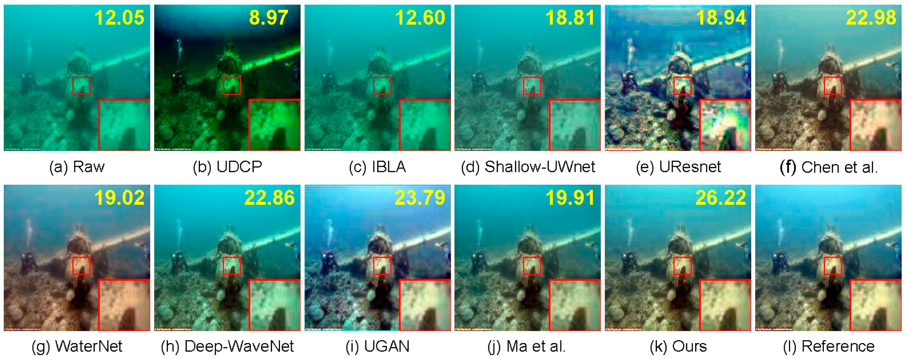
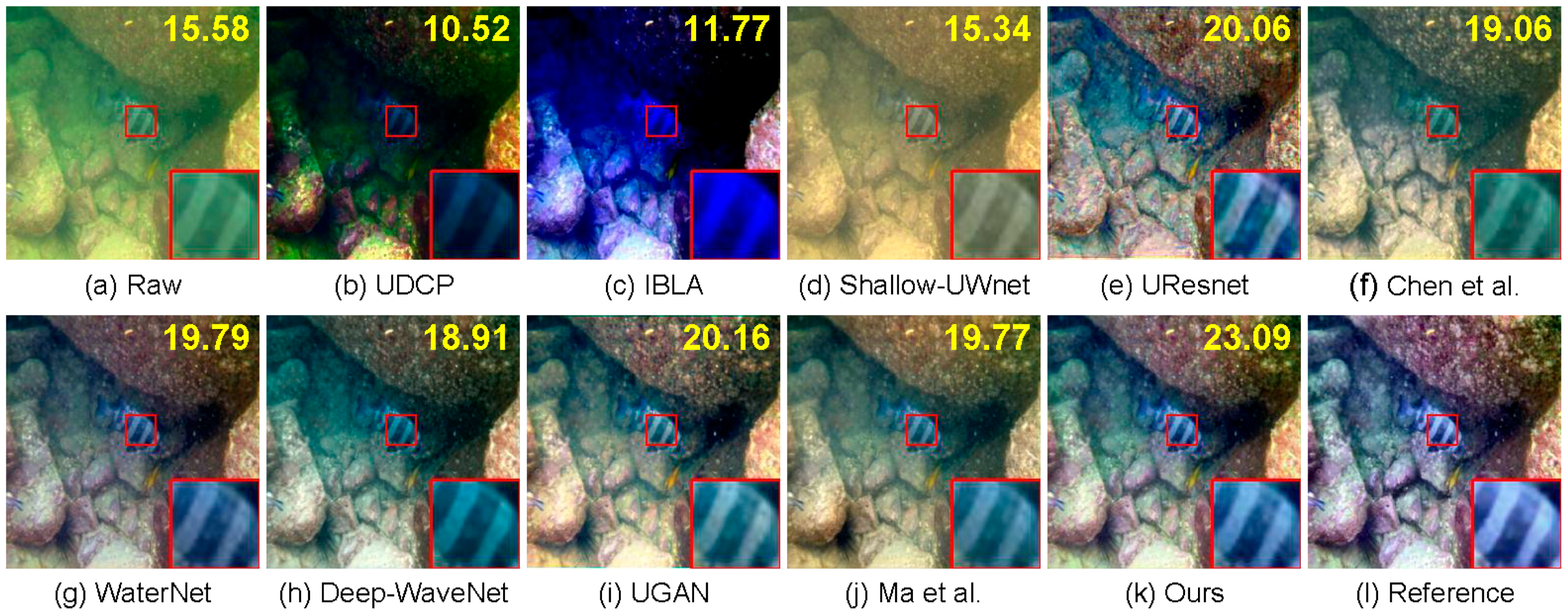
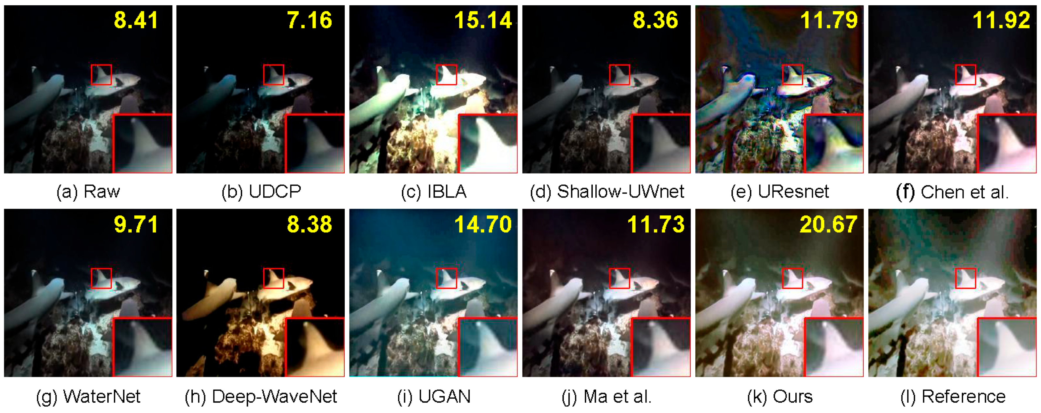
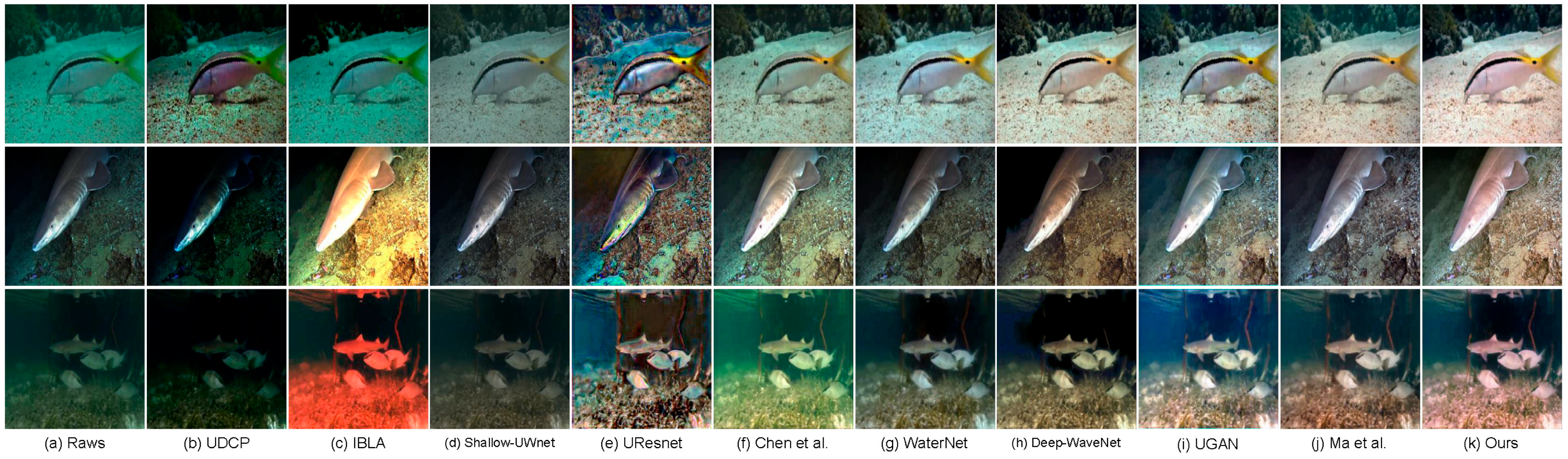
4.3. Comparisons on Real-World Datasets

Visual comparisons: Due to the absorption and scattering of light traveling through the water, the image often produces color casts and suffers from a loss of detail. To verify the performance of our DBFNet in color correction and detail restoration, inspired by [44], we divide the images of the Test-90 dataset into five categories: bluish, greenish, yellow tone, shallow water, and low-illuminated images, as present in Figure 7, Figure 8, Figure 9, Figure 10 and Figure 11.

From the perspective of the color correction performance, the UDCP and IBIA are ineffective in eliminating the color offset and enhancing the visual contrast, which may be due to the low robustness of the traditional methods in complex underwater images. The Shallow-UWnet and UResnet methods slightly improve the color shifts, but do not eliminate the severe color bias. In addition, UResnet introduces extra background noise. The other methods have different color correction performances, but the WaterNet method can easily over-enhance the color correction, and Chen et al.’s method, the Deep-WaveNet method, the UGAN method, and Ma et al.’s method cannot completely eliminate the color casts. Figure 7, Figure 8, Figure 9, Figure 10 and Figure 11 show that our DBFNet can produce the best color correction performance.

From the perspective of the detail restoration performance, the UDCP, IBLA, and Shallow-UWnet methods perform poorly due to the interference from color casts. The UResnet is affected by the introduction of additional background noise, and the level of detail is not clearly restored. The remaining methods affect the restoration of details to some extent, although a few methods such as Chen et al.’s method, the WaterNet method, the UGAN method, and Ma et al. method are affected by color offset and haze, rendering poor results, as shown in Figure 7 and Figure 9. The comparison results demonstrate that our DBFNet produces the best detail restoration results and improves the brightness and saturation of the underwater images.

The robustness of the proposed DBFNet is verified by conducting comparative experiments on the challenging test set, i.e., Test-C60, whose visual effects are shown in Figure 12. We can observe that the traditional methods perform poorly, the UDCP reduces the image contrast, and the IBLA aggravates the color casts. The Shallow-UWnet has a slight enhancement effect, UResnet gives rise to extra background noise, and Chen et al.’s method result in over-enhancement. The UGAN method, Ma et al.’s method, and our method show good enhancement performance. Out of these methods, our method performs better in brightness improvement.

Quantitative evaluation: For the quantitative evaluation, we use the fully referenced evaluation metrics and the non-referenced evaluation metrics for the fully referenced images in the Test-90 and the non-referenced images in Test-C60, respectively. We calculate the average scores of all images in the corresponding dataset, and the results are presented in

Table 2. Quantitative comparison results of various UIE approaches on the Test-90 dataset in terms of PSNR (dB), SSIM, and MSE ($\times {10}^3$). We present the optimal and sub-optimal results with values in bold and underlined, respectively.

Methods	$\mathbf{PSNR}\uparrow$	$\mathbf{SSIM}\uparrow$	$\mathbf{MSE}\downarrow$
UDCP	11.51	0.5212	5.1332
IBLA	15.81	0.6651	2.8412
Shallow-UWnet	17.79	0.7403	1.6002
UResnet	18.32	0.7175	1.1126
Chen et al.	21.32	0.8260	0.6588
WaterNet	20.88	0.8418	0.7840
Deep-WaveNet	22.34	0.8656	0.7030
UGAN	20.43	0.8255	0.6836
Ma et al.	20.04	0.8305	0.8495
Ours	24.18	0.8729	0.4054

and

Table 3. Quantitative comparison results of various UIE approaches on the Test-C60 dataset. We present the best, second-best, and third-best results with values in bold, underlined, and double underlined, respectively.

Methods	$\mathbf{UICM}\uparrow$	$\mathbf{UISM}\uparrow$	$\mathbf{UIConM}\uparrow$	$\mathbf{UIQM}\uparrow$	$\mathbf{UCIQE}\uparrow$
UDCP	5.3511	3.8881	0.0472	1.4679	0.5364
IBLA	5.8522	4.3957	0.1627	2.0448	0.5685
Shallow-UWnet	2.0769	4.2078	0.2842	2.3172	0.4677
UResnet	6.7992	6.4352	0.1976	2.7986	0.5974
Chen et al.	4.5519	5.3269	0.2821	2.7099	0.5466
WaterNet	4.1166	5.2974	0.2620	2.6172	0.5698
Deep-WaveNet	4.2254	5.1885	0.2499	2.5450	0.5729
UGAN	5.4232	6.0859	0.2591	2.8766	0.6037
Ma et al.	3.8633	5.2574	0.2851	2.6809	0.5473
Ours	5.1320	5.5205	0.2678	2.7326	0.5827

. As Table 2 shows, our proposed DBFNet obtains the best PSNR, SSIM, and MSE scores. Compared with the Deep-WaveNet (suboptimal method), our DBFNet achieves gains of 8.2% and 0.8% in terms of the PSNR and SSIM metrics, respectively. Table 3 presents the comparison results of non-referenced measures. It can be observed that our DBFNet obtains third-best results with respect to the UISM, UIQM, and UCIQE metrics. Although the UResnet and UGAN methods perform well for these metrics, from the perspective of visual results, there is serious background noise in the results obtained using the UResnet, which is obviously unwanted. It should be noted that there is a certain difference between the visual effects and the quantitative values in some cases, which is also confirmed in [45,46]. Therefore, based on the combined visual comparison and quantitative evaluation, our DBFNet achieves better performance.

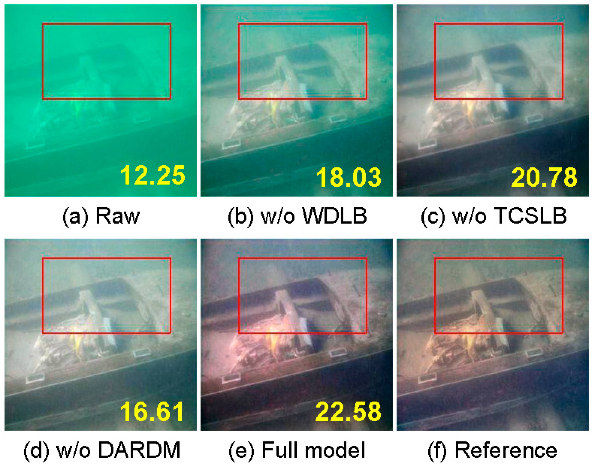
4.4. Ablation Studies

In this section, we perform ablation studies on UIEB datasets, based on a Nvidia Tesla V100 GPU with 32 Gb of VRAM. The same training and testing datasets and parameter settings are used for all ablation studies.

Parameter selection of the loss function: The validity of the parameters of the loss function used in our work is verified by calculating the PSNR and SSIM values under various values of λ on the Test-90 dataset, and the quantitative results are presented in Figure 13. It can be clearly seen that the best performance is obtained when λ is equal to 0.1.

Effectiveness of the network components: The validity of each of our developed modules is verified by designing appropriate ablation studies. The visual and quantitative results are presented in Figure 14 and

Table 4. Quantitative comparison results of the ablation study of the components of DBFNet in terms of PSNR (dB), SSIM, and MSE ($\times {10}^3$) values. Bold values indicate the best results.

Methods	w/o WDLB	w/o TCSLB	w/o DARDM	Full Model
PSNR	21.39	23.40	22.89	24.18
SSIM	0.8434	0.8573	0.8584	0.8729
MSE	0.6466	0.4501	0.5006	0.4054

, respectively. In these results, w/o WDLB, w/o TCSLB, and w/o DARDM denote the proposed model without WDLB, without TCSLB, and without DARDM, respectively. As presented in Table 4, our full model achieves the highest score for all evaluation metrics for the ablated models. As shown in Figure 14, especially in the red rectangular box, our full model achieves the best visual effect in terms of detail preservation and color correction. It can be further observed from Figure 14 that although the color can be mostly corrected when the WDLB, TCLSB, or DARDM is removed from the full model, different degrees of haze are produced and the details are unclear. Combining the quantitative and qualitative results, it can be observed that our proposed components play a significant role in the performance of the full model.

Effectiveness of the fusion method: We verify the effectiveness of the DASFM by comparing it with two other commonly used fusion methods, i.e., element-wise summation and concatenation. As

Table 5. Quantitative comparison results of ablation study of the dual-branch fusion methods in terms of PSNR (dB), SSIM, and MSE ($\times {10}^3$) values. Bold values indicate the best results.

Methods	Summation	Concatenate	DASFM
PSNR	23.25	23.95	24.18
SSIM	0.8688	0.8710	0.8729
MSE	0.4446	0.3934	0.4054

shows, the DASFM gets the highest scores in terms of the PSNR and SSIM metrics compared with the other fusion methods, while the MSE metric is slightly weaker than the concatenated fusion method. As Figure 15 shows, especially in the red rectangular box, compared with the other two fusion methods, the DASFM achieves better visual performance, the result is similar to the reference image, and the interference of blue haze can be effectively eliminated.

5. Conclusions

In this work, we developed a novel dual-branch fusion network for UIE, which contains three components, including a triple-color channel separation learning branch, a wavelet domain learning branch, and a dual attention-based selective fusion module. Firstly, an MSARDM was designed to learn the color feature in three channels independently to balance the color distribution. Secondly, a DARDM was designed to make the most of learning the wavelet domain information, which can protect the details of the information. Finally, a DASFM was designed to adapt the fusion the beneficial results from two branches. Our extensive quantitative and visualization evaluations on synthetic and real-world underwater datasets have demonstrated that the proposed DBFNet performs better than other methods.

However, the DBFNet still has some limitations. The dual attention-based selective fusion module we designed shows limited improvements compared with the concatenated operation. In future studies, we hope to enhance the study of the fusion module for better visual results.

References

1. Drews, P.; Nascimento, E.; Moraes, F.; Botelho, S.; Campos, M. Transmission Estimation in Underwater Single Images. In Proceedings of the IEEE International Conference on Computer Vision Workshops, Sydney, Australia, 1–8 December 2013; pp. 825–830. [Google Scholar]
2. Peng, Y.-T.; Cosman, P.C. Underwater image restoration based on image blurriness and light absorption. IEEE Trans. Image Process. 2017, 26, 1579–1594. [Google Scholar] [CrossRef] [PubMed]
3. Zhou, J.; Liu, D.; Xie, X.; Zhang, W. Underwater image restoration by red channel compensation and underwater median dark channel prior. Appl. Optics 2022, 61, 2915–2922. [Google Scholar] [CrossRef] [PubMed]
4. Liu, S.; Fan, H.; Lin, S.; Wang, Q.; Ding, N.; Tang, Y. Adaptive Learning Attention Network for Underwater Image Enhancement. IEEE Robot. Autom. Lett. 2022, 7, 5326–5333. [Google Scholar] [CrossRef]
5. Li, Y.; Chen, R. UDA-Net: Densely Attention Network for Underwater Image Enhancement. IET Image Process. 2021, 15, 774–785. [Google Scholar] [CrossRef]
6. Liu, P.; Wang, G.; Qi, H.; Zhang, C.; Zheng, H.; Yu, Z. Underwater image enhancement with a deep residual framework. IEEE Access 2019, 7, 94614–94629. [Google Scholar] [CrossRef]
7. Gangisetty, S.; Rai, R.R. FloodNet: Underwater image restoration based on residual dense learning. Signal Process. Image Commun. 2022, 104, 116647. [Google Scholar] [CrossRef]
8. Yang, H.H.; Huang, K.C.; Chen, W.T. LAFFNet: A lightweight adaptive feature fusion network for underwater image enhancement. In Proceedings of the IEEE International Conference on Robotics and Automation (ICRA), Xi’an, China, 30 May–5 June 2021; pp. 685–692. [Google Scholar]
9. Qi, Q.; Zhang, Y.; Tian, F.; Wu, Q.M.J.; Li, K.; Luan, X.; Song, D. Underwater image co-enhancement with correlation feature matching and joint learning. IEEE Trans. Circuits Syst. Video Technol. 2021, 32, 1133–1147. [Google Scholar] [CrossRef]
10. Guo, Y.; Li, H.; Zhuang, P. Underwater image enhancement using a multiscale dense generative adversarial network. IEEE J. Oceanic Eng. 2019, 45, 862–870. [Google Scholar] [CrossRef]
11. Yang, M.; Hu, K.; Du, Y.; Wei, Z.; Sheng, Z.; Hu, J. Underwater image enhancement based on conditional generative adversarial network. Signal Process. Image Commun. 2020, 81, 115723. [Google Scholar] [CrossRef]
12. Zhang, D.; Shen, J.; Zhou, J.; Chen, E.; Zhang, W. Dual-path joint correction network for underwater image enhancement. Opt. Express 2022, 30, 33412–33432. [Google Scholar] [CrossRef]
13. Chen, X.; Zhang, P.; Quan, L.; Yi, C.; Lu, C. Underwater image enhancement based on deep learning and image formation model. arXiv 2021, arXiv:2101.00991. [Google Scholar]
14. Peng, L.; Zhu, C.; Bian, L. U-shape Transformer for Underwater Image Enhancement. arXiv 2021, arXiv:2111.11843. [Google Scholar]
15. Xue, X.; Hao, Z.; Ma, L.; Wang, Y.; Liu, R. Joint luminance and chrominance learning for underwater image enhancement. IEEE Signal Process. Lett. 2021, 28, 818–822. [Google Scholar] [CrossRef]
16. Xue, X.; Li, Z.; Ma, L.; Jia, Q.; Liu, R.; Fan, X. Investigating intrinsic degradation factors by multi-branch aggregation for real-world underwater image enhancement. Pattern Recognit. 2023, 133, 109041. [Google Scholar] [CrossRef]
17. Yan, X.; Qin, W.; Wang, Y.; Wang, G.; Fu, X. Attention-guided dynamic multi-branch neural network for underwater image enhancement. Knowl.-Based Syst. 2022, 258, 110041. [Google Scholar] [CrossRef]
18. Hu, J.; Jiang, Q.; Cong, R.; Gao, W.; Shao, F. Two-branch deep neural network for underwater image enhancement in HSV color space. IEEE Signal Process. Lett. 2021, 28, 2152–2156. [Google Scholar] [CrossRef]
19. Jiang, Z.; Li, Z.; Yang, S.; Gao, W.; Shao, F. Target Oriented Perceptual Adversarial Fusion Network for Underwater Image Enhancement. IEEE Trans. Circuits Syst. Video Technol. 2022, 32, 6584–6598. [Google Scholar] [CrossRef]
20. Jamadandi, A.; Mudenagudi, U. Exemplar-based underwater image enhancement augmented by wavelet corrected transforms. In Proceedings of the IEEE/CVF Conference on Computer Vision and Pattern Recognition Workshops, Long Beach, CA, USA, 15–21 June 2019; pp. 11–17. [Google Scholar]
21. Aytekin, C.; Alenius, S.; Paliy, D.; Gren, J. A Sub-band Approach to Deep Denoising Wavelet Networks and a Frequency-adaptive Loss for Perceptual Quality. In Proceedings of the IEEE International Workshop on Multimedia Signal Processing, Tampere, Finland, 6–8 October 2021; pp. 1–6. [Google Scholar]
22. Huo, F.; Li, B.; Zhu, X. Efficient Wavelet Boost Learning-Based Multi-stage Progressive Refinement Network for Underwater Image Enhancement. In Proceedings of the IEEE/CVF International Conference on Computer Vision, Montreal, BC, Canada, 11–17 October 2021; pp. 1944–1952. [Google Scholar]
23. Ma, Z.; Oh, C. A Wavelet-Based Dual-Stream Network for Underwater Image Enhancement. In Proceedings of the IEEE International Conference on Acoustics, Speech and Signal Processing (ICASSP), Singapore, 23–27 May 2022; pp. 2769–2773. [Google Scholar]
24. Zou, W.; Jiang, M.; Zhang, Y.; Chen, L.; Lu, Z.; Wu, Y. SDWnet: A straight dilated network with wavelet transformation for image deblurring. In Proceedings of the IEEE/CVF International Conference on Computer Vision, Montreal, BC, Canada, 11–17 October 2021; pp. 1895–1904. [Google Scholar]
25. Fan, C.M.; Liu, T.J.; Liu, K.H. Half Wavelet Attention on M-Net+ for Low-Light Image Enhancement. arXiv 2022, arXiv:2203.01296. [Google Scholar]
26. Peng, Y.; Cao, Y.; Liu, S.; Yang, J.; Zuo, W. Progressive training of multi-level wavelet residual networks for image denoising. arXiv 2020, arXiv:2010.12422. [Google Scholar]
27. Zhang, Y.; Li, K.; Li, K.; Wang, L.; Zhong, B.; Fu, Y. Image super-resolution using very deep residual channel attention networks. In Proceedings of the European Conference on Computer Vision (ECCV), Munich, Germany, 8–14 September 2018; pp. 286–301. [Google Scholar]
28. Sun, K.; Meng, F.; Tian, Y. Underwater image enhancement based on noise residual and color correction aggregation network. Digit. Signal Process. 2022, 129, 103684. [Google Scholar] [CrossRef]
29. Qin, X.; Wang, Z.; Bai, Y.; Xie, X.; Jia, H. FFA-Net: Feature fusion attention network for single image dehazing. In Proceedings of the AAAI Conference on Artificial Intelligence, New York, NY, USA, 7–12 February 2020; pp. 11908–11915. [Google Scholar]
30. Yang, H.; Zhou, D.; Cao, J.; Zhao, Q. DPNet: Detail-preserving image deraining via learning frequency domain knowledge. Digit. Signal Process. 2022, 130, 103740. [Google Scholar] [CrossRef]
31. Johnson, J.; Alahi, A.; Fei-Fei, L. Perceptual losses for real-time style transfer and super-resolution. In Proceedings of the European Conference on Computer Vision, Amsterdam, The Netherlands, 8–16 October 2016; pp. 694–711. [Google Scholar]
32. Simonyan, K.; Zisserman, A. Very deep convolutional networks for large-scale image recognition. arXiv 2014, arXiv:1409.1556. [Google Scholar]
33. Anwar, S.; Li, C.; Porikli, F. Deep underwater image enhancement. arXiv 2018, arXiv:1807.03528. [Google Scholar]
34. Li, C.; Guo, C.; Ren, W.; Cong, R.; Hou, J.; Kwong, S.; Tao, D. An underwater image enhancement benchmark dataset and beyond. IEEE Trans. Image Process. 2019, 29, 4376–4389. [Google Scholar] [CrossRef] [Green Version]
35. Loshchilov, I.; Hutter, F. SGDR: Stochastic gradient descent with warm restarts. arXiv 2016, arXiv:1608.03983. [Google Scholar]
36. Hore, A.; Ziou, D. Image Quality Metrics: PSNR vs. SSIM. In Proceedings of the International Conference on Pattern Recognition, Istanbul, Turkey, 23–26 August 2010; pp. 2366–2369. [Google Scholar]
37. Wang, Z.; Bovik, A.C.; Sheikh, H.R.; Simoncelli, E.P. Image Quality Assessment: From Error Visibility to Structural Similarity. IEEE Trans. Image Process. 2004, 13, 600–612. [Google Scholar] [CrossRef] [Green Version]
38. Hunt, B.R. The Application of Constrained Least Squares Estimation to Image Restoration by Digital Computer. IEEE Trans. Comput. 1973, 100, 805–812. [Google Scholar] [CrossRef]
39. Panetta, K.; Gao, C.; Agaian, S. Human-visual-system-inspired Underwater Image Quality Measures. IEEE J. Ocean. Eng. 2015, 41, 541–551. [Google Scholar] [CrossRef]
40. Yang, M.; Sowmya, A. An Underwater Color Image Quality Evaluation Metric. IEEE Trans. Image Process. 2015, 24, 6062–6071. [Google Scholar] [CrossRef]
41. Naik, A.; Swarnakar, A.; Mittal, K. Shallow-UWnet: Compressed Model for Underwater Image Enhancement. In Proceedings of the AAAI Conference on Artificial Intelligence, Vancouver, BC, Canada, 2–9 February 2021; pp. 15853–15854. [Google Scholar]
42. Sharma, P.K.; Bisht, I.; Sur, A. Wavelength-based Attributed Deep Neural Network for Underwater Image Restoration. arXiv 2021, arXiv:2106.07910. [Google Scholar] [CrossRef]
43. Fabbri, C.; Islam, M.J.; Sattar, J. Enhancing underwater imagery using generative adversarial networks. In Proceedings of the IEEE International Conference on Robotics and Automation, Brisbane, Australia, 21–25 May 2018; pp. 7159–7165. [Google Scholar]
44. Wang, Y.; Guo, J.; Gao, H.; Yue, H. UIEC2Net: CNN-based Underwater Image Enhancement Using Two Color Space. Signal Process. Image Commun. 2021, 96, 116250. [Google Scholar] [CrossRef]
45. Chen, L.; Jiang, Z.; Tong, L.; Liu, Z.; Zhao, A.; Zhang, Q.; Dong, J.; Zhou, H. Perceptual underwater image enhancement with deep learning and physical priors. IEEE Trans. Circuits Syst. Video Technol. 2020, 31, 3078–3092. [Google Scholar] [CrossRef]
46. Liu, R.; Fan, X.; Zhu, M.; Hou, M.; Luo, Z. Real-world underwater enhancement: Challenges, benchmarks, and solutions under natural light. IEEE Trans. Circuits Syst. Video Technol. 2020, 30, 4861–4875. [Google Scholar] [CrossRef]
Figure 1. An example of the color distribution of an underwater raw image and its corresponding enhanced image: (a) raw image and its tricolor histogram and three-dimensional color distribution; (b) enhanced image and its tricolor histogram and three-dimensional color distribution.
Remotesensing 15 01195 g001
Figure 2. The architecture of our proposed DBFNet for UIE.
Remotesensing 15 01195 g002
Figure 3. Illustration of the MSARDM in the TCSLB.
Remotesensing 15 01195 g003
Figure 4. Illustration of the DARDM in the WDLB.
Remotesensing 15 01195 g004
Figure 5. Illustration of the DASFM.
Remotesensing 15 01195 g005
Figure 6. Visual comparisons of synthetic underwater images.
Remotesensing 15 01195 g006
Figure 7. The visual comparisons of various UIE approaches on the bluish underwater images. The number on each image represents its PSNR score.
Remotesensing 15 01195 g007
Figure 8. The visual comparisons of various UIE approaches on greenish underwater images. The number on each image represents its PSNR score.
Remotesensing 15 01195 g008
Figure 9. The visual comparisons of various UIE approaches on the yellowish underwater images. The number on each image represents its PSNR score.
Remotesensing 15 01195 g009
Figure 10. The visual comparisons of various UIE approaches on shallow water images. The number on each image represents its PSNR score.
Remotesensing 15 01195 g010
Figure 11. The visual comparisons of various UIE approaches on the low-illuminated underwater images. The number on each image represents its PSNR score.
Remotesensing 15 01195 g011
Figure 12. The visual comparisons of various UIE approaches on the Test-C60 dataset.
Remotesensing 15 01195 g012
Figure 13. The ablation study for parameter λ of the loss function.
Remotesensing 15 01195 g013
Figure 14. Ablation study of the performance of the model components. The number on each image represents its PSNR score.
Remotesensing 15 01195 g014
Figure 15. Visual results of different fusion methods. The number on each image represents its PSNR score.
Remotesensing 15 01195 g015