Technical Note

Divergence Observation in a Mesoscale Eddy during Chla Bloom Revealed in Submesoscale Satellite Currents

1
Department of Ocean Engineering, College of Environmental and Marine Sciences and Technology, Pukyong National University, Busan 48513, Republic of Korea
2
Ocean Circulation Research Center, Korea Institute of Ocean Science and Technology, Busan 49111, Republic of Korea
*
Author to whom correspondence should be addressed.
Remote Sens. 2023, 15(4), 995; https://doi.org/10.3390/rs15040995
Submission received: 10 January 2023 / Revised: 4 February 2023 / Accepted: 8 February 2023 / Published: 10 February 2023
(This article belongs to the Special Issue Recent Advances on Oceanic Mesoscale Eddies)

Abstract

:
Oceanic mesoscale eddies continuously regulate the horizontal and vertical transport of mass, heat, salt, carbon, and nutrients throughout the ocean system owing to their ubiquity, three-dimensionality, and long-term persistence. Although satellites have been the main platforms used to observe mesoscale eddies and chlorophyll-a (Chla) distributions, they cannot support submesoscale physical–biological interactions. Contemporary satellite observations of Eulerian velocity fields are unable to resolve submesoscale processes that govern vertical migration and mixing, which are crucial for controlling the nutrients and light for phytoplankton in the surface layer. We explored the physical–biological interaction between the anticyclonic mesoscale eddy and the Chla secondary bloom that occurred after the spring bloom in the East/Japan Sea using the Geostationary Ocean Color Imager (GOCI). The GOCI currents were generated using GOCI Chla data and were used to map streamlines, vorticity, and divergence to characterize the surface current near the eddy. In the early spring bloom period, the eddy interior showed Chla depletion as the eddy was trapped externally. We found that the second bloom period coincided with a higher divergence or upwelling period in the eddy core, and a sharp Chla peak was observed when wind-induced Ekman suction was pronounced. This study describes the first satellite observation of surface layer divergence inside an anticyclonic mesoscale eddy with internal Chla blooms, utilizing a submesoscale-permitting GOCI-based surface current.

1. Introduction

Oceanic mesoscale eddies are three-dimensional rotational circulations with horizontal and vertical spatial scales of 100 and 1 km, respectively, whose horizontal dynamics are readily observable using satellite imagery. Most of the kinetic energy of global surface currents is produced by mesoscale eddies, many of which have lifetimes of up to several years [1]. Owing to their ubiquity, three-dimensionality, and persistency, mesoscale eddies constantly regulate the transport of mass, heat, salt, carbon, and nutrients in the horizontal and vertical directions [2,3]. In addition, these transporters play an important role in modulating the climate and weather in the atmosphere [4,5], dispersing contaminants in the surface layer [6], and promoting interactions of physical–biological–biogeochemical processes in the ocean [7].
Historically, the dynamics of mesoscale eddies have been identified using satellite scalar products such as chlorophyll-a (Chla) [8,9], Suspended Sediment Concentration (SSC) [10], and Sea Surface Temperature (SST) [11,12]. In addition to these tracer-based observations, satellite altimeters have been used to generate a Eulerian map of the Sea Surface Height (SSH), from which the distribution and quantification of mesoscale eddies have been investigated [13,14]. The Earth’s rotation matters in the mesoscale phenomenon owing to its spatial scale order of 100 km with the Rossby number less than unity, thereby resulting in the eastward deflection of current. Therefore, the center of the anticyclonic mesoscale eddy in the Northern Hemisphere has a positive SSH anomaly. Based on the topographic map of the SSH, the geostrophic current can be calculated by balancing the SSH variation-induced pressure gradient and rotational force. Geostrophic currents from AVISO are widely used to observe mesoscale eddies [15,16,17] because they are the only Eulerian currents that can cover a larger area than marginal seas.
The East/Japan Sea (EJS) is a marginal sea, with a maximum depth of 5600 m, between Korea and Japan that contains mesoscale phenomena that are clearly shown in Chla satellite images throughout the year. The EJS is considered a microcosm of the ocean because it contains abundant physical processes including mesoscale eddies, subpolar fronts, coastal upwelling, and meridional overturning circulation. Mesoscale eddies are the predominant physical processes, lasting months to years near the subpolar front, which is permanently located at approximately 40 N [18,19]. They have been well identified through satellite products, such as the Geostationary Ocean Color Imager (GOCI) Chla, particularly when major blooms occur in spring and autumn. Because Chla is the first trophic-level producer of the food chain in marine ecosystems, its observation contributes greatly to the study of biogeochemical and nutrient cycles, as well as carbon storage and fluxes in marine ecosystems [20]. Although we witness the importance of Chla observations, observations revealing the blooming mechanisms in the EJS and other oceans are still lacking due to the limited resolution of the Eulerian surface current.
A better understanding of mesoscale biological activity requires physical observations with scales finer than the mesoscale. Submesoscale circulations are defined as features that resolve horizontal and vertical spatial scales in the order of 100 m–10 km and 100 m, respectively, and temporal scales of hours and days that occur between the mesoscale circulations and three-dimensional turbulence [21,22]. Because submesoscale circulation induces stronger vertical movement and mixing than does the mesoscale circulation, it actively regulates the amount of light and nutrients available to phytoplankton in the surface layer, thus significantly affecting biological productivity [23]. However, unlike scalar satellite data such as SST and Chla, the AVISO geostrophic current cannot observe submesoscale phenomena both spatially and temporally, which means that vertical upwelling and downwelling, which strongly affect the biological production, shown in submesoscale-resolving Chla images cannot be observed in the mesoscale-permitting AVISO velocity field over a marginal sea.
In this study, we sought to understand how physical and biological processes inter-act in mesoscale eddy dynamics. Utilizing GOCI Chla data to produce submesoscale-permitting velocity fields, we studied the physical mechanism that would explain a short-lived internal Chla bloom in an anticyclonic mesoscale eddy near subpolar fronts in the EJS. Based on the examination of flow kinematics derived from GOCI satellite currents, various models, and reanalysis data, it was concluded that the short-lived Chla bloom coincided with the surface divergence. This demonstrated the interaction between physical processes (divergence or upwelling) and biological processes (Chla bloom) in mesoscale eddies. The absence of observational Eulerian surface divergence during Chla blooms emphasizes the importance of high-resolution velocity fields in the analysis of physical–biological interactions incorporated with mesoscale eddies.

2. Materials and Methods

2.1. Chla Observations near Mesoscale Eddies

Mesoscale eddies around the subpolar fronts in the EJS between the Ulleung and Japan basins were observed using GOCI-I Chla data (Figure 1). The GOCI-I satellite provides Chla images in a 500 m grid generated over the region near the Korean Peninsula, including the East/Japan Sea, Yellow Sea, and East China Sea, hourly from 9:30 a.m. to 4:30 p.m. The Chla concentration map was estimated using the three-band ocean color algorithm (OC3), which was adjusted to coastal areas near the Korean Peninsula [24]. To generate velocity fields, Chla images in an irregular grid were interpolated to a regular grid with 0.0025° resolution, from which Chla images were interpolated in a regular grid with 500 m resolution.
To complement missing GOCI Chla data, on account of cloud cover, we used ocean color reanalysis data (OCEANCOLOURGLOBGC_L4_MY_009_104, hereafter referred to as CMEMS reanalysis data) with 4 km and daily resolutions from the Copernicus Marine Environment Monitoring Service (CMEMS), which integrates data from many available ocean color satellites, including MODIS-Aqua, MODIS-Terra, MERIS, SeaWiFS, VIIRS-SNPP, OLCI-S3A, and S3B. We used these data only to plot the long-term variation in Chla concentration at the eddy core, as shown in Figure 2 and Figure 3.
GOCI Chla data revealed two major Chla blooms, occurring in spring and autumn [25]. The timing and strength of the blooms in the EJS showed interannual variability in large-scale climactic phenomena in the tropical eastern Pacific Ocean [26]. The maximum Chla concentration during the spring bloom was approximately twice as strong as that of the autumn bloom [27,28]. The spring bloom originated in the southern region of the EJS in March and spread northward, peaking in May. Autumn blooms developed from October to December, and their concentration in the northern region was stronger than that in the southern region of the EJS [29].
To observe the changes in mesoscale eddies reflected in the Chla data, we selected Chla images with minimum data loss on six dates (3/31, 4/5, 4/16, 4/24, 5/8, and 5/17) between March and May 2011. Among the images of the six dates, we found one anticyclonic mesoscale eddy (hereafter referred to as ED) with the least cloud cover. A daily global mesoscale ocean eddy dataset from satellite altimetry [30] was used to track the location of eddy ED, and its central location remained almost stationary for a year in the narrow domain of 131E–133E and 38.5N–40.5N in 2011 without splitting or merging of eddies (Figure 1). The ED eddy was used to investigate the interaction between the dynamics of the mesoscale eddy and the variability of Chla concentration during the spring bloom period.

2.2. Satellite-Based Surface Currents

Generally, satellite remote sensing is used to generate oceanic surface currents. Here, polar-orbiting satellite data were used to derive mesoscale surface currents by applying the maximum cross-correlation (MCC) method [31,32]. Polar-orbiting satellite data can resolve submesoscales spatially but not temporally. However, geostationary satellite data can provide data with submesoscale resolutions in both time and space, which is an advantage in generating a submesoscale Eulerian velocity field. Over the past decade, research has been conducted on submesoscale biogeochemical activities and satellite-derived surface currents using GOCI data [33,34,35,36,37,38]. Furthermore, the GOCI surface current was utilized to characterize the submesoscale turbulence in the EJS, and a strategy for estimating the accuracy of satellite image-based surface currents was studied [19,39].
We derived the submesoscale-permitting velocity field from a submesoscale-resolving GOCI Chla image. Two hourly consecutive Chla images were used to generate a velocity field with a 5 km resolution by applying the Particle Image Velocimetry (PIV) algorithm implemented in the PIVlab code [19,40]. The PIV algorithm uses cross-correlation to determine the average displacement of the tracer found in the successive images, then uses the time difference between images to obtain a velocity vector. The velocity vectors computed by cross-correlation at each grid cell constitute a two-dimensional velocity field. In this work, we used the same method used in [19] to generate the velocity fields. The hourly velocity field was averaged daily; therefore, six daily averaged velocity fields were used to generate streamlines, divergence, and vorticity that can characterize the flow kinematics to investigate the physical–biological interaction between the mesoscale eddies and the secondary bloom. We defined the secondary bloom as a short and intense bloom after a primary spring bloom, and previous studies have not reported this phenomenon. Because GOCI Chla is regarded as data integrated from depths of 5–10 m [19], the surface current derived from GOCI Chla suggests that the mean current is integrated over the surface layer.
Daily observations of geostrophic velocity fields (hereafter referred to as AVISO) and Sea Surface Height (SSH) were obtained from global ocean observations (SEALEVEL_GLO_PHY_L4_MY_008_047) with 0.25° resolution from the CMEMS, which were generated from altimetry satellites from GEOSAT to Jason-3. These AVISO altimetry data have been used to detect, track, and characterize long-lived mesoscale eddies [15,30,41,42]. In this study, we used the mesoscale-permitting geostrophic velocity field to stress the importance of an area of observed high-resolution velocity to understand the physical–biological interaction in the surface layer.

2.3. Model Observations

The CMEMS global ocean eddy-resolving model data (GLOBAL_MULTIYEAR_PHY_001_030) with a 1/12° grid and 50 vertical levels were used to estimate hydrographic properties, such as temperature and mixed layer depth near the eddy during the spring bloom. The mixed layer depth was defined as the depth from the surface at which the vertical temperature gradient first reached 0.2 °C. The Global Observed Ocean Physics 3D Quasi-Geostrophic Currents (OMEGA3D) provides weekly vertical velocity fields over a 0.25° regular grid from the surface to a depth of 1500 m. Here, we used vertical velocity data to investigate the occurrence of upwelling events associated with secondary blooms.
Global Ocean Biogeochemistry Hindcast Model data (GLOBAL_MULTIYEAR_BGC_001_029; hereafter referred to as GOBHM) with a 0.25° grid and 75 vertical levels were used to estimate daily Chla concentrations, which were used to investigate whether the low-resolution model in operation could predict secondary blooms. The one-dimensional nitrogen–phytoplankton–zooplankton–detritus (NPZD) model [43] was used to complement the results of the GOBHM model. Using the temperature model results as input, we calculated the vertical distribution of Chla in the upper 250 m region with a vertical resolution of 1 m and investigated whether this simple model could also show the change in Chla that was observed by satellite.
To investigate the eddy–wind interaction or Ekman pumping, we used wind data from the European Center for Medium-Range Weather Forecasts data (ECMWF ERA5). The vertical velocity or the Ekman pumping rate w e was calculated from the wind data by w e = 1 f ρ Y s x X s y , where f is the Coriolis parameter and ρ   = 1025 kg/m3 is the density of water. The wind stress ( X s , Y s ) was calculated as X s = ρ a K a 1 + ε 2 u u 0 u u 0 and Y s = ρ a K a 1 + ε 2 v v 0 v v 0 , where ρ a = 1.293 kg/m3 is the density of air, ε = 0.034 is the square root of the ratio of air densities to seawater, K a   = 1.555 × 10⁻³ is the drag coefficient of air over the ocean, u and v are the wind velocity components, and u 0 and v 0 are the current velocity components [44]. All model and reanalysis data were interpolated at the eddy-centric coordinates of the ED, and the time series of the vertical one-dimensional data were used.

3. Results

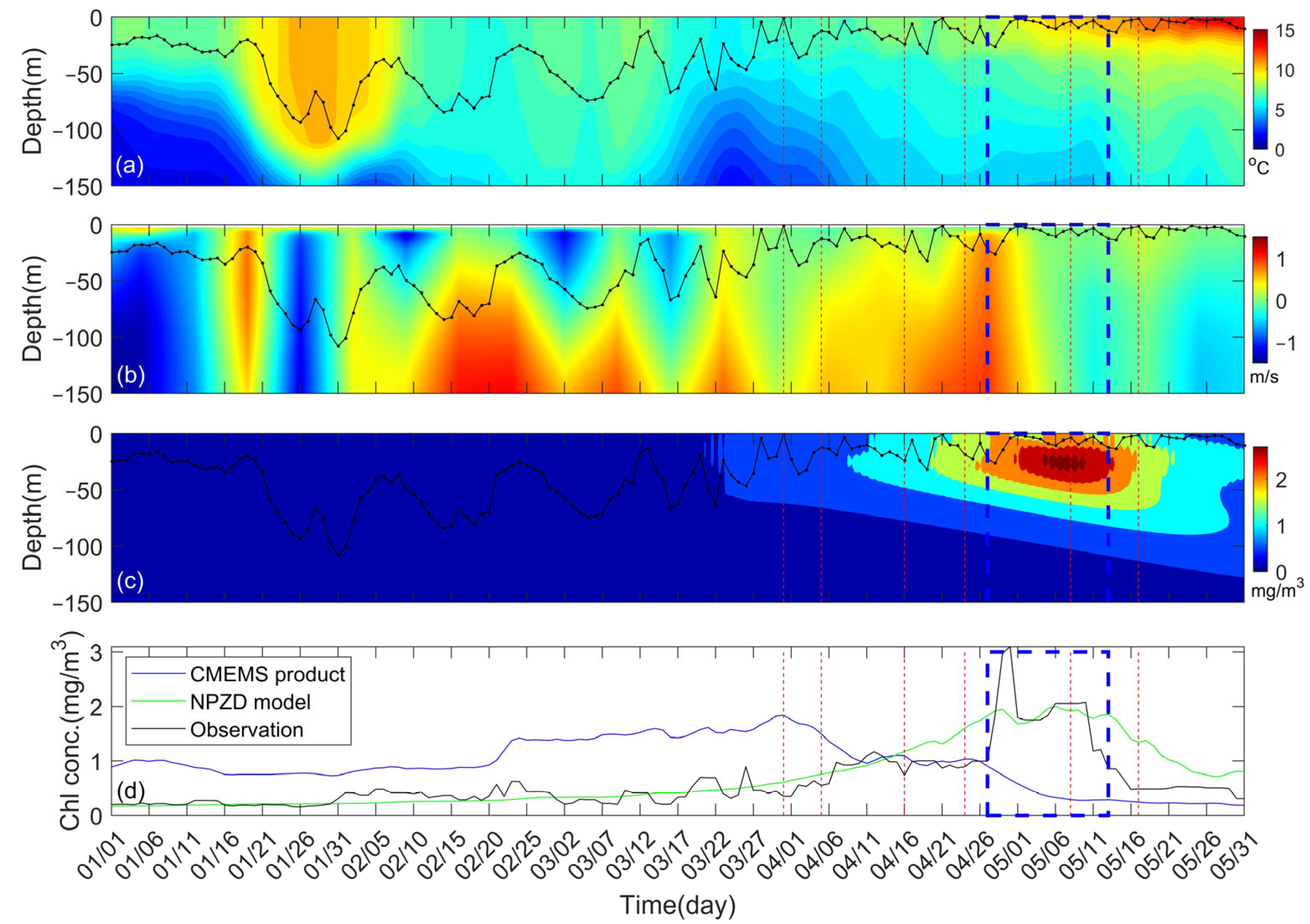
3.1. Secondary Bloom Observations

In addition to typical blooms in spring and autumn in the EJS, we found a secondary bloom followed by a spring bloom. Both the GOCI observations and CMEMS reanalysis data showed similar temporal and spatial Chla distributions near eddy ED. In Figure 2, the mean Chla concentration over EJS (rectangular domain in Figure 1) shows that the spring bloom strengthened in early March and decayed in early May when the water surface temperature reached 7 °C, beyond which the bloom began to decline due to thermal stress on the phytoplankton. The autumn bloom from October to November was found to have a much weaker Chla concentration than that in the spring bloom (blue line in Figure 2). Focusing on the area on eddy ED, a short and intense bloom (hereafter referred to as a secondary bloom) occurred in the eddy interior over the course of the weakening spring bloom (red line in Figure 2).
Snapshots of the Chla distribution in the proximity of eddy ED showed a few temporal phases of Chla distribution (Figure 3). Chla-depleted regions were observed inside and outside the eddy before the spring bloom began (Figure 3a). From this time to the peak of the spring bloom, a high contrast in the Chla concentration with weaker Chla inside the eddy was observed (Figure 3b–d). At the spring bloom peak, the formation of Chla-rich submesoscale filaments with relatively weaker Chla concentrations inside the eddy was observed (Figure 3f). As the spring bloom declined, a high contrast in Chla concentration with Chla-rich filaments inside the eddy was observed (secondary bloom shown in Figure 3h). At the end of May, following the secondary bloom, the Chla was depleted over the EJS.

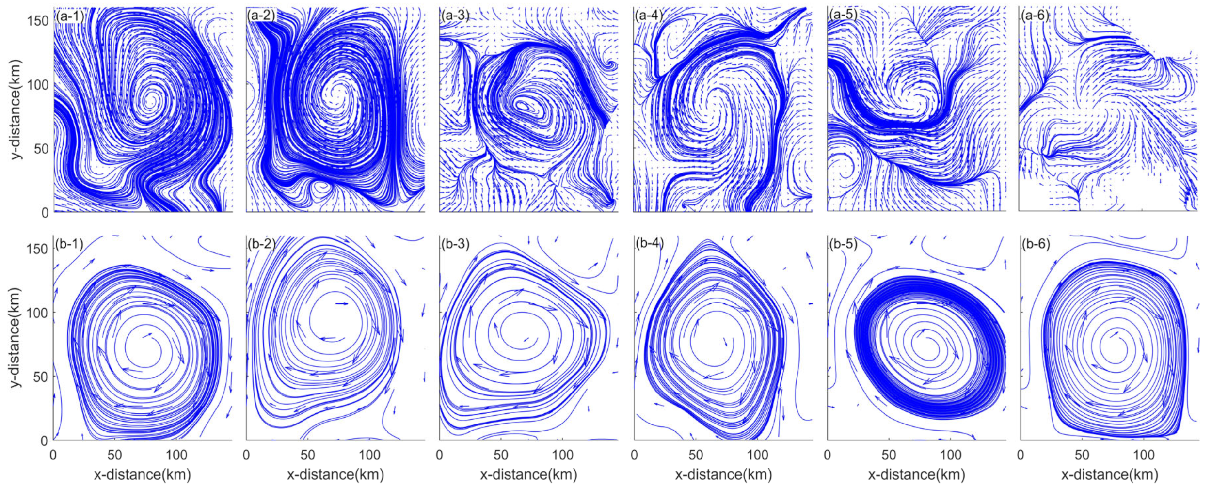
3.2. Current Observations

The flow kinematics near eddy ED were compared using two satellite-based Eulerian currents, namely the mesoscale-permitting AVISO geostrophic current and the submesoscale-permitting GOCI surface current, to stress the importance of high-resolution Eulerian velocity observations in elucidating physical–biological interaction mechanisms. Figure 4 depicts GOCI velocity fields with a 5 km grid and AVISO velocity fields with a 25 km grid over the period of the spring and secondary blooms. The speed of the GOCI current in an eddy-centric coordinate increased and then decreased in the radial direction from the core to its circumference, so the eddy showed a Rankine-type vortex motion, where it attained a maximum speed in the space between the center and edge. If the eddy boundaries observed in the GOCI currents were applied to the AVISO currents, the speed of the AVISO current would increase in the radial direction from the eddy core to its circumference, showing a rigid body rotational motion.
Figure 5 shows the streamlines, defined as a path of massless imaginary water particles traveling along lines that are tangential to the local Eulerian velocity. The GOCI current shows intense spiral streamlines in the eddy during the early stage of the spring bloom (Figure 5(a1,a2)). This observation implies that water particles at the eddy core must take a long path to escape from the eddy. In other words, intense spirals in a clockwise direction reveal a thicker material barrier between the inside and outside of the eddy, which also means that the horizontal transport and mixing of the material is limited by the material barriers. When the spring bloom declines, streamlines spiral outward in a clockwise direction (Figure 5(a4,a5)), which corresponds to the period of the secondary bloom. The outward spiral implies that the material barrier weakened, and horizontal transport and mixing were strengthened. We found that this coincided with the secondary bloom during the weakening spring bloom phase. The obvious temporal change in the streamlines seen in the GOCI currents was not identified by AVISO currents (Figure 5b).

3.3. Model Observations

Observational and model data at the time of the secondary bloom were investigated to estimate the physical processes related to the secondary bloom. The CMEMS model data suggested that the thickness of the mixed layer depth continued to decrease from March to May 2011 (black lines in Figure 6a,b), and the minimum mixed layer depth was reached in May when the secondary bloom occurred. The vertical velocity from the OMEGA3D model indicates a strong upwelling event at the end of April (Figure 6b); therefore, the modeled upwelling timing, and up to one week thereafter, matched well with the secondary bloom period. Therefore, various models and observations that can infer upwelling at the time of secondary bloom, such as the events of minimum mixed layer depth (model), strong positive vertical velocity (model), and streamlines spiraling outward (satellite observation), coincided with the time of the secondary bloom (satellite observation) from late April into early May.
Although the coincidence of the modeled positive vertical velocity and the observed secondary bloom appeared to indicate a physical–biological interaction, the GOBHM model (blue line in Figure 6d) was not able to predict the secondary bloom. This may be because the vertical fluctuations or upwelling of the mixed layer induced by submesoscale circulations cannot be simulated using the low-resolution model (0.25°), which also implies that the model did not detect the physical part of the physical–biological interaction needed to simulate the secondary bloom. Unlike the GOBHD model, we found that a simple one-dimensional NPZD model at eddy-centric coordinates could predict the secondary bloom almost simultaneously with the spring bloom (Figure 6c,d).

4. Discussion

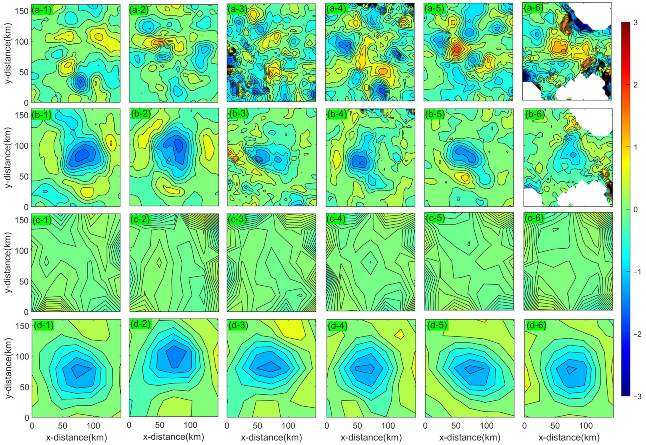
4.1. Divergence and Vorticity in a Mesoscale Eddy

During the spring bloom period, the GOCI current exhibited increasing horizontal divergence and decreasing horizontal vorticity; thus, strong divergence and weak vorticity were observed when the secondary bloom occurred (Figure 7(a1–a6,b1–b6)). Divergence measures the dilation rate and vorticity measures the rotation rate of a body of water. As seen in the outward streamlines in Figure 5, the divergence in the eddy interior became more pronounced with time (Figure 7(a1–a6)), reaching its peak on 8 May when the secondary bloom was noticed.
Unlike divergence, the vorticity in the eddy interior weakened slightly with time. The conservation of mass for incompressible flow implies that positive horizontal divergence is necessarily accompanied by positive vertical transport. Therefore, it is physically obvious that upwelling occurred in the eddy interior at the time of strong positive divergence, especially on 8 May, when the secondary bloom occurred. GOCI surface currents manifested variations in divergence and vorticity for the eddy; however, the variation was limited to extraction from the mesoscale-permitting AVISO geostrophic current (Figure 7(c1–c6,d1–d6)) because it excludes many current components in the submesoscale, including the Ekman current, wind drift, Stokes drift, ageostrophic current, and multiscale interactions between the components.

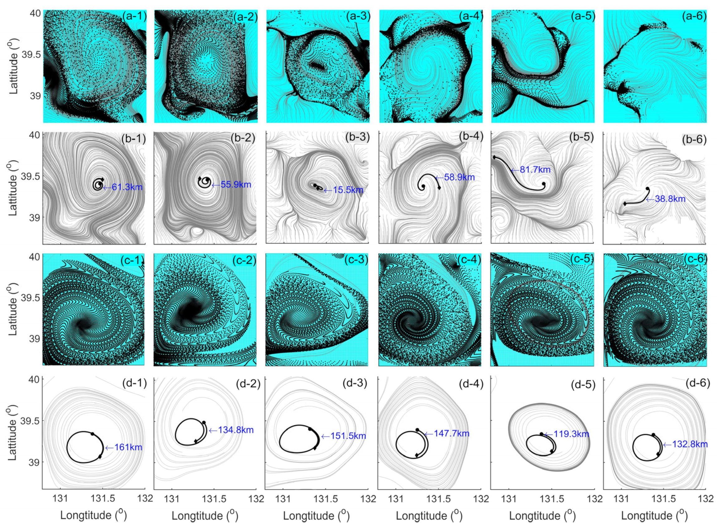
4.2. Horizontal Material Transport in a Mesoscale Eddy

The particle tracking model [45] driven by GOCI currents, visualizes the characteristics of horizontal transport in the spring and secondary bloom periods. The 20,164 particles were initially located in a regular grid spaced at 1 km and advected by a steady GOCI current for eight days. During the early phase of the spring bloom (Figure 8(a1,a2)), a large portion of the particles remained inside the eddy, and the eddy boundaries did not show a sharp convergence line. At the peak of the spring bloom (Figure 8(a3)), the particles were less populated inside the eddy, except for the eddy core, and a sharp convergence region appeared around the eddy. During the secondary bloom period (Figure 8(a4,a5)), the particles converged to the surrounding filament, with an even smaller population remaining inside the eddy. As expected, the GOCI current on 8 May produced the longest particle trajectory and greatest displacement among particles discharged from the eddy core. As expected, the smallest displacement of a particle discharged from the eddy core was observed during the early phase of the spring bloom period (Figure 8(b1–b3)). The GOCI current on 8 May produced the longest particle trajectory and greatest displacement event among those discharged from the eddy core (Figure 8(b5)). Particle simulations utilizing AVISO currents lacked the temporal and spatial variability observed in GOCI currents, resulting in a homogeneous particle distribution in the eddy interior for all simulation cases Figure 8(c1–c6,d1–d6).

4.3. Possible Bloom Mechanisms

Mesoscale eddies influence secondary Chla blooms through various mechanisms of physical–biological interactions, such as eddy stirring [46], eddy trapping [47], eddy pumping [48], and eddy–wind interaction [49]. Eddy stirring describes the spatial variation of the Chla anomaly in the eddy that propagates with a large-scale current, which is not applicable to eddy ED, since it remained stationary for a year. Eddy trapping occurs when an eddy is snatched away from the mainstream, resulting in nutrient-poor, trapped eddy interiors that quickly deplete the Chla concentration inside the eddy. Eddy ED, during the early phase of the spring bloom, seemingly underwent eddy trapping, because the limited horizontal transport shown from the particle tracking model can also limit vertical transport by considering mass conservation. Consequently, eddy stirring and eddy trapping associated with horizontal transport were not regarded as triggers for secondary blooms.
Eddy pumping and eddy–wind interactions are linked to vertical transport, which can directly alter the nutrition and light availability in the surface layer, thereby possibly explaining the secondary bloom we observed. Eddy pumping is the vertical undulation of the isopycnal that pumps nutrients up or down, and pumping through the bottom of the mixed layer is connected to eddy evolution, including intensification or relaxation. For anticyclonic eddies in the northern hemisphere, upwelling occurs during eddy intensification, and downwelling occurs during eddy relaxation [7]. By measuring temporal changes in vorticity, we can determine whether an eddy intensifies or relaxes. The conservation of angular momentum indicates that the vorticity of a vortex can increase as its vertical extent thickens (vortex stretching) and decrease as its vertical extent thins (vortex squeezing) [50]. Vortex stretching and vortex squeezing are defined as moments of mixed layer thickening and thinning, respectively, in our application. Because the vorticity at the eddy core decreased as the mixed layer depth decreased towards the time of secondary bloom, eddy ED was possibly in the phase of relaxation or decay during the spring bloom period. Eddy–wind interaction, also known as Ekman suction (upwelling) or Ekman pumping (downwelling), is the interaction between winds and ocean surface currents that can result in vertical velocity changes at the bottom of the Ekman layer. Although the AVISO current was not able to manifest the temporal variations in divergence and vorticity that can be shown by GOCI currents, it manifested a wind–eddy-induced positive vertical velocity that roughly matched the Chla peaks observed during the secondary bloom (Figure 9).
From the arguments above, we consider that eddy trapping, eddy pumping, and eddy–wind interaction are possible mechanisms underlying the variation in Chla concentration during the observed spring and secondary blooms. The interior of the eddy was trapped, as indicated by the intense streamlines (Figure 5), and particles were widely distributed inside the eddy (Figure 8). This eddy trapping continued before the spring bloom peak, which resulted in a negative Chla anomaly because isolation in both the horizontal and vertical directions restricted the availability of nutrients. After this period, the isolation relaxed, as observed in the outward streamlines, along with particle depletion inside the eddy and strong divergence in the eddy interior. Eddy pumping continued until the end of the secondary bloom. During the eddy pumping period, the eddy–wind interaction played a role in enhancing the upwelling during the secondary bloom (Figure 9). Even though the NPZD model was not incorporated with the eddy–wind interaction, it estimated the secondary bloom at the right time. This suggests that eddy pumping triggered the secondary bloom, and the eddy–wind interaction created sharp Chla peaks around 28 April and 8 May (Figure 9).

5. Conclusions

Based on satellite observations, we investigated the mesoscale eddy dynamics and the corresponding Chla variation in the EJS to investigate the physical–biological interactions involved in the secondary bloom that occurred in the decaying phase of the spring bloom. When the secondary bloom occurred, we observed streamlines spiraling outward with stronger divergence and weaker vorticity, which also coincided with the modeled upwelling and shallowest mixed layer depth. This strongly suggests that the secondary bloom was triggered by upwelling, which may modulate nutrient and light availability in the surface layer.
The mechanisms of eddy trapping, eddy pumping, and eddy–wind interactions were considered to involve the Chla variations observed during the spring bloom period. The interior region of the eddy was trapped (eddy trapping) during the early spring bloom, as indicated by strong material barriers surrounding the eddy, which may have led to a scarcity of nutrients, and ultimately Chla depletion within the eddy. Then, the divergence and vorticity within the eddy first increased and then decreased as the mixed layer thinned, which implies that the eddy was in the phase of relaxation with upwelling (eddy pumping). This upwelling corresponded to a secondary bloom. We discovered a sharp Chla peak that was consistent with substantial Ekman suction (eddy–wind interaction); consequently, eddy–wind interaction may have stimulated the bloom on a shorter timescale than did eddy pumping.
Submesoscale observations of surface currents reveal the hidden physical dynamics that play an important role in the physical–biological interaction. In this study, we observed the first satellite observation of surface layer divergence inside a mesoscale eddy with internal Chla blooms in the East/Japan Sea using the submesoscale-permitting GOCI-based surface current. This Eulerian observation is limited to any other Eulerian observational current that can cover the region of mesoscale eddies because it is incapable of resolving the submesoscale in both time and space. Even a linear combination of the wind and the AVISO current may not be able to replicate the submesoscale currents that we were able to make using the GOCI Chla data. Submesoscale circulations, such as filaments, eddies, and fronts, are nonlinear phenomena that are closely related to vertical transport (upwelling and downwelling). These vertical transports are an order of magnitude stronger than those caused by mesoscale phenomena, and the spatiotemporal scales of wind are much larger than those of upwelling caused by submesoscale circulations. Consequently, the wind contribution may not cause appreciable changes in surface layer divergence. This work stresses the importance of high-resolution velocity fields in investigating the physical mechanism of the physical–biological interaction, and a long-term and high-resolution Eulerian observation platform that can span a marginal sea is required to study the long-term interaction between mesoscale eddies and variations in Chla production.

Author Contributions

Conceptualization, J.M.C.; Methodology, T.T.M.H.; Software, T.T.M.H.; Validation, J.M.C. and T.T.M.H.; Formal Analysis, J.M.C.; Investigation, J.M.C.; Resources, T.T.M.H.; Data Curation; Writing—Original Draft Preparation, J.M.C.; Writing—Review and Editing, Y.-G.P.; Visualization, T.T.M.H.; Supervision, J.M.C.; Project Administration, Y.-G.P.; Funding Acquisition, Y.-G.P. All authors have read and agreed to the published version of the manuscript.

Funding

This work was supported by the National Research Foundation of Korea (NRF) grant funded by the Korea government (MSIT) (no. 2022R1C1C1011747) and the Ministry of Oceans and Fisheries, South Korea (Investigation and prediction system development of marine heatwave around the Korean Peninsula originated from the subarctic and Western Pacific (20190344)). This research was also supported by Korea Institute of Marine Science & Technology Promotion(KIMST) funded by the Ministry of Oceans and Fisheries, Korea (20180447, Improvements of ocean prediction accuracy using numerical modeling and artificial intelligence technology).

Data Availability Statement

Not applicable.

Conflicts of Interest

The authors declare no conflict of interest.

References

  1. Ferrari, R.; Wunsch, C. Ocean circulation kinetic energy: Reservoirs, sources, and sinks. Annu. Rev. Fluid Mech. 2009, 41, 253–282. [Google Scholar] [CrossRef]
  2. Kim, D.; Yang, E.J.; Kim, K.H.; Shin, C.W.; Park, J.; Yoo, S.; Hyun, J.H. Impact of an anticyclonic eddy on the summer nutrient and chlorophyll a distributions in the Ulleung Basin, East Sea (Japan Sea). ICES J. Mar. Sci. 2012, 69, 23–29. [Google Scholar] [CrossRef]
  3. Arostegui, M.C.; Gaube, P.; Woodworth Jefcoats, P.A.; Kobayashi, D.R.; Braun, C.D. Anticyclonic eddies eggreagate pelagic predators in a subtropical gyre. Nature 2022, 609, 535–540. [Google Scholar] [CrossRef] [PubMed]
  4. Ma, Z.; Fei, J.; Liu, L.; Huang, X.; Li, Y. An investigation of the influences of mesoscale ocean eddies on tropical cyclone intensities. Mon. Weather Rev. 2017, 145, 1181–1201. [Google Scholar] [CrossRef]
  5. Small, R.J.; Msadek, R.; Kwon, Y.O.; Booth, J.F.; Zarzycki, C. Atmosphere surface storm track response to resolved ocean mesoscale in two sets of global climate model experiments. Clim. Dyn. 2019, 52, 2067–2089. [Google Scholar] [CrossRef]
  6. Korotenko, K.A. Effects of mesoscale eddies on behavior of an oil spill resulting from an accidental deepwater blowout in the Black Sea: An assessment of the environmental impacts. PeerJ 2018, 6, e5448. [Google Scholar] [CrossRef]
  7. McGillicuddy, D.J., Jr. Mechanisms of physical-biological-biogeochemical interaction at the oceanic mesoscale. Annu. Rev. Mar. Sci. 2016, 8, 125–159. [Google Scholar] [CrossRef]
  8. Chen, Y.; Tang, D. Eddy-feature phytoplankton bloom induced by a tropical cyclone in the South China Sea. Int. J. Remote Sens. 2012, 33, 7444–7457. [Google Scholar] [CrossRef]
  9. Ciancia, E.; Lacava, T.; Pergola, N.; Vellucci, V.; Antoine, D.; Satriano, V.; Tramutoli, V. Quantifying the Variability of Phytoplankton Blooms in the NW Mediterranean Sea with the Robust Satellite Techniques (RST). Remote Sens. 2021, 13, 5151. [Google Scholar] [CrossRef]
  10. Korotenko, K.; Osadchiev, A.; Melnikov, V. Mesoscale Eddies in the Black Sea and Their Impact on River Plumes: Numerical Modeling and Satellite Observations. Remote Sens. 2022, 14, 4149. [Google Scholar] [CrossRef]
  11. McGillicuddy, D.J., Jr.; Kosnyrev, V.K.; Ryan, J.P.; Yoder, J.A. Covariation of mesoscale ocean color and sea-surface temperature patterns in the Sargasso Sea. Deep Sea Res. Part II Top. Stud. Oceanogr. 2001, 48, 1823–1836. [Google Scholar] [CrossRef]
  12. Dong, C.; Liu, L.; Nencioli, F.; Bethel, B.J.; Liu, Y.; Xu, G.; Ma, J.; Ji, J.; Sun, W.; Shan, H.; et al. The near-global ocean mesoscale eddy atmospheric-oceanic-biological interaction observational dataset. Sci. Data 2022, 9, 436. [Google Scholar] [CrossRef]
  13. Zhu, Y.; Liang, X. Characteristics of Eulerian Mesoscale Eddies in the Gulf of Mexico. Front. Mar. Sci. 2022, 9, 2655. [Google Scholar] [CrossRef]
  14. Shi, Y.; Liu, X.; Liu, T.; Chen, D. Characteristics of Mesoscale Eddies in the Vicinity of the Kuroshio: Statistics from Satellite Altimeter Observations and OFES Reanalysis Data. J. Mar. Sci. Eng. 2022, 10, 1975. [Google Scholar] [CrossRef]
  15. Mkhinini, N.; Coimbra, A.L.S.; Stegner, A.; Arsouze, T.; Taupier-Letage, I.; Béranger, K. Long-lived mesoscale eddies in the eastern Mediterranean Sea: Analysis of 20 years of AVISO geostrophic velocities. J. Geophys. Res. Ocean. 2014, 119, 8603–8626. [Google Scholar] [CrossRef]
  16. Ioannou, A.; Stegner, A.; Tuel, A.; LeVu, B.; Dumas, F.; Speich, S. Cyclostrophic corrections of AVISO/DUACS surface velocities and its application to mesoscale eddies in the Mediterranean Sea. J. Geophys. Res. Ocean. 2019, 124, 8913–8932. [Google Scholar] [CrossRef]
  17. Kurczyn, J.A.; Beier, E.; Lavín, M.F.; Chaigneau, A. Mesoscale eddies in the northeastern Pacific tropical-subtropical transition zone: Statistical characterization from satellite altimetry. J. Geophys. Res. Ocean. 2012, 117, C10021. [Google Scholar] [CrossRef]
  18. Kang, J.J.; Jang, H.K.; Lim, J.H.; Lee, D.; Lee, J.H.; Bae, H.; Lee, C.H.; Kang, C.-K.; Lee, S.H. Characteristics of Different Size Phytoplankton for Primary Production and Biochemical Compositions in the Western East/Japan Sea. Front. Microbiol. 2020, 11, 560102. [Google Scholar] [CrossRef]
  19. Choi, J.; Park, Y.G.; Kim, W.; Kim, Y.H. Characterization of submesoscale turbulence in the east/japan sea using geostationary ocean color satellite images. Geophys. Res. Lett. 2019, 46, 8214–8223. [Google Scholar] [CrossRef]
  20. George, J.V.; Nuncio, M.; Chacko, R.; Anilkumar, N.; Noronha, S.B.; Patil, S.M.; Pavithran, S.; Alappattu, D.P.; Krishnan, K.P.; Achuthankutty, C.T. Role of physical processes in chlorophyll distribution in the western tropical Indian Ocean. J. Mar. Syst. 2013, 113, 1–12. [Google Scholar] [CrossRef]
  21. McWilliams, J.C. Submesoscale currents in the ocean. Proc. R. Soc. A Math. Phys. Eng. Sci. 2016, 472, 20160117. [Google Scholar] [CrossRef] [PubMed]
  22. Berta, M.; Griffa, A.; Haza, A.C.; Horstmann, J.; Huntley, H.S.; Ibrahim, R.; Lund, B.; Özgökmen, T.M.; Poje, A.C. Submesoscale kinematic properties in summer and winter surface flows in the Northern Gulf of Mexico. J. Geophys. Res. Ocean. 2020, 125, e2020JC016085. [Google Scholar] [CrossRef]
  23. Liu, G.; Bracco, A.; Sitar, A. Submesoscale Mixing Across the Mixed Layer in the Gulf of Mexico. Front. Mar. Sci. 2021, 8, 615066. [Google Scholar] [CrossRef]
  24. Kim, W.; Moon, J.E.; Park, Y.J.; Ishizaka, J. Evaluation of chlorophyll retrievals from Geostationary Ocean color imager (GOCI) for the north-east Asian region. Remote Sens. Environ. 2016, 184, 482–495. [Google Scholar] [CrossRef]
  25. Park, M.S.; Lee, S.; Ahn, J.H.; Lee, S.J.; Choi, J.K.; Ryu, J.H. Decadal Measurements of the First Geostationary Ocean Color Satellite (GOCI) Compared with MODIS and VIIRS Data. Remote Sens. 2021, 14, 72. [Google Scholar] [CrossRef]
  26. Park, K.A.; Park, J.E.; Kang, C.K. Satellite-Observed Chlorophyll-a Concentration Variability in the East Sea (Japan Sea): Seasonal Cycle, Long-Term Trend, and Response to Climate Index. Front. Mar. Sci. 2022, 9, 807570. [Google Scholar] [CrossRef]
  27. Yamada, K.; Ishizaka, J.; Yoo, S.; Kim, H.C.; Chiba, S. Seasonal and interannual variability of sea surface chlorophyll a concentration in the Japan/East Sea (JES). Prog. Oceanogr. 2004, 61, 193–211. [Google Scholar] [CrossRef]
  28. Chen, S.; Meng, Y.; Lin, S.; Xi, J. Remote Sensing of the Seasonal and Interannual Variability of Surface Chlorophyll-a Concentration in the Northwest Pacific over the Past 23 Years (1997–2020). Remote Sens. 2022, 14, 5611. [Google Scholar] [CrossRef]
  29. Ashijan, C.; Arnone, R.A.; Davis, C.; Jones, B.; Kahru, M.; Lee, C.; Mitchell, B.G. Biological Structure and Seasonality in the Japan/East Sea. Oceanography 2006, 19, 122–133. [Google Scholar] [CrossRef]
  30. Faghmous, J.H.; Frenger, I.; Yao, Y.; Warmka, R.; Lindell, A.; Kumar, V. A daily global mesoscale ocean eddy dataset from satellite altimetry. Sci. Data 2015, 2, 150028. [Google Scholar] [CrossRef] [Green Version]
  31. Emery, W.J.; Thomas, A.C.; Collins, M.J.; Crawford, W.R.; Mackas, D.L. An objective procedure to compute advection from sequential infrared satellite images. J. Geophys. Res. 1986, 91, 12–865. [Google Scholar]
  32. Zavialov, P.O.; Grigorieva, J.V.; Möller, O.O., Jr.; Kostianoy, A.G.; Gregoire, M. Continuity preserving modified maximum cross-correlation technique. J. Geophys. Res. Ocean. 2002, 107, 24-1. [Google Scholar] [CrossRef]
  33. Yang, H.; Choi, J.K.; Park, Y.J.; Han, H.J.; Ryu, J.H. Application of the Geostationary Ocean Color Imager (GOCI) to estimates of ocean surface currents. J. Geophys. Res. Ocean. 2014, 119, 3988–4000. [Google Scholar] [CrossRef]
  34. Yang, H.; Arnone, R.; Jolliff, J. Estimating advective near-surface currents from ocean color satellite images. Remote Sens. Environ. 2015, 158, 1–14. [Google Scholar] [CrossRef]
  35. Park, J.E.; Park, K.A.; Ullman, D.S.; Cornillon, P.C.; Park, Y.J. Observation of diurnal variations in mesoscale eddy sea-surface currents using GOCI data. Remote Sens. Lett. 2016, 7, 1131–1140. [Google Scholar] [CrossRef]
  36. Sun, H.; Song, Q.; Shao, R.; Schlicke, T. Estimation of sea surface currents based on ocean colour remote-sensing image analysis. Int. J. Remote Sens. 2016, 37, 5105–5121. [Google Scholar] [CrossRef]
  37. Warren, M.A.; Quartly, G.D.; Shutler, J.D.; Miller, P.I.; Yoshikawa, Y. Estimation of ocean surface currents from maximum cross correlation applied to GOCI geostationary satellite remote sensing data over the Tsushima (Korea) Straits. J. Geophys. Res. Ocean. 2016, 121, 6993–7009. [Google Scholar] [CrossRef]
  38. Liu, J.; Emery, W.J.; Wu, X.; Li, M.; Li, C.; Zhang, L. Computing ocean surface currents from GOCI ocean color satellite imagery. IEEE Trans. Geosci. Remote Sens. 2017, 55, 7113–7125. [Google Scholar] [CrossRef]
  39. Choi, J.M.; Kim, W.; Hong, T.T.M.; Park, Y.G. Derivation and Evaluation of Satellite-Based Surface Current. Front. Mar. Sci. 2021, 8, 695780. [Google Scholar] [CrossRef]
  40. Thielicke, W.; Stamhuis, E. PIVlab–towards user-friendly, affordable and accurate digital particle image velocimetry in MATLAB. J. Open Res. Softw. 2014, 2. [Google Scholar] [CrossRef]
  41. Mason, E.; Pascual, A.; McWilliams, J.C. A new sea surface height–based code for oceanic mesoscale eddy tracking. J. Atmos. Ocean. Technol. 2014, 31, 1181–1188. [Google Scholar] [CrossRef] [Green Version]
  42. Delepoulle, A.; Chelton, D.; Schlax, M.; Faugere, Y.; Dibarboure, G. 24 year mesoscale eddy trajectory atlas on AVISO. In Geophysical Research Abstracts; EGU2018-13690; European Geosciences Union: Vienna, Austria, 2018; Volume 20. [Google Scholar]
  43. Kuhn, A.M.; Fennel, K.; Mattern, J.P. Model investigations of the North Atlantic spring bloom initiation. Prog. Oceanogr. 2015, 138, 176–193. [Google Scholar] [CrossRef]
  44. Li, J.; Qi, Y.; Jing, Z.; Wang, J. Enhancement of eddy-Ekman pumping inside anticyclonic eddies with wind-parallel extension: Satellite observations and numerical studies in the South China Sea. J. Mar. Syst. 2014, 132, 150–161. [Google Scholar] [CrossRef]
  45. Jalón-Rojas, I.; Wang, X.H.; Fredj, E. A 3D numerical model to track marine plastic debris (TrackMPD): Sensitivity of microplastic trajectories and fates to particle dynamical properties and physical processes. Mar. Pollut. Bull. 2019, 141, 256–272. [Google Scholar] [CrossRef]
  46. Martin, A.P. Phytoplankton patchiness: The role of lateral stirring and mixing. Prog. Oceanogr. 2003, 57, 125–174. [Google Scholar] [CrossRef]
  47. D’Ovidio, F.; De Monte, S.; Della Penna, A.; Cotté, C.; Guinet, C. Ecological implications of eddy retention in the open ocean: A Lagrangian approach. J. Phys. A Math. Theor. 2013, 46, 254023. [Google Scholar] [CrossRef]
  48. Gaube, P.; McGillicuddy, D.J., Jr.; Chelton, D.B.; Behrenfeld, M.J.; Strutton, P.G. Regional variations in the influence of mesoscale eddies on near-surface chlorophyll. J. Geophys. Res. Ocean. 2014, 119, 8195–8220. [Google Scholar] [CrossRef] [Green Version]
  49. Stern, M.E. Interaction of a uniform wind stress with a geostrophic vortex. In Deep Sea Research and Oceanographic Abstracts; Elsevier: Amsterdam, The Netherlands, 1965; Volume 12, pp. 355–367. [Google Scholar]
  50. Tennekes, H.; Lumley, J.L. A First Course in Turbulence; The Massachusetts Institute of Technology: NewYork, NY, USA, 1972; Chapter 2; Volume 9. [Google Scholar]
Figure 1. GOCI Chla concentration at 3 a.m. UTC on 3/31/2011 (a) and at 2 a.m. UTC on 5/8/2011 (b) in EJS. The red point indicates the location of eddy ED.
Remotesensing 15 00995 g001
Figure 2. The temporal distribution of mean Chla concentrations in 2011. The solid and dashed blue lines represent the mean Chla concentrations and sea surface temperatures over the EJS (rectangular domain in Figure 1) derived from CMEMS products. The solid and dashed red lines are the mean Chla concentrations and sea surface temperatures at the center of eddy ED on 5/8 derived from the CMEMS products. The black points represent mean Chla concentrations derived from GOCI data.
Remotesensing 15 00995 g002
Figure 3. CMEMS Chla reanalysis data with a horizontal resolution of 4 km near eddy ED on 3/1 (a), 3/10 (b), 3/20 (c), 3/31 (d), 4/5 (e), 4/16 (f), 4/24 (g), 5/8 (h), 5/17 (i), and 5/31 (j).
Remotesensing 15 00995 g003
Figure 4. GOCI velocity fields with a 5 km grid (a1a6) and AVISO velocity fields with a 25 km grid (b1b6) during the period of the spring and secondary blooms, taken on 3/31, 4/5, 4/16, 4/24, 5/8, 05/17. The color scale is the spatial and temporal Chla concentration on the same date as the velocity field over EJS.
Remotesensing 15 00995 g004
Figure 5. Streamlines from GOCI velocity fields with a grid of 5 km (a1a6) and AVISO velocity fields with a grid of 25 km (b1b6) over eddy ED on 3/31, 4/5, 4/16, 4/24, 5/8, and 5/17, respectively.
Remotesensing 15 00995 g005
Figure 6. (a) The temporal distribution of depth temperature at the center of eddy ED on 5/8. (b) Temporal distribution of vertical velocity in depth at the center of eddy ED on 5/8. (c) The temporal Chla concentration with depth from the NPZD model on 05/08. (d) Temporal Chla concentration at the surface of eddy ED on 5/8 from the NPZD model (green line), CMEMS product (blue line), and observation from satellite (black line). The blue box defines the bloom period (4/27–5/12). The dashed red lines indicate the dates of observation derived from GOCI data (3/31, 4/5, 4/16, 4/24, 5/8, and 5/17). The point black line is the mix layer depth at the center of eddy ED on 5/8 from January to May of 2011.
Remotesensing 15 00995 g006
Figure 7. Divergence (a1a6) and vorticity (b1b6) of eddy ED from GOCI data with a resolution of 5 km over the eddy ED. Divergence (c1c6) and vorticity (d1d6) of eddy ED from AVISO data with a resolution of 25 km over eddy ED. Indices 1–6 correspond to the days of 3/31, 4/5, 4/16, 4/24, 5/8, and 5/17, respectively.
Remotesensing 15 00995 g007
Figure 8. Distribution of 20,164 virtual particles in and around eddy ED after eight days for GOCI currents (a1a6) and AVISO currents (c1c6). The length of trajectory of the particle from the center of eddy from the initial point to the final point for GOCI currents (b1b6) and AVISO currents (d1d6). The cyan points are the initial position of particles. The black points are the final location of particles. The gray lines are the streamlines from the GOCI velocity field. The indices 1–6 represent the days 3/31, 4/5, 4/16, 4/24, 5/8, and 5/17, respectively.
Remotesensing 15 00995 g008
Figure 9. Temporal change in Ekman pumping velocity of the secondary bloom in January–May 2011. The solid pink line is the Ekman pumping velocity calculated from AVISO and wind data. The diamond points are the Ekman pumping velocity calculated from GOCI and wind data. The green line represents the temporal Chla concentration derived from the NPZD model. The blue box defines the bloom period (4/27–5/12). The dashed red lines indicate the days with observations from GOCI data (3/31, 4/5, 4/16, 4/24, 5/8, and 5/17).
Remotesensing 15 00995 g009
Disclaimer/Publisher’s Note: The statements, opinions and data contained in all publications are solely those of the individual author(s) and contributor(s) and not of MDPI and/or the editor(s). MDPI and/or the editor(s) disclaim responsibility for any injury to people or property resulting from any ideas, methods, instructions or products referred to in the content.

