Mapping Vegetation Index-Derived Actual Evapotranspiration across Croplands Using the Google Earth Engine Platform

Abstract

Precise knowledge of crop water consumption is essential to better manage agricultural water use, particularly in regions where most countries struggle with increasing water and food insecurity. Approaches such as cloud computing and remote sensing (RS) have facilitated access, process, and visualization of big geospatial data to map and monitor crop water requirements. To find the most reliable Vegetation Index (VI)-based evapotranspiration (ETa) for croplands in drylands, we modeled and mapped ETa using empirical RS methods across the Zayandehrud river basin in Iran for two decades (2000–2019) on the Google Earth Engine platform using the Normalized Difference Vegetation Index (NDVI) and the Enhanced Vegetation Index 2 (EVI2). Developed ET-VI products in this study comprise three NDVI-based ETa (ET-NDVI*, ET-NDVI*_scaled, and ET-NDVI_Kc) and an EVI2-based ETa (ET-EVI2). We (a) applied, for the first time, the ET-NDVI* method to croplands as a crop-independent index and then compared its performance with the ET-EVI2 and crop ET, and (b) assessed the ease and feasibility of the transferability of these methods to other regions. Comparing four ET-VI products showed that annual ET-EVI2 and ET-NDVI*_scaled estimations were close. ET-NDVI_Kc consistently overestimated ETa. Our findings indicate that ET-EVI2 and ET-NDVI_Kc were easy to parametrize and adopt to other regions, while ET-NDVI* and ET-NDVI*_scaled are site-dependent and sensitive to image acquisition time. ET-EVI2 performed robustly in arid and semi-arid regions making it a better tool. Future research should further develop and confirm these findings by characterizing the accuracy of VI-based ETa over croplands in drylands by comparing them with available ETa products and examining their performance using crop-specific comparisons.

1. Introduction

Water stress is significantly increasing in many countries in arid and semi-arid regions due to a sharp decline in precipitation. Consequently, these countries are not able to meet their water and food demands [1] and their agricultural sector is under severe pressure. The effect of drought on cultivated areas is a reduction of available water for actual evapotranspiration (ETa) and is often combined with increasing potential evapotranspiration that results in failing and declining crop yields [2]. This is because less water is available for irrigation when the demand is high. Agricultural areas are far more affected by water shortage than uncultivated land cover areas [3]. Thus, the accurate prediction of ETa, as the main indicator of crop water consumption, is essential for drought monitoring, irrigation scheduling, and sustainable water resources management [4,5].

Mapping the spatial distribution of ETa has been facilitated through remote sensing (RS) over large areas [6]. With the rise of cloud-based computing, the use of RS in many studies has greatly improved. Without the need to download and store data locally, a cloud-based platform such as Google Earth Engine (GEE) could effectively overcome the difficulties involved in large data processing and enable long-term environmental monitoring [7]. Using cloud computing platforms, researchers can share their scientific findings on a number of themes, including the monitoring of vegetation and crop water requirements, i.e., ETa at various spatial scales.

RS-based methods of ETa estimation can be classified into two groups: (1) satellite land surface temperature methods [8,9,10] and (2) vegetation index-based methods (ET-VI) [11,12,13]. In the first method, ETa is calculated as a residual of the energy balance equations using a thermal band collected from satellites [8,14], a variety of empirical and physically based models, input data, and assumptions to solve the energy balance equation [15]; while the link between crop coefficients (Kc) and reference ET (ETo) is employed in ET-VI-based approaches to predict crop water requirements [12,16].

The ET-VI method is one of the most commonly applied empirical approaches to model ETa using VIs as a proxy of Kc, as presented in the Food and Agriculture Organization (FAO56) method [14]. FAO56 applies the Penman–Monteith (PM) method to calculate the ET of a hypothetical reference crop, such as well-watered grass with a height of 12 cm, predefined roughness and albedo, and meteorological data [14]. Next, ETo is multiplied by Kc and Ks. Kc relates the ETa of a specific crop to those of the reference crop, while Ks describes the reduction of ETa due to water insufficiency. Under well-watered conditions (irrigation) Ks equals to 1 [14]. Similarly, in the ET-VI method, a VI is used to estimate the product of Kc and Ks [12,17]. Two Kc calculation approaches are considered in FAO56: (1) in most studies, Kc values are acquired using the single Kc approach which merges crop transpiration and soil evaporation into a single Kc coefficient [14,16,18], and less frequently, in method (2) the dual Kc approach is employed. This method determines crop transpiration and soil evaporation independently [18].

The most commonly used VIs are the Normalized Difference Vegetation Index (NDVI), Enhanced Vegetation Index (EVI), and the two-band version of the Enhanced Vegetation Index 2 (EVI2), which have been widely tested for ETa estimation in different landscapes including agricultural land [19,20,21,22,23], riparian vegetation [12,24,25,26], restored riparian [27], semi-arid sagebrush steppe [28], and urban green spaces [13,29,30]. Among these VIs, NDVI has been widely employed as a proxy of Kc at the field scale for different crops by determining the correlation between Kc and NDVI. The history of using NDVI as a proxy of Kc goes back to a study by Bausch and Neale (1987), who investigated the estimation of Kc using NDVI at two sites in Colorado; they validated the Kc estimated by radiometric measurements of NDVI against lysimeter measurements [31]. Kamble et al. (2013) developed a linear regression model between NDVI derived from MODerate Imaging Spectroradiometer (MODIS) and ground-based Kc extracted from AmeriFlux. A strong agreement was observed between the NDVI-Kc and the ground-based Kc during mid-season periods [32]. Duchemin et al. (2016) investigated the application of NDVI derived from Landsat 7 to estimate Kc values for wheat in Morocco, and reported a linear relationship between NDVI and Kc to monitor crop water requirements over irrigated agricultural fields [33]. The ability of NDVI to estimate ETa was examined using the Sentinel 2 and Venus satellites by French et al. (2020) over wheat fields at the farm scale in Yuma and Maricopa, Arizona, USA [23]. Comparisons of estimated ETa with crop evapotranspiration (ETc) observations revealed that RS-based ETa agreed well for most of the growing season, particularly during the mid-season [23]. Groeneveld et al. (2007) suggested the use of NDVI*, which reduces the scene-to-scene variability of Landsat images by removing NDVI outliers at the high- and low-ranges; their initial application estimated ETa over phreatophyte communities [34]. They scaled the NDVI by assigning values for bare soil at 0 and values for dense agricultural areas reflecting fully transpiring crops at 1.0 [35]. In this method, NDVI values are standardized between scene-specific bare soil NDVI (which means NDVI* equals to 0) and maximum NDVI (which means NDVI* equals to 1) to remove variation between scenes [34,36]. Bresloff et al. (2013) also applied these methods in desert phreatophyte communities after scaling sap flux measurements [37]. Jarchow et al. (2020) modified the Groeneveld equation and used NDVI* to calculate vegetation health and ETa dynamics in a semi-arid sagebrush steppe where ETa was calibrated with a 3-ha lysimeter [28], as well as for the ETa of tamarisk along the Shiprock, New Mexico, USA floodplain. Their seasonal ETa estimates for the New Mexico floodplain were significantly correlated with groundwater level (r² = 0.71) [38]. Recently, Nouri et al. (2020) applied EVI, EVI2, and NDVI* to estimate the ETa of urban green spaces where ET-EVI2 showed the highest correlation with ground data [39]. The NDVI* index has not been modified to be tested over croplands in an irrigation district per se. In a previous study, we evaluated the applicability of ET-VI for mapping and monitoring drought in arid agricultural systems using EVI and EVI2 and considering harvested area changes. We developed ET-EVI and ET-EVI2 using Landsat sensors over croplands in the Zayandehrud River Basin (ZRB) in Iran. Since EVI and EVI2 were optimized for MODIS and first used in estimating ETa [22], using these VIs with Landsat sensors required a cross-sensor transformation to allow for their use in the ET-VI algorithm (methodology can be found in [40]). Our results showed that ETa estimates agreed well with each other and are all suitable to monitor ETa in the ZRB. Compared to ETc values, ET-EVI2 performed slightly better across croplands.

This study aims to evaluate RS-based ET-VI methods over croplands by comparing the performance of four VIs – NDVI*, NDVI*_scaled, NDVI_Kc, and EVI2 – in the calculation of crop-independent ETa using reported ETc and FAO56 Kc values in the ZRB. In this study, we, for the first time: (a) applied NDVI* over croplands in a large irrigation district; and (b) assessed the applicability and possibilities of translation of these methods to other regions. Since over 40 different crops are cultivated in the ZRB and it is not possible to calibrate NDVIs as a proxy of Kc for all crops, we applied methods that are crop independent and suitable for operational applications. NDVI* ranges from 0 to 1 while the maximum Kc of many crops reaches 1.2 [41,42]. Therefore, NDVI* was scaled (NDVI*_scaled) to match the Kc range. NDVI_Kc is a crop-independent relationship between NDVI and Kc values described by [43]. We compared the ETa calculated using these three NDVIs to our localized ET-EVI2 [40], reported ETc derived from the local authorities’ reports, and crop-specific ET (wheat) values from the literature. The Google Earth Engine (GEE) platform was used to develop and generate ET-VIs and harvested areas’ changes time series in the ZRB.

The two main questions addressed in this paper are: (a) how to apply NDVI* to be adopted in agricultural lands for ETa estimation? So far, the application of NDVI* has not been tested for ETa estimation over croplands within basin-scale studies; therefore, we adjusted this index to be applied to crop water requirement estimation; and (b) which ET-VI is a better proxy of ETa over croplands? To find out which ET-VI performs better, ET-VIs were compared to reported ETa values. To evaluate the crop water requirements using ET-VIs time series, these methods were assessed in terms of ease of applicability and translation to other districts.

2. Materials and Methods

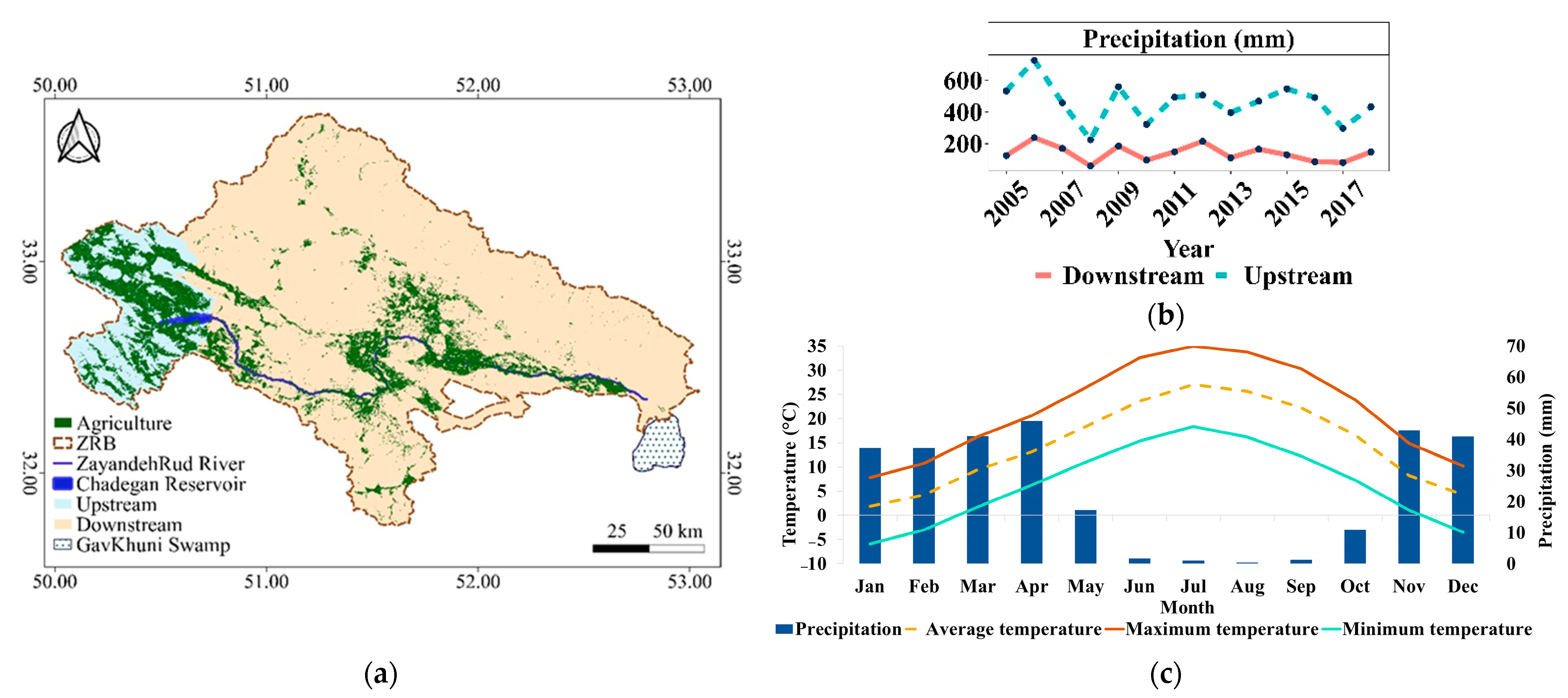
2.1. Study Site

One of the most important basins in central Iran is the ZRB which covers an area of 26,917 km² (Figure 1). The ZRB suffers from overexploitation, water scarcity, and recurring drought [44], and provides water for approximately 4.5 million residents [45]. The ZRB plays an important role in supplying potable, industrial, and agricultural water [46]. The main river of the basin flows 350 km [47] and is regulated by the Zayandehrud dam. Annual precipitation ranges from 63 mm downstream to 1281 mm upstream [40]. The average annual precipitation upstream is 475 mm and downstream is 144 mm (Figure 1b). The basin experiences the highest temperature from June to August (Figure 1c). Croplands are irrigated due to the low precipitation in the eastern and central parts of the basin. Wheat, barley, alfalfa, maize, potato, onion, and rice are the main staple crops of the basin [40]. Most farmlands in the ZRB are irrigated and the irrigation water is supplied by a dam. Drought and low rainfall result in less water release from the dam and consequently impairment of the agriculture sector and food production in the basin. Hence, analysis of spatial and temporal variations of ETa is vital to optimizing water resources management for irrigated agriculture.

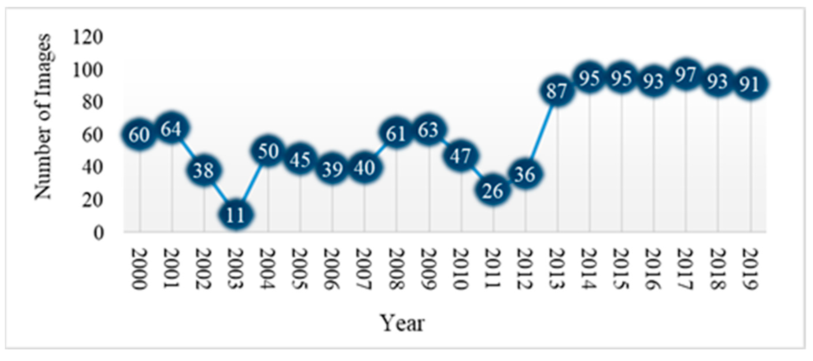
2.2. Satellite Data and Preprocessing

Landsat series (5 ETM, 7 ETM+, and 8 OLI) with a spatial resolution of 30 m for the period 2000–2019 were processed and corrected on the GEE platform to produce monthly VIs and ET-VIs time series (Figure 2). GEE consists of a repository of publicly accessible datasets, including satellite images from different sensors, and environmental, weather and climate, land cover, and topographic datasets with planetary-scale analysis capabilities [7,48]. It enabled us to process satellite images through a web-based code editor tool for algorithm development and accessing petabytes of data.

Corrected Landsat scenes for topography and bidirectional reflectance distribution function (BRDF) are further processed to remove clouds, shadows, snow, water, and poor-quality pixels. The missing data resulting from scan line errors in the Landsat 7 ETM+ were ignored, and we only retained data that was present. Abnormalities along the scene edges of Landsat 5 images were removed by applying a 500 m inwards-buffer mask. Discontinuity biases originating from small differences between the spectral characteristics of Landsat 5, 7, and 8 were addressed through transformation corrections developed by [49].

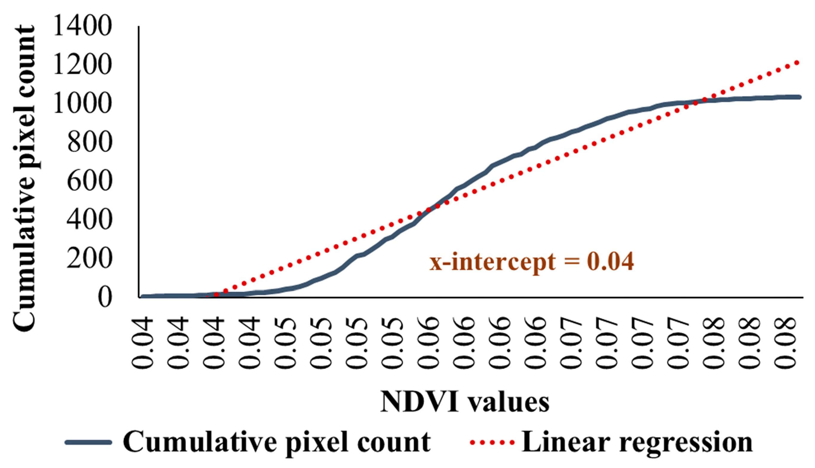
2.3. Calculation of NDVIs and ET-NDVIs

In this study, to calculate ET-NDVIs, three different NDVI-based proxies of Kc values were calculated: NDVI*, NDVI*_scaled, and NDVI_Kc. NDVI is a widely used index and proxy of vegetation health and greenness; it is calculated as a normalized ratio of the near-infrared (NIR) and red (R) bands:

$$\mathrm{NDVI}=\frac{\mathrm{NIR}-\mathrm{R}}{\mathrm{NIR}+\mathrm{R}}$$

(1)

NDVI* is an empirically modified version that aims to reduce the residual scene-to-scene variability of Landsat images by removing NDVI outliers at the high and low ends [28,38]. NDVI values were standardized between scene-specific bare soil (NDVI0) and most-active vegetation (NDVImax) to remove variation between scenes caused by atmospheric and soil conditions [34,36], and to compare scenes from different times under potentially different atmospheric opacities [34]. Groeneveld et al. (2007) identified NDVI0 inside homogeneous areas of native phreatophyte alkali scrub by using a simple linear regression over the lower portion of the cumulative frequency distribution for the pooled NDVI values for each year. We sampled constant areas with only bare soil inside each scene to calculate the mean NDVI0. For each image, NDVI0 was calculated using a simple linear regression of the cumulative frequency distribution applied to the sampled regions. The x-intercept resulting from the linear regression was chosen as the NDVI0 (Figure 3). To generate NDVImax, the absolute highest NDVI value was determined in each scene and then the average of all pixels falling within 5% of the maximum value was taken to be NDVImax [36,38,39,50]. NDVImax values vary scene-to-scene depending on absolute maximum values.

The NDVI* is then computed using the following equation:

$$\mathrm{NDVI}*=\frac{\mathrm{NDVI} - \mathrm{NDVI}0 }{\mathrm{NDVImax} - \mathrm{NDVI}0 }$$

(2)

According to FAO56, ETa is calculated as Ks × Kc × ETo. Consequently, VIs (NDVI*, NDVI*_scaled, and NDVI_Kc) are used to proxy the Ks × Kc value. Under unstressed and well-watered conditions, the maximum Kc of many crops reaches 1.2 [41,42] while NDVI cannot exceed 1. To use NDVI* as a proxy for Kc, we scaled NDVI* to match the Kc range and then compared NDVI* with NDVI*_scaled:

NDVI*_scaled = 1.2 × NDVI*

(3)

In the single Kc approach, the effect of crop transpiration and soil evaporation is incorporated into a single Kc that can be approximated with the NDVI. Many crops under unstressed conditions during the peak vegetation activity have a Kc of 1.2 [14] which approximately equals to an NDVI value of 0.8. Similar to that during the initial stage of the growing season, many crops have a Kc of 0.4 and an NDVI value of approximately 0.16 [18,43]. A crop-independent relationship between NDVI and Kc was reported by [18,41,43]:

NDVI_Kc = (1.25 × NDVI) + 0.2

(4)

Three versions of ETa were derived by multiplying pixel-wise estimated crop coefficients (NDVI_Kc, NDVI*, and NDVI*_scaled) and ETo values (Equations (5) – (7)).

ET-NDVI* = ETo × NDVI*

(5)

ET-NDVI*_scaled = ETo × NDVI*_scaled

(6)

ET-NDVI_Kc = ETo × NDVI_Kc

(7)

where ETo was calculated using GCWM. It should be noted that the VI method considers transpiration from green vegetation and only to a small extent the evaporation from bare soil. This explains possible underestimations during the initial and developing stages of the crop cycle [23].

After obtaining the ET-VI layers from GEE, missing monthly ET-VI values were replaced with average values from the previous and subsequent months.

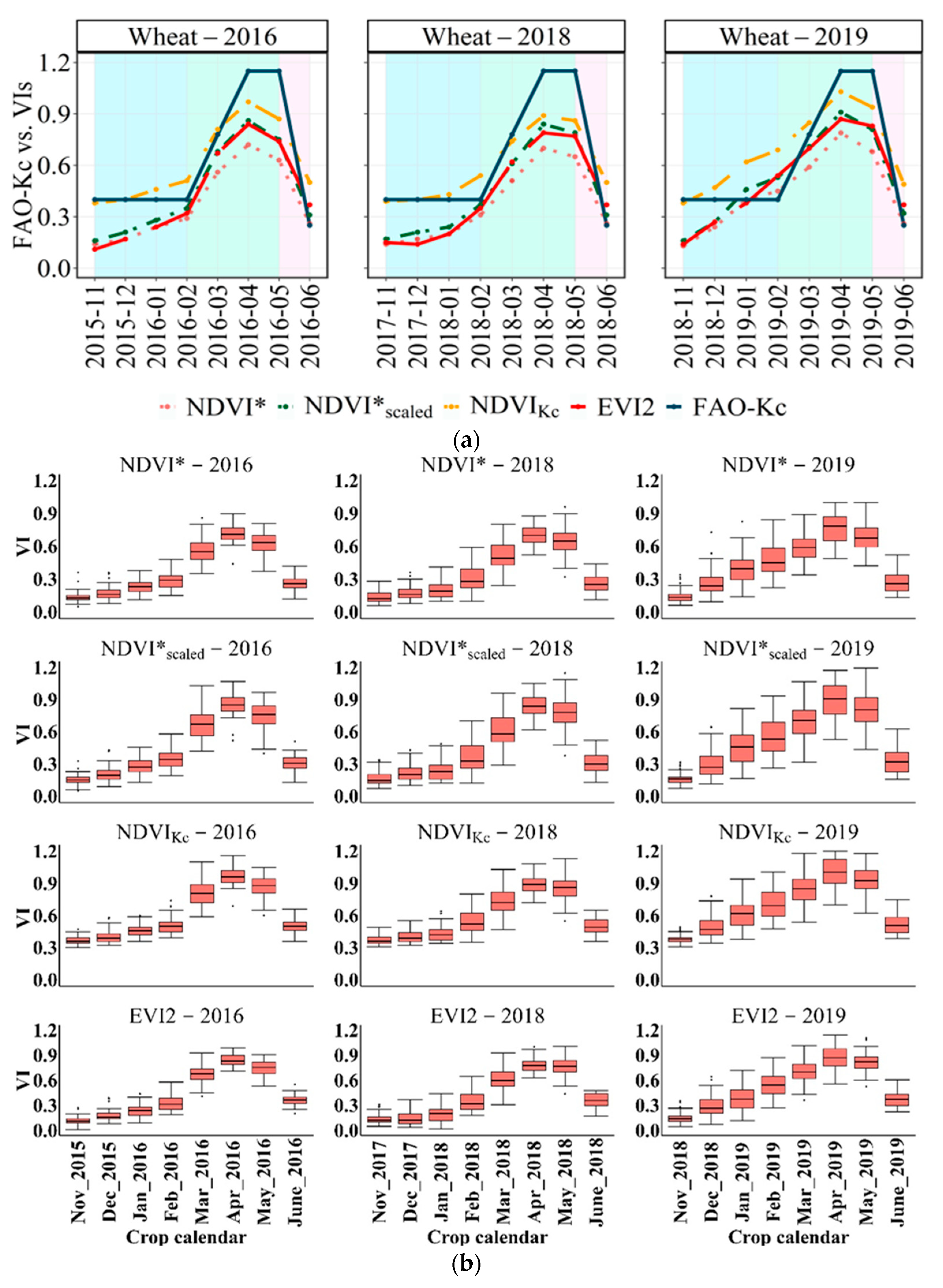
2.4. Evaluation of ET-VIs and VIs

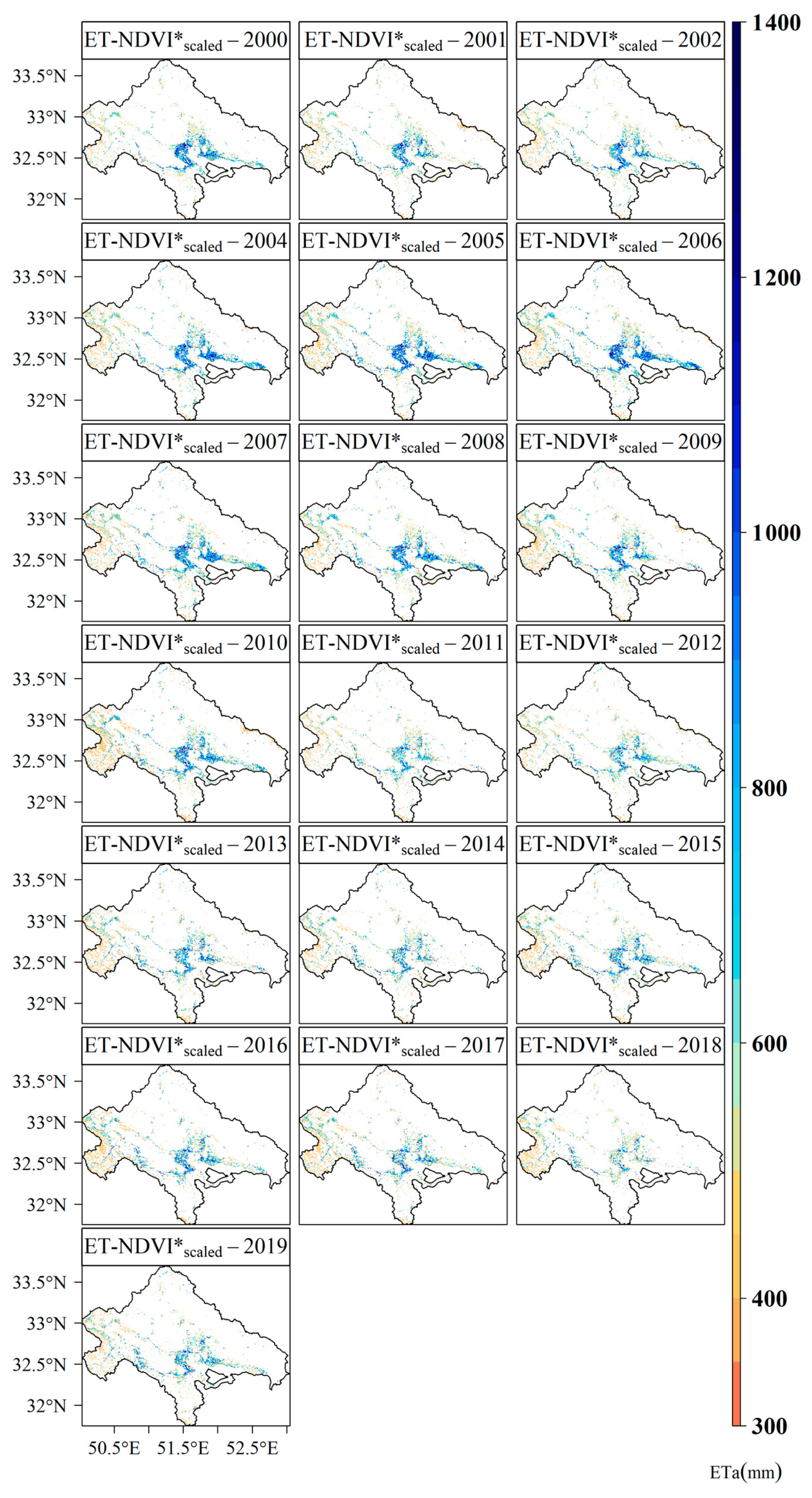
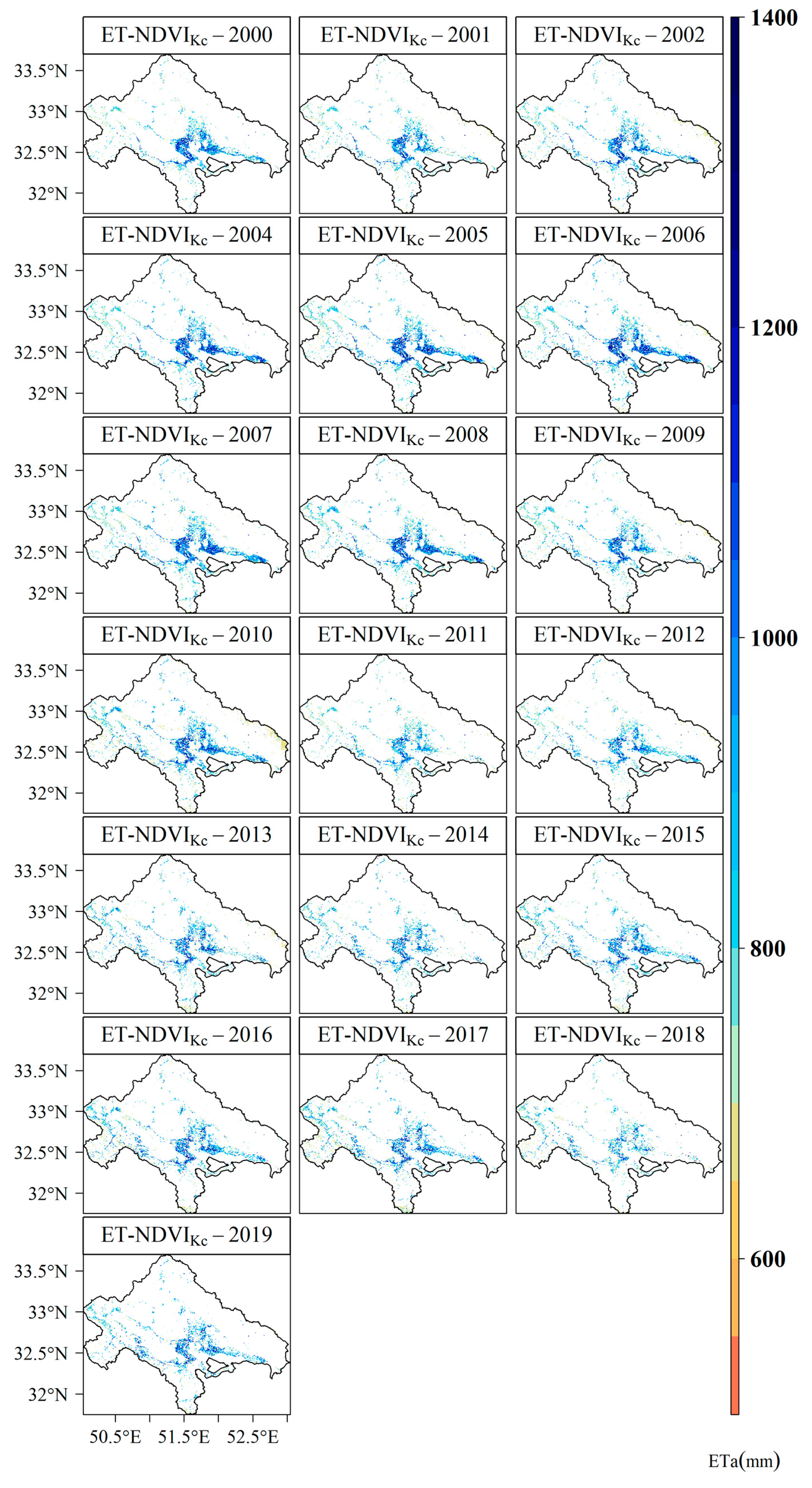
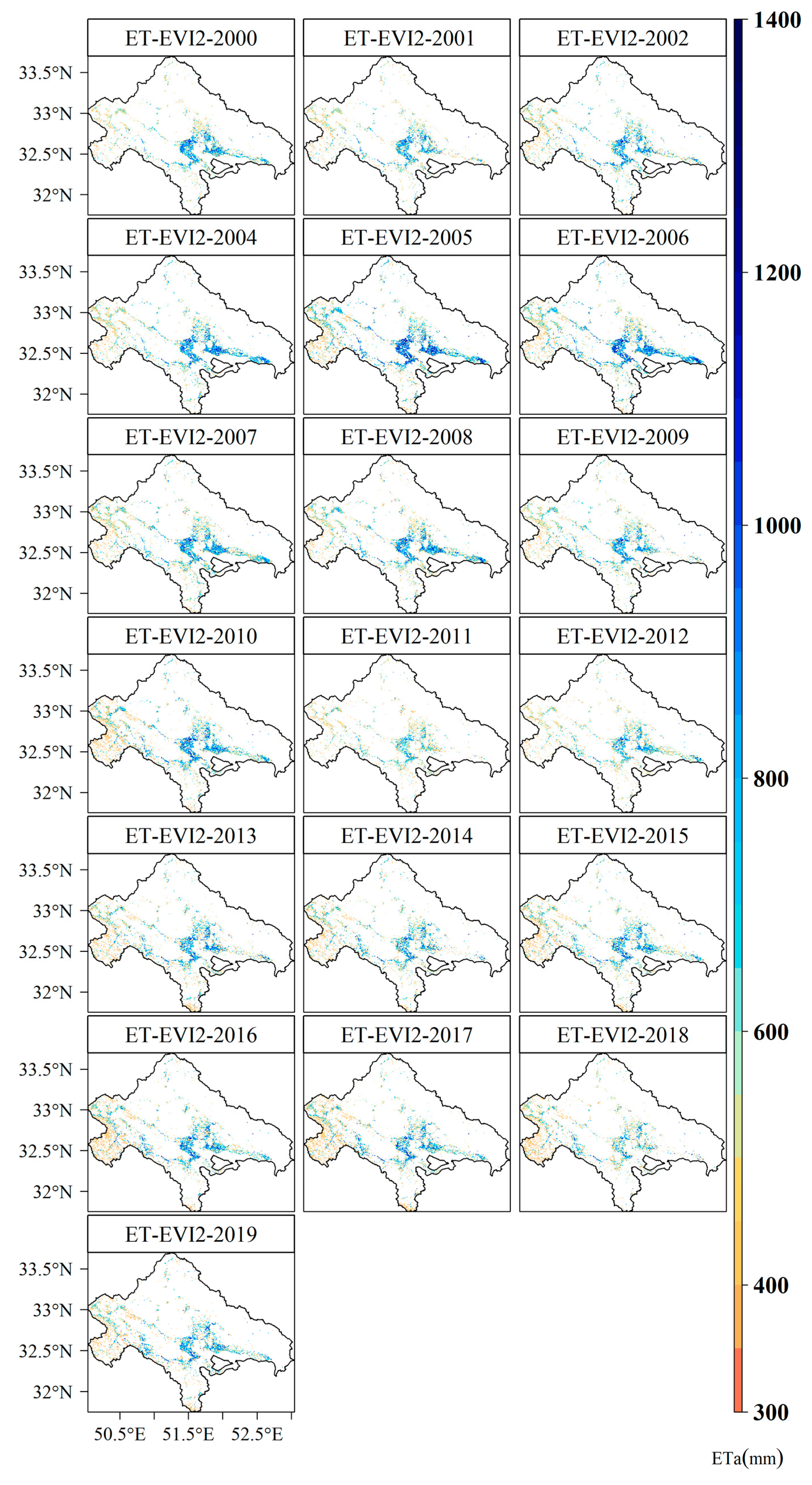
ET-NDVIs were compared with ET-EVI2 and long-term average ETc values; details of ETc calculations were reported by [40]. ET-NDVIs’ performance was evaluated and compared with that of ET-EVI2 using annual average values, annual ET-VIs time series, ETa anomaly (as the deviation from the average ET-VI), and quartile analysis. The Mann–Kendall (MK) test, a non-parametric test, was applied to detect the existence of monotonic trends in the time series of ETa [51]. Since the MK test cannot provide the slope of the trend (magnitude), the Sen method, a nonparametric estimator (S), was used to determine the magnitude of the trend. Negative S values show a descending trend and positive values present an ascending trend [52]. Statistical analysis and visualization of the ET-VIs were conducted in R [53] and QGIS [54].

Ground-truthing data (control point) from wheat farms were collected for the growing season (November–June) over several field visits (2015–2016, 2017–2018, and 2018–2019) by the Isfahan Agriculture Organization (IAO) (https://agri-es.ir/Default.aspx?tabid=1925, accessed on 20 June 2021) in the Isfahan county located in the ZRB. These data were used to evaluate VIs and ET-VIs against the FAO-Kc’s curves and reported ET_wheat for the region by [55], respectively. For this purpose, the corresponding pixel values of VIs and ET-VIs at a monthly scale were extracted at each point across three different growing seasons of wheat (2015–2016, 2017–2018, and 2018–2019). ET-VIs and VIs were then compared to ET_wheat and FAO56-Kc during three growing seasons. Long-term average ETc data (2000–2019) of major crops were also used to determine if the estimated ET-VIs represent the reported ones.

3. Results

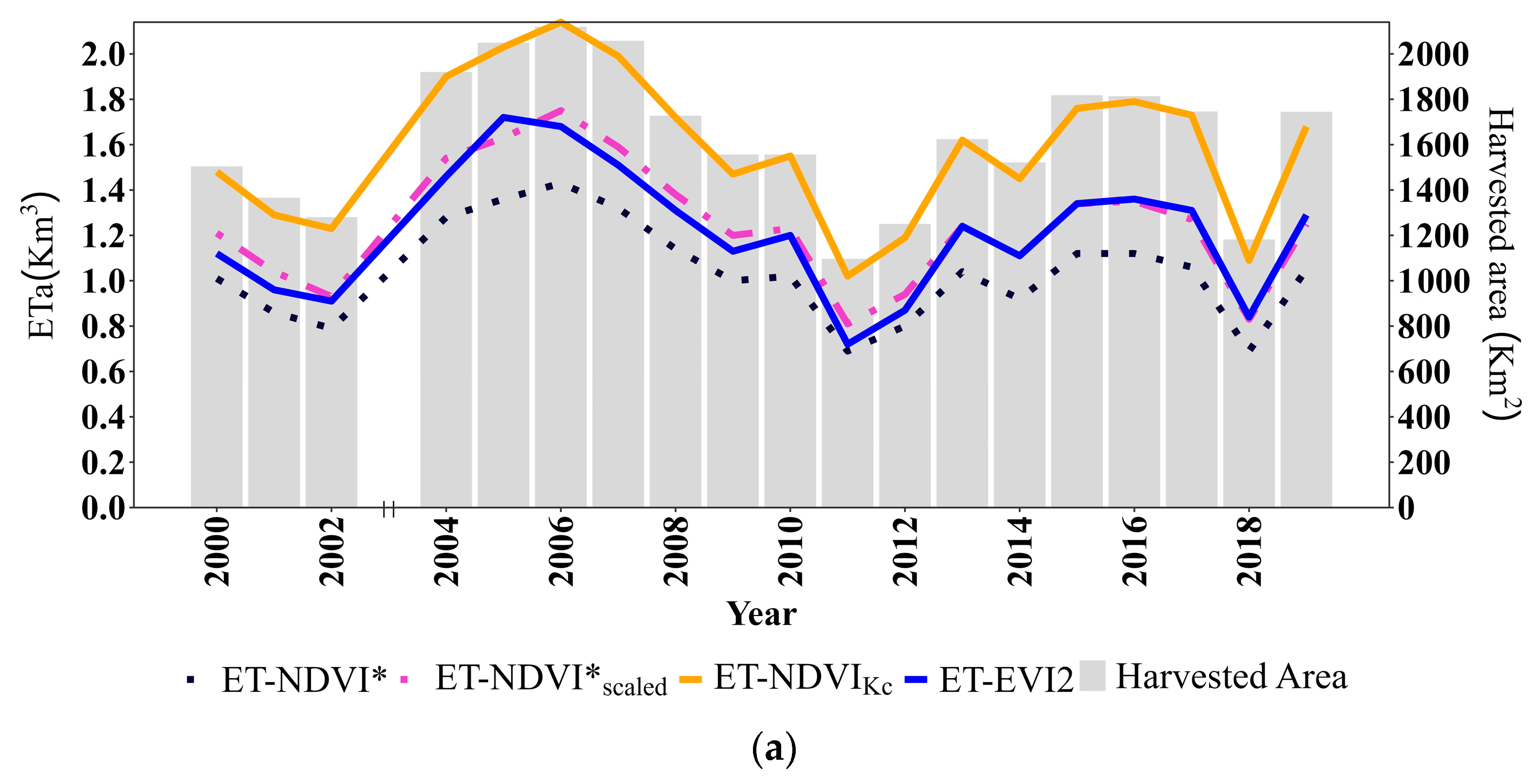
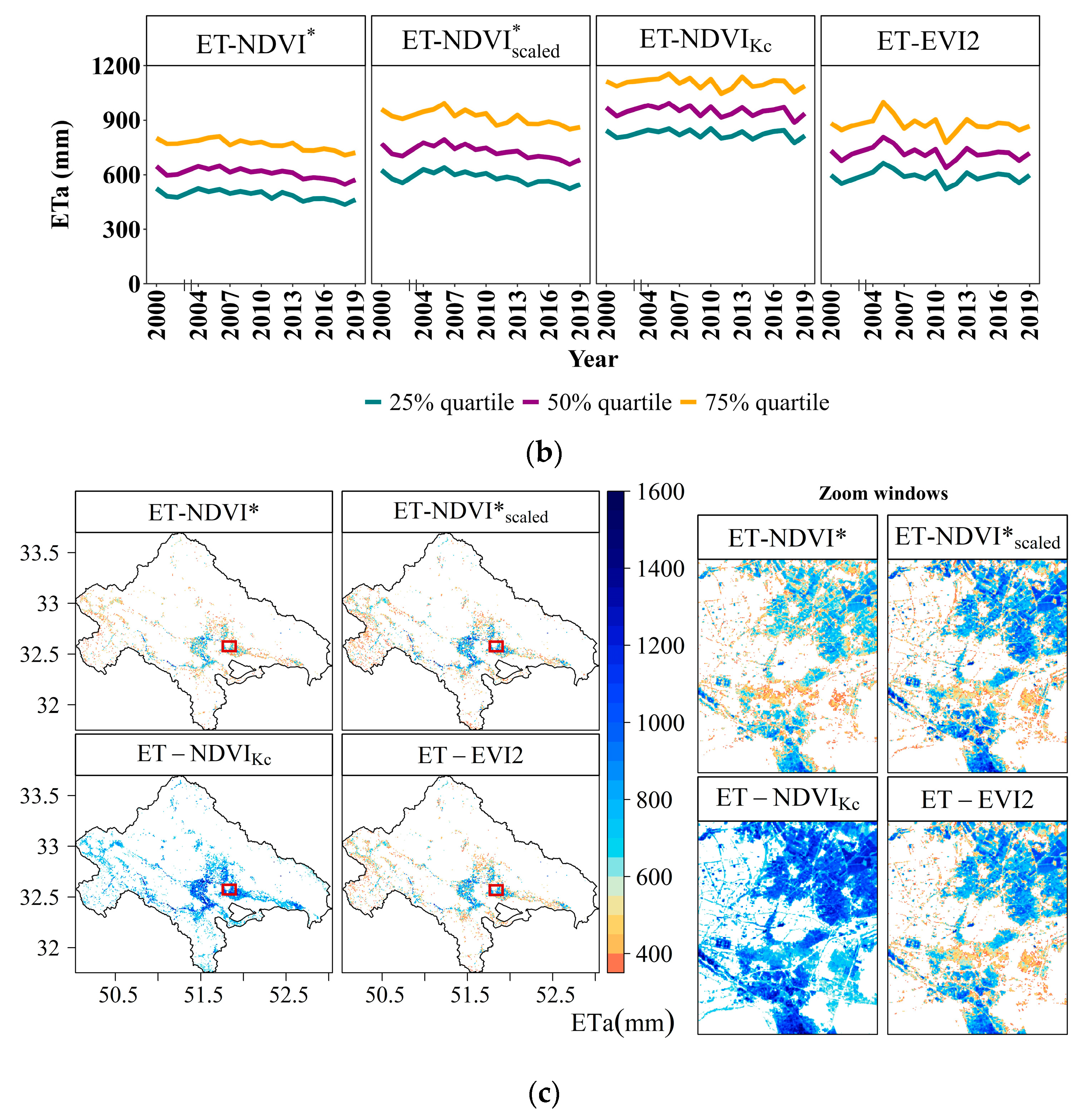
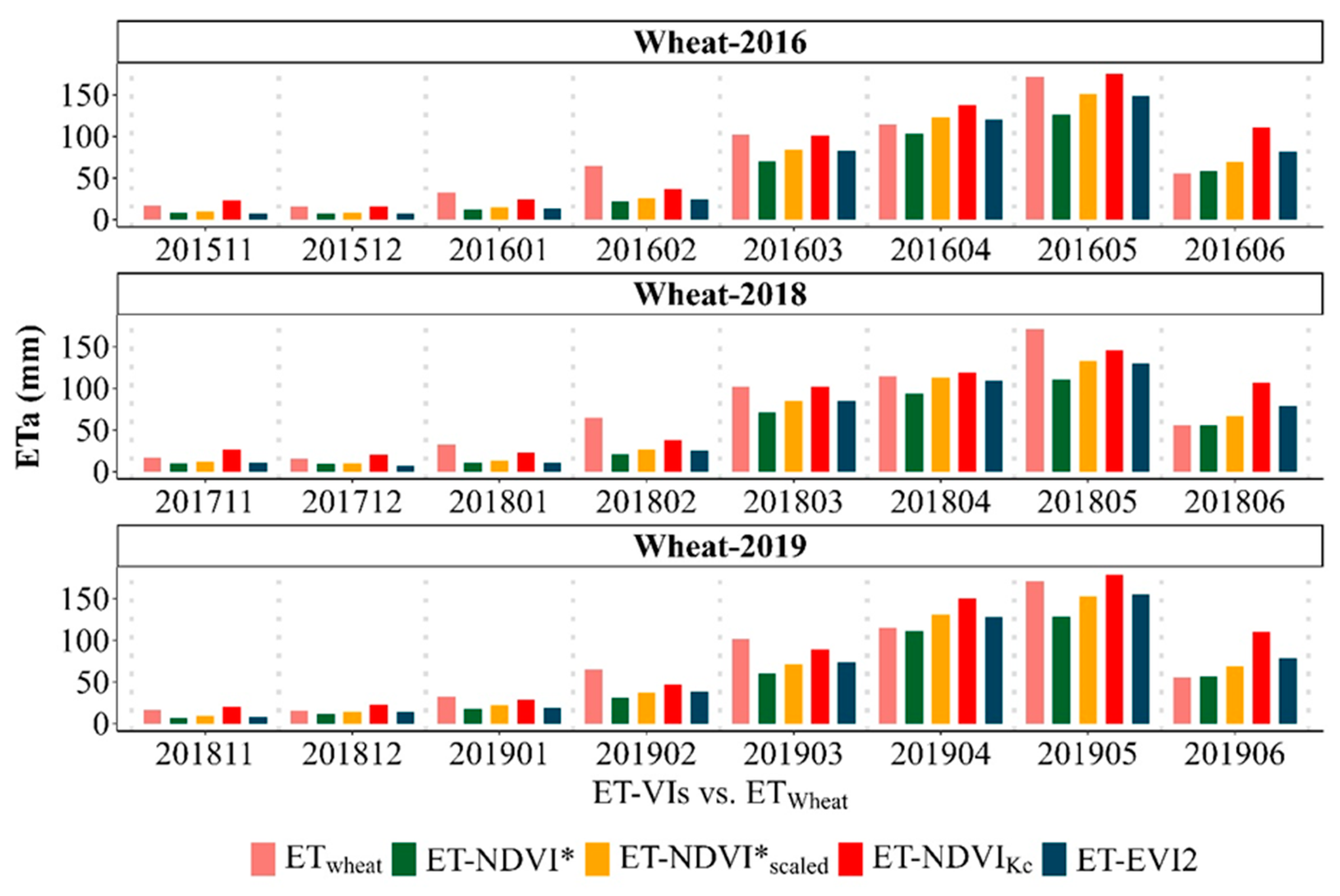
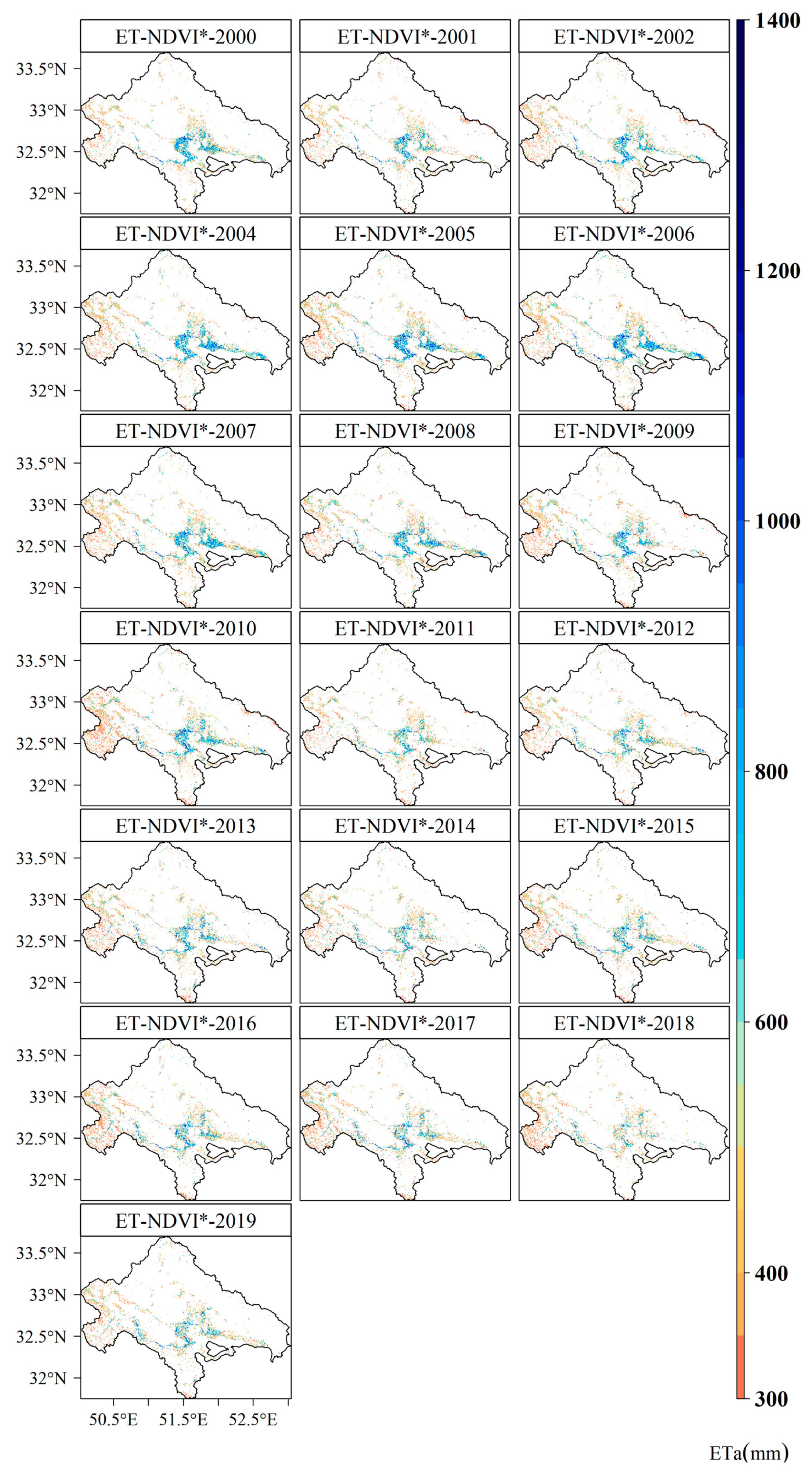
3.1. ETa Products Comparison

Comparing ET-VIs demonstrated that ETa rates are lower in the northwest of the ZRB and higher along the river where croplands are irrigated (Figure 4c; Appendix A: Figure A2, Figure A3, Figure A4 and Figure A5). To show the interannual variability of ETa caused by different cultivated areas, an annual average of the ET-VIs’ volumes (Km³/year) were plotted against the harvested areas’ changes (Figure 4a). Nearly all annual ET-VIs showed that the highest ETa was recorded during 2004–2007 when rainfall was adequate and larger volumes of water were released from the dam to the lower reaches of the ZRB (Figure 4a). ET-VIs, particularly ET-NDVI* and ET-NDVI*_scaled were not significantly sensitive to harvested area changes and dry periods and remained less variable. Figure 4b shows that ET-NDVI*_scaled estimates are closer to ET-EVI2 than those of ET-NDVI* and ET-NDVI_Kc. The lowest and the highest ETa values are those of ET-NDVI* and ET-NDVI_Kc (Figure 4b), respectively. The quartile curves show that the lower and second quartiles of ET-EVI2 and ET-NDVI*_scaled agree with the second and third quartiles of ET-NDVI*. Additionally, the upper quartile of ET-EVI2 and ET-NDVI*_scaled are aligned with the median of ET-NDVI_Kc. The trend analysis of ET-VIs (Appendix A:

Table A1. Trend analysis of ET-VIs. Sen’s slope is in mm/year. The critical Z value at the 5% confidence level is ±1.96, and there is a trend if the MK’s Z value is greater than the Z critical value. Otherwise, the trend is not statistically significant at the confidence level. Additionally, if the p-value is less than the significance level, the null hypothesis is rejected, meaning that there is a trend in the time series [51].

Parameter	ET-NDVI*	ET-NDVI*scaled	ET-NDVIKc	ET-EVI2
Z-Value	−3.54	−3.26	−0.42	−0.32
p-value	0.0004	0.001	0.67	0.75
Sen’s slope	−4	−4.91	−0.58	−0.79
Average	635	760	971	740

) showed a non-significant downward trend for both ET-NDVI_Kc and ET-EVI2, with a decrease of 0.58 and 0.79 mm/year, respectively, while ET-NDVI* and ET-NDVI*_scaled had a significant downward trend (−4 and −4.91 mm/year, respectively). ET-NDVI*_scaled has the highest downward trend based on S with −4.91 mm/year.

3.2. ET-VIs versus Ground-Based Data

To evaluate the ET-VIs’ estimates, long-term average annual ETa estimates were compared with that of reported ETc values (Figure 5a). The results show that all ET-VIs except ET-NDVI* exceeded ETc values. This is because NDVI* has not been scaled to Kc values, therefore ET-NDVI* estimates are lower than other ET-VIs. Among ET-VIs, ET-NDVI* showed the closest values to ETc. ET-NDVI_Kc had the maximum difference compared to ETc, being 328 mm. ET-NDVI* had the lowest deviation from the reported ETc (8 mm) followed by ET-EVI2 and ET-NDVI*_scaled (97 and 117 mm), respectively (Figure 5a). It should be noted that ETc values were calculated within crops’ growing season, while ET-VIs estimates were reported at an annual scale; that is, soil evaporation out of the growing season has not been excluded from the ET-VIs estimate (Figure 5a). Therefore, annual ET-VIs are always larger than the reported ETc. Among scaled VIs, ET-EVI2 followed by ET-NDVI*_scaled showed the lowest difference compared to ETc. We also compared the monthly ETa estimated using RS for three growing seasons with the ETc of wheat reported by [55]. Similarly, ET-EVI2 followed by the scaled ET-NDVI* showed the lowest difference compared to ET_wheat (Figure 5b). The differences increased in 2018 because of a drought event and a significant decrease in wheat cultivation (an almost 80% decline) (Figure 5c).

In the dry year of 2018, ET-VIs are lower than the reported ET_wheat. In 2016, the differences in ET-VIs are close to their corresponding values in 2019. Figure 5a,b show that it is important to consider the growing season in the ETa derivation to avoid ETa overestimation.

A comparison between monthly ET-VIs during three growing seasons and the reported monthly ET_wheat (Figure 6) shows that all ET-VIs’ estimates exceed ET_wheat during the end-stage (in June) in all growing seasons, that is, ET-VIs tend to estimate ETa higher at the end-stage even during the dry year in 2018. Additionally, in April 2016 and 2019 all ET-VIs except ET-NDVI* had a slightly higher ETa. In the early stage (November to January) when evaporation is more dominant than transpiration, almost all ET-VIs estimates were lower than ETc. ET-VIs reached their maximum in May for all growing seasons. From November to February, ET-NDVI*, ET-NDVI*_scaled, and ET-EVI2 have relatively close estimates. A comparison of the monthly average of VIs’ curves as a proxy of Kc values versus FAO-Kc of wheat during three growing seasons (Figure 7a) shows that the VIs’ lowest and highest estimates were from NDVI* and NDVI_Kc, respectively. This is because NDVI* values range between 0 and 1 while other VIs were scaled to reach a maximum of 1.2. FAO-Kc’s values of wheat maximize at 1.15 under no-stress conditions, while in ZRB, due to water scarcity, crops may suffer from water stress even when irrigated and having hardly reached their maximum Kc values. In 2018, VIs’ curves showed a decrease in value at all stages. NDVI_Kc for wheat showed that the minimum Kc value is about 0.4 while the maximum Kc value is 1 (Figure 7a,b). However, other VIs’ minimum values were lower than 0.2 and their maximum values hardly reached 1.

The initial stage in the VI- and FAO-based curves, except for NDVI_Kc, had considerable differences for wheat. All VIs’ estimates exceeded FAO-Kc during the end-stage (in June) in all growing seasons leading to a higher ETa at the end-stage. At the early stage (November to January) and mid-stage (February to May), all VIs’ estimates were lower than FAO-Kc, which reached the highest rate in April during all growing seasons.

4. Discussion

Annual croplands’ ETa was spatially mapped over the ZRB (2000–2019) using GEE platform. We evaluated three NDVI-based ETa (ET-NDVI*, ET-NDVI*_scaled, and ET-NDVI_Kc) and compared them with those of a previously derived ET-EVI2 for the study site [40] and reported ETc values for the ZRB. The VIs, as surrogates for Kc values, were also compared with FAO-Kc. In our study, the comparison of ET-VIs with the long-term averaged ETc revealed that all ET-VIs except ET-NDVI* have higher values of ETa at an annual scale which gives a better picture of the annual water consumption of croplands. The ETa at an annual scale includes ETa values not only within the growing season but also out of the growing season and leads to a higher ETa rate. For the sake of comparison with the field data (reported ETc), we extracted monthly ETa values of our ET-VI products during the growing season and compared them with ET_wheat (2016, 2018, and 2019) to evaluate the performance of ET-VIs. All ET-VIs except ET-NDVI_Kc showed lower values than ET_wheat.

Under well-watered and unstressed conditions, Kc maximizes at 1.2 [41] while NDVI maximizes at 1. Therefore, ET-NDVI* will always have lower ETa estimates. Annual changes in ET-VIs agreed well with each other, however, ET-NDVI* and ET-NDVI*_scaled showed a slightly decreasing trend which can be due to the parameterization and calculation methods. The NDVI*’s results are sensitive when images do not correspond to the maximum vegetation cover [28]. Moreover, this method is suitable under stable conditions and cannot provide reliable estimates in extreme events such as floods and disease outbreaks during parts of the growing season [25]. These major drawbacks make NDVI* and ET-NDVI* more difficult to apply under real-world conditions in the estimation of croplands’ ETa in dry regions. This may not be the case for other land covers such as riparian vegetation [34,38].

Intra-annual cropland changes could capture the drought and water shortage (Figure 8). The climatic conditions in the observation period are characterized by a sequence of normal to wet years (2004–2007) and droughts in the periods 2001–2002, 2011–2012, and 2018 [56], with harvested areas being considerably lower in dry years. Reducing the cultivated areas and keeping lands fallow is a well-known response of farmers to drought in arid and semi-arid regions, particularly in irrigated regions when water resources cannot meet demand. A decrease in the availability of water can also cause soil moisture to decrease and vegetation stress to increase, even in irrigated areas. Our annual ET-VIs’ anomalies (Figure 8) illustrated that all ETa products had similar inter-annual variations with a capability to capture the drought and changes in agricultural areas.

Analysis of the variability of ET-VIs’ anomalies and cropped areas (Figure 8) showed that water stress and drought events affected cultivated areas considerably more than ET-VIs. ETa remained less variable in dry years while cropped areas showed stronger responses with declines of up to 69%. The croplands in the ZRB are inevitably reliant on irrigation. In this region, drought has forced farmers to use their limited available water in a smaller area to safeguard reliable crop production. Marston et el. (2017) reported in a study in the Central Valley of California a 12% reduction in harvested areas through a 3-year successive, exceptional drought leading to the reallocation of limited water supplies from low-value to higher-value crops during the drought [57]. Knowing that drought events affect not only the cropland areas but also yields, particularly in arid and semi-arid regions [58,59], water scarcity has a direct impact on food production (quantity and diversity) and consequently food security.

As opposed to NDVI, EVI2 is less susceptible to saturation and less sensitive to the difference in soil color; this is why EVI2 performs better than NDVI in capturing vegetation conditions and structure changes [60]. Another major advantage of EVI2 is its direct application compared to NDVI* which requires an empirical determination of bare soil inside each scene during the study period. Previous studies support this finding about EVI2 as a better parametrization for ETa estimation in arid and semi-arid regions. Nouri et al. (2020) studied the applicability of three VIs (EVI, EVI2, and NDVI*) in ETa calculation over green spaces in Adelaide, Australia, using three different sensors with different spatial resolutions. Different satellite-based ET-VIs were analyzed and compared with the in-situ data. Their results showed that ET-EVI2 performed well across the three sensors and had the highest correlation with in-situ measurements. Abbasi et al. (2021) analyzed ET-EVI and ET-EVI2 using Landsat imagery over dynamic harvested areas in ZRB. Compared to ETc values, ET-EVI (EVI2) performed well across croplands and are all suitable to monitor ETa in the ZRB. Overall, aligning with the results of our previous study [40], our findings showed that the ET-VIs’ approach and the dynamic cropped areas can be used not only for water and agricultural management, but also for developing and implementing sustainable long-term strategies moving toward a secure water and food future.

Although VI-based methods are simpler and more straightforward [11], they have some sources of error and biases. While the NIR- and the R-reflectance of the visible band—to calculate the VIs—usually have a higher resolution than thermal bands, these bands cannot capture evaporation losses from the soil after irrigation and rainfall [12,23,24]. This introduces some disadvantages when discussing drought and water stress. Although water shortage does not considerably and immediately impact structural properties of the plant [61], NDVI saturates over dense vegetation and is not a reliable indicator for short-term changes in plant water stress. EVI addresses the NDVI saturation, particularly over dense vegetation cover [62] and any remaining residual atmosphere, and it is less sensitive to background noise and atmosphere variability. EVI requires the presence of a blue band, which has a low signal-to-noise and becomes unstable at times; therefore, EVI2 was proposed as an alternative to EVI that does not require the blue band and is less sensitive to noise, making it a much more stable index [60,63]. Thus, VI-based methods are more suitable for long-term ETa estimates, from a monthly to an annual cycle for natural vegetation, unless images with a high temporal resolution are available.

Nevertheless, as with all similar studies, the design of the current study was subjected to some limitations resulting from: (1) lack of sufficient validation data, (2) excluding images in 2003 due to a lack of sufficient images (Appendix A, Figure A1), and (3) using a gridded ETo in this study, as limited access to field observations of ETo might have affected ETa estimates. As of yet, not many studies were conducted in which a sufficient number of stations were installed over a large area to capture the spatial variability of ETo.

5. Conclusions

Our work revealed that ET-EVI2 and ET-NDVI*_scaled agreed well and more closely reproduced reported ETc values. ET-EVI2 and ET-NDVI_Kc are the easiest to apply in other regions, while ET-NDVI* and ET-NDVI*_scaled are scene-dependent by design and therefore require more parameterization and localization. Consequently, we recommend using ET-EVI2 when applying vegetation index-based ETa estimation in semi-arid croplands. Our findings showed that ETa remained less variable in comparison to the cropland areas. In this region, droughts forced farmers to cultivate a smaller area to cope with water shortages; this highlights the fact that less crop water consumption is not necessarily the effect of water-saving strategies, but more so the result of the adjusted crop area. Further investigation is required to precisely understand the reliability of ET-VIs’ estimates across croplands in drylands and examine their crop-specific performance, especially for high-water-consumptive crops such as Alfalfa. In a follow-up study, we plan to assess the translation of our method (ET-EVI2) to other basins in different arid and semi-arid regions and compare it with energy balance methods.

References

1. Misra, A.K. Climate change and challenges of water and food security. Int. J. Sustain. Built Environ. 2014, 3, 153–165. [Google Scholar] [CrossRef]
2. Łabędzki, L.Ł.; Bąk, B. Impact of meteorological drought on crop water deficit and crop yield reduction in Polish agriculture. J. Water Land Dev. 2017, 34, 181–190. [Google Scholar] [CrossRef]
3. Biggs, T.W.; Marshall, M.; Messina, A. Mapping daily and seasonal evapotranspiration from irrigated crops using global climate grids and satellite imagery: Automation and methods comparison. Water Resour. Res. 2016, 52, 7311–7326. [Google Scholar] [CrossRef]
4. Tadesse, T.; Senay, G.B.; Berhan, G.; Regassa, T.; Beyene, S. Evaluating a satellite-based seasonal evapotranspiration product and identifying its relationship with other satellite-derived products and crop yield: A case study for Ethiopia. Int. J. Appl. Earth Obs. Geoinf. 2015, 40, 39–54. [Google Scholar] [CrossRef]
5. Meza, I.; Siebert, S.; Döll, P.; Kusche, J.; Herbert, C.; Eyshi Rezaei, E.; Nouri, H.; Gerdener, H.; Popat, E.; Frischen, J.; et al. Global-scale drought risk assessment for agricultural systems. Nat. Hazards Earth Syst. Sci. 2020, 20, 695–712. [Google Scholar] [CrossRef]
6. Blatchford, M.; Mannaerts, C.M.; Zeng, Y.; Nouri, H.; Karimi, P. Influence of Spatial Resolution on Remote Sensing-Based Irrigation Performance Assessment Using WaPOR Data. Remote Sens. 2020, 12, 2949. [Google Scholar] [CrossRef]
7. Amani, M.; Ghorbanian, A.; Ahmadi, S.A.; Kakooei, M.; Moghimi, A.; Mirmazloumi, S.M.; Moghaddam, S.H.A.; Mahdavi, S.; Ghahremanloo, M.; Parsian, S.; et al. Google Earth Engine Cloud Computing Platform for Remote Sensing Big Data Applications: A Comprehensive Review. IEEE J. Sel. Top. Appl. Earth Obs. Remote Sens. 2020, 13, 5326–5350. [Google Scholar] [CrossRef]
8. Zhang, K.; Kimball, J.S.; Running, S.W. A review of remote sensing based actual evapotranspiration estimation. Wiley Interdiscip. Rev. Water 2016, 3, 834–853. [Google Scholar] [CrossRef]
9. Senay, G.B.; Bohms, S.; Singh, R.K.; Gowda, P.H.; Velpuri, N.M.; Alemu, H.; Verdin, J.P. Operational Evapotranspiration Mapping Using Remote Sensing and Weather Datasets: A New Parameterization for the SSEB Approach. JAWRA J. Am. Water Resour. Assoc. 2013, 49, 577–591. [Google Scholar] [CrossRef]
10. Bastiaanssen, W.G.M.; Cheema, M.J.M.; Immerzeel, W.W.; Miltenburg, I.J.; Pelgrum, H. Surface energy balance and actual evapotranspiration of the transboundary Indus Basin estimated from satellite measurements and the ETLook model. Water Resour. Res. 2012, 48, 1–16. [Google Scholar] [CrossRef] [Green Version]
11. Glenn, E.P.; Nagler, P.L.; Huete, A.R. Vegetation Index Methods for Estimating Evapotranspiration by Remote Sensing. Surv. Geophys. 2010, 31, 531–555. [Google Scholar] [CrossRef]
12. Nagler, P.; Glenn, E.; Nguyen, U.; Scott, R.; Doody, T. Estimating Riparian and Agricultural Actual Evapotranspiration by Reference Evapotranspiration and MODIS Enhanced Vegetation Index. Remote Sens. 2013, 5, 3849–3871. [Google Scholar] [CrossRef]
13. Nouri, H.; Glenn, E.; Beecham, S.; Chavoshi Boroujeni, S.; Sutton, P.; Alaghmand, S.; Noori, B.; Nagler, P. Comparing Three Approaches of Evapotranspiration Estimation in Mixed Urban Vegetation: Field-Based, Remote Sensing-Based and Observational-Based Methods. Remote Sens. 2016, 8, 492. [Google Scholar] [CrossRef]
14. Allen, R.G.; Pereira, L.S.; Raes, D.; Smith, M. Crop Evapotranspiration: Guidelines for Computing Crop Water Requirements; Food and Agriculture Organization of the United States: Rome, Italy, 1988; ISBN 9251042195. [Google Scholar]
15. Sishodia, R.P.; Ray, R.L.; Singh, S.K. Applications of Remote Sensing in Precision Agriculture: A Review. Remote Sens. 2020, 12, 3136. [Google Scholar] [CrossRef]
16. Allen, R. Using the FAO-56 dual crop coefficient method over an irrigated region as part of an evapotranspiration intercomparison study. J. Hydrol. 2000, 229, 27–41. [Google Scholar] [CrossRef]
17. Nouri, H.; Beecham, S.; Kazemi, F.; Hassanli, A.M.; Anderson, S. Remote sensing techniques for predicting evapotranspiration from mixed vegetated surfaces. Hydrol. Earth Syst. Sci. Discuss. 2013, 10, 3897–3925. [Google Scholar] [CrossRef]
18. Akdim, N.; Alfieri, S.; Habib, A.; Choukri, A.; Cheruiyot, E.; Labbassi, K.; Menenti, M. Monitoring of Irrigation Schemes by Remote Sensing: Phenology versus Retrieval of Biophysical Variables. Remote Sens. 2014, 6, 5815–5851. [Google Scholar] [CrossRef]
19. Hunsaker, D.J.; Pinter, P.J.; Barnes, E.M.; Kimball, B.A. Estimating cotton evapotranspiration crop coefficients with a multispectral vegetation index. Irrig Sci 2003, 22, 95–104. [Google Scholar] [CrossRef]
20. Nagler, P.; Morino, K.; Murray, R.S.; Osterberg, J.; Glenn, E. An Empirical Algorithm for Estimating Agricultural and Riparian Evapotranspiration Using MODIS Enhanced Vegetation Index and Ground Measurements of ET. I. Description of Method. Remote Sens. 2009, 1, 1273–1297. [Google Scholar] [CrossRef]
21. Murray, R.S.; Nagler, P.; Morino, K.; Glenn, E. An Empirical Algorithm for Estimating Agricultural and Riparian Evapotranspiration Using MODIS Enhanced Vegetation Index and Ground Measurements of ET. II. Application to the Lower Colorado River, U.S. Remote Sens. 2009, 1, 1125–1138. [Google Scholar] [CrossRef] [Green Version]
22. Glenn, E.P.; Neale, C.M.U.; Hunsaker, D.J.; Nagler, P.L. Vegetation index-based crop coefficients to estimate evapotranspiration by remote sensing in agricultural and natural ecosystems. Hydrol. Process. 2011, 25, 4050–4062. [Google Scholar] [CrossRef]
23. French, A.N.; Hunsaker, D.J.; Sanchez, C.A.; Saber, M.; Gonzalez, J.R.; Anderson, R. Satellite-based NDVI crop coefficients and evapotranspiration with eddy covariance validation for multiple durum wheat fields in the US Southwest. Agric. Water Manag. 2020, 239, 106266. [Google Scholar] [CrossRef]
24. Nagler, P.; Scott, R.; Westenburg, C.; Cleverly, J.; Glenn, E.; Huete, A. Evapotranspiration on western U.S. rivers estimated using the Enhanced Vegetation Index from MODIS and data from eddy covariance and Bowen ratio flux towers. Remote Sens. Environ. 2005, 97, 337–351. [Google Scholar] [CrossRef]
25. Khand, K.; Taghvaeian, S.; Hassan-Esfahani, L. Mapping Annual Riparian Water Use Based on the Single-Satellite-Scene Approach. Remote Sens. 2017, 9, 832. [Google Scholar] [CrossRef]
26. Nagler, P.L.; Barreto-Muñoz, A.; Chavoshi Borujeni, S.; Nouri, H.; Jarchow, C.J.; Didan, K. Riparian Area Changes in Greenness and Water Use on the Lower Colorado River in the USA from 2000 to 2020. Remote Sens. 2021, 13, 1332. [Google Scholar] [CrossRef]
27. Nagler, P.; Sall, I.; Barreto-Muñoz, A.; Gómez-Sapiens, M.; Nouri, H.; Chavoshi Borujeni, S.; Didan, K. Effect of restoration on plant greenness and water use in relation to drought in the riparian corridor of the Colorado River delta. J. Am. Water Resour. Assoc. 2022, 58, 746–784. [Google Scholar] [CrossRef]
28. Jarchow, C.J.; Waugh, W.J.; Nagler, P.L. Calibration of an evapotranspiration algorithm in a semiarid sagebrush steppe using a 3-ha lysimeter and Landsat normalized difference vegetation index data. Ecohydrology 2022, 15. [Google Scholar] [CrossRef]
29. Nouri, H.; Beecham, S.; Anderson, S.; Nagler, P. High Spatial Resolution WorldView-2 Imagery for Mapping NDVI and Its Relationship to Temporal Urban Landscape Evapotranspiration Factors. Remote Sens. 2014, 6, 580–602. [Google Scholar] [CrossRef]
30. Vulova, S.; Meier, F.; Rocha, A.D.; Quanz, J.; Nouri, H.; Kleinschmit, B. Modeling urban evapotranspiration using remote sensing, flux footprints, and artificial intelligence. Sci. Total Environ. 2021, 786, 147293. [Google Scholar] [CrossRef] [PubMed]
31. Bausch, W.C.; Neale, C.M.U. Crop Coefficients Derived from Reflected Canopy Radiation: A Concept. Trans. ASAE 1987, 30, 703–709. [Google Scholar] [CrossRef]
32. Kamble, B.; Kilic, A.; Hubbard, K. Estimating Crop Coefficients Using Remote Sensing-Based Vegetation Index. Remote Sens. 2013, 5, 1588–1602. [Google Scholar] [CrossRef]
33. Duchemin, B.; Hadria, R.; Erraki, S.; Boulet, G.; Maisongrande, P.; Chehbouni, A.; Escadafal, R.; Ezzahar, J.; Hoedjes, J.; Kharrou, M.H.; et al. Monitoring wheat phenology and irrigation in Central Morocco: On the use of relationships between evapotranspiration, crops coefficients, leaf area index and remotely-sensed vegetation indices. Agric. Water Manag. 2006, 79, 1–27. [Google Scholar] [CrossRef]
34. Groeneveld, D.P.; Baugh, W.M. Correcting satellite data to detect vegetation signal for eco-hydrologic analyses. J. Hydrol. 2007, 344, 135–145. [Google Scholar] [CrossRef]
35. Senay, G.B.; Leake, S.; Nagler, P.L.; Artan, G.; Dickinson, J.; Cordova, J.T.; Glenn, E.P. Estimating basin scale evapotranspiration (ET) by water balance and remote sensing methods. Hydrol. Process. 2011, 25, 4037–4049. [Google Scholar] [CrossRef]
36. Jarchow, C.J.; Nagler, P.L.; Glenn, E.P. Greenup and evapotranspiration following the Minute 319 pulse flow to Mexico: An analysis using Landsat 8 Normalized Difference Vegetation Index (NDVI) data. Ecol. Eng. 2017, 106, 776–783. [Google Scholar] [CrossRef]
37. Bresloff, C.J.; Nguyen, U.; Glenn, E.P.; Waugh, J.; Nagler, P.L. Effects of grazing on leaf area index, fractional cover and evapotranspiration by a desert phreatophyte community at a former uranium mill site on the Colorado Plateau. J. Environ. Manag. 2013, 114, 92–104. [Google Scholar] [CrossRef]
38. Jarchow, C.J.; Waugh, W.J.; Didan, K.; Barreto-Muñoz, A.; Herrmann, S.; Nagler, P.L. Vegetation-groundwater dynamics at a former uranium mill site following invasion of a biocontrol agent: A time series analysis of Landsat normalized difference vegetation index data. Hydrol. Process. 2020, 34, 2739–2749. [Google Scholar] [CrossRef]
39. Nouri, H.; Nagler, P.; Chavoshi Borujeni, S.; Barreto Munez, A.; Alaghmand, S.; Noori, B.; Galindo, A.; Didan, K. Effect of spatial resolution of satellite images on estimating the greenness and evapotranspiration of urban green spaces. Hydrol. Process. 2020, 34, 3183–3199. [Google Scholar] [CrossRef]
40. Abbasi, N.; Nouri, H.; Didan, K.; Barreto-Muñoz, A.; Chavoshi Borujeni, S.; Salemi, H.; Opp, C.; Siebert, S.; Nagler, P. Estimating Actual Evapotranspiration over Croplands Using Vegetation Index Methods and Dynamic Harvested Area. Remote Sens. 2021, 13, 5167. [Google Scholar] [CrossRef]
41. D’Urso, G. Current Status and Perspectives for the Estimation of Crop Water Requirements from Earth Observation. Ital. J. Agron. 2010, 5, 107. [Google Scholar] [CrossRef] [Green Version]
42. Allen, R.G.; Pereira, L.S.; Howell, T.A.; Jensen, M.E. Evapotranspiration information reporting: I. Factors governing measurement accuracy. Agric. Water Manag. 2011, 98, 899–920. [Google Scholar] [CrossRef]
43. Belmonte, A.C.; Jochum, A.M.; GarcÍa, A.C.; Rodríguez, A.M.; Fuster, P.L. Irrigation management from space: Towards user-friendly products. Irrig Drain. Syst 2005, 19, 337–353. [Google Scholar] [CrossRef]
44. Mohammadian, M.; Arfania, R.; Sahour, H. Evaluation of SEBS Algorithm for Estimation of Daily Evapotranspiration Using Landsat-8 Dataset in a Semi-Arid Region of Central Iran. Open, J. Geol. 2017, 07, 335–347. [Google Scholar] [CrossRef]
45. Zamani, O.; Grundmann, P.; Libra, J.A.; Nikouei, A. Limiting and timing water supply for agricultural production—The case of the Zayandeh-Rud River Basin, Iran. Agric. Water Manag. 2019, 222, 322–335. [Google Scholar] [CrossRef]
46. Sarvari, H.; Rakhshanifar, M.; Tamošaitienė, J.; Chan, D.W.; Beer, M. A Risk Based Approach to Evaluating the Impacts of Zayanderood Drought on Sustainable Development Indicators of Riverside Urban in Isfahan-Iran. Sustainability 2019, 11, 6797. [Google Scholar] [CrossRef]
47. Gohari, A.; Eslamian, S.; Abedi-Koupaei, J.; Massah Bavani, A.; Wang, D.; Madani, K. Climate change impacts on crop production in Iran’s Zayandeh-Rud River Basin. Sci. Total Environ. 2013, 442, 405–419. [Google Scholar] [CrossRef] [PubMed]
48. Gorelick, N.; Hancher, M.; Dixon, M.; Ilyushchenko, S.; Thau, D.; Moore, R. Google Earth Engine: Planetary-scale geospatial analysis for everyone. Remote Sens. Environ. 2017, 202, 18–27. [Google Scholar] [CrossRef]
49. Roy, D.P.; Kovalskyy, V.; Zhang, H.K.; Vermote, E.F.; Yan, L.; Kumar, S.S.; Egorov, A. Characterization of Landsat-7 to Landsat-8 reflective wavelength and normalized difference vegetation index continuity. Remote Sens. Environ. 2016, 185, 57–70. [Google Scholar] [CrossRef] [PubMed]
50. Nagler, P.L.; Barreto-Muñoz, A.; Chavoshi Borujeni, S.; Jarchow, C.J.; Gómez-Sapiens, M.M.; Nouri, H.; Herrmann, S.M.; Didan, K. Ecohydrological responses to surface flow across borders: Two decades of changes in vegetation greenness and water use in the riparian corridor of the Colorado River delta. Hydrol. Process. 2020, 34, 4851–4883. [Google Scholar] [CrossRef]
51. Hamed, K.H.; Ramachandra Rao, A. A modified Mann-Kendall trend test for autocorrelated data. J. Hydrol. 1998, 204, 182–196. [Google Scholar] [CrossRef]
52. Sen, P.K. Estimates of the regression coefficient based on Kendall’s tau. J. Am. Stat. 1968, 63, 1379–1389. [Google Scholar] [CrossRef]
53. R Core Team. A Language and Environment for Statistical Computing; R Foundation for Statistical Computing: Vienna, Austria, 2021. [Google Scholar]
54. QGIS.org. QGIS Geographic Information System; QGIS Association, 2022. Available online: http://www.qgis.org (accessed on 2 February 2022).
55. Salemi, H.; Toomanian, N.; Jalali, A.; Nikouei, A.; Khodagholi, M.; Rezaei, M. Determination of Net Water Requirement of Crops and Gardens in Order to Optimize the Management of Water Demand in Agricultural Sector; Springer: Cham, Switzerand, 2020; pp. 331–360. [Google Scholar] [CrossRef]
56. Karamouz, M.; Rasouli, K.; Nazif, S. Development of a Hybrid Index for Drought Prediction: Case Study. J. Hydrol. Eng. 2009, 14, 617–627. [Google Scholar] [CrossRef]
57. Marston, L.; Konar, M. Drought impacts to water footprints and virtual water transfers of the C entral V alley of C alifornia. Water Resour. Res. 2017, 53, 5756–5773. [Google Scholar] [CrossRef]
58. Rezaei, E.E.; Ghazaryan, G.; Moradi, R.; Dubovyk, O.; Siebert, S. Crop harvested area, not yield, drives variability in crop production in Iran. Environ. Res. Lett. 2021, 16, 64058. [Google Scholar] [CrossRef]
59. Lesk, C.; Rowhani, P.; Ramankutty, N. Influence of extreme weather disasters on global crop production. Nature 2016, 529, 84–87. [Google Scholar] [CrossRef] [PubMed]
60. Jiang, Z.; Huete, A.R.; Kim, Y.; Didan, K. 2-band enhanced vegetation index without a blue band and its application to AVHRR data. In Remote Sensing and Modeling of Ecosystems for Sustainability IV; Optical Engineering + Applications; Gao, W., Ustin, S.L., Eds.; SPIE: San Diego, CA, USA, 2007; p. 667905. [Google Scholar]
61. Moran, M.S.; Clarke, T.R.; Inoue, Y.; Vidal, A. Estimating crop water deficit using the relation between surface-air temperature and spectral vegetation index. Remote Sens. Environ. 1994, 49, 246–263. [Google Scholar] [CrossRef]
62. Huete, A.; DIDAN, K.; MIURA, T.; Rodriguez, E.; Gao, X.; Ferreira, L. Overview of the radiometric and biophysical performance of the MODIS vegetation indices. Remote Sens. Environ. 2002, 83, 195–213. [Google Scholar] [CrossRef]
63. Jiang, Z.; Huete, A.; DIDAN, K.; MIURA, T. Development of a two-band enhanced vegetation index without a blue band. Remote Sens. Environ. 2008, 112, 3833–3845. [Google Scholar] [CrossRef]
Figure 1. (a) The Zayandehrud River basin (ZRB), (b) Annual average precipitation upstream and downstream of the ZRB, (c) Climograph of the ZRB: Long-term monthly average precipitation and temperature.
Remotesensing 15 01017 g001
Figure 2. Workflow: green color presents the products developed in this study, blue color shows external data used in this study to assess performance of ET-NDVIs.
Remotesensing 15 01017 g002
Figure 3. An example of the calculation of x-intercept for one scene.
Remotesensing 15 01017 g003
Figure 4. Comparison of ET-VIs, (a) Annual ET-VIs (volume in km3) vs. cultivated area over time, (b) Annual ET-VIs’ first, median, and third quartile, and (c) Long-term ET-VIs’ map with zoom windows of the red boxes inside the maps have been shown on the left to better illustrate the differences between ET-VIs.
Remotesensing 15 01017 g004aRemotesensing 15 01017 g004b
Figure 5. Comparing ET-VIs with ETc and ETwheat: (a) Comparing long-term average ET-VIs with reported ETc; light green: growing season scale; dark green: annual scale. (b) Comparing ET-VIs with ETwheat within three different growing seasons; numbers on bars show the difference between ET-VIs and ETwheat, and (c) Cultivated area of wheat from 2015 to 2019.
Remotesensing 15 01017 g005
Figure 6. Comparison of monthly ET-VIs in three growing seasons with reported long-term monthly ETwheat.
Remotesensing 15 01017 g006
Figure 7. (a) Comparison of FAO-Kc with VI, background colors show different crop growth stages, i.e., blue: initial stage, green: middle stage, pink: end-stage; (b) Boxplots of estimated VIs of wheat during growing seasons.
Remotesensing 15 01017 g007
Figure 8. Annual harvested areas change (green bar chart) vs. annual ET-VIs’ anomaly (boxplots) over harvested areas.
Remotesensing 15 01017 g008
Disclaimer/Publisher’s Note: The statements, opinions and data contained in all publications are solely those of the individual author(s) and contributor(s) and not of MDPI and/or the editor(s). MDPI and/or the editor(s) disclaim responsibility for any injury to people or property resulting from any ideas, methods, instructions or products referred to in the content.