Article

Refining the Resolution of DUACS Along-Track Level-3 Sea Level Altimetry Products

1
CLS, 11 rue Hermès, Parc Technologique du Canal, 31520 Ramonville St. Agne, France
2
IMEDEA, C/Miquel Marquès, 21-07190 Esporles, Illes Balears, Spain
3
CNES, 18 Avenue Edouard Belin, CEDEX 9, 31401 Toulouse, France
*
Author to whom correspondence should be addressed.
Remote Sens. 2023, 15(3), 793; https://doi.org/10.3390/rs15030793
Submission received: 20 December 2022 / Revised: 20 January 2023 / Accepted: 20 January 2023 / Published: 30 January 2023

Abstract

:
This paper describes the demonstration of a regional high-resolution level-3 (L3) altimeter data unification and altimeter combination system (DUACS) developed with support from the French space agency (CNES). Deduced from full-rate (20 Hz to 40 Hz) level-2 (L2) altimeter measurements, this product provides sea level anomalies (SLA) and other essential physical variables at a spatial resolution of one sample every ~1 km over the North Atlantic Ocean. This allows us to resolve wavelengths from ~35 km to ~55 km depending on the altimeter considered. This was made possible by recent advances in radar altimeter processing for both synthetic aperture radar (SAR) and low-resolution-mode (LRM) measurements, as well as improvements made to different stages of the DUACS processing chain. Firstly, the new adaptive and low-resolution with range migration correction (LR-RMC) processing techniques were considered for Jason and Sentinel-3 (S3A), respectively. They significantly reduce errors at short wavelengths, and the adaptive processing also reduces possible land contamination near the coast. Next, up-to-date geophysical and environmental corrections were selected for this production. This includes specific corrections intended to reduce the measurement noise on LRM measurements and thus enhance the observability at short wavelengths. Compared with the 1 Hz product, the observable wavelengths reached with the demonstration high-resolution product are reduced by up to one third, or up to half in the northeast Atlantic region. The residual noises were optimally filtered from full-rate measurements, taking into consideration the different observing capabilities of the altimeters processed. A specific data recovery strategy was applied, significantly optimizing the data availability, both in the coastal and open ocean areas. This demonstration L3 product is thus better resolved than the conventional 1 Hz product, especially near the coast, where it is defined up to ~5 km against ~10 km for the 1 Hz version. Multi-mission cross-calibration processing was also optimized with an improved long-wavelength error (LWE) correction, leading to a better consistency between tracks, with a 9–15% reduction in SLA variance at cross-overs. The new L3 product improves the overall consistency with tide gauge measurements, with a reduction in SLA differences variance by 5 and 17% compared with the 1 Hz product from the S3A and Jason-3 (J3) measurements, respectively. Primarily intended for regional applications, this product can significantly contribute to improving high-resolution numerical model output via data assimilation. It also opens new perspectives for a better understanding of regional sea-surface dynamics, with an improved representation of the coastal currents and a refined spectral content revealing the unbalanced signal.
Keywords:
altimetry; mesoscale

1. Introduction

As part of the CNES/SALP (Centre National d’Etudes Spatiales/Service d’Altimetrie et Localisation Precise) project and the Copernicus Marine Environment and Monitoring Service (CMEMS), the DUACS system produces high-quality multi-mission altimetry sea level products for ocean applications, climate monitoring, geophysical and biological studies. These products consist of directly usable and easy to manipulate level-3 (L3; along-track cross-calibrated sea-surface height) and level-4 (L4; multiple sensors merged as maps or time series) products. They are widely used for different applications, including assimilation in numerical models. In the past few years, DUACS products have been regularly updated in order to deliver products of the highest quality, based on the state-of-the-art processing algorithms and improvements, as well as newly available measurements [1,2,3,4,5]. Despite these advances, the effective resolution of the DUACS altimeter products remains low with regard to the new requirements made by different applications [6,7,8,9].
Indeed, advances in the small (from ~200 to 100 km) to sub-mesoscale (<~100 km) sea-surface dynamical processes have given new insight into the importance of this signal in the ocean’s dynamics [10,11,12,13,14]. At the same time, the monitoring of sea level changes in coastal areas is an important societal issue. Because altimeter measurements allow for synoptic monitoring of the signal over the global ocean, including coasts, they are fundamental for both sub-mesoscale and coastal applications. The processing of altimeter data now faces a new challenge in accurately processing the signal at yet finer spatial scales than hitherto considered. This issue will be even more critical for future altimeter missions, such as the swath Surface Water and Ocean Topography (SWOT) mission. In the same way, altimeter measurement processing needs to evolve in order to better resolve the signal in coastal areas. Meanwhile, users and, more particularly, modelers, are also upgrading their models to resolve small-scale processes at a regional scale. To this end, they will need to prepare their systems for the assimilation and propagation of the finer-scale structures observed.
The land contamination affecting both altimeter radars and radiometer measurements, which is associated with the degradation of the different corrections that need to be applied to altimeter measurements, as well as the predominance of residual errors at short wavelengths, have significantly reduced the quality of altimeter products for such applications for many years (e.g., [15,16]).
Nevertheless, over the last decade, significant improvements have been made in the estimation of different geophysical corrections. Advances in atmospheric and barotropic ocean models have allowed for more accurate corrections of the ocean’s response to wind and pressure forcing (e.g., [17]); progress in modeling and assimilation techniques have contributed to more accurate barotropic ocean tide corrections (e.g., [18]); new model corrections have also emerged and have allowed us to correct part of the coherent internal gravity wave signal (e.g., [19]); tropospheric corrections, enhanced in coastal areas, are also available (e.g., [20,21]); and progress has also been made in the determination of the mean sea surface (MSS) field, which is still a fundamental part of altimeter data processing [22,23]. Major advances made in altimeter technologies and processing have also significantly contributed to reducing altimeter measurement errors. First, the Ka band used for SARAL/AltiKa significantly reduced the measurement noise on conventional LRM altimetry [24]. For a few years already, the SAR technology available on the Cryosat-2 (C2) and Sentinel-3 missions has also contributed to an unprecedented reduction in the observational errors at short wavelengths (e.g., [25,26]). New processing techniques have been developed to enhance SAR capabilities and reduce the residual red noise induced by long ocean waves [27,28,29]. In the same way, new waveform retracking techniques have allowed us to reduce residual noise levels in LRM measurements and even better adapt the model to the waveform shape characteristics of different sea-surface states and land/ice contamination [30,31,32,33]. Recent progress made in sea-state bias correction has also contributed to reducing the measurement noise [34,35]. Additionally, corrections have been developed to specifically reduce signal noise at short wavelengths [35,36,37,38].
In light of these developments and the associated reduction in the errors at short wavelengths, full-rate altimeter measurements can now be used to access the small-mesoscale signal and better sample difficult areas, such as coastal zones or leads. Different regional altimeter products have been developed over the last few years with the aim of focusing on the coastal zone (e.g., PISTACH [39]; X-TRACK [40,41]; X-TRACK-ALES [42]; ESA EO4SIBS [43]). Others are dedicated to ice-contaminated areas, focusing on the sea surface over leads [44,45]. In this paper, we focus on the DUACS high-resolution L3 altimeter demonstration’s regional products, which are primarily intended for high-resolution regional model applications and guided by the CMEMS requirements. These products have been developed in a CNES R&D context with the aim of preparing the future generation of L3 altimeter products that may be disseminated operationally in the CMEMS catalogue. In contrast with the current 1 Hz L3 product available in CMEMS, this new L3 product is defined with a 5 Hz sampling rate and derived from a high-resolution (20 Hz) altimeter measurement (Sentinel-3A, Jason-3, OSTM/Jason-2, Cryosat-2, SARAL-DP/AltiKa) specifically processed in order to better resolve finer scales down to ~35 km (the current observable wavelengths for L3 1 Hz are estimated to be 65 km in mid-latitude areas [1]).
The paper is organized as follows: In Section 2, the processing and different corrections used are described. Section 3 focusses on the data validation, while some use cases are given in Section 4. Lastly, a summary and conclusion are provided in Section 5.

2. Data Processing

2.1. DUACS Processing Overview

The processing used for the high-rate-sampling L3 altimeter product is based on the DUACS system. Originally developed for processing the 1 Hz upstream altimeter measurements [1,2,3,4,5], the system has been specifically adapted here for the processing of full-rate (20 to 40 Hz) upstream products. The processing steps are essentially the same as that for the historical 1 Hz production. It consists of the following steps: acquisition; homogenization; input data quality control; cross-calibration; along-track L3 product generation; and final quality control, as fully described in [4]. However, some algorithms have been updated to fit the full-rate measurement constraints.
First, the different altimeter standards and corrections applied were selected in order to reduce the measurement noise as much as possible, as it is a lot higher for 20 Hz measurements than for 1 Hz (see Section 2.1). This step is necessary if we want to explore the small mesoscale. Then, the data recovery strategy was reviewed using data selection criteria fitted to the full-rate signal characteristics and using metrics available at full-rate resolution (see Section 2.2). The cross-calibration between missions was also improved (see Section 2.4). A final low-pass filtering was applied to the SLA in order to reduce the residual noise and keep as much of the physical signal at small wavelengths as possible (see Section 2.3). The L3 along-track products are delivered at a 5 Hz (i.e., nearly 1 km) sampling rate.
The L3 DUACS demonstration products were developed with the aim of providing users with simple and homogeneous products along the tracks of the different altimeters, at a resolution consistent with the observable physical signal.

2.2. Altimeter Standards

The different altimeter standards and corrections applied are given in Table 1. The L2 upstream products considered correspond to the GDR-E standards. Some processing methods have however been updated in order to use the state-of-the-art recommendations from the altimetry community, and innovative processes have been introduced to minimize the observation errors at short wavelengths.

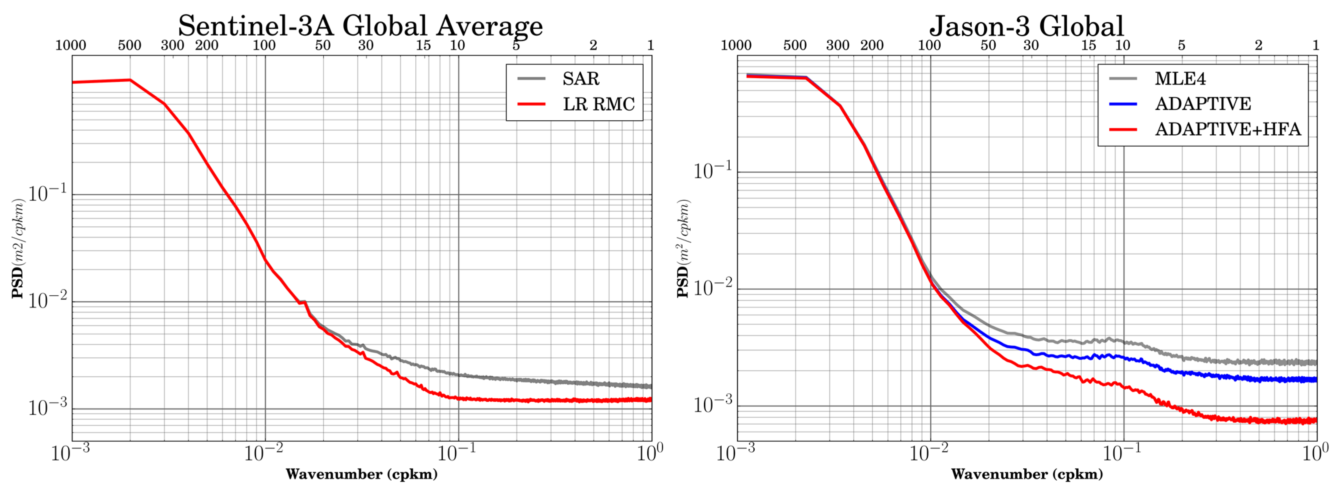
2.2.1. Innovative Processing for Sentinel-3 SAR and Jason LRM

In order to improve the sea-surface height (SSH) observation accuracy, the LR-RMC [27,29] and adaptive [33,47] processes have been used for S3A, J3, and Jason-2 (J2) measurements.
The LR-RMC method is an experimental process developed by CNES. It is close to the current SAR processor. However, it combines the beams produced in a radar cycle differently in order to enlarge the effective footprint of the measurement and average out the effects of the sea-surface state, especially wind waves and swells that are known to impact SAR-mode performance at the short mesoscale (<~50 km). Consequently, the red noise usually observed in the spectrum of SAR sea level anomalies at short wavelengths [59] is reduced, and so is the measurement noise level, which is illustrated in Figure 1. The gray spectrum corresponds to the SAR processor. It has a slightly negative slope, or “red” noise, at short wavelengths (<~50 km). Part of this error signal is assumed to be correlated with swell conditions, as demonstrated by [59]. The red spectrum was generated using the LR-RMC process. In this case, the result obtained is closer to the theoretical spectrum expected, with the noise plateau visible at short wavelengths and the signal’s spectral slope visible at higher wavelengths. A direct impact of this LR-RMC processing is a reduction in the errors at short wavelengths, allowing us to better observe the short mesoscale signal of interest.
The adaptive method is a new retracking algorithm that combines the benefits of four different improvements with respect to the classical MLE-4 (maximum likelihood estimator) retracking algorithm currently used for the official products [60,61]. First, a parameter correlated with the mean square slope of the reflective surface (MSS) was introduced in the model. Its impact is mostly visible in the trailing edge of the echo model and allows a better fit to all types of echoes, from diffuse ones (acquired over the ocean) to very peaky echoes observed over specular regions, such as leads in the Arctic Ocean, or calm lakes and rivers. Second, it directly accounts for the real in-flight point target response of the instrument by numerically convolving its discretized values to the analytical model [47]. Third, a true maximum likelihood estimation method is used, which accounts for the statistics of the speckle noise that corrupts the radar echo. Note that the current method implemented in the official products (up to GDR-E version) is a simple least-squares estimation. The chosen estimation method implemented in the adaptive solution is a geometrical method called the Nelder–Mead algorithm. Finally, the algorithm adapts the width of the window on which the fitting procedure is applied in order to remove spurious reflections coming from nadir directions, in particular when the satellite is approaching coastlines. The many advantages brought by the adaptive algorithms are described by [33,46,62]. In particular, a reduction in the SSH noise level of about 10% is observed.

2.2.2. High-Frequency Adjustment (HFA) and Sea-State Bias (SSB) Correction for Measurement Noise Reduction

The altimeter measurement is contaminated by measurement noise that limits the observability of the mesoscale at wavelengths shorter than about 100 km [15,63,64]. For LRM measurements, the spectral hump, visible on the 20 Hz spectrum at wavelengths ranging from about 10 to 50 km, contains specific noise induced by sea-surface roughness heterogeneities within the 1–3 km diameter altimeter footprint [15].
Another significant source of noise comes from correlations between significant wave height (SWH) and range errors that are inherent to any waveform retracking algorithm [32,36]. These correlations are used to define an HFA correction able to significantly reduce the noise on the SLA signal. The methodology used is described by [35]. It was applied to all the measurements of the different LRM missions, taking into account the specific processing previously described (e.g., adaptive retracking for Jason).
The SSB correction also allows us to reduce the effects of the presence of ocean waves at the surface. A refined 2D SSB solution was used. It was adapted to the selected retracking algorithm data and based on the standard input parameters (SWH and wind speed). The methodology is described by [35]. This SSB solution also contributes to the measurement noise reduction.
This is illustrated in Figure 1 (right), which shows the J3 SLA spectral content when applying different processing methods. The gray spectrum corresponds to the conventional MLE4 processing. The blue spectrum was generated from measurements processed with the adaptive processor combined with the refined 2D SSB solution. It shows a reduction in noise of about 17% compared with the conventional MLE4 processing method, which was mainly visible at short wavelengths (<~50 km). Note that two thirds of this reduction is induced by the adaptive processing, as discussed previously, while one third of the reduction, i.e., about 6%, can be explained by the improved SSB solution. When applying the HFA correction (red spectrum), the energy level is reduced by an additional 26% at short wavelengths. This includes a measurement noise reduction as well as part of the spatially correlated noise visible on the LRM spectral hump [15].

2.2.3. Up-to-Date Tide Corrections

The version of the different geophysical and environmental corrections applied on the conventional L3 1 Hz products available at the time of the L3 5 Hz production is defined as “DT-2018” standards, which are described in [5]. For the L3 5 Hz production, a different version was used for some corrections, especially for the different tide corrections that are applied in the data processing. The version of the corrections retained follow the more up-to-date OSTST recommendations. A large part of these new solutions also corresponds to the standards that are used in the DUACS DT-2021 1 Hz reprocessing, which have been disseminated by the CMEMS since the end of 2021.
The ocean tide correction used in this product was generated with the FES2014b model [51], including the FES2014 tidal load solution.
The internal tide baroclinic signal is removed from the altimeter measurement using the [19] (HRET 7.0) model solution. It allows the estimation of the coherent part of four tidal nodes (M2, K1, O1, S2). This model is defined in deep water and for medium latitudes; elsewhere, no correction is applied.
The polar tide correction is made with the Desay (2015) model taking into account the mean pole location (MPL) corresponding to the 2017 standard, including the mass loss induced by polar ice melt and recommended by IERS. Compared with the MPL 2015 standard used in the DUACS DT-2018 1 Hz product, this change induces large-scale sea level regional biases with a quadrupole structure of about ±1.5 cm amplitude over a short period.

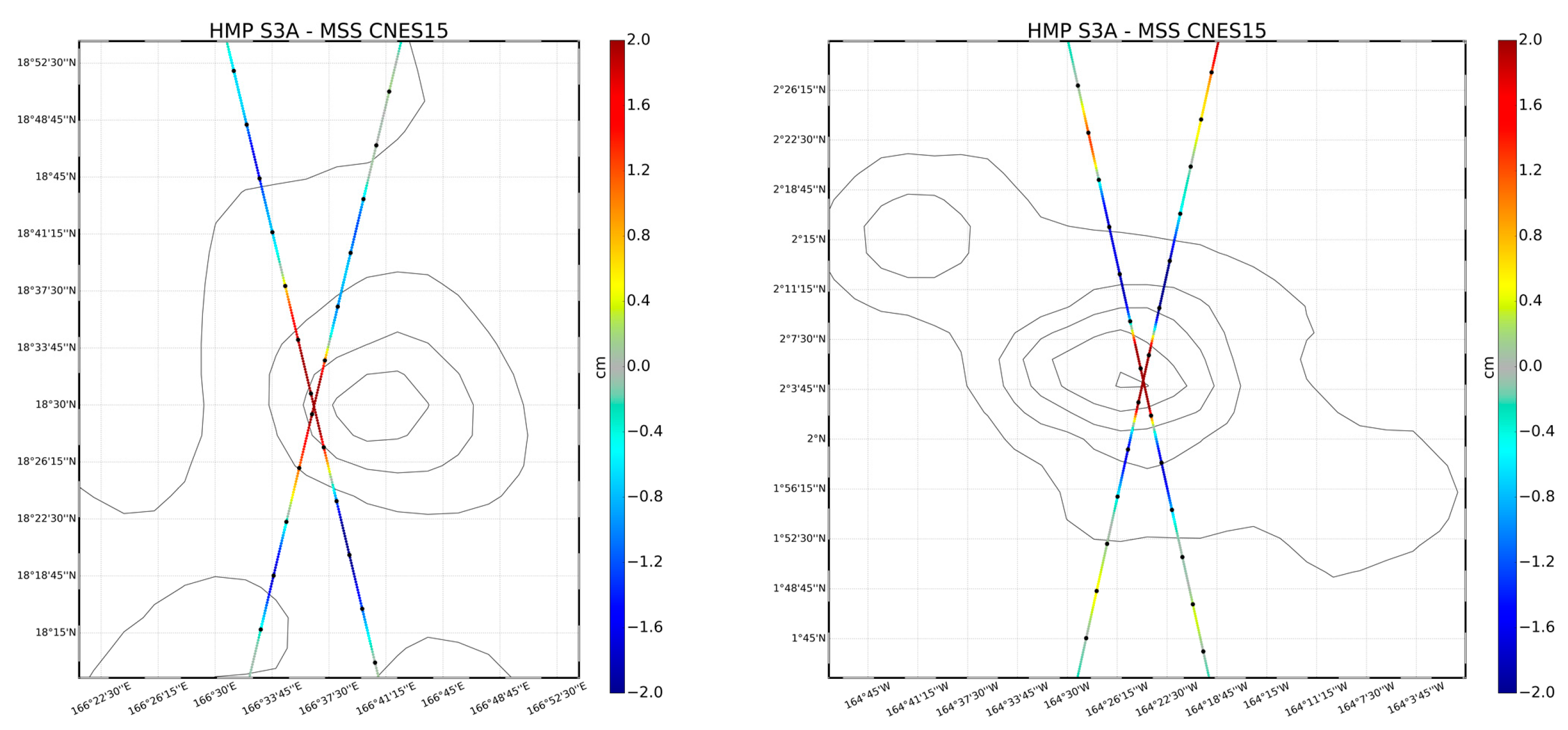
2.2.4. Mean Sea Surface Model

The MSS model used for the SLA computation is the CNES_CLS15 model. It is referenced to the 20-year (1993 to 2012) reference period. This MSS model reduces errors along the repeat tracks that are used for its computation (here, J2 and J3 repeat tracks; [56]). However, errors are higher at the Topex/Jason and ERS/Envisat intertracks, where only a few geodetic measurements were used for the MSS estimation. As this could be a significant limitation for the observability of the short mesoscale signal (<100 km), especially with S3A measurements that were specifically processed to better resolve the small-mesoscale signal, we used a specific MSS [56] for this mission estimated along the tracks of the altimeter, named the hybrid mean profile (HMP). The methodology used for the S3A HMP estimation is similar to the one described by [22]. It includes a specific ocean variability correction to force the 20-year period the HMP should refer to, notwithstanding the limited temporal coverage of the available S3A measurements. The main differences consist of the longer temporal period considered—nearly 2.5 years—and the use of up-to-date altimeter standards and corrections, as described in Table 1. The quality of the S3A HMP was analyzed at short wavelengths using the methodology described by [22]. It has a mean error of 0.12 cm2, i.e., about 10% of the noise-free SLA signal variance. Compared with the CNES_CLS15 reference MSS, the errors are significantly reduced by about 70%. The main reduction in error occurs in the geodetic structures, as previously observed by [22].
The HMP content is illustrated in Figure 2, which shows the differences between the CNES_CLS15 gridded MSS model and the S3A HMP when S3A flew over a small seamount, underlined by the bathymetric contour lines (black lines). The positive anomalies in the HMP–MSS differences correspond to an additional signal in the HMP not present in the gridded reference MSS. Here, the HMP–MSS differences highlight the signature of the bathymetric structure, which is flattened in the gridded reference MSS and more clearly represented in the HMP. The good consistency of the signal observed along both the S3A tracks crossing the structure allows us to have confidence in the representation of this additional signal observed in the HMP. We also note that the seamount signature on the HMP shows up at short wavelengths. The positive values crossing the seamount cover a section about 15–20 km long. This means that such a structure is difficult to accurately capture with 1 Hz altimeter measurements at a sampling rate close to the Nyquist frequency. This also underscores the value in processing the altimeter measurements at a high resolution for a more accurate MSS estimation.

2.3. Valid Data Selection

The valid data selection criteria usually applied for the 1 Hz data processor [65] use parameters that are specific to the 1 Hz products and cannot be applied to the 20 Hz data. Consequently, the valid data selection strategy used for the L3 5 Hz production was reviewed as follows:
As for the 1 Hz processing, the first step is to eliminate all measurements over land. The land–sea flag given in the L2 product is used for this purpose. Ice-contaminated measurements are rejected using the criteria described below. Then, basic threshold criteria on SLA and SWH are used to reject aberrant measurements. Finally, a specific analysis along each altimeter track allows us to reject invalid SLA measurements over the ocean, as described below.

2.3.1. Ice-Contaminated Data Detection

When available in the upstream L2 products, the waveform classification was used to reject ice-contaminated measurements. This criterion was combined with the ice concentration given by OSISAF [66] in order to avoid measurement rejection over open water (ice concentration equal to 0%) and to apply a restrictive selection in high-ice-concentration areas (ice concentration > 50%). The measurements in the medium-ice-concentration areas (ice concentration ≤ 50%) are rejected when the waveform corresponds to a peaky measurement, a sign of potential contamination. This specific data selection criterion was applied on S3A and AltiKa measurements.
For the J2 and J3 measurements, no waveform classification was available, so only the product’s ice flag was used.
For the C2 mission, neither the product ice flag nor the waveform classification were available. Instead, the OSISAF ice concentration was used with a 50% ice concentration threshold criterion.

2.3.2. Open Ocean Data Selection

The valid data selection in the open ocean is based on an iterative kσ editing applied to the SLA and is divided into two steps. At each step, the k coefficient is optimized in order to detect as many invalid measurements as possible while maximizing the availability of valid measurements. The process is applied to each track individually. First, SLA data outliers are rejected according to a k1 σ criterion, σ being the SLA variability along the track considered and k1 depending on the statistical ocean variability at the location considered in order to relax the threshold criterion in high-variability areas (e.g., the Gulf Stream). This avoids a too-severe data rejection in high-variability areas, where intense mesoscale structures could otherwise be rejected. Then, the track considered is iteratively processed in order to reject invalid SLA measurements using a k2 σ criterion applied to the short-wavelength SLA signal dominated by measurement noise. The short-wavelength content of the SLA is extracted using a Lanczos filter, σ is estimated at each iteration, and k2 depends on the SWH signal using the nearly linear relationship observed between the short-wavelength SLA content (dominated by measurement noise) and the SWH for SWH higher than ~2 m. For lower SWH values, k2 is set to the minimal value of three. This avoids a too-severe rejection of the SLA measurements in high-SWH areas, where the noise measurement is usually higher.

2.4. Short Wavelengths Noise Filtering and Signal Subsampling

In spite of the different processing methods and corrections applied, which aim to resolve as much of the short-wavelength signal as possible, the measurement remains significantly contaminated by residual noise. A specific spectral analysis was applied in order to define the observable wavelength for the different missions. The methodology and results are discussed in more detail in Section 3.2. The observable wavelengths were defined in a conservative way, considering the balanced (geostrophic) motion and noise signals. They are presented in Table 2. They range from 35 to 55 km in the North Atlantic area, depending on the mission considered. These values are representative of each mission’s measurement accuracy, and they are used as cut-off wavelengths for the low-pass Lanczos filters applied to the signals. This strategy differs from the conventional DUACS 1 Hz processing for which a unique, mean cut-off wavelength is used to low-pass filter the measurements, whatever the mission.
The measurements are then subsampled in order to be consistent with the observing capabilities. A final 5 Hz sampling, i.e., slightly more than 1 km between two consecutive measurements, was retained as a good compromise between the sampling needs and observing capabilities.

2.5. Long-Wavelength Error Correction

The LWE correction is the final step for the homogenization of the multi-mission signal. Its purpose is to reduce the regional discrepancies observed between neighboring altimeter tracks. These biases are induced by, among other things, residual orbit and geophysical or environmental correction errors. For both DUACS 1 Hz and 5 Hz processing, the LWE is estimated by a two-step procedure: (1) a sparse estimation of the LWE correction along the track made by optimal interpolation (OI); (2) the sparse estimation interpolated at each along-track measurement location.
There are, nonetheless, some differences in how the procedure is implemented for 5 Hz data. First, for step one, the sparse estimation of the LWE correction along the tracks of the altimeters is performed using a 100 km sampling rate instead of the 500 km rate usually used in the DUACS 1 Hz processing. Then, for step two, an OI method is used to interpolate the LWE correction on each individual 5 Hz measurement location, whereas the 1 Hz processor uses cubic spline adjustment, as described by [1]. This OI approach allows us to finely tune the cut-off wavelength that needs to be estimated for the LWE signal, typically of the order of 2000 km. Additionally, so as to account for the different dynamics of semi-enclosed seas, the different passes are split into independent segments when overflying land. This improves the LWE correction and its ability to correct the residual errors caused by a reduced quality of the various geophysical, atmospheric, and environmental corrections.
An example is given in Figure 3. It shows the mean LWE correction computed for C2 1 Hz measurements in 2014, comparing the DUACS 1 Hz processing (left) and the updated methodology defined for the 5 Hz processing (right). When applying the DUACS 1 Hz LWE processor, the correction obtained does not show any specific geographical pattern that can be correlated with a physical signal. On the other hand, the LWE correction obtained when applying the processor defined for the 5 Hz production shows a more structured signal, with positive and negative values (up to ±1 cm) aligned along the magnetic equator. This pattern evokes an ionosphere-related signal, highlighting the imprecision of the global ionospheric model correction for this mission due to the lack of dual-frequency altimeter measurements.
We used statistics at cross-overs in order to quantify the impact of the LWE correction applied. Indeed, as the LWE correction acts to reduce the residual long-wavelength biases observed between neighboring tracks, it also reduces the variance in the SLA differences at cross-overs. Table 3 shows the mean variance in SSH differences at cross-overs for the global ocean over a one-year period for J3. Mono-mission (J3/J3) and multi-mission (J3/Sentinel-3B (S3B)) cross-overs are considered. Here, only J3 is corrected for the LWE, while S3B is not used for the LWE estimation and thus remains independent. Statistics obtained when not applying the LWE correction, when applying the LWE correction deduced from the conventional DUACS 1 Hz processing, and from the 5 Hz processing, are given. They show that the LWE correction obtained with the Duacs 1 Hz processing significantly improves the consistency of the SLA between tracks and removes discrepancies at cross-overs, with a 1.5 to 2 cm2 reduction in variance. The results are further enhanced when using the LWE method defined for the 5 Hz processor, with an additional 1 to 2.5 cm2 reduction in variance, i.e., an additional improvement of 9 to 15% for multi-mission and mono-mission cross-overs, respectively, compared with the previous LWE version. The improvement is higher at mono-mission cross-overs when both the tracks are corrected (while only J3 tracks are corrected at multi-mission cross-overs).

2.6. Across-Track Current Estimation

The geostrophic velocities in the across-track direction were estimated using a centered difference method with two measurements on either side of the point considered.

3. Data Validation

Although five different altimeter missions have been processed, the validation of the product presented in this paper mainly focuses on the S3A and J3 missions. The former is representative of the SAR technology, while the latter is representative of the LRM measurement. Moreover, significant evolutions have been implemented on these two missions, as discussed in Section 2.1.
The data were assessed in terms of data availability, spectral content, and consistency with independent tide gauge measurements. They were also compared with the 1 Hz product available on CMEMS (produced in accordance with the DUACS DT-2018 standards).

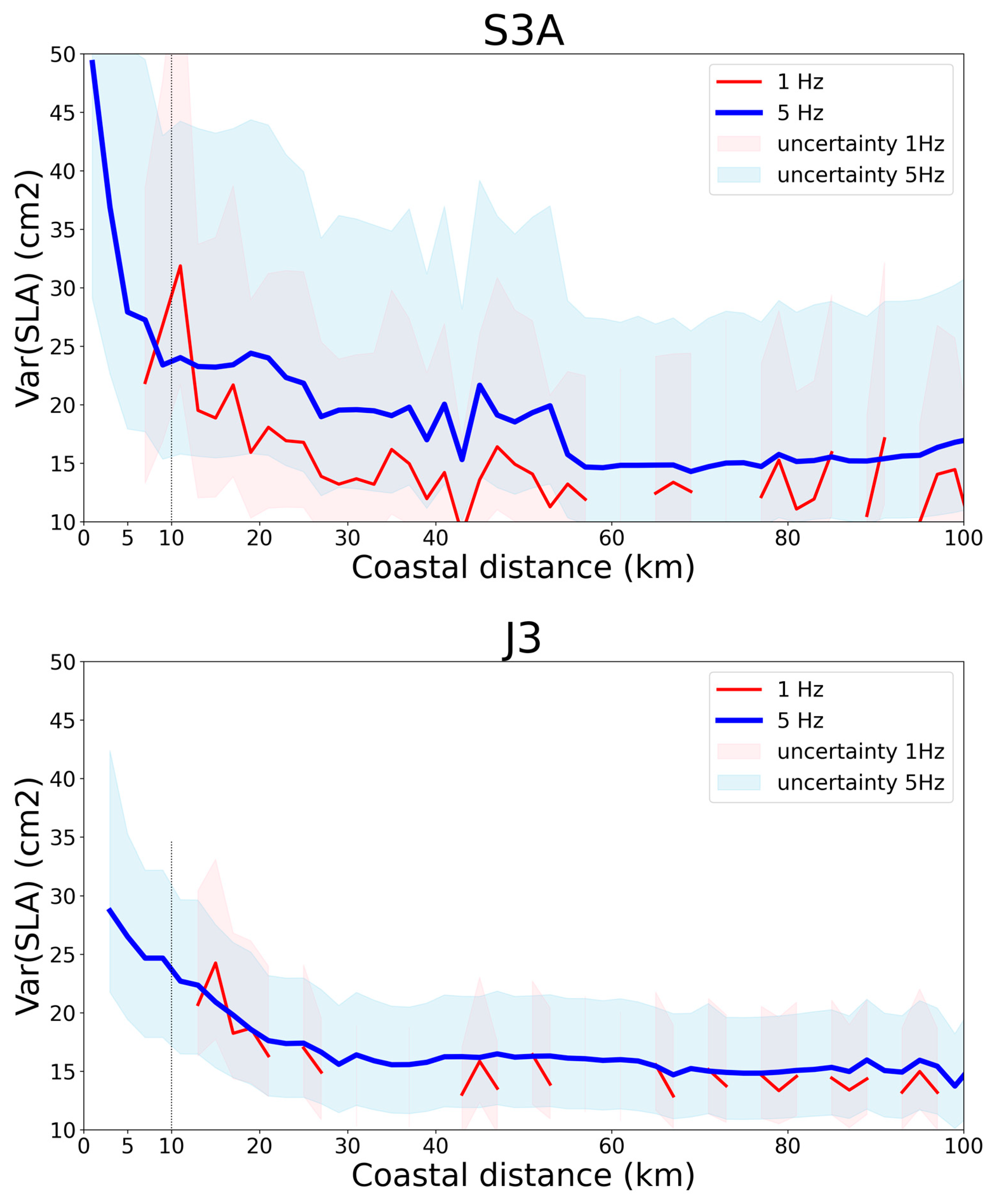
3.1. Data Availability and Gain Brought by the 5 Hz Altimeter Processing near the Coast

The processing used for the valid data selection can have a significant impact on the data availability rate. In the L3 5 Hz processing, the data selection strategy aims to optimize the rejection of the measurements retained as invalid without greatly reducing the data availability rate (see Section 2.2). An example of the rate of rejected measurements obtained is illustrated in Figure 4 (left) for the SAR mission (S3A) and the LRM mission (J3) for January–April 2018.
For both missions, the most drastic rejection occurs in the ice-contaminated areas. Indeed, the processing applied mainly focuses on the open ocean and is not adapted to the possible measurements available over leads. As described by [45], the observation of the SSH in such narrow ice-free areas requires a specific delay-Doppler processing method not implemented here. Consequently, no efforts have been made to keep the measurements over leads.
Within a band extending from 5 to 10 km from the coast, there is a high rate of data rejection of more than 30%; this increases to over 60% within 5 km from the coast. In the open ocean, the rejection rate drops to between approximately 0.5 and 1% of the available measurements. We observe here that the rejection rate remains homogeneous in the open ocean. This is noteworthy: In the region depicted and for this season, the SSH measurements are sensitive to high SWH (see for example [65]), but the optimized data selection strategy used in the full-rate processing takes into account the higher measurement noise in these areas, reducing the rejection rate in areas of high SWH (see Section 2.2).
Although they are not directly comparable due to the different sampling rates, we nevertheless observe that the valid data availability in this demonstration product is overall higher than for the conventional 1 Hz product, especially in coastal areas. Table 4 shows statistics of the mean distance of the nearest point to the coast for which the sampling rate reaches at least 80% of the maximum number of cycles defined for the period between mid-2016 and the end of 2018. All tracks’ extremities are considered over the European coasts. They show that, in the mean, the conventional 1 Hz product is defined up to 10 km to the coast for the SAR mission S3A and 11 km for the LRM mission J3, while this distance is nearly half as long for the 5 Hz product, with about 5 and 6 km, respectively.
In order to assess the pertinence of the measurements retrieved near the coast, we analyzed the SLA variance when approaching the coast. Figure 5 shows the evolution of the mean SLA variance over the northern Spanish coast as a function of the distance from the coast for J3 and S3. Only measurements with a minimal availability rate of 80% across the whole time series are considered. Statistics are computed using 2 km wide bands of distance from the coast. The restricted coastal area was selected for its nearly uniform ocean dynamics, and thus avoids mixing different dynamic regimes.
We first note that, especially for the J3 mission, the data availability near and even far from the coast is degraded when using the 1 Hz product. This explains the discontinuities in the statistical plots for the 1 Hz product. The reduced availability of the 1 Hz product is caused by the more severe data selection criteria applied, as discussed before. The lower sampling rate is also a factor, since with a distance of nearly 7 km between consecutive measurements, and with a restricted number of passes in this area (five passes), there is a lower likelihood of filling all the coastal distance bins. We also see that for both J3 and S3A, the SLA variance level is slightly higher for the 5 Hz product than the 1 Hz. For J3, it reaches 15.3 cm2 for the 1 Hz and 16.3 cm2 for the 5 Hz product. For S3A, it reaches 14.7 cm2 for the 1 Hz and 17.9 cm2 for the 5 Hz product. This is explained by the different cut-off wavelengths used for the signal filtering, ranging from 35 km for S3A to 55 km for J3 at 5 Hz (see Section 2.3), and 65 km at 1 Hz. We note, however, that the difference remains low when considering the different noise levels in the upstream products used (i.e., noise variance is reduced by a factor of 20 in the 1 Hz upstream product compared with the 20 Hz due to the 1 Hz compression). This result is made possible by the innovative processing applied for these two missions (see Section 2.1), significantly reducing the noise level for the 20 Hz measurements.
The evolution of the SLA variance is stable down to nearly 30 km from the coast for both missions at both resolutions. Then, it starts to increase when approaching the coast. The increase is regular and homogeneous for J3, both at 1 Hz and 5 Hz sampling rates. While no measurements are available for the 1 Hz product within 12 km of the coast, for the 5 Hz product, the SLA variance continues to increase at the same rate as the signal observed further offshore. The variance reaches nearly 30 cm2 near the coast. For the S3A mission, the 1 Hz product also reveals a nearly linear increase in SLA variance when approaching the coast. This product does not allow an accurate sampling of the signal within 5 km of the coast and there is a suspicious peak of SLA variance at around 10 km from the coast. This peak is not seen in the 5 Hz product. The latter rather features a nearly linear increase in SLA variance down to ~5 km from the coast, consistent with what was observed with the J3 mission. In the last five kilometers, the SLA variance increases sharply to reach nearly 50 cm2 close to the coast.
The evolution of the SLA variance suggests that the quality of the retrieved signal is better with the 5 Hz product, especially within ~12 km of the coast, where there are no 1 Hz data. However, while various physical signals can contribute to a higher variance in the coastal area (wind–waves, trapped waves, currents, etc.), the sharp increase in variance observed with S3A in the last five kilometers rather suggests residual errors, meaning that the 5 Hz products should be used with care within ~5 km of the coast.

3.2. Observing Capability

The SLA power spectral density (PSD) analysis was used to define the minimum wavelength associated with the dynamical structures that altimetry would be able to observe with a signal-to-noise ratio (SNR) greater than 1. The methodology was derived from [63] and consists of finding the wavelength for which the SNR is equal to 1, the signal being defined by the mesoscale spectral slope and the noise by a constant value fitted to the spectral plateau (or nearly flat slope) visible at the shortest wavelengths or on the residual spectral hump when its signature is well defined. The determination of the spectral slope and noise is performed by least-squares fitting a two-line sum model to the signal PSD. The observing capability was defined over the northeast Atlantic area ([10, 35°W] [30, 65°N]), in order to be representative of the area of primary interest to the CMEMS community, which allows a selection of sections of tracks long enough to obtain an accurate spectral slope estimation. The full-rate measurement (20 or 40 Hz) was used in order to better observe the residual noise signature. The results obtained are summarized in Table 2. They are representative of the mean value over a 1-year period.
The observing capability estimated with the full-rate product processed as described in Section 2 ranges from 35 to 55 km according to the mission. As expected, the observing capability is smaller for S3A. This capability is explained by the use of SAR technology [67] combined with LR-RMC processing [27] that [29] applied to this mission. C2 and ALG should be able to observe up to 40 km. For C2, the presence of the SAR-mode measurement in a large part of the area considered, combined with the HFA correction for LRM-mode measurement, explain this result. The Ka band used for the AltiKa mission, which has a lower noise level than the Ku band used for other LRM missions [24], combined with the HFA noise reduction processing [35], enables it to observe the small mesoscale. Finally, the LRM Jason missions should observe wavelengths longer than 55 km. The slightly degraded observing capability for these missions is caused by a higher sensitivity of the measurements to the sea-surface inhomogeneities producing a well-defined spectral hump [15], thus contributing to a higher noise level in the measurements, especially during the winter time, notwithstanding the HFA correction applied.
In order to be compared with the 1 Hz products’ observing capability, the same methodology was applied to 1 Hz measurements currently available from the CMEMS and processed with the conventional DUACS system. The S3A mission, representative of SAR technology, and the J3 mission, representative of LRM technology, were compared. The results are also summarized in Table 2. They show that in the North Atlantic, the conventional 1 Hz sampling allows the observation of wavelengths longer than about 65 (S3A) or 85 km (J3). In other words, the full-rate processing applied here reduces the observable wavelength by nearly half for the SAR mission (S3A) and by one third for LRM measurements (J3). In the case of the S3A measurements, the reduction in the observable wavelength observed here is greater than the mean reduction reported by [29] when comparing the performances of SAR vs. LR-RMC full-rate processing. The authors indeed reported a reduction of nearly 1/3 of the observable wavelength with LR-RMC compared with the SAR processing. However, in the present study, we do not directly compare SAR (here in 1 Hz) vs. LR-RMC (here in 20 Hz); instead, we compare the capabilities of two different product lines, thus including differences in the processing strategy, i.e., differences in the retracking mode, as in [29], in addition to differences in the corrections and data selection. In this case, the performance of the full-rate measurement is strongly linked to the area considered and cannot be extrapolated as a global mean performance. Indeed, the presence of high SWH in the North Atlantic region significantly increases the noise in the processed SAR and MLE4 measurements and thus reduces their observing capability. In the case of the 20 Hz measurement, this effect is counterbalanced by the different processing methods discussed above (i.e., LR-RMC and adaptive + HFA processing).
Although the wavelengths presented in Table 2 have been used as cut-off wavelengths for low-pass filtering over the whole North Atlantic area (see Section 2.3), they are not fully representative of the observing capability over the different sub-regions and seasons. Over enclosed seas, the reduced SWH, which results in lower noise levels, combined with the smaller mesoscale signal usually observed in such regions, should improve the observing capabilities for the different altimeters. An SNR equal to 1 has been estimated over the Black Sea region for SAR missions (S3A and C2) processed for a specific ESA project (EO4SIBS [68]). The results suggest that these measurements should enhance the observability of wavelengths up to about 25 to 30 km in this area (not shown). In the same way, seasonal modulations of the mesoscale activity, mainly driven by the seasonal variations in the mixed-layer depth [69], reduce the mesoscale spectral slope in winter. At the same time, higher SWH and higher sea-surface inhomogeneity contribute to an increase in the residual noise level. As a consequence, seasonal variability in the observing capability can be observed, as previously reported by [63,70].

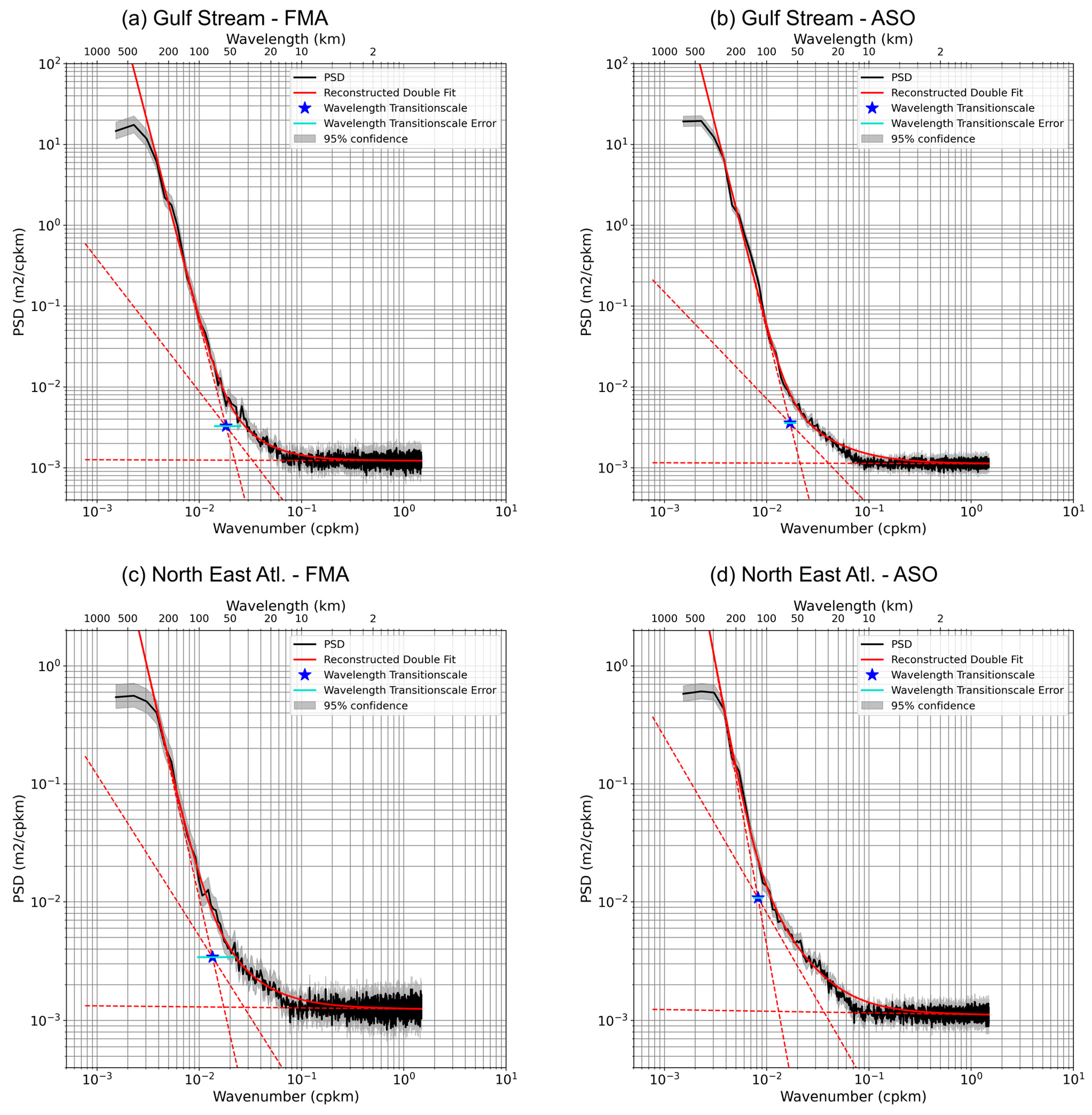
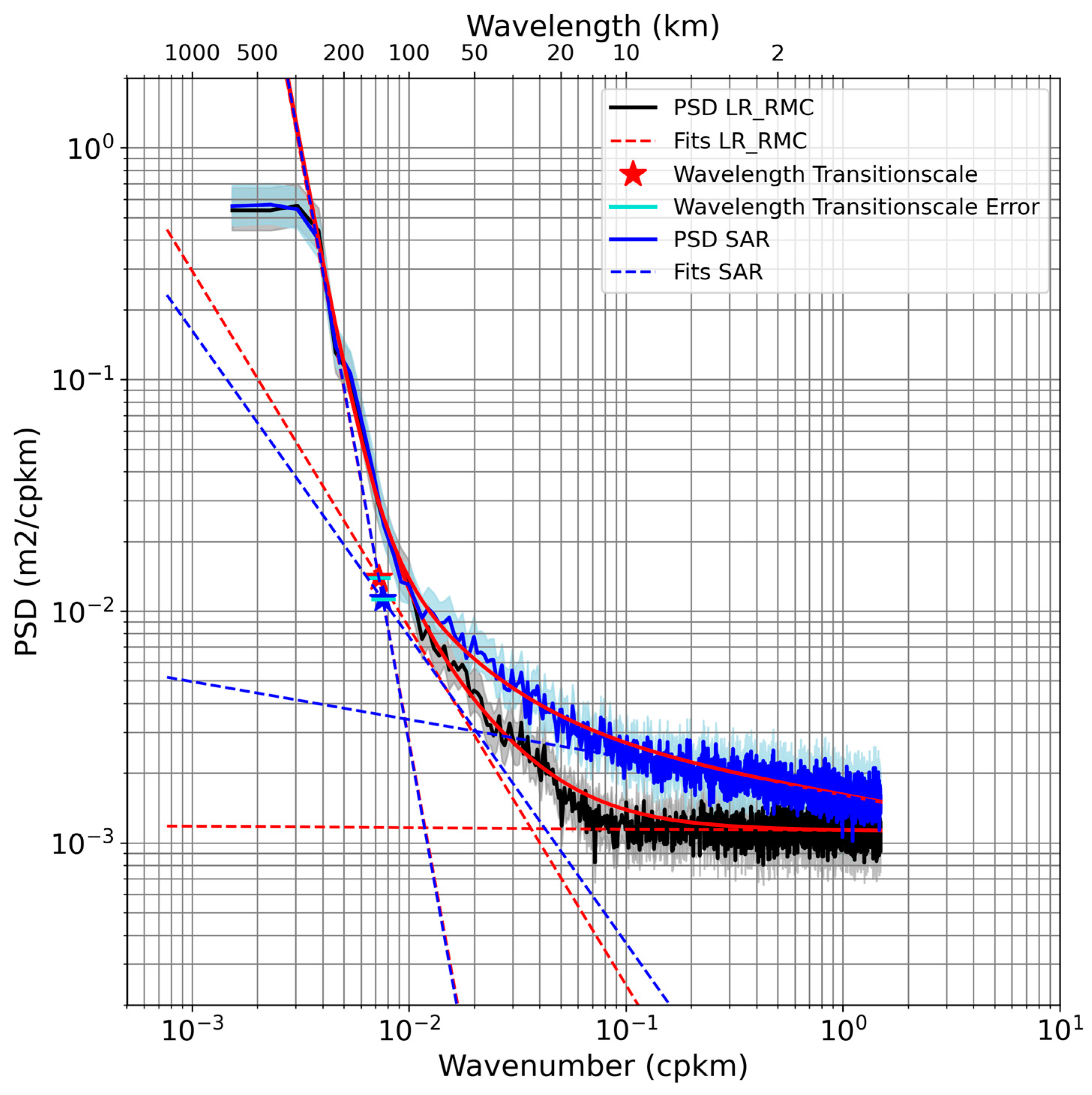
3.3. New Insight into the Altimeter Spectral Content with Sentinel-3A

In recent years, high-resolution models combined with in situ measurements have given us new insights into ocean dynamics at short wavelengths. Several studies [11,69,71] have underlined the importance of the unbalanced motions that contribute to the energy cascade and dissipation at these wavelengths [11,72]. Combined with the balanced motions, they thus significantly contribute to the shape of the kinetic energy spectrum and the SSH spectral slope at wavelengths lower than ~150 to than 50 km or less, depending on the area and the season [71]. While only a few years ago the high noise level in altimeter measurements prevented us from being able to access these wavelengths, progress in altimeter measurement now leads us to revisit the analysis of the SLA spectral content. Additionally, recent work from [70,73] proposed a refined methodology for a more accurate SLA PSD analysis. Here, we adapt the methodology to analyze the spectral content of the S3A measurements. Indeed, the low noise level of the SAR measurements and LR-RMC processing makes S3A the best candidate to explore the sea-surface dynamics at short wavelengths.
As before, the full-rate (20 Hz) measurements are used in order to access the full spectral content. Although LR-RMC processing significantly reduces the measurement errors linked to swell [29], only measurements associated with low SWH (below 4 m) have been considered in order to avoid the possible contamination of the signal with residual errors. The SLA PDS has been analyzed over two different areas: the Gulf Stream core, and a less energetic area located further east in the Atlantic Ocean (precise coordinates are given in Table 5). The mean SLA PDS over the years 2017 and 2018 and for the winter (February–March–April; FMA) and summer (August–September–October; ASO) seasons have been analyzed. The spectral decomposition used is similar to the one proposed by [73]. It consists of first estimating the noise level—represented by the flat signal at the shorter wavelengths (<10 km)—then the slope characterizing the geostrophic or mesoscale signal—usually well-defined at wavelengths > ~150 km—and a second slope expected to be representative of the unbalanced motion visible at the small mesoscale. Mesoscale and small-mesoscale slopes are fitted on the noise-corrected PDS using a two-line sum model. The results obtained are presented in Figure 6 and show the mean PSDs for the regions and seasons considered. The black line represents the true PSD deduced from the altimeter measurements. The 95% confidence interval is represented by the light gray band centered on the true PSD. The three slopes deduced from the spectral decomposition are shown as dashed red lines. The thick red line shows the theoretical spectrum deduced from the sum of the three different slopes. Finally, the transition scale (Lt) defined for where the mesoscale (balanced motion) to small-mesoscale (unbalanced motion) signal ratio is equal to 1, is represented by the blue star. Details of the characteristics of the different PSDs are given in Table 5.
The results regarding the geostrophic dynamics are consistent with those reported by previous studies [70]. They feature dynamics close to QG (quasi-geostrophic) theory (spectral slope close to K−5 [64] in the Gulf Stream). The spectral slope is reduced and rather close to the SQG (surface QG) theory in the northeast Atlantic area, especially in winter (spectral slope close to K−11/3). The seasonal variability is well pronounced in this latter area, with a net deepening of the slope in summer (K−4.7) linked to the less intense mesoscale activity at short wavelengths in this season, which in turn is connected to the characteristics of a shallower mixed-layer depth (MLD).
The slope observed at the small mesoscale is flatter than the slope of the balanced motion. It ranges from K−1.32 to K−1.64 according to the region and season considered. These values are in accordance with unbalanced motion or internal gravity wave (IGW) dynamics that are expected to have a SLA PSD slope close to K−2 theory [74]. Finally, the transition between balanced and unbalanced motion is found to range from ~50 to 120 km. A mean Lt of about 53 km is observed over the Gulf Stream core, with relatively low seasonal variability (55 km in winter and 59 km in summer). In contrast, Lt observed in the northeast Atlantic domain is strongly seasonally variable with minimal values around 75 km during the winter period and a maximal value around 120 km during the summer period. Although the estimation error of the Lt remains high (up to 56 km in summer in the northeast Atlantic), the results obtained are coherent with the unbalanced motion that is enhanced by a shallow MLD and strong pycnocline observed in summer [11]. The results obtained in characterizing the unbalanced motion are also consistent with those reported by [71]. The authors used a numerical model to estimate the Lt wavelength. They reported values of about 50 km in the Gulf stream and slightly more in the northeast Atlantic, with significant seasonal variability. The analysis of the results over the single-year seasons also suggests interannual variability in the balance between balanced and unbalanced motions. The greatest variations were observed during the winter months for the northeast Atlantic box. In this region the signature for unbalanced motion is well defined for winter 2017. Over this period, it dominates over the geostrophic and noise signals at wavelengths ranging between about 70 and 30 km. However, during winter 2018 balanced motion seems to dominate the signal up to wavelengths of about 50 km. In this case, the residual measurement noise does not allow us to extract the signature of the unbalanced motion for this domain/period (no shown).
The variability explained by the unbalanced motion remains low, especially in the Gulf Stream or during the winter period. For that area and season it dominates the noise and mesoscale signals over a short 20 to 30 km wavelength band (see Figure 6a for instance). In these conditions, the observability of this signal remains limited when considering measurements that have not been optimally processed to reduce the errors at short wavelengths. This is the case with conventional SAR measurements. Indeed, with higher level, red colored noise, affecting the signal at wavelengths up to ~50 km (as visible for instance in Figure 1 over the global ocean), the SAR measurement errors mask most of the unbalanced motion in areas and seasons where this component is low. Elsewhere, SAR measurement capabilities still allow us to resolve part of the unbalanced motion. In this way, the high-resolution SAR measurements were used to estimate the SLA spectral content over the northeast Atlantic area during the 2017 summer period. The corrections applied to the SAR measurements are consistent with those used in the LR-RMC processing described in Section 2.2.1. Results obtained with SAR- or LR-RMC-processed measurements can be seen in Figure 7. Both the processing methods show similar results in the Lt estimation, with 137 km obtained with LR-RMC and 132 km with the SAR. However, the sub-mesoscale spectral slope estimated with SAR remains flatter (K−1.32) than the one deduced from LR-RMC (K−1.54). The latter is closest to the theoretically expected K−2 slope [74]. It is clearly apparent in Figure 7 that the red noise affecting the SAR measurements dominates the signal at wavelengths shorter than 50 km, and the lower level of noise achieved with the LR-RMC processing allows us to resolve the signal up to about 30 km (SNR = 1 considered). This leads to the lower accuracy of the unbalanced motion observation with the SAR processing. In the same way, the high-resolution measurements, optimally processed to reduce errors at short wavelengths, add a higher precision in the characterization of the unbalanced signal. However, ref. [73] showed that part of this signal can be recovered with conventional 1 Hz measurements. In this case, a long temporal period is used in order to reduce the errors during the estimation.

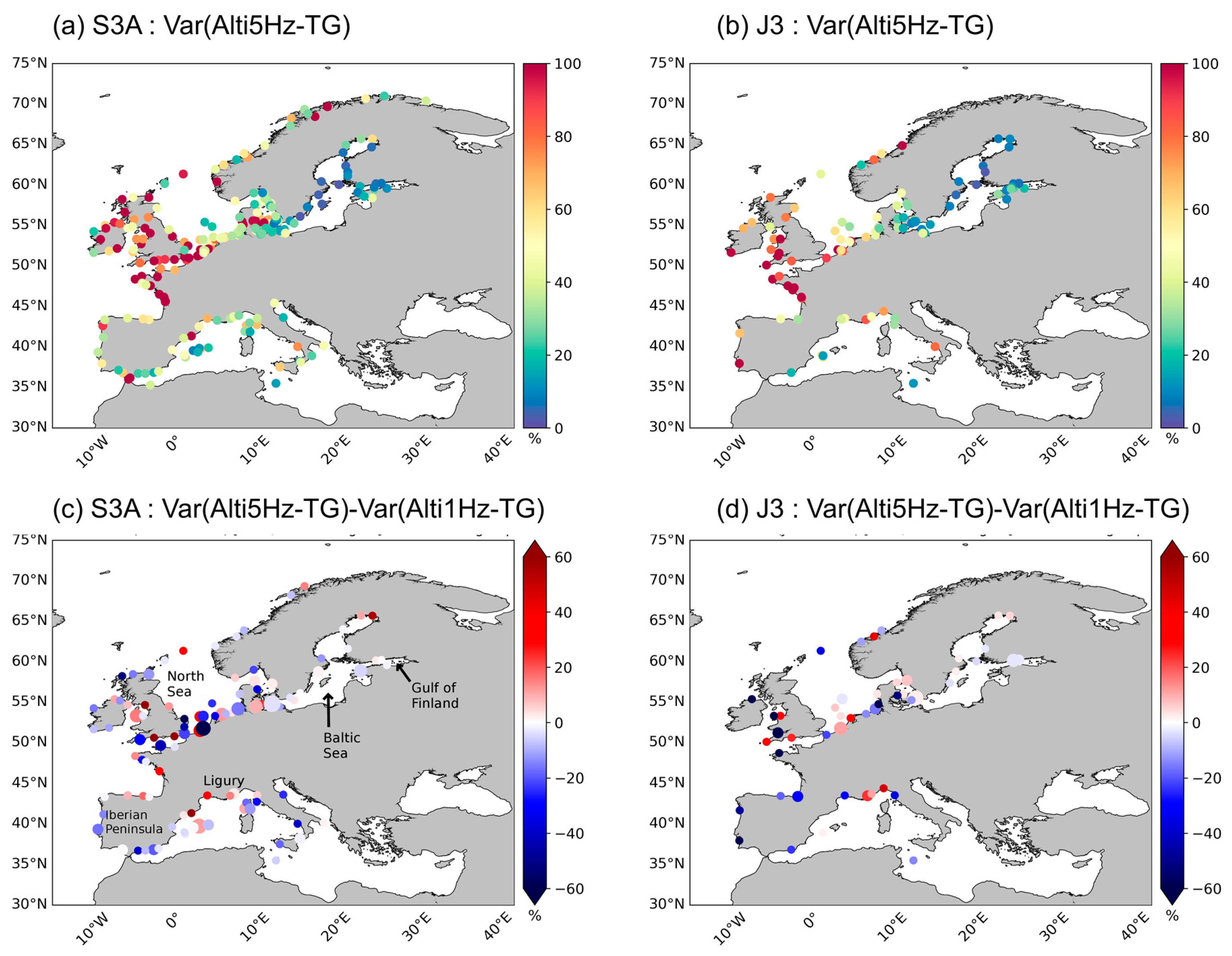
3.4. Consistency with TG

The dense tide gauge (TG) network provided by the Copernicus Marine Service (CMEMS) over European waters was used to assess the quality of the altimeter measurements. The methodology used is derived from the one described in [75] and can be summarized as follows: First, TG series with anomalous events or with significantly higher variance (more than 20 cm2) than the altimeter data are rejected. Then, selected TG series are processed in order to obtain an SSH signal comparable to the altimeter measurement content. The tidal signal is removed using a harmonic decomposition proposed by [76]; the dynamical atmospheric signal [17], also corrected for in-altimeter measurements, is removed from the TG signal. To do so, the TG series are first converted into 6-hourly records; vertical motions linked to the post-glacial rebound are also removed from the TG signal using the Peltier model [77,78]. After that, TGs and altimeter measurements are collocated using the maximal correlation score within a 25 km area around the TG stations. Note that this distance is reduced compared with the one used in [75] (i.e., ~100 km) in order to better focus on near-coast measurements. The next step consists of rejecting time series less than 10-months long to guarantee statistical significance. Finally, global mean statistics are computed. With the aim of reconciling the different spatial sampling capabilities between the TG network and the altimetry, different weights were used for the different TG stations selected. The weights depend on the number of neighboring TGs (a maximal distance criterion of ~100 km was used), which are compared with an altimeter measurement and aligned along the same altimeter ground track. This processing was applied to S3A and J3 1 Hz and 5 Hz products. A filtered SLA signal, as disseminated in both 1 Hz and 5 Hz altimeter products, was used. The results are compared for TG stations that are common to both altimeter products. The data were compared over the period from July 2016 to September 2018.
The results obtained for S3A and J3 are consistent. They are presented in Figure 8, which shows the variance in the differences between altimetry and TG signals when using the 5 Hz altimetry product for S3A and J3 (top), as well as the differences with the results obtained when using 1 Hz altimeter products over the common TG stations selected (bottom). Results are expressed as percentages of the TG signal.
The TG selection criteria allowed us to select 232 TG sites for the comparison with S3A and 99 sites with J3 5 Hz altimeter products, i.e., respectively ~63 and 27% of the initial number of the TG available. They are located along the main part of the European coasts, except in the Black Sea and western Mediterranean Sea. The mean distance between the TGs and the altimeter measurements selected is around 20 km for both of the altimeter missions. The variance in the differences between the altimeter and the TG measurements shows a spatial distribution close to the observation reported by [75] when using CMEMS 1 Hz altimeter products, except that values observed here are slightly higher due to the restricted area used for the altimetry and TG measurement colocation, as discussed before. The lower variances (globally < ~15%) are located in the Baltic Sea, while higher values (>50%) are located in the North West Shelf area.
The number of TG stations retained that were statistically comparable with the altimeter measurements are higher for the 5 Hz product. Indeed, an additional 75 stations are selected with the 5 Hz S3A product, i.e., ~+48% compared with the number of stations selected when using the 1 Hz altimeter product. For J3, an additional 30 stations are selected (i.e., +43%). They are mainly located in the North Sea, Gulf of Finland, Baltic Sea, or in the jagged western UK coasts (not shown). This is due to the higher availability of 5 Hz measurements in coastal areas, as discussed in Section 3.1.
Finally, only 142 and 62 TG stations have been used to compare the respective performances of the 5 Hz and 1 Hz altimeter products for S3A and J3 respectively.. They correspond to the common TG stations selected for both products. The mean statistics observed for the common TG stations are given in Table 6 and Table 7, while Figure 8 (bottom) shows the reduction in the variance in the difference between altimetry and the TG signal when using a 5 Hz altimeter product rather than a 1 Hz product. The results show that the mean distance between the TG and the altimeter’s most correlated point for 1 Hz and 5 Hz altimeter products is nearly the same (~20 km). Nevertheless, the length of the altimeter/TG data pair series is generally longer for the 5 Hz altimeter product, with 8.7% additional pairs for S3A and 5.7% for J3 compared with the results obtained with 1 Hz altimeter measurements. Here, again, this is due to the enhanced data availability of the 5 Hz product near the coast. We also observe in Table 6 and Table 7 that the altimeter signal retrieved with the 5 Hz product is overall more consistent with the TG signal. Indeed, the 5 Hz SLA shows a mean variance in the signal (126 cm2 for S3A; 131 cm2 for J3) close to the mean variance in the TG signal (134 and 154 cm2, respectively). The mean variance in the differences between altimeter and TG signal reaches 58 cm2 for S3A and J3, i.e., between ~43% (S3A) and 38% (J3) of the TG signal. It is reduced by about 17% for J3 to 5% for S3A when compared with the results obtained with altimeter 1 Hz product. This reduction is however not homogeneous in space (Figure 8). It shows well-defined areas where the 5 Hz altimeter product better compares with TG measurements. This is the case for instance along the west and south Iberian coasts or along the Italian coasts. On the other hand, the 1 Hz product for S3A performs better along the Ligurian coast and north Iberian coast. Along the northern European coasts, the 5 Hz product is closer to the TG signal in most TG locations. However, neighboring TG locations can have very different results, especially along jagged coasts.

4. Use Cases

4.1. Assimilation in Numerical Models

The 5 Hz altimeter products have been designed to serve the CMEMS community and more specifically the Model Forecasting Centers (MFCs) that contribute to the CMEMS. The demonstration 5 Hz product was thus proposed to different MFCs for testing, with the main objective to demonstrate the added value of a higher spatially resolved altimeter product for regional models. They used this product for assimilation in regional models in comparison with the results obtained with the assimilation of the conventional 1 Hz product (CMEMS SEALEVEL_EUR_PHY_L3_REP_OBSERVATIONS_008_061 regional product line corresponding to the DUACS DT-2018 standards). In order to avoid biased results, possibly resulting from the improved quality of the signal induced by the different instrumental and geophysical corrections applied in the 5 Hz processing (see Section 2.1), an intermediate version of the demonstration product was used for this exercise. It was constructed using altimeter standards close to the corresponding 1 Hz products available in the CMEMS, and for the revised processing method, only the HFA correction, which is necessary to significantly reduce the error at short wavelengths, was applied in the L3 5 Hz processing for this comparison.
An example of the results obtained with the 1/36° × 1/36° Iberian and Bay of Biscay (IBI) model is fully described by [79], which we summarize here. The authors showed that the assimilation of the 5 Hz SLA reduces the RMSE of the differences between the model forecast and altimeter SLA along the J3 tracks. They report a reduction of nearly 9% of the RMSE compared with the assimilation of the conventional 1 Hz product. However, this result can be improved when the assimilation scheme is enhanced by fully exploiting the variables delivered in the 5 Hz altimeter product. Thus, using the DAC, ocean tide, internal tide, and LWE corrections to adjust the altimeter content to the SSH resolved by the model, a larger reduction in the RMSE can be obtained. The authors report a reduction of 11 to 14% depending on the region. The best scores are in areas where the DAC and tide signals are significant. At the same time, the surface currents resolved by the model when assimilating the 5 Hz rather than the 1 Hz altimeter measurements are more consistent with independent observations from high-frequency radar [80], with a 15 to 20% reduction in the RMSE differences. There was no impact on the consistency between the model SST or T/S profiles and independent satellite or in situ observations.

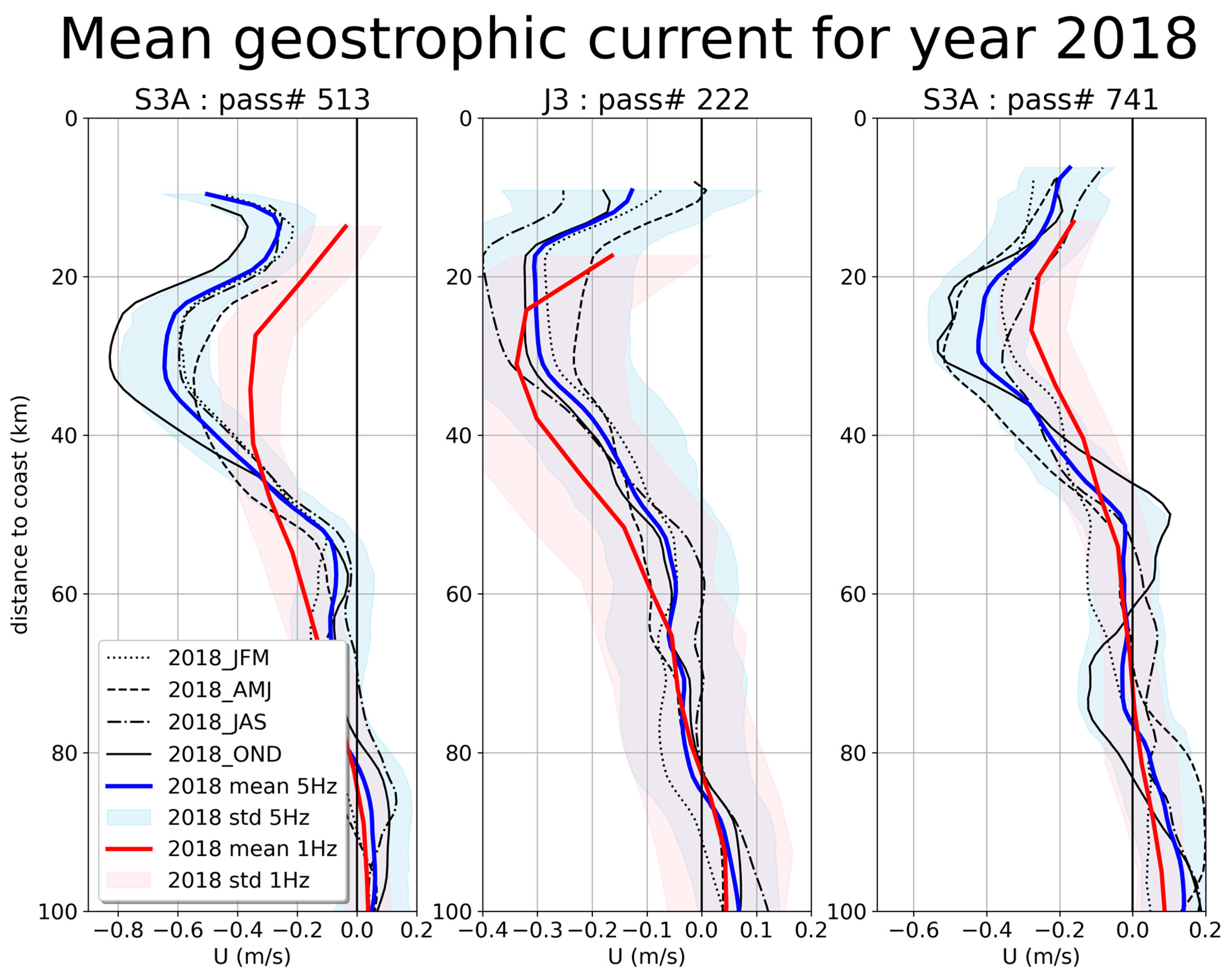
4.2. Coastal Currents

The demonstration 5 Hz L3 products can be used in studies of ocean dynamics and more particularly ocean circulation. We take here the example of the Northern Current (NC) in the western Mediterranean Sea. The J3 track #222 is well known to be optimally positioned to sample the narrow surface boundary NC flowing along the coast from Italy to Spain. At the same time, it crosses a challenging area for altimetry since it is located over a narrow and uneven shelf. This track was widely used in previous studies as for instance by [40,42,81]. For comparison, the signal along the tracks S3A #513 and #741 was also considered. The track #513 is located ~0.5° west of the J3 track, just east of La Valette island, and is optimally positioned to catch the NC over an area where the continental slope is narrow. In contrast, the track #741 is located east of the J3 track and crosses the NC off the western Italian coast, around 7.9°E.
The mean geostrophic current from 2018 was analyzed from both 5 Hz L3 altimeter products presented in this paper, as well as a contemporaneous 1 Hz product available from the CMEMS (SEALEVEL_EUR_PHY_L3_REP_OBSERVATIONS_008_061 regional product line corresponding to the DUACS DT-2018 standards). In the case of the 5 Hz product, the mean current was directly computed as a temporal mean of the total current, i.e., composed of the anomaly of the geostrophic current and mean absolute current both delivered in the product (i.e., mdt_velocity and sla_velocity variables). In the case of the 1 Hz product, the across-track velocities are not provided. They were thus estimated using the finite-difference method described in Section 2.5. Then, a temporal mean of the current was estimated as previously performed with the 5 Hz product. The MDT field used corresponds to the SMDT_MED_2014 [58] for both the 5 Hz and 1 Hz data processing methods. For both products, only measurements with a minimum rate of 66% availability are considered.
The result is shown in Figure 9 as a function of the distance to the coast. The thick blue and red lines represent the mean current over the year deduced from the 5 Hz and 1 Hz L3 products, respectively. The thin black lines show the variations in the current over the seasons derived from the 5 Hz product.
The figure shows that the 5 Hz altimeter product captures the NC. The core current is located between ~15 and 40 km from the coast along the J3 track #222 and S3A track #741. This corresponds well to previous observations made with in situ measurements [81,82]. The position observed along S3A track #513 is between 20 and 45 km from the coast, just south of the steep bathymetric gradient observed in the area. Here, again, this is consistent with previous observations [81]. The intensity of the NC varies from one position to the other. For 2018, it is about 0.4 m/s in the eastern position (S3A track #741). A higher intensity of 0.6 m/s~ is observed in the western part (S3A track #513), while a lower intensity of about 0.3 m/s is observed along the central J3 track (#222). These observations encompass the range of the values previously reported with in situ measurements. For instance [81], reported a mean current intensity slightly more than the 0.3 m/s observed by glider in an area just west of S3A track #741. The same authors also reported a higher current intensity (~0.44 m/s) observed with HF radar south of Toulon, corresponding to the position of S3A track #513. The acceleration of the stream in the area was also observed with high-resolution numerical models [83]. Meanwhile, drifter measurements analyzed by [82] showed a weakening of the stream in the Manton/Nice area (i.e., just eastward of the J3 pass), in correlation with the general broadening of the continental shelf and slope. The mean current intensity measured with J3 track #222 is in agreement with the intensity reported by [42], who studied X-TRACK/ALES 20 Hz altimeter products along the same track, except that these authors analyzed the signal over a longer time period. Nevertheless, the intensity of the stream observed here with J3 could be slightly underestimated due to the higher residual noise level in these measurements and the resulting higher cut-off wavelength compared with that used for the S3A processing (see Section 2.4).
The results from the 1 Hz product also clearly show the signature of the NC current, albeit with a lower precision than observed with the 5 Hz altimeter product. Indeed, when the 1 Hz altimeter product is used, the current intensity is reduced compared with the results obtained with the 5 Hz product, especially along the S3A tracks (a difference of more than 0.2 m/s). Additionally, the core of the current observed with the 1 Hz product is wider than with the 5 Hz product and shifted farther from the coast, as observed along tracks #513 and #222. This is partly explained by the different spatial filtering applied to the SLA measurements, with a cut-off around 45 km applied in the 1 Hz processing [5]. Furthermore, as previously discussed (Section 3.1), the 1 Hz product does not accurately capture the part of the signal located close to the coast.
Previous authors have reported a NC that is more intense, narrower, and flows closer to the coast during the winter months [84,85,86]. However, a higher barotropic instability, inducing associated mesoscale activity, is observed in the autumn and winter months, which can significantly perturb the mean flow [87,88,89]. The seasonal mean current obtained from the 5 Hz altimeter product is shown with black lines in Figure 9. It shows high variability. Along S3A tracks #513 and #741, the seasonal variability corresponds well to the mean tendency, with an intense stream during the winter months (up to 0.8 and 0.5 m/s in OND, respectively) and less intense during the spring and summer (~0.5 m/s in AMJ and 0.4 m/s in JJA). Additionally, the current is shifted slightly further from the coast during summer. We note, however, for track #741 that an intense stream is also observed during the months of April, May, and June. This behavior differs from the mean variability reported by previous authors. During this period, S3A measurements are not available over one cycle. The AMJ mean statistics are thus deduced from only two cycles of measurements (against three in a nominal situation). With a 10-day temporal sampling, the seasonal variability deduced from J3 measurements are statistically more robust. However, over 2018, the seasonal variability observed along J3 track #222 also shows anomalies, with the higher intensity of the stream reached during the summer period (0.4 m/s in JAS). An intensification of the NC in the area is indeed clearly visible over five successive cycles in July and August, suggesting that this signal is physical and does not correspond to an anomaly of the measurement. A similar behavior was observed along the same J2 track during the 2014–2015 period, as reported by [81]. The authors argued that HF radar measurements, located more westward from the J2 track location, suggest that this observed NC intensification is realistic. It could correspond to the large year-to-year variations in the NC seasonal variability also reported by [40].

5. Summary and Perspectives

In this paper, we presented a demonstration DUACS L3 altimeter sea level product defined with a 5 Hz sampling rate. This product was developed with support from the CNES in preparation for the next generation of operational altimeter products that will be disseminated by the CMEMS in the near future. It is available for the regional area of primary interest for the CMEMS, and it is intended to fulfill the specific requirements for regional applications, contributing to improving the performance of high-resolution numerical models via assimilation.
The processes applied to this product are similar to the ones used in the conventional DUACS 1 Hz product currently available from the CMEMS. However, significant improvements have been implemented at different steps of processing, from the choice of the upstream products and corrections applied to the final residual noise filtering, data selection strategy, and multi-mission cross-calibration. They all contribute to the 5 Hz product’s better ability to resolve the small-mesoscale signal compared with the corresponding 1 Hz product.
Quality assessment first revealed an improved observability of the small-scale signal with the 5 Hz product, both in open ocean and coastal areas. This is possible above all thanks to the higher sampling rate of the full-rate (20 Hz to 40 Hz) altimeter measurements used for this product, but also the different innovative and up-to-date altimeter processing and corrections, minimizing the measurement noise and permitting the resolution of the small-mesoscale signal. The LR-RMC processing [27,29] applied to S3A SAR measurements significantly reduces the red noise signal induced by wind waves and swells observed in conventional SAR processing [59]. The adaptive processing [46,47] applied to Jason LRM measurements reduces the noise measurement by about 10% compared with the conventional MLE4 processing [46]. Improved SSB and HFA corrections improve on this with an additional 30% reduction in noise [35]. The data recovery strategy used for the 5 Hz product also optimizes the data availability. This is especially the case over high-SWH areas where, when using the full-rate altimeter editing strategy, the data rejection rate remains similar to the one observed in low-SWH areas, while a higher rejection rate is usually obtained with the DUACS 1 Hz editing strategy. Finally, the observable mesoscale wavelengths estimated from the full-rate-processed measurements are reduced by a factor of up to 1/3 to 1/2 compared with the 1 Hz products in the northeast Atlantic, where the presence of high SWH helps to amplify this result. Low-pass filtering, used to reduce residual signal noise on the delivered SLA, was fitted according to the observing capability of the different altimeters. The approach remains conservative compared with the 1 Hz production since we only consider the balanced motion. Nevertheless, the L3 5 Hz product allows the observation of mean wavelengths of up to ~55 km for the Jason LRM mission and ~35 km for the S3A SAR mission.
The signal at long wavelengths is also improved in the 5 Hz processing thanks to a more accurate estimation of the LWE correction. It reduces the SLA discrepancies at cross-over points by ~9–15% (i.e., 1 to 2.5 cm2) compared with the LWE correction that can be retrieved using the DUACS 1 Hz processing.
In coastal areas, the 5 Hz demonstration product provides more accurate measurements in the band lying between 5 and 10 km from the coast compared with the 1 Hz product. Indeed, it offers good measurements up to ~5–6 km, beyond which data availability for the 1 Hz product is reduced, especially from between 10 and 11 km from the coast. The dense European TG network was used in order to assess the data quality in coastal areas. The consistency with TG measurements is higher with the 5 Hz altimeter product than with the conventional 1 Hz product. This is first of all because when using the 5 Hz altimeter product, a higher number of TG stations are selected for comparison with altimetry (+48% for S3A, +43% for J3); secondly, the number of altimetry–TG measurement data pairs is also higher when the 5 Hz product is used (+8.7% for S3A, +5.7% for J3); and thirdly, the variance in the differences between altimetry and the TG signal is also significantly reduced with the 5 Hz altimeter product (−5% for S3A, −17% for J3). Further improvements with J3 are because of the higher performance of the adaptive retracking in coastal areas than with the conventional MLE4 processing. It remains to be said that LRRMC processing applied to S3A is not optimized for the coastal band, even if the results obtained remain good.
All these improvements make the DUACS demonstration 5 Hz product valuable and useful for different applications. Modern numerical models, with their ever-increasing resolutions, can benefit from the 5 Hz altimeter product, as pointed out by [79]. These authors showed that high-resolution (1/36° × 1/36°) numerical model analysis can be improved by optimally assimilating the 5 Hz product rather than the 1 Hz product (analysis RMSE reduction of 9%). We also showed in this paper that the analysis of a specific coastal current in the northern Mediterranean Sea demonstrates the 5 Hz product’s enhanced ability in resolving narrow current cores located close to the coast.
Additionally, the high signal-to-noise ratio observed with S3A allows us to resolve short wavelengths, contributing to a better understanding of the upper ocean sea-surface dynamics that include both balanced and unbalanced components. These very encouraging results were however observed over two specific areas and using favorable data selection. The small-scale content of the SAR measurements processed with LRRMC should be further analyzed to identify possible residual errors. Nevertheless, the result suggests that a larger part of the small-scale signal may be exploited. The conservative noise filtering previously applied to 5 Hz L3 processing may thus evolve in a future version to better take into account the observability of unbalanced motions. We may infer that these results will apply equally to the SWOT mission, which is expected to feature lower measurement noise as well. Indeed, the KaRin noise in the center of the swath (between ~25 and 45 km from the nadir) is expected to range from 2 to 2.5 cm RMSE for the same SWH selection criterion (<4 m) [90] used in this paper for S3A. This is less than half the noise level of the S3A measurements (i.e., between ~4 and 4.5 cm RMSE). The equivalent noise level should be reached with SWOT measurements for SWH between 5 and 6 m. This suggests that, if properly corrected for other sources of expected errors from the swath measurement at the short wavelength, SWOT should offer us an excellent opportunity to resolve the unbalanced motion.
The demonstration 5 Hz DUACS product presented in this paper has the required qualities to serve the CMEMS and scientific communities and is a candidate for implementation in operational production. Nevertheless, other improvements are still possible by taking advantage of the experience acquired by other projects and scientific communities and considering other advances recently made in altimeter processing. For instance, the ESA EO4SIBS project [68], focusing on the Black Sea region, has shown that the DUACS full-rate data recovery strategy can be improved with a more accurate detection of ice- or land-contaminated measurements at a regional scale, taking advantage of different retracking parameters (e.g., peakiness). The X-TRACK processing [40,42] also relies on a different data recovery strategy, which was demonstrated to accurately recover SSH measurements where some invalid geophysical or environmental corrections would have flagged the measurement as missing. Alternative altimeter measurement processing methods that more accurately retrieve the signal at short wavelengths or in specific tricky areas (e.g., ice- or land-contaminated regions) are also available (e.g., ALES [31]; FF-SAR [28]). Innovative processing techniques are also proposed in order to drastically reduce or filter measurement noise (e.g., EMD filtering [37]). All of these advances should be evaluated and considered for future inclusion. There will also be new challenges in the future, such as improving the processing in coastal areas, especially in the 0–10 km near-coast band; the recovery of the measurements over leads areas, which requires specific processes, as demonstrated for instance by [44]; and the possible extension of the full-rate L3 altimeter processing method over the global ocean.

Author Contributions

Data curation, S.D., Q.D. and E.C.; formal analysis, M.-I.P., A.S.R., M.-L.D. and Q.D.; funding acquisition, G.D. and N.P.; investigation, P.P. and M.L.; methodology, M.-I.P., O.V., P.P. and M.L.; project administration, Y.F.; software, S.D.; validation, M.-I.P. and O.V.; writing—original draft, M.-I.P. All authors have read and agreed to the published version of the manuscript.

Funding

This work was financially and technically supported by the French Space Agency (CNES) in the frame of the DUACS R&D project (ID 20221).

Data Availability Statement

The DUACS L3 5 Hz demonstration altimeter products (https://doi.org/10.24400/527896/a01-2021.003 (accessed on 19 December 2022) [91]; https://doi.org/10.48670/moi-00137 (accessed on 19 December 2022) [92]) presented in this paper are available on AVISO+ (https://www.aviso.altimetry.fr/en/data/products/sea-surface-height-products/regional/ssalto/duacs-experimental-products.html (accessed on 19 December 2022)) and from the CMEMS catalog (SEALEVEL_ATL_PHY_HR_L3_MY_008_064 product line; https://doi.org/10.48670/moi-00137 (accessed on 19 December 2022)). They cover the North Atlantic Area (latitudes > 10° N), European Seas (Mediterranean, Black Sea, and Baltic Sea) and Arctic region (latitudes > 50° N). The data are available from mid-2016 to the end of 2018. The missions included are S3A, J3, J2 (interleaved then long repeat orbit phase), SARAL-DP/AltiKa (ALG), and C2. The data are disseminated in the NetCDF format. Each file contains one day of measurements for one mission. The geophysical variables provided correspond to the SLA processed, as described in Section 2, and different geophysical corrections applied, as described in Table 1 and Section 2, and the auxiliary product used in the processing (MDT) and derived across-track geostrophic current. All the geophysical corrections discussed above have been applied on the altimeter measurement, i.e., the SLA field delivered does not contain the corresponding signals.

Acknowledgments

The authors thanks all the people that contributed to this work, including the different CMEMS Model Forecasting Centers (MFCs) that tested the demonstration altimeter product and through their feedback contributed to its development. The comparison between altimetry and in situ tide gauge measurements was carried out within the framework of the activities of the Spanish Government through the “Maria de Maeztu Centre of Excellence” accreditation to IMEDEA (CSIC-UIB) (CEX2021-001198). This work represents a contribution to CSIC Interdisciplinary Thematic Platform (PTI) Teledetección. (PTI-TELEDETECT).

Conflicts of Interest

The authors declare no conflict of interest.

References

  1. Le Traon, P.Y.; Nadal, F.; Ducet, N. An Improved Mapping Method of Multisatellite Altimeter Data. J. Atmos. Ocean. Technol. 1998, 15, 522–534. [Google Scholar] [CrossRef]
  2. Ducet, N.; Le Traon, P.-Y.; Reverdin, G. Global high-resolution mapping of ocean circulation from TOPEX/Poseidon and ERS-1 and -2. J. Geophys. Res. Oceans 2000, 105, 19477–19498. [Google Scholar] [CrossRef]
  3. Dibarboure, G.; Pujol, M.-I.; Briol, F.; Le Traon, P.-Y.; Larnicol, G.; Picot, N.; Mertz, F.; Ablain, M. Jason-2 in DUACS: Updated System Description, First Tandem Results and Impact on Processing and Products. Mar. Geod. 2011, 34, 214–241. [Google Scholar] [CrossRef] [Green Version]
  4. Pujol, M.-I.; Faugère, Y.; Taburet, G.; Dupuy, S.; Pelloquin, C.; Ablain, M.; Picot, N. DUACS DT2014: The new multi-mission altimeter data set reprocessed over 20 years. Ocean Sci. 2016, 12, 1067–1090. [Google Scholar] [CrossRef] [Green Version]
  5. Taburet, G.; Sanchez-Roman, A.; Ballarotta, M.; Pujol, M.-I.; Legeais, J.-F.; Fournier, F.; Faugere, Y.; Dibarboure, G. DUACS DT2018: 25 years of reprocessed sea level altimetry products. Ocean Sci. 2019, 15, 1207–1224. [Google Scholar] [CrossRef] [Green Version]
  6. Benveniste, J.; Cazenave, A.; Vignudelli, S.; Fenoglio-Marc, L.; Shah, R.; Almar, R.; Andersen, O.; Birol, F.; Bonnefond, P.; Bouffard, J.; et al. Requirements for a Coastal Hazards Observing System. Front. Mar. Sci. 2019, 6, 348. [Google Scholar] [CrossRef] [Green Version]
  7. Dufau, C.; Martin-Puig, C.; Moreno, L. User Requirements in the Coastal Ocean for Satellite Altimetry. In Coastal Altimetry; Vignudelli, S., Kostianoy, A.G., Cipollini, P., Benveniste, J., Eds.; Springer: Berlin/Heidelberg, Germany, 2011; pp. 51–60. [Google Scholar] [CrossRef]
  8. Mercator Ocean CMEMS Partners, CMEMS Requirements for the Evolution of the Copernicus Satellite Component. 2017. Available online: https://marine.copernicus.eu/sites/default/files/media/pdf/2020-10/CMEMS-requirements-satellites.pdf (accessed on 19 December 2022).
  9. SWOT NASA/JPL Project, Surface Water and Ocean Topography Mission (SWOT§) Project Science Requirements Document. 2018. Available online: https://swot.jpl.nasa.gov/system/documents/files/2176_2176_D-61923_SRD_Rev_B_20181113.pdf (accessed on 19 December 2022).
  10. Ferrari, R.; Wunsch, C. Ocean Circulation Kinetic Energy: Reservoirs, Sources, and Sinks. Annu. Rev. Fluid Mech. 2008, 41, 253–282. [Google Scholar] [CrossRef] [Green Version]
  11. Rocha, C.B.; Chereskin, T.K.; Gille, S.T.; Menemenlis, D. Mesoscale to Submesoscale Wavenumber Spectra in Drake Passage. J. Phys. Oceanogr. 2016, 46, 601–620. [Google Scholar] [CrossRef]
  12. Capet, X.; McWilliams, J.C.; Molemaker, M.J.; Shchepetkin, A.F. Mesoscale to Submesoscale Transition in the California Current System. Part III: Energy Balance and Flux. J. Phys. Oceanogr. 2008, 38, 2256–2269. [Google Scholar] [CrossRef]
  13. Klein, P.; Hua, B.L.; Lapeyre, G.; Capet, X.; Le Gentil, S.; Sasaki, H. Upper Ocean Turbulence from High-Resolution 3D Simulations. J. Phys. Oceanogr. 2008, 38, 1748–1763. [Google Scholar] [CrossRef] [Green Version]
  14. Su, Z.; Wang, J.; Klein, P.; Thompson, A.F.; Menemenlis, D. Ocean submesoscales as a key component of the global heat budget. Nat. Commun. 2018, 9, 775. [Google Scholar] [CrossRef] [PubMed] [Green Version]
  15. Dibarboure, G.; Boy, F.; Desjonqueres, J.D.; Labroue, S.; Lasne, Y.; Picot, N.; Poisson, J.C.; Thibaut, P. Investigating Short-Wavelength Correlated Errors on Low-Resolution Mode Altimetry. J. Atmos. Ocean. Technol. 2014, 31, 1337–1362. [Google Scholar] [CrossRef] [Green Version]
  16. Vignudelli, S.; Kostianoy, A.; Cipollini; Benveniste, J. (Eds.) Coastal Altimetry; Springer: Berlin/Heidelberg, Germany, 2011. [Google Scholar] [CrossRef] [Green Version]
  17. Carrère, L.; Lyard, F. Modeling the barotropic response of the global ocean to atmospheric wind and pressure forcing-comparisons with observations. Geophys. Res. Lett. 2003, 30, 8. [Google Scholar] [CrossRef] [Green Version]
  18. Lyard, F.H.; Allain, D.J.; Cancet, M.; Carrère, L.; Picot, N. FES2014 global ocean tide atlas: Design and performance. Ocean Sci. 2021, 17, 615–649. [Google Scholar] [CrossRef]
  19. Zaron, E.D. Baroclinic Tidal Sea Level from Exact-Repeat Mission Altimetry. J. Phys. Oceanogr. 2019, 49, 193–210. [Google Scholar] [CrossRef]
  20. Fernandes, M.J.; Lázaro, C. GPD+ Wet Tropospheric Corrections for CryoSat-2 and GFO Altimetry Missions. Remote Sens. 2016, 8, 851. [Google Scholar] [CrossRef] [Green Version]
  21. Obligis, E.; Desportes, C.; Eymard, L.; Fernandes, M.J.; Lázaro, C.; Nunes, A.L. Tropospheric Corrections for Coastal Altimetry. In Coastal Altimetry; Vignudelli, S., Kostianoy, A.G., Cipollini, P., Benveniste, J., Eds.; Springer: Berlin/Heidelberg, Germany, 2011; pp. 147–176. [Google Scholar] [CrossRef]
  22. Dibarboure, G.; Pujol, M.-I. Improving the quality of Sentinel-3A data with a hybrid mean sea surface model, and implications for Sentinel-3B and SWOT. Adv. Space Res. 2021, 68, 1116–1139. [Google Scholar] [CrossRef]
  23. Sandwell, D.; Schaeffer; Dibarboure, G.; Picot, N. High Resolution Mean Sea Surface for SWOT, 2017. 2022. Available online: https://express.adobe.com/page/MkjujdFYVbHsZ/ (accessed on 19 December 2022).
  24. Verron, J.; Bonnefond, P.; Aouf, L.; Birol, F.; Bhowmick, S.A.; Calmant, S.; Conchy, T.; Crétaux, J.-F.; Dibarboure, G.; Dubey, A.K.; et al. The Benefits of the Ka-Band as Evidenced from the SARAL/AltiKa Altimetric Mission: Scientific Applications. Remote Sens. 2018, 10, 163. [Google Scholar] [CrossRef] [Green Version]
  25. Pujol, M.I.; Dupuy, S.; Vergara, O.; Sánchez-Román, A.; Faugère, Y.; Prandi, P.; Dabat, M.L.; Dagneaux, Q.; Lievin, M.; Cadier, E.; et al. CP40—Cryosat Plus for Oceans: CP40 ESA Contract 4000106169/12/I-NB; European Space Agency: Paris, France, 2015; p. 65. [Google Scholar]
  26. Raynal, M.; Labroue, S.; Moreau, T.; Boy, F.; Picot, N. From conventional to Delay Doppler altimetry: A demonstration of continuity and improvements with the Cryosat-2 mission. Adv. Space Res. 2018, 62, 1564–1575. [Google Scholar] [CrossRef]
  27. Boy, F.; Moreau, T.; Thibaut, P.; Rieu, P.; Aublanc, J.; Picot, N.; Féménias, P.; Mavrocordatos, C. New Stacking Method for Removing the SAR Sensitivity to Swell; Présenté à OSTST: Miami, FL, USA, 2017; Available online: https://ostst.aviso.altimetry.fr/fileadmin/user_upload/IPM_04__New_Stacking_Process_Boy_OSTST2017.pdf (accessed on 19 December 2022).
  28. Egido, A.; Smith, W.H.F. Fully Focused SAR Altimetry: Theory and Applications. IEEE Trans. Geosci. Remote Sens. 2016, 55, 392–406. [Google Scholar] [CrossRef]
  29. Moreau, T.; Cadier, E.; Boy, F.; Aublanc, J.; Rieu, P.; Raynal, M.; Labroue, S.; Thibaut, P.; Dibarboure, G.; Picot, N.; et al. High-performance altimeter Doppler processing for measuring sea level height under varying sea state conditions. Adv. Space Res. 2021, 67, 1870–1886. [Google Scholar] [CrossRef]
  30. Gommenginger, C.; Thibaut, P.; Fenodlio-Marc, L.; Quartly, G.; Deng, X.; Gomez-Enri, J.; Challenor, P.; Gao, Y. Retracking Altimeter Waveforms Near the Coasts. In Coastal Altimetry; Vignudelli, S., Kostianoy, A.G., Cipollini, P., Benveniste, J., Eds.; Springer: Berlin/Heidelberg, Germany, 2011; pp. 61–102. [Google Scholar]
  31. Passaro, M.; Cipollini, P.; Vignudelli, S.; Quartly, G.D.; Snaith, H.M. ALES: A multi-mission adaptive subwaveform retracker for coastal and open ocean altimetry. Romote Sens. Environ. 2014, 145, 173–189. [Google Scholar] [CrossRef] [Green Version]
  32. Sandwell, D.; Smith, W.H.F. Retracking ERS-1 altimeter waveforms for optimal gravity field recovery. Geophys. J. Int. 2005, 163, 79–89. [Google Scholar] [CrossRef] [Green Version]
  33. Thibaut, P.; Piras, F.; Poisson, J.C.; Moreau, T.; Halimi, A.; Boy, F.; Guillot, A.; Le Gac, S.; Picot, N. Convergent Solutions for Retracking Conventional and Delay Doppler Altimeter Echoes; Présenté à OSTST: Miami, FL, USA, 2017; Available online: https://ostst.aviso.altimetry.fr/fileadmin/user_upload/IPM_06_Thibaut_LRM_SAR_Retrackers_-_16.9.pdf (accessed on 19 December 2022).
  34. Passaro, M.; Nadzir, Z.; Quartly, G. Improving the precision of sea level data from satellite altimetry with high-frequency and regional sea state bias corrections. Remote Sens. Environ. 2018, 218, 245–254. [Google Scholar] [CrossRef] [Green Version]
  35. Tran, N.; Vandemark, D.; Zaron, E.; Thibaut; Dibarboure, G.; Picot, N. Assessing the effects of sea-state related errors on the precision of high-rate Jason-3 altimeter sea level data. Adv. Space Res. 2021, 68, 963–977. [Google Scholar] [CrossRef]
  36. Quartly, G.; Smith, W.; Passaro, M. Removing Intra-1-Hz Covariant Error to Improve Altimetric Profiles of σ0 and Sea Surface Height. IEEE Trans. Geosci. Remote Sens. 2019, 57, 3741–3752. [Google Scholar] [CrossRef]
  37. Quilfen, Y.; Chapron, B. On denoising satellite altimeter measurements for high-resolution geophysical signal analysis. Adv. Space Res. 2021, 68, 875–891. [Google Scholar] [CrossRef]
  38. Zaron, E.; de Carvalho, R. Identification and Reduction of Retracker-Related Noise in Altimeter-Derived Sea Surface Height Measurements. J. Atmos. Ocean. Technol. 2016, 33, 201–210. [Google Scholar] [CrossRef] [Green Version]
  39. Mercier, F.; Rosmorduc, V.; Carrere, L.; Thibaut, P. Coastal and Hydrology Altimetry Product (PISTACH) Handbook. 2010. Available online: https://www.aviso.altimetry.fr/fileadmin/documents/data/tools/hdbk_Pistach.pdf (accessed on 19 December 2022).
  40. Birol, F.; Fuller, N.; Lyard, F.; Cancet, M.; Niño, F.; Delebecque, C.; Fleury, S.; Toublanc, F.; Melet, A.; Saraceno, M.; et al. Coastal applications from nadir altimetry: Example of the X-TRACK regional products. Adv. Space Res. 2017, 59, 936–953. [Google Scholar] [CrossRef]
  41. Roblou, L.; Lamouroux, J.; Bouffard, J.; Lyard, F.; Le Hénaff, M.; Lombard, A.; Marsaleix, P.; De Mey, P.; Birol, F. Post-processing altimeter data towards coastal applications and integration into coastal models. In Coastal Altimetry; Vignudelli, S., Kostianoy, A., Cipollini, P., Benveniste, J., Eds.; Springer: Berlin/Heidelberg, Germany, 2011; pp. 217–246. [Google Scholar] [CrossRef]
  42. Birol, F.; Léger, F.; Passaro, M.; Cazenave, A.; Niño, F.; Calafat, F.M.; Shaw, A.; Legeais, J.-F.; Gouzenes, Y.; Schwatke, C.; et al. The X-TRACK/ALES multi-mission processing system: New advances in altimetry towards the coast. Adv. Space Res. 2021, 67, 2398–2415. [Google Scholar] [CrossRef]
  43. Grégoire, M.; EO4SIBS Consortium (ESA Project). Earth Observation Products for Science and Innovation in the Black Sea, Présenté à EGU21, Gather Online, 2021. Available online: https://meetingorganizer.copernicus.org/EGU21/EGU21-10237.html (accessed on 19 December 2022).
  44. Auger, M.; Prandi, P.; Sallée, J.-B. Southern ocean sea level anomaly in the sea ice-covered sector from multimission satellite observations. Sci. Data 2022, 9, 70. [Google Scholar] [CrossRef] [PubMed]
  45. Prandi, A.; Poisson, J.-C.; Faugère, Y.; Guillot, A.; Dibarboure, G. Arctic sea surface height maps from multi-altimeter combination. Earth Syst. Sci. Data 2021, 13, 5469–5482. [Google Scholar] [CrossRef]
  46. Thibaut, P.; Piras, F.; Roinard, H.; Guerou, A.; Boy, F.; Maraldi, C.; Bignalet-Cazalet, F.; Dibarboure, G.; Picot, N. Benefits of the adaptive retracking solution for the Jason-3 GDR-F reprocessing campaign. In Proceedings of the 2021 IEEE International Geoscience and Remote Sensing Symposium IGARSS, Brussels, Belgium, 11–16 July 2021; Available online: https://igarss2021.com/view_paper.php?PaperNum=4121 (accessed on 19 December 2022).
  47. Poisson, J.-C.; Quartly, G.D.; Kurekin, A.A.; Thibaut, P.; Hoang, D.; Nencioli, F. Development of an ENVISAT Altimetry Processor Providing Sea Level Continuity Between Open Ocean and Arctic Leads. IEEE Trans. Geosci. Remote Sens. 2018, 56, 5299–5319. [Google Scholar] [CrossRef]
  48. Tran, N.; (Collecte Localisation Satellites, Ramonville Saint Agne, France); Figerou, S.; (Collecte Localisation Satellites, Ramonville Saint Agne, France). Personal communication, 2022.
  49. Tran, N.; Philipps, S.; Poisson, J.-C.; Urien, S.; Bronner, E.; Picot, N. Impact of GDR_D Standards on SSB Corrections; Présenté à OSTST: Venice, Italy, 2012; Available online: http://www.aviso.altimetry.fr/fileadmin/documents/OSTST/2012/oral/02_friday_28/01_instr_processing_I/01_IP1_Tran.pdf (accessed on 19 December 2022).
  50. Iijima, B.; Harris, I.; Ho, C.; Lindqwister, U.; Mannucci, A.; Pi, X.; Reyes, M.; Sparks, L.; Wilson, B. Automated daily process for global ionospheric total electron content maps and satellite ocean altimeter ionospheric calibration based on Global Positioning System data. J. Atmos. Sol.-Terr. Phys. 1999, 61, 1205–1218. [Google Scholar] [CrossRef]
  51. Carrere, L.; Lyard, F.; Cancet, M.; Allain, D.; Guillot, A.; Picot, N. Final Version of the FES2014 Global Ocean Tidal Model, Which Includes a New Loading Tide Solution; Présenté à OSTST: La Rochelle, France, 2016; Available online: https://ostst.aviso.altimetry.fr/fileadmin/user_upload/tx_ausyclsseminar/files/Poster_FES2014b_OSTST_2016.pdf (accessed on 19 December 2022).
  52. Cartwright, D.; Tayler, R. New Computations of the Tide-generating Potential. Geophys. J. Int. 1971, 23, 45–73. [Google Scholar] [CrossRef] [Green Version]
  53. Cartwright, D.E.; Edden, A.C. Corrected Tables of Tidal Harmonics. Geophys. J. Int. 1973, 33, 253–264. [Google Scholar] [CrossRef]
  54. Desai, S.; Wahr, J.; Beckley, B. Revisiting the pole tide for and from satellite altimetry. J. Geod. 2015, 89, 1233–1243. [Google Scholar] [CrossRef]
  55. Schaeffer, P.; Faugere, Y.; Guillot, A.; Picot, N. The CNES CLS 2015 Global Mean Sea Surface; Présenté à OSTST: La Rochelle, France, 2016; p. 14. Available online: https://ostst.aviso.altimetry.fr/fileadmin/user_upload/tx_ausyclsseminar/files/GEO_03_Pres_OSTST2016_MSS_CNES_CLS2015_V1_16h55.pdf (accessed on 19 December 2022).
  56. Pujol, M.I.; Schaeffer, P.; Faugère, Y.; Raynal, M.; Dibarboure, G.; Picot, N. Gauging the Improvement of Recent Mean Sea Surface Models: A New Approach for Identifying and Quantifying Their Errors. J. Geophys. Res. Ocean. 2018, 123, 5889–5911. [Google Scholar] [CrossRef]
  57. Mulet, S.; Rio, M.-H.; Etienne, H.; Artana, C.; Cancet, M.; Dibarboure, G.; Feng, H.; Husson, R.; Picot, N.; Provost, C.; et al. The new CNES-CLS18 global mean dynamic topography. Ocean Sci. 2021, 17, 789–808. [Google Scholar] [CrossRef]
  58. Rio, M.-H.; Pascual, A.; Poulain, P.-M.; Menna, M.; Barceló, B.; Tintoré, J. Computation of a new mean dynamic topography for the Mediterranean Sea from model outputs, altimeter measurements and oceanographic in situ data. Ocean Sci. 2014, 10, 731–744. [Google Scholar] [CrossRef] [Green Version]
  59. Rieu, P.; Moreau, T.; Cadier, E.; Raynal, M.; Clerc, S.; Donlon, C.; Borde, F.; Boy, F.; Maraldi, C. Exploiting the Sentinel-3 tandem phase dataset and azimuth oversampling to better characterize the sensitivity of SAR altimeter sea surface height to long ocean waves. Adv. Space Res. 2021, 67, 253–265. [Google Scholar] [CrossRef]
  60. Amarouche, L.; Thibaut, P.; Zanife, O.Z.; Dumont, J.-P.; Vincent, P.; Steunou, N. Improving the Jason-1 Ground Retracking to Better Account for Attitude Effects. Mar. Geod. 2004, 27, 171–197. [Google Scholar] [CrossRef]
  61. Thibaut, P.; Poisson, J.C.; Bronner, E.; Picot, N. Relative Performance of the MLE3 and MLE4 Retracking Algorithms on Jason-2 Altimeter Waveforms. Mar. Geod. 2010, 33 (Suppl. S1), 317–335. [Google Scholar] [CrossRef]
  62. Tourain, C.; Piras, F.; Ollivier, A.; Hauser, D.; Poisson, J.C.; Boy, F.; Thibaut, P.; Hermozo, L.; Tison, C. Benefits of the Adaptive Algorithm for Retracking Altimeter Nadir Echoes: Results From Simulations and CFOSAT/SWIM Observations. IEEE Trans. Geosci. Remote Sens. 2021, 59, 9927–9940. [Google Scholar] [CrossRef]
  63. Dufau, C.; Orsztynowicz, M.; Dibarboure, G.; Morrow, R.; Le Traon, P.-Y. Mesoscale resolution capability of altimetry: Present and future. J. Geophys. Res. Oceans 2016, 121, 4910–4927. [Google Scholar] [CrossRef] [Green Version]
  64. Xu, Y.; Fu, L.-L. The Effects of Altimeter Instrument Noise on the Estimation of the Wavenumber Spectrum of Sea Surface Height. J. Phys. Oceanogr. 2012, 42, 2229–2233. [Google Scholar] [CrossRef]
  65. Roinard, H.; Michaud, L. Annual Report 2019: Jason-3 Validation and Cross Calibration Activities; CNES: Paris, France, 2019; Available online: https://www.aviso.altimetry.fr/fileadmin/documents/calval/validation_report/J3/SALP-RP-MA-EA-23399-CLS_Jason-3_AnnualReport2019_v1-1.pdf (accessed on 19 December 2022).
  66. Lavergne, T.; Sørensen, A.M.; Kern, S.; Tonboe, R.; Notz, D.; Aaboe, S.; Bell, L.; Dybkjær, G.; Eastwood, S.; Gabarro, C.; et al. Version 2 of the EUMETSAT OSI SAF and ESA CCI sea-ice concentration climate data records. Cryosphere 2019, 13, 49–78. [Google Scholar] [CrossRef] [Green Version]
  67. Raney, R. The delay/Doppler radar altimeter. IEEE Trans. Geosci. Remote Sens. 1998, 36, 1578–1588. [Google Scholar] [CrossRef]
  68. Gregoire, M.; Alvera-Azcarate, A.; Buga, L.; Capet, A.; Constantin, S.; D’Ortenzio, F.; Doxaran, D.; Faugere, Y.; Garcia-Espriu, A.; Golumbeanu, M.; et al. Monitoring Black Sea environmental changes from space. Earth Syst. Sci. Data 2022, 9, 2862. [Google Scholar]
  69. Sasaki, H.; Klein, P.; Qiu, B.; Sasai, Y. Impact of oceanic-scale interactions on the seasonal modulation of ocean dynamics by the atmosphere. Nat. Commun. 2014, 5, 5636. [Google Scholar] [CrossRef] [Green Version]
  70. Vergara, O.; Morrow, R.; Pujol, I.; Dibarboure, G.; Ubelmann, C. Revised Global Wave Number Spectra from Recent Altimeter Observations. J. Geophys. Res. Oceans 2019, 124, 3523–3537. [Google Scholar] [CrossRef]
  71. Qiu, B.; Chen, S.; Klein, P.; Wang, J.; Torres, H.; Fu, L.-L.; Menemenlis, D. Seasonality in Transition Scale from Balanced to Unbalanced Motions in the World Ocean. J. Phys. Oceanogr. 2018, 48, 591–605. [Google Scholar] [CrossRef] [Green Version]
  72. McWilliams, J.C. Submesoscale currents in the ocean. Proc. R. Soc. A Math. Phys. Eng. Sci. 2016, 472, 20160117. [Google Scholar] [CrossRef] [Green Version]
  73. Vergara, O.; Morrow, R.; Pujol, M.I.; Dibarboure, G.; Ubelmann, C. Ubelmann, Global submesoscale diagnosis using alongtrack satellite altimetry. EGUsphere 2022, 2022, 1–39. [Google Scholar] [CrossRef]
  74. Garrett, C.; Munk, W. Space-time scales of internal waves: A progress report. J. Geophys. Res. 1975, 80, 291–297. [Google Scholar] [CrossRef]
  75. Sánchez-Román, A.; Pascual, A.; Pujol, M.-I.; Taburet, G.; Marcos, M.; Faugère, Y. Assessment of DUACS Sentinel-3A Altimetry Data in the Coastal Band of the European Seas: Comparison with Tide Gauge Measurements. Remote Sens. 2020, 12, 3970. [Google Scholar] [CrossRef]
  76. Codiga, D. Unified Tidal Analysis and Prediction Using the Utide Matlab Functions; URI/GSO Technical Report 2011-01; University of Rhode Island: Kingston, RI, USA, 2011. [Google Scholar] [CrossRef]
  77. Peltier, W. Global Glacial Isostasy and the Surface of the Ice-Age Earth: The Ice-5g (Vm2) Model and Grace. Annu. Rev. Earth Planet. Sci. 2004, 32, 111–149. [Google Scholar] [CrossRef]
  78. Peltier, W.R. Postglacial variations in the level of the sea: Implications for climate dynamics and solid-Earth geophysics. Rev. Geophys. 1998, 36, 603–689. [Google Scholar] [CrossRef]
  79. Benkiran, M.; Remy, E.; Reffray, G. Impact of the Assimilation of High-Frequency Data in a Regional Model with High Resolution; Présenté à OSTST: Miami, FL, USA, 2017; Available online: https://ostst.aviso.altimetry.fr/programs/abstracts-details.html?tx_ausyclsseminar_pi2%5BobjAbstracte%5D=2264&cHash=2f51a0cad63bed9bfca610178667ffab (accessed on 19 December 2022).
  80. Copernicus Marine In Situ Tac. For Global Ocean-Delayed Mode In-Situ Observations of Surface (Drifters and HFR) and Sub-Surface (Vessel-Mounted ADCPs) Water Velocity. Quality Information Document (QUID), CMEMS-QUID-013-044; Mercator Ocean International: Toulouse, France, 2020. [Google Scholar] [CrossRef]
  81. Carret, A.; Birol, F.; Estournel, C.; Zakardjian, B.; Testor, P. Synergy between in situ and altimetry data to observe and study the NorthernCurrent variations (NW Mediterranean Sea), Remote Sensing/Current Field/All Depths/Mediterranean Sea. Ocean. Sci. 2018, 15, 269–290. [Google Scholar] [CrossRef] [Green Version]
  82. Poulain, P.; Gerin, R.; Rixen, M.; Zanasca, P.; Teixeira, J.; Griffa, A.; Molcard, A.; De Marte, M.; Pinardi, N. Aspects of the surface circulation in the Liguro-Provençal basin and Gulf of Lion as observed by satellite-tracked drifters (2007–2009). Boll. Geofis. Teor. Appl. 2012, 53, 261–279. [Google Scholar]
  83. Ourmières, Y.; Zakardjian, B.; Beranger, K.; Langlais, C. Assessment of a NEMO-based downscaling experiment for the North-Western Mediterranean region: Impacts on the Northern Current and comparison with ADCP data and altimetry products. Ocean Model. 2011, 39, 386–404. [Google Scholar] [CrossRef]
  84. Alberola, C.; Millot, C.; Font, J. On the seasonal and mesoscale variabilities of the Northern Current during the PRIMO-0 experiment in the western Mediterranean-sea. Oceanol. Acta 1995, 18, 163–192. [Google Scholar]
  85. Petrenko, A.; Dufau, C.; Estournel, C. Barotropic eastward currents in the western Gulf of Lion, north-western Mediterranean Sea, during stratified conditions. J. Mar. Syst. 2008, 74, 406–428. [Google Scholar] [CrossRef]
  86. La Violette, E. Seasonal and Interannual Variability of the Western Mediterranean Sea; American Geophysical Union: Washington, DC, USA, 1994. [Google Scholar]
  87. Guihou, K.; Marmain, J.; Ourmières, Y.; Molcard, A.; Zakardjian, B. Forget, A case study of the mesoscale dynamics in the North-Western Mediterranean Sea: A combined data-model approach. Ocean Dyn. 2013, 63, 793–808. [Google Scholar] [CrossRef]
  88. Millot, C. Mesoscale and seasonal variabilities of the circulation in the western Mediterranean. Dyn. Atmos. Ocean. 1991, 15, 179–214. [Google Scholar] [CrossRef]
  89. Sammari, C.; Millot, C.; Prieur, L. Aspects of the seasonal and mesoscale variabilities of the Northern Current in the western Mediterranean Sea inferred from the PROLIG-2 and PROS-6 experiments. Deep Sea Res. Part I Oceanogr. Res. Pap. 1995, 42, 893–917. [Google Scholar] [CrossRef]
  90. Fernendez, D.E.; Fu, L.-L.; Pollard, B.; Vaze; Abelson, R.; Steunou, N. SWOT Project: Mission Performance and Error Budget; Technical Note JPL D-79084; Jet Propulsion Laboratory: Pasadena, CA, USA, 2017. Available online: https://swot.jpl.nasa.gov/system/documents/files/2178_2178_SWOT_D-79084_v10Y_FINAL_REVA__06082017.pdf (accessed on 19 December 2022).
  91. Pujol, M.I.; Dupuy, S.; Vergara, O.; Sánchez-Román, A.; Faugère, Y.; Prandi, P.; Dabat, M.L.; Dagneaux, Q.; Lievin, M.; Cadier, E.; et al. High-resolution Level-3 altimeter DUACS experimental regional product (Version V02). Earth Syst. Sci. Data Discuss. 2020, 2020, 1–40. [Google Scholar] [CrossRef]
  92. North Atlantic and European Seas along Track High Resolution L 3 Sea Level Anomalies. Available online: https://data.marine.copernicus.eu/product/SEALEVEL_ATL_PHY_HR_L3_MY_008_064/description (accessed on 20 December 2022).
Figure 1. Power spectral density of the SLA along S3A (left) and J3 (right) tracks estimated using different processes. For S3A, conventional SAR (gray) and new LR-RMC (red) processors are presented. For J3, conventional MLE4 (gray), new adaptive (including revised SSB; blue), and new adaptive combined with HFA correction (red) processors are presented. Wavelengths (in km) are given on the top axis.
Remotesensing 15 00793 g001
Figure 2. Differences between the full-rate (20 Hz) S3A HMP and the CNES_CLS15 gridded reference MSS over two seamounts. Bathymetric contours at 1000 m intervals are shown as black lines. Black dots illustrate the 1 Hz sampling. Unit is cm.
Remotesensing 15 00793 g002
Figure 3. Mean LWE correction for C2 data in 2014. LWE correction obtained when applying the DUACS 1Hz processor (left) and 5Hz processor (right).
Remotesensing 15 00793 g003
Figure 4. Percentage of rejected measurements for S3A (left) and J3 (right) missions for January–April 2018. Results obtained for 20 Hz (top) and 1 Hz (bottom) measurements selected with the respective editing strategy.
Remotesensing 15 00793 g004
Figure 5. Mean SLA variance evolution as a function of the coastal distance for S3A (top) and J3 (bottom). Only theoretical measurement points with a minimum availability rate of 80% have been considered. Statistics over the northern Spanish coasts from 1 Hz (red) and 5 Hz (blue) products.
Remotesensing 15 00793 g005
Figure 6. Power spectral density of the SLA along the S3A track in the Gulf Stream domain (top) and North Atlantic domain (bottom). February–March–April (FMA; left) and August–September–October (ASO; right), 2017–2018. The black line shows the true PSD deduced from the signal. The 95% confidence interval is represented by the light gray band centered on the true PSD. The dashed red lines show the 3-slope spectral decomposition. The thick red line shows the theoretical spectrum deduced from the sum of the 3 different slopes. The blue star shows the transition scale (Lt) dividing balanced from unbalanced motions.
Remotesensing 15 00793 g006
Figure 7. Power spectral density of the SLA along S3A track in the North Atlantic area during the ASO 2017 period. Results obtained with (black) LR-RMC- and (blue) SAR-processed measurements. Reconstructed PSD, as sum of mesoscale, small-mesoscale, and noise components, are displayed with red thick line. Dashed lines show the result of the fit of the 3 components for LR-RMC (dashed red) and SAR (dashed blue).
Remotesensing 15 00793 g007
Figure 8. Top: Variance in the differences between S3A (a) and J3 (b) altimeter measurements and TG SLA signal when the 5Hz altimeter product is used. Bottom: Difference between the results obtained with the DUACS 1Hz product for S3A (c) and J3 (d). Large dots indicate clusters of neighboring TGs that have been weighted for the computation of global mean statistics. Negative values mean that the SLA differences between altimetry and TGs are lower for the 5Hz products (unit: % of the variance in the TG signal).
Remotesensing 15 00793 g008
Figure 9. Mean across-track current along the J3 pass #222 (center), SA pass #513 (left), and #741 (right) crossing the NC. The current is displayed as a function of the distance to the coast. Results obtained using 5Hz product—mean over 2018 (blue line) and 2018 seasons (black lines). Mean over year 2018 obtained using 1Hz product (red line). Uncertainty estimation for the 1Hz (light red) and 5Hz (light blue) yearly mean is deduced from the standard deviation of the current over the year.
Remotesensing 15 00793 g009
Table 1. Altimeter standards and corrections used for the processing of the different altimeter measurements. Differences with standards applied on the conventional L3 1 Hz products available at the time of the L3 5 Hz production (“DT-2018” standards) are shown in bold.
Sentinel-3AOSTM/Jason-2Jason-3SARAL/AltiKaCryosat-2
Product standard refGDR-E
OrbitPOE-E
Range processing/retrackingLR-RMC (with LUT correction) [27,29]Adaptive
[46,47]
Adaptive
[46,47]
LRMSAR and LRM
Noise reduction-HFA adaptive
[35]
HFA adaptive
[35]
HFA
[48]
HFA
[48] (LRM)
Sea-State BiasNon-parametric SSB
[49]
2D SSB
[35]
2D SSB
[35]
Non-parametric SSBNon-parametric SSB
IonosphereDual-frequency altimeter range measurementDual-frequency altimeter range measurementDual-frequency altimeter range measurementGIM
[50]
Wet troposphereFrom S3A-AMR radiometerFrom J3-AMR radiometer
neural network correction (three entries)
From J3-AMR radiometer
neural network correction (three entries)
Neural network correction (five entries)From ECMWF model
Dry troposphereModel based on ECMWF Gaussian grids
Combined atmospheric correctionMOG2D High frequencies forced with analyzed ECMWF pressure and wind field [17] (operational version used, current version is 3.2.0) + inverse barometer low frequencies
Ocean tideFES2014b [51]
Internal tideM2,K1,O1,S2 [19] (HRET 7.0)
Solid Earth tideElastic response to tidal potential [52,53]
Pole tideFrom [54]; Mean Pole Location 2017
MSSHMP [22]CNES-CLS-2015 [55,56]
MDTCNES_CLS18 (including regional SMDT_MED_2014) [57,58]
Table 2. Observable wavelengths with the full-rate (20 Hz or 40 Hz) altimeter measurement in the northeastern Atlantic Ocean [10, 35°W] [30, 65°N]. Observable wavelengths estimated from 1 Hz measurements over the same area and period are given in () for S3A and J3 missions. (units: km).
Sentinel-3AOSTM/Jason-2Jason-3SARAL/AltiKaCryosat-2
35 (65)5555 (85)4040
Table 3. Mean variance in SSH differences at Jason-3/Jason-3 and Jason-3/Sentinel-3B cross-overs over the year 2019, when no LWE correction is applied or when the LWE correction obtained using the DUACS 1 Hz or 5 Hz processing is applied on Jason-3. Sentinel-3B is kept as an independent mission for LWE estimation. We used 1 Hz measurements. Only cross-overs within a 10-day interval have been considered. Units are cm2.
No LWELWE from DUACS 1 Hz ProcessingLWE from DUACS 5 Hz Processing
Jason-3/Jason-328.4026.56 (−6.5%)24.06 (−15.3%)
Jason-3/Sentinel-3B28.7127.25 (−5.1%)26.15 (−8.9%)
Table 4. Statistics of distance to the coast for the closest altimeter point with a minimal availability rate of 80%. Statistics computed for S3A and J3 measurements retrieved in the 1 Hz and 5 Hz products over the European coasts.
Mean (km)Min (km)Max (km)Number of Points (Count)
S3A 1 Hz10.550.5519.96478
S3A 5 Hz4.630.0319.93641
J3 1 Hz11.30.0519.90259
J3 5 Hz5.80.0519.63335
Table 5. Spectral parameters of S3A SLA signal over the Gulf Stream and northeast Atlantic regions. Mean spectral characteristics over one year and over winter (JFM) and summer (ASO) seasons. Measurement over years 2017–2018 were used for these statistics.
Gulf Steam [42, 66°W] [33, 45°N]Northeast Atlantic [10, 34°W] [35, 47°N]
Full YearFMAASOFull YearFMAASO
Mesoscale slope−4.93 +/− 0.08−4.89 +/− 0.23−5.03 +/− 0.13−4.3 +/− 0.19−3.83 +/− 0.45−4.74 +/− 0.37
Sub-mesoscale slope−1.41 +/− 0.17−1.64 +/− 0.46−1.32 +/− 0.22−1.42 +/− 0.12−1.37 +/− 0.48−1.49 +/− 0.14
Lt (km)53.61 +/− 7.3654.76 +/− 23.2959.07 +/− 11.1998.16 +/− 21.2474.06 +/− 55.94121.35 +/− 38.38
Noise (cm rms)4.164.274.094.184.334.11
Table 6. Inter-comparison of S3A measurements and tide gauge data from the European coasts in terms of variance in the differences between both datasets. The mean distance between tide gauges and the most correlated along-track altimetry points, as well as the number of total data pairs (altimetry–tide gauge) used in the computation, are displayed. The common tide gauge stations for 1 Hz and 5 Hz products were used. () shows the uncertainties (error bars) computed for variance from the bootstrap method using 10.000 iterations. Finally, the improvements (%) for 5 Hz data compared with tide gauges in terms of lower variance in the differences (altimetry–tide gauge), lower mean distance between the most correlated altimetry point and tide gauges, and larger number of available data with respect to 1 Hz data are also displayed.
1 Hz5 HzImprov 5 Hz
Var TG (cm2)128 (10)134 (9)-
Var ALT (cm2)112 (8)126 (8)-
Var TG-ALT (cm2)61 (6)58 (5)−5%
Distance TG (km)2019−5%
Data pairs29623220+8.7%
Table 7. Same as Table 6 but using J3 measurements.
1 Hz5 HzImprov 5 Hz
Var TG (cm2)157 (18)154 (16)-
Var ALT (cm2)135 (14)131 (13)-
Var TG-ALT (cm2)70 (11)58 (8)−17%
Distance TG (km)2120−5%
Data pairs12551327+5.7%
Disclaimer/Publisher’s Note: The statements, opinions and data contained in all publications are solely those of the individual author(s) and contributor(s) and not of MDPI and/or the editor(s). MDPI and/or the editor(s) disclaim responsibility for any injury to people or property resulting from any ideas, methods, instructions or products referred to in the content.

