Arbitrary-Oriented Ship Detection Method Based on Long-Edge Decomposition Rotated Bounding Box Encoding in SAR Images

Abstract

Due to the limitations of the horizontal bounding boxes for locating the oriented ship targets in synthetic aperture radar (SAR) images, the rotated bounding box (RBB) has received wider attention in recent years. First, the existing RBB encodings suffer from boundary discontinuity problems, which interfere with the convergence of the model, and then lead to some problems, such as the inaccurate location of the ship targets in the boundary state. Thus, from the perspective that the long-edge features of the ships are more representative of their orientation, the long-edge decomposition RBB encoding has been proposed in this paper, which can avoid the boundary discontinuity problem. Second, the problem of the positive and negative samples imbalance is serious for the SAR ship images because only a few ship targets exist in the vast background of these images. Since the ship targets of different sizes are subject to varying degrees of interference caused by this problem, a multiscale elliptical Gaussian sample balancing strategy has been proposed in this paper, which can mitigate the impact of this problem by labeling the loss weights of the negative samples within the target foreground area with multiscale elliptical Gaussian kernels. Finally, experiments based on the CenterNet model were implemented on the benchmark SAR image dataset SSDD (SAR ship detection dataset). The experimental results demonstrate that our proposed long-edge decomposition RBB encoding outperforms other conventional RBB encodings in the task of oriented ship detection in SAR images. In addition, our proposed multiscale elliptical Gaussian sample balancing strategy is effective and can improve the model performance.

1. Introduction

The synthetic aperture radar (SAR) is a high-resolution microwave imaging system which can work in severe environments and conditions. It has various forms and is widely applied in the military and civilian fields [1,2,3]. Ship detection is an important focus in the field of SAR image interpretation, which is of great significance in the applications of port monitoring, fisheries monitoring, and marine traffic monitoring [4,5].

For the traditional ship detection methods in the SAR image, one category usually requires manually designed features to distinguish the background from the ship targets, such as the spatially enhanced pixel descriptor (SPED) proposed in [6], which has been used to enhance the discrimination between the background and targets to improve the detection performance. Another category is usually based on the constant false-alarm rate (CFAR) algorithm, which can exploit the differences in the scattering characteristics between the sea surface and the ship targets. However, the traditional methods have disadvantages, such as low detection precision and weak generalization ability, due to the interference of the complex backgrounds [7]. With the increase in the amount of marine SAR image data, the ship detection methods based on deep learning in SAR images have made great developments with the help of their powerful capability to extract the features. Compared with the traditional ship detection methods, the ship detection methods based on deep learning have higher detection accuracy and better generalization capability.

Deep-learning-based algorithms for ship target detection in SAR images could be divided into two categories, among which the anchor-based algorithms are mainly represented by the Faster-RCNN [8] series algorithms and YOLO [9] series algorithms, while the anchor-free algorithms are represented by some mainstream algorithms, such as the FCOS [10], CornerNet [11], and CenterNet [12]. For the anchor-based ship detection algorithms, the different sizes of the anchors should be used to represent the candidate ship targets in the advance, and then continuously optimize the positions and sizes of these anchors through training. For example, the improved Faster-RCNN model combined with the feature fusion and migration training strategies has been presented in [13], and the experiments conducted on the SAR ship detection dataset (SSDD) show its effectiveness. In [14], the SARShipNet-20 model based on the YOLOv3 [15] combined with the attention mechanism was proposed, which can further improve the speed and accuracy of the target detection. To ensure the detection performance, a large number of anchors are required for these detectors, which is computationally intensive, and then post-processing operations, such as the non-maximum suppression (NMS), is generally required. Luckily, the anchor-free detection methods eliminate the requirement to preset the anchors and represent the candidate targets by the points on the feature map directly. For example, the detector based on the FCOS [16] combines the feature balancing network and attention mechanism to fuse the features of the different levels, which achieves the multi-scale ship detection in the SAR image. The detection method introduced in [17] has proposed three modules of feature correction module, feature pyramid fusion module, and head network enhancement module, which can improve the detection accuracy of the network without reducing the speed.

Most of the ship detection methods mentioned above use the horizontal bounding box (HBB) to locate the ship target, which may be not suitable for the slender and oriented ship targets, as shown in Figure 1. However, the rotated bounding box (RBB) can better distinguish the ship targets from the background, and there is less overlap between the adjacent detection boxes in the case of the ships lined up close together than that of the HBB. It reduces the possibility of correct detection boxes being removed by the NMS post-processing. Thus, in recent years, the researchers have gradually devoted themselves to the study of rotated ship target detection.

For example, the DRBox-v2 proposed in [18] uses RBB to locate SAR ships, which is based on the single-shot multibox detector (SSD) [19] and combines the hard example mining strategy and feature pyramid network. The ReTinaNet [20] is extended to the rotated ship detection in the SAR image, and the feature calibration method, task-based attentional feature pyramid network, and the adaptive intersection over union (IOU) threshold training method have been proposed in [21], which can deal with the problems of feature scale mismatch, inter-task conflict, and positive and negative sample imbalance in the original methods. However, compared with the more mature HBB-based detection method, the RBB encoding of the RBB-based detection method needs to be studied presciently for the oriented ship detection in SAR images.

The commonly used RBB encodings, such as the OpenCV and long-edge encodings, suffer from the boundary discontinuity problem, that is, in the boundary case, even though the prediction box basically matches the ground truth, the loss between them is still large, which interferes with the convergence of the model during the training. This problem mainly comes from the effects of the exchangeability of edge (EOE) and the periodicity of angle (POA) [22]. The RBB encoding and loss function design are the two typical ways to deal with the boundary discontinuity problem. The first kind of method is represented by some mainstream methods as discussed in [22,23,24,25]. In [23], the circular smooth label is proposed to encode the angle of the RBB, which can solve the above POA problem. However, it leads to an overly heavy head subnetwork due to the encoding length. Thus, it goes on to propose a densely coded label to decrease the number of parameters of the head subnetwork [22]. The BBAVectors has been proposed in [24], which encodes the RBB into the offset vectors of four edges with respect to the center point, and uses a horizontal box to locate the targets under the boundary state. The polar encoding proposed in [25] represents the RBB by the samples at the equal angular intervals of the distance between the border and the center point. This approach can avoid the boundary discontinuity problem, but the encoding and decoding methods are complex, and the performance is related to the encoding length. The methods [26,27] belong to the second category, and use the elliptical Gaussian distributions to approximate the RBB, and then the Gaussian–Wasserstein distance and the Kullback–Leibler divergence between these two Gaussian distributions are calculated as the regression loss, which is able to avoid the problem of the sudden increase in the value of the loss function under the boundary conditions.

In general, the size of SAR images is large, while the ship target in the SAR image is sparse, resulting in the imbalance between the positive and negative samples. This problem is more severe for the small target images and complex background images due to the smaller number of the positive samples and the larger number of the hard-negative sample points, respectively. In the anchor-based detectors, the ratio of the positive samples to the negative samples selected for the subsequent training is usually set to 1/3 intentionally, in order to balance the positive and negative samples. The main idea of the online hard example mining (OHEM) [28], which is widely used in the anchor-based detection methods to balance these samples, is to automatically select the useful hard samples from the positive samples and a large number of negative samples to guide the model optimization. In the anchor-free detection methods, only a small part of the sample points in the target area are set as the positive samples while the rest are set as the negative samples, which leads to a large difference in the quantity between them in the task of ship detection in SAR images. For this reason, the anchor-free detection algorithms usually use the Focal loss to train the classification subnetworks. The Focal loss adds the weighting factors into the cross-entropy loss function to adjust the weights of positive and negative samples as well as the difficult and easy samples, which can acheive the purpose of adjusting the model’s attention to various types of the positive and negative samples and to better guide the optimization of the model.

In order to solve these above problems, an arbitrary-oriented ship detection method based on the long-edge decomposition RBB encoding in the SAR image is proposed. First, our proposed long-edge decomposition RBB encoding takes the horizontal and vertical components calculated from the orthogonal decomposition of the long-edge vector to characterize the orientation information, which avoids the boundary discontinuity problem and exploits the advantage that the long-edge features of ship targets are more representative of their orientation. Second, the multiscale elliptical Gaussian sample balancing strategy (MEGSBS) has been proposed in order to deal with the imbalance between the positive and negative samples of the SAR ship images, by adjusting the loss weights of the sample points within the ship targets. Finally, CenterNet is used as a base model to verify the effectiveness of the above two methods. The experimental results are illustrated in Section 3.

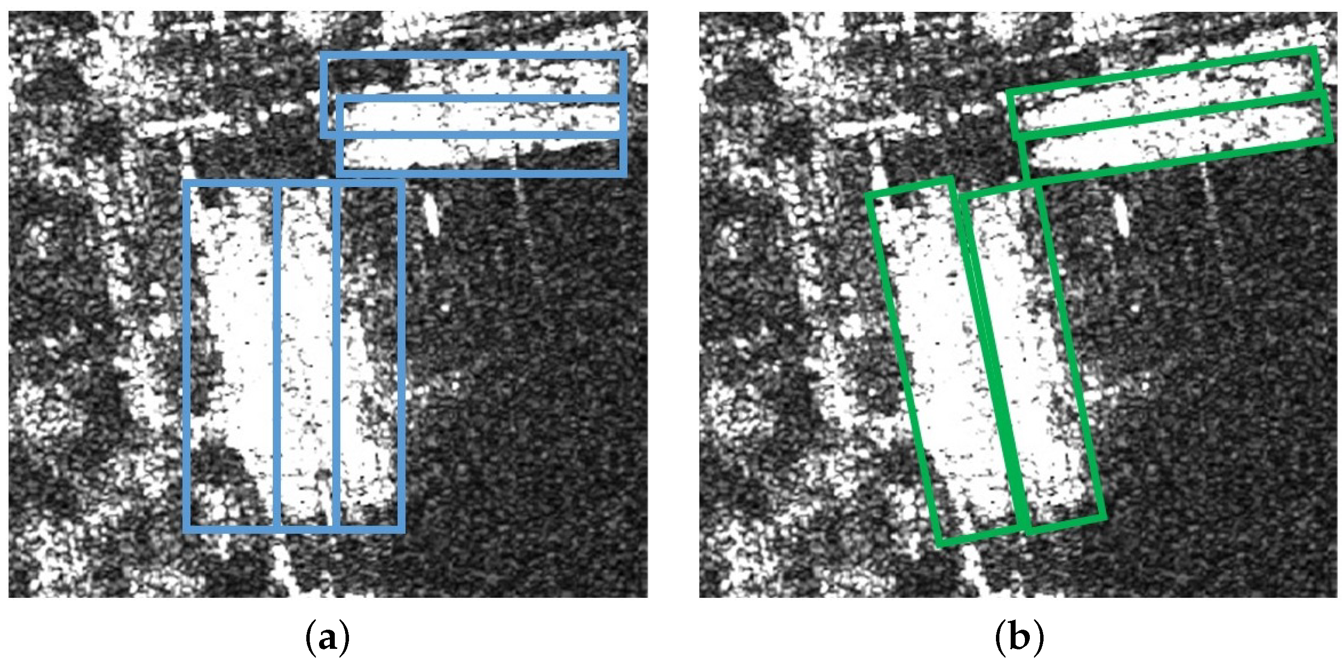
2. Arbitrary-Oriented Ship Detection in SAR Images

In this section, the commonly used RBB encodings and their problems are first introduced, then the long-edge decomposition RBB encoding is demonstrated in detail. Secondly, for the problem of the positive and negative sample imbalance in the SAR ship images, the multiscale elliptical Gaussian sample balancing strategy is introduced. Finally, the model structure and details of the algorithm are presented.

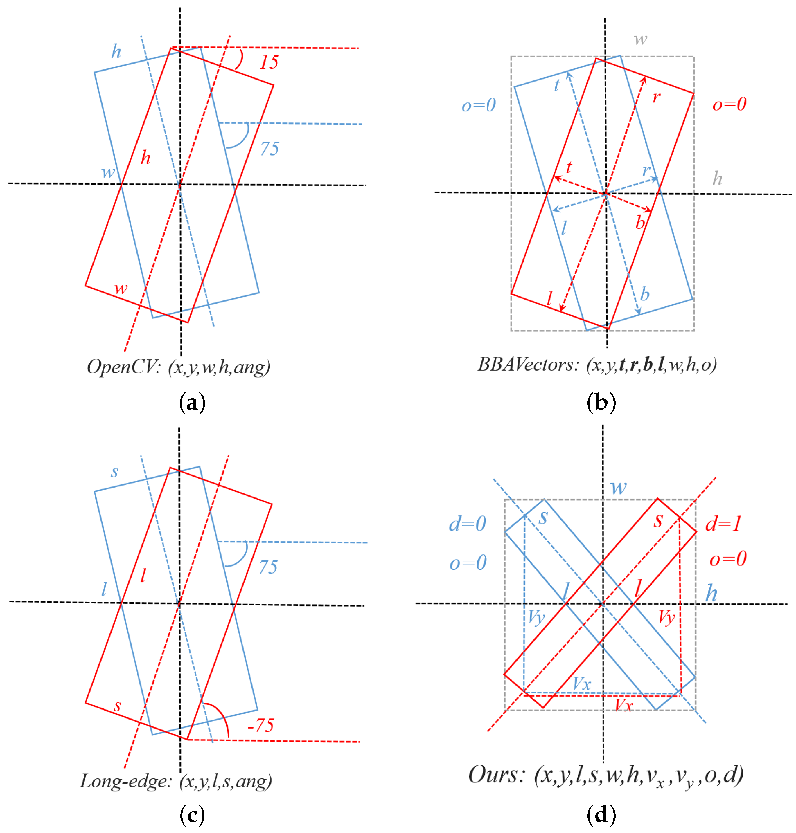
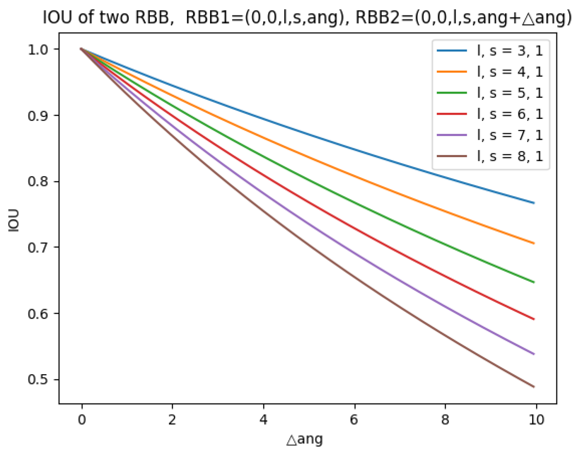
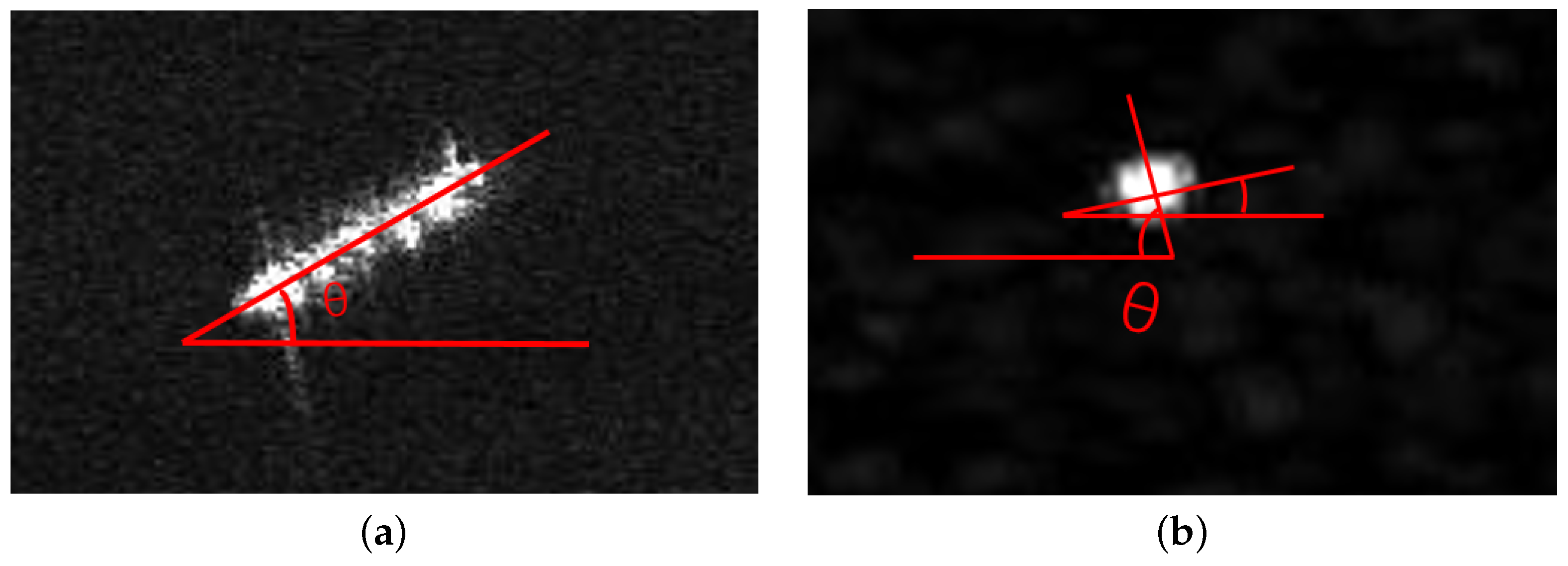
2.1. Classic RBB Encodings

The RBB encoding is mainly divided into two categories, according to whether it is angle-based or not. For example, OpenCV encoding and long-edge encoding are both the angle-based encodings, which are the two most commonly used RBB encodings. Another class encoding does not characterize the orientation of the rotated box via the angle, such as BBAVectors encoding. It takes the offset vectors of four edges from the center point to represent the RBB. Figure 2a–c give the schematic diagram of the three RBB encodings. In the two sides of the boundary states, the wide and high edge of the OpenCV-encoded RBB have been interchanged, and their angle difference is large due to the periodicity of the angle. During the training, the EOE problem makes it difficult for the model to distinguish the wide and high edges of the neighboring vertical and horizontal targets, which may result in an inaccurate predicted height and width of such targets. Due to the POA problem, even though the prediction box basically matches the ground truth, the loss between them is still large for the large angle difference, which makes it difficult for the loss function to guide the learning of the model. The long-edge RBB encoding avoids the EOE problem but still suffers from the POA problem. The BBAVectors encoding also suffers from the EOE problem, which makes it difficult for the model to distinguish the neighboring vectors when in the boundary case [24].

The relationship curves of the IOU and angle deviation between two RBBs encoded by the angle-based RBB encoding with different aspect ratios is presented in Figure 3. It can be found that the larger the aspect ratio, the higher the impact of the angle deviation on the IOU, which tends to cause a poor IOU score for the large aspect ratio targets [25]. Therefore, to deal with these problems, the long-edge decomposition RBB encoding is proposed as follows.

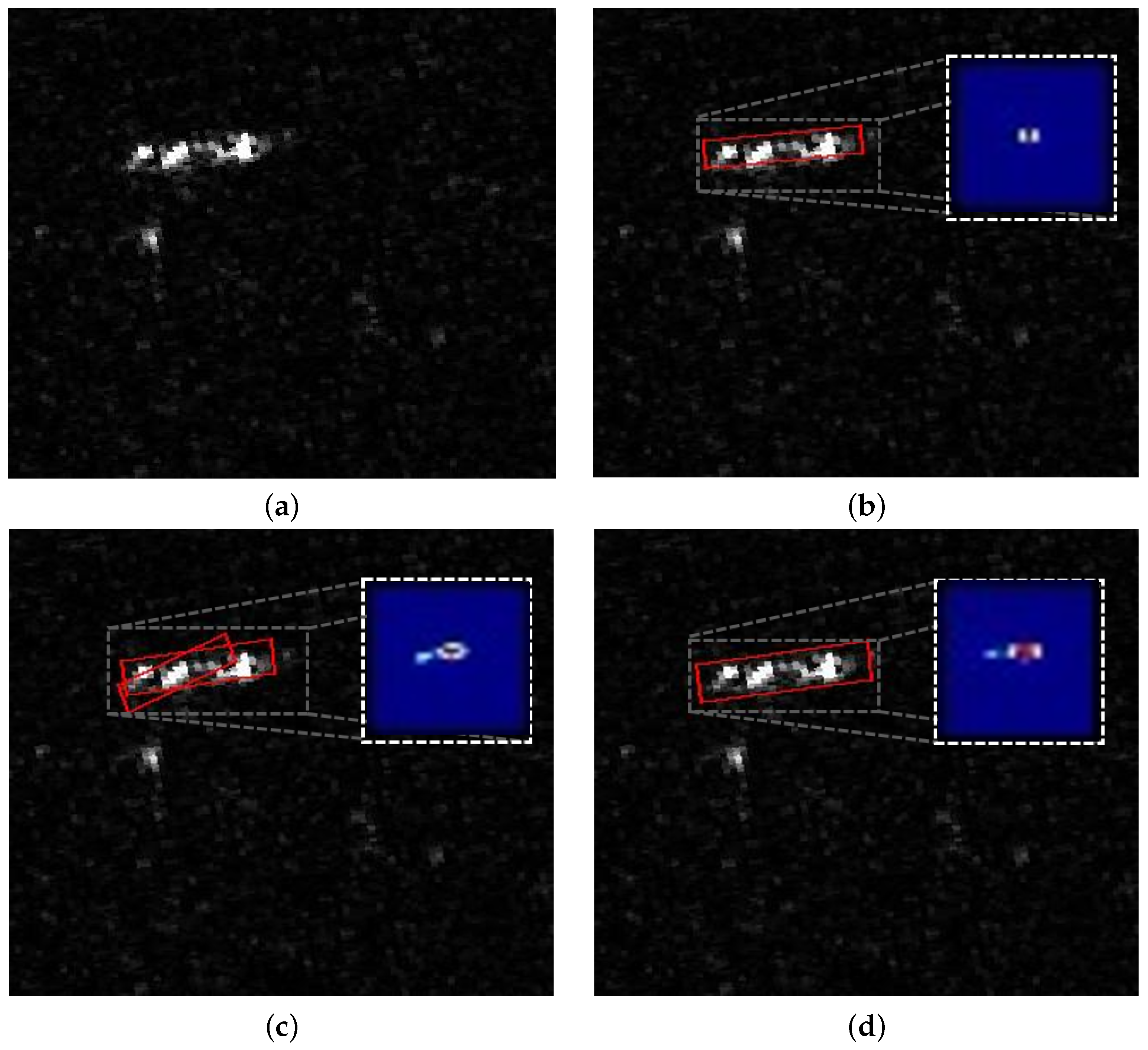
2.2. Long-Edge Decomposition RBB Encoding

The long-edge decomposition encoding takes advantage of the fact that the long-edge features of the ships in SAR images are more representative of their orientation. This encoding does not directly describe the orientation of the ships via the angle, but takes the length of the horizontal and vertical components of the long edge of the ship targets, as shown in Figure 2d. In Figure 2d, x and y denote the center point of the target, and l and s denote the length of the long and short edges of the target, respectively. $v_x$ and $v_y$ denote the components of the long edge in the horizontal and vertical axis directions, o is the box type selection field. $v_x$ and $v_y$ are not normalized to enlarge the weight of the large-size targets in the loss function, which makes the model pay more attention to the large-size targets with significant directional information and facilitates the regression of the orientation information of the ship targets. The arc tangent of the ratio of the $v_x$ and $v_y$ is calculated to represent the angle of the rotated box, but results in ambiguity in its tilt direction. Therefore, we clarify this ambiguity by disguising which side of the vertical axis the upper end of the target is located in. When d equals to 1, it means the upper end of the rotated box faces the right, while when d equals 0, it means that it is facing the left. It is found that the code words of our proposed encoding are consistent on both sides of the boundary state, except that the tilt direction d takes the opposite value. So, our proposed encoding avoids the boundary discontinuity problem in a simple and effective way.

In the boundary case, the ship target can be approximately horizontal or vertical. To prevent the model from making mistakes in the determination of the ship tilt direction, the HBB is directly adopted to locate such ship targets. Furthermore, since the orientation information of the square-like ship targets is not obvious, as shown in Figure 4, it is hard for the model to predict the accurate orientation of such ship targets. Although the angle error of the square-like ship targets has a smaller attenuation on the IOU, it is better to use the HBB directly to locate them.

Thus, the model also regresses the width and height of the external horizontal box along with the parameters of the rotated one. Moreover, the IOU between the rotated box and its external horizontal box is taken as the criteria to determine which kind of box should be selected to locate the corresponding targets, in the same way as the method mentioned in [24]. The IOU is higher for the ship targets that are neighboring horizontal or vertical and for the square-like ship targets than the others. Thus, the method of obtaining the code word for our proposed long-edge decomposition RBB encoding from the coordinates of the four corner points is presented in Algorithm 1.

The model directly regresses each parameter of long-edge decomposition RBB encoding during the training, and then decodes it to locate the ship target in the inference stage. In the decoding stage, the horizontal box will be selected to locate the target, if the prediction value of the box-type selection field is above the threshold or the angle is around 90 and 0 degrees, otherwise the rotated box would be selected. As the decoding detail illustrates in Algorithm 2, based on the information provided in the encodings, it is not hard to obain the four corner points of the RBB or HBB which specify the target location.

Algorithm 1 Encoding.

Input:$Pi$, i = 1,2,3,4, the bottom, left, top, and right corner points of RBB Output:(x, y , l, s, w, h, $v_x$, $v_y$, o, d), code words of long-edge decomposition encoding 1: calculate the width and height of the HBB 2: w = $max$($Pi\left[0\right]$, i = 1,2,3,4)-$min$($Pi\left[0\right]$, i = 1,2,3,4) 3: h = $max$($Pi\left[1\right]$, i = 1,2,3,4)-$min$($Pi\left[1\right]$, i = 1,2,3,4) 4: calculate the long side and short side of the RBB 5: $Le1$ = $|P3-P2|$, $Le2$ = $|P3-P4|$; l = $max$($Le1,Le2$), s = $min$($Le1$, $Le2$) 6: calculate long-edge decompositions and tilt direction 7: if$Le1>Le2$then 8:  ($v_x$, $v_y$) = $\left|\right(P3+P4)-(P1+P2\left)\right|$ 9:    $d=1$ 10: else 11:    ($v_x$, $v_y$) = $\left|\right(P3+P2)-(P1+P4\left)\right|$ 12:    $d=0$ 13: end if 14: calculate target center 15: (x, y) = $sum(Pi,i=1,2,3,4)/4$ 16: decide the box type 17: if IOU (HBB, RBB)>0.9 then 18:    $o=1$ 19: else 20:    $o=0$ 21: end if 22: return ($x,y,l,s,w,h,$$v_x$, $v_y$, $o,d$)

Algorithm 2 Decoding.

Input: ($x,y,l,s,w,h$, $v_x$, $v_y$, $o,d$), code words Output: $Pi$, i = 1,2,3,4, coordinates of the bottom, left, top, and right corner points 1: calculate four corner points of HBB 2: ( $P1,P2,P3,P4$) = ($(x-w/2,y+h/2),(x-w/2,y-h/2),(x+w/2,y-h/2),(x+w/2,y+h/2)$) 3: calculate angle 4: if$v_y$ > = $v_x$ then 5:    $Theta$ = $atan$($v_y$/ $v_x$) 6: else 7:    $Theta$ = 90-$atan$($v_x$ / $v_y$) 8: end if 9: if ($Theta$ > 89 or < 1) or o >0.5 then 10:    return ( $P1,P2,P3,P4$) 11: end if 12: calculate the offset between the four RBB corner points and center 13: $l_x$, $l_y$, $s_x$, $s_y$ = $l/2*cos\left(Theta\right),l/2*sin\left(Theta\right),s/2*sin\left(Theta\right),s/2*cos\left(Theta\right)$ 14: calculate four corner points of RBB 15: if$d>0.5$then 16:    $P1,P2,P3,P4$ = ( x-$l_x$+$s_x$, y+$l_y$+$s_y$), (x-$l_x$-$s_x$, y+$l_y$-$s_y$), (x+$l_x$-$s_x$, y-$l_y$-$s_y$), (x+$l_x$+$s_x$, y-$l_y$+$s_y$) 17: else 18:    $P1,P2,P3,P4$ = ( x+$l_x$-$s_x$, y+$l_y$+$s_y$), (x-$l_x$-$s_x$, y-$l_y$+$s_y$), (x-$l_x$+$s_x$, y-$l_y$-$s_y$), (x+$l_x$+$s_x$, y+$l_y$-$s_y$) 19: end if 20: return ( $P1,P2,P3,P4$)

Figure 5 shows the relationship curves between the prediction deviation of $v_x$, $v_y$ and the IOU between two RBBs which are neighboring boundary state. Because the $v_x$ is small for the targets neighboring vertical, its relative prediction error may be larger. Luckily, thanks to the large $v_y$, this error does not result in accountable errors on the angle calculated from the arc tangent between $v_x$ and $v_y$, which is used for the calculation of the corner points of the RBB as illustrated in Algorithm 2. As a result, the IOU between the two RBBs remains relatively high. In the general case, if the model converges well, the relative errors in the prediction long-edge decomposition are small due to their large true values.

At the same time, the horizontal and vertical long-edge components are not normalized in this paper, and the same prediction error has less influence on the angle calculation value of the target with the larger size, so it is not easy to have the problem that the IOU of the target with the large aspect ratio is not high. Based on the shape characteristics of the ships, the long-edge decomposition RBB encoding is applicable to the detection of the oriented ship targets, which can avoid the POA problem and EOE problem and facilitate the convergence of the model. In addition, the whole encoding and decoding processes of our proposed RBB encoding method are very simple but effective.

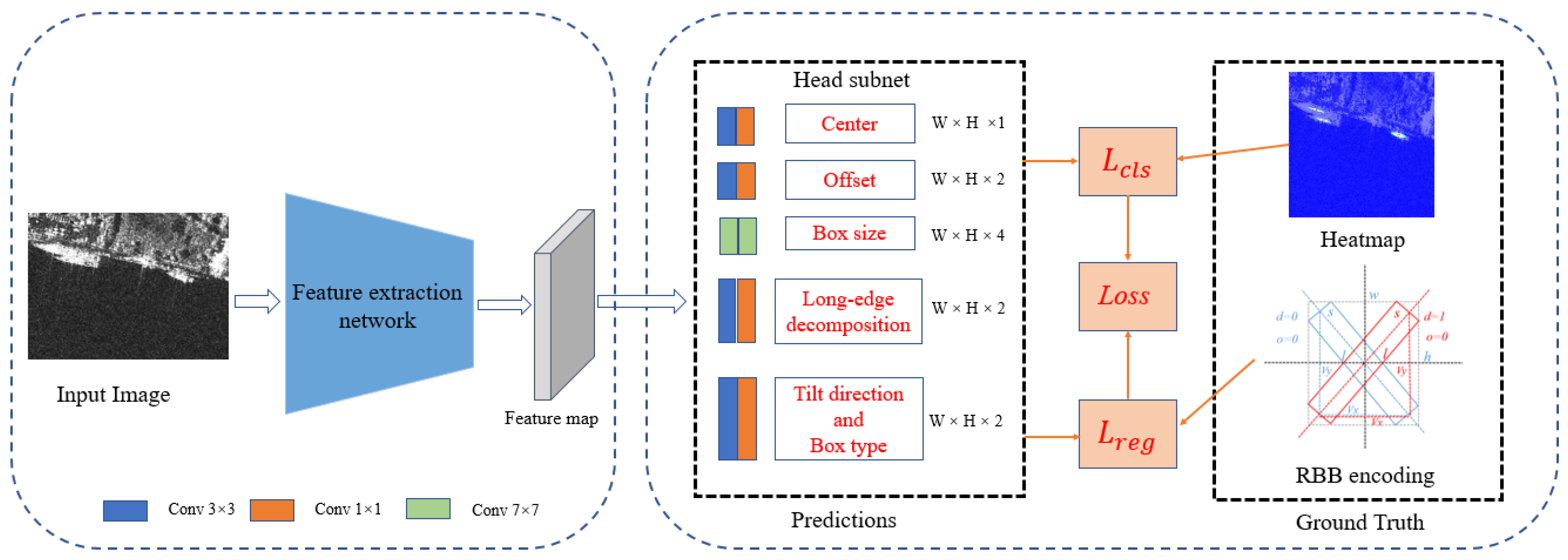
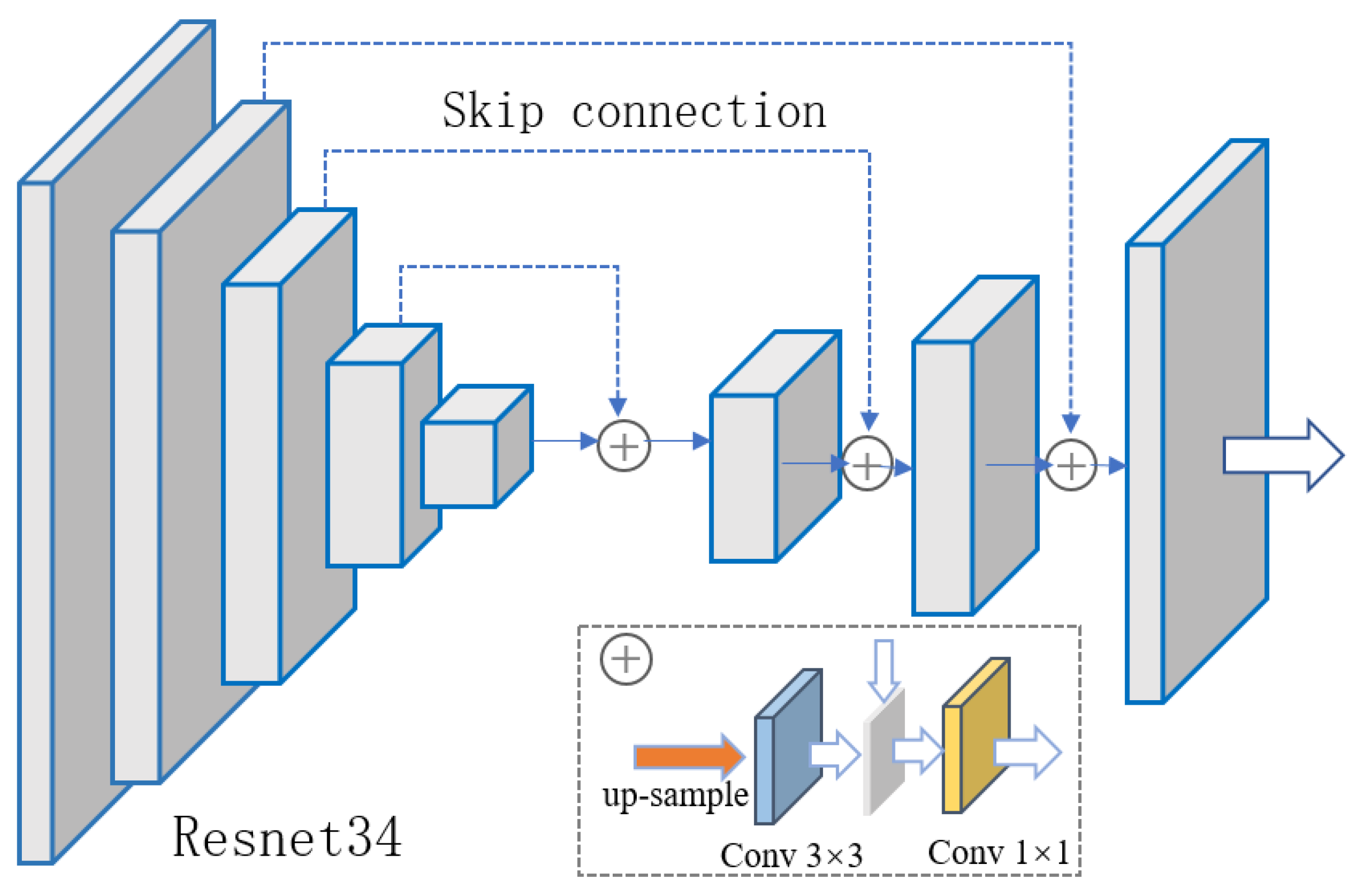
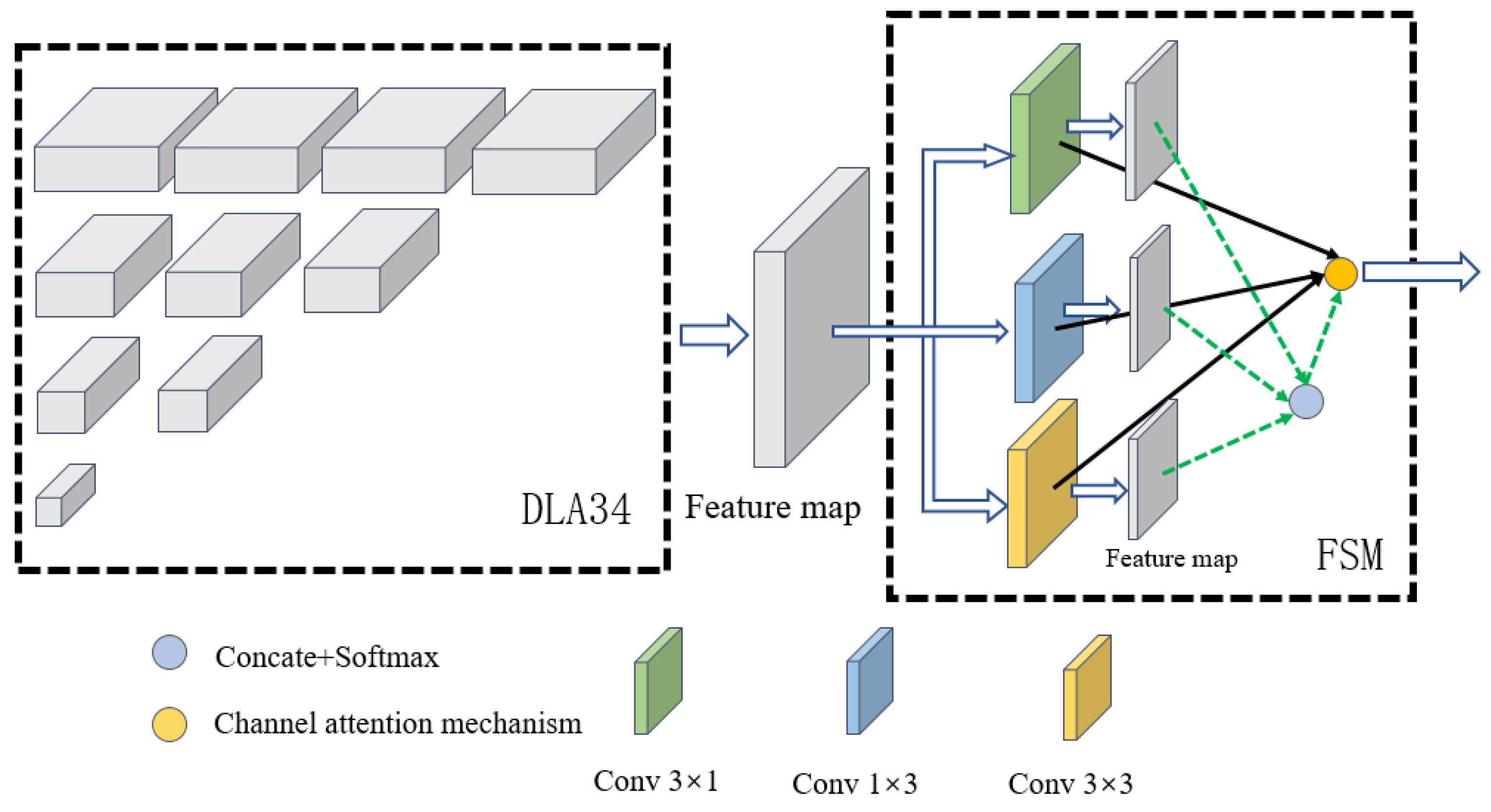
2.3. Model Structure

Anchors of various sizes and angles are required for the anchor-based methods to regress the location of the oriented ship targets. To achieve high precision, a large number of preset anchors are required, which may lead to a waste of computational resources due to the imbalance of positive and negative samples. So, the anchor-free method is more suitable for the task of ship detection in SAR images when computational resources are limited. Therefore, the anchor-free detector CenterNet is taken as the base model for the subsequent experiments, the structure of the model is shown in Figure 6. The model is composed of a backbone network and a head network. The backbone network is used to extract the features of the ship targets in the image, while the head network regresses the location and size parameters of the ship targets.

The ship targets span a wide size range in SAR images, thus both the high-level semantic information and low-level detail information should be retained for detecting the ship targets of different sizes. Thus, the well-established feature extraction network shown in Figure 7 is used for the subsequent experiments, where the ResNet34 [29] can extract the deep semantic information while preventing the shallow detail information from being lost through the skip connections. Then, a feature pyramid is selected to further fuse the features from the different layers to facilitate the subsequent detection task for the targets of different sizes. The head subnet is responsible for the regression of the parameters of the long-edge decomposition RBB encoding, and each branch consists of two convolutional layers. Among them, the center prediction module outputs a heatmap representing the distribution of the target center location. In the forward stage, the positions with an amplitude greater than the 8 points around them are selected as the candidate target center points through max pooling with a 3 × 3 kernel. Among these, candidate target center points, whose amplitude exceeds the confidence threshold, are selected as the final predicting target centers. The offset prediction module is used to correct the errors that arose from the stage of calculating the ground truth of the target center distribution heatmap. The box size module is responsible for the regression of the length of the long and short edges of the rotated box and the size of the horizontal box. Then, the long-edge decomposition module is responsible for regressing the projection of the ship long edge on the horizontal and vertical directions, which is used to characterize the ship orientation information. The tilt direction and box type prediction module is used to identify whether the top end of the ship is located in the left or right of the vertical axis and to decide whether the HBB or the RBB shall be selected to position the corresponding targets.

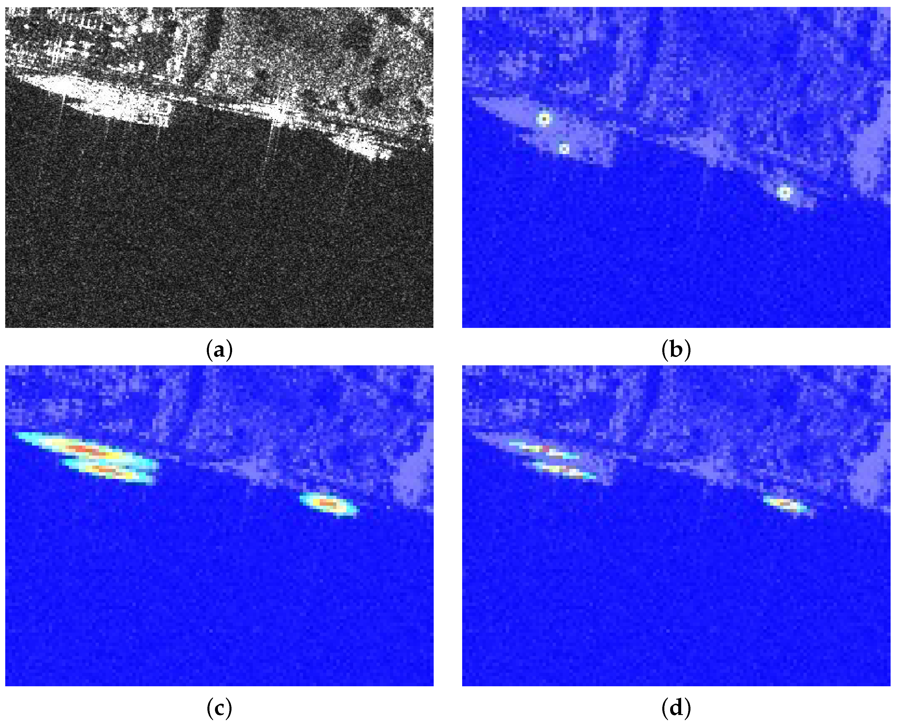
2.4. Multiscale Elliptical Gaussian Sample Balancing Strategy

Each pixel in the heatmap output from the center prediction module of the model is a sample, which corresponds to the location in the original image and is associated with the features of the corresponding area [30]. Consistent with the CenterNet, the center point of each target on the heatmap is taken as the positive sample, having a pixel value of one, while the rest are considered as the negative samples, having a pixel value of less than one. The closer to the center of the target, the greater the pixel value of the negative sample points. Furthermore, a higher value of a point on the heatmap indicates a higher probability of a target at that location. The Focal loss [20] is generally used to train the sample points in the anchor-free detectors for the single-category target detection task, which is given by

$$\begin{array}{c}\begin{array}{cc}\hfill L_{cls}& =L_{focal-loss}(Y_{xy},\stackrel{\wedge }{Y_{xy}})\hfill \\ \hfill & =\frac{1}{N}{\sum }_{xy}\left\{\begin{array}{cc}{(1-\stackrel{\wedge }{Y_{xy}})}^{\alpha }log\left(\stackrel{\wedge }{Y_{xy}}\right)& Y_{xy}=1\\ {(1-Y_{xy})}^{\beta }{\left(\stackrel{\wedge }{Y_{xy}}\right)}^{\alpha }log(1-\stackrel{\wedge }{Y_{xy}})& otherwise\end{array}\right.\hfill \end{array}\end{array}$$

(1)

where $Y_{xy}$ denotes the ground truth of the heatmap, and $\stackrel{\wedge }{Y_{xy}}$ denotes the prediction value of the heatmap. The Focal loss function uses two groups of the factors, including the positive and negative sample weights and difficult and simple sample weights, to adjust the model attention to different samples.

Figure 8b is an example of the heatmap of the CenterNet [12], which uses the circular Gaussian kernel to label the weights of the sample points nearly around the target center. It is obvious that the weights of the most negative samples are equal to one, which is same as that of the positive samples, thus the loss of the negative sample dominates because the number of the negative samples is much higher than that of the positive samples. For the inshore areas, such as the ports with the large area of the complex terrestrial background interference, the problem is more serious because of the large number of the hard-negative samples, which may cause the target to be missed. Thus, we label the loss weight of the negative samples within the foreground target region via an elliptical Gaussian distribution, which is given in (2). Combining (1) and (2), it is easy to see that the closer the negative samples are to the target center, the smaller the loss weight. That is to say, the closer the features are to the target center region, the more desirable they are to be retained.

$$\begin{array}{c}\begin{array}{c}\begin{array}{cc}\hfill Y_{xy}& =f(x,y)\hfill \\ \hfill & =\left\{\begin{array}{cc}exp\left[\frac{-1}{2}{\left[\begin{array}{c}x-c_x\\ y-c_y\end{array}\right]}^T{C}^{-1}\left[\begin{array}{c}x-c_x\\ y-c_y\end{array}\right]\right]& ,(x,y)\in foreground\\ 0& ,otherwise\end{array}\right.\hfill \end{array}\end{array}\end{array}$$

(2)

where x and y denote a point on the heatmap, $c_x$ and $c_y$ denote the target center coordinates, C is the covariance matrix whose specific expression is given by (3) and (4).

$$\begin{array}{c}\begin{array}{c}\begin{array}{c}\begin{array}{cc}\hfill C& =R\mathsf{\Lambda }{R}^T\hfill \\ \hfill & =\left[\begin{array}{cc}cos\theta & -sin\theta \\ sin\theta & cos\theta \end{array}\right]\left[\begin{array}{cc}{L_1}^2& 0\\ 0& {L_2}^2\end{array}\right]\left[\begin{array}{cc}cos\theta & sin\theta \\ -sin\theta & cos\theta \end{array}\right]\hfill \\ \hfill & =\left[\begin{array}{cc}{v}_x/l& -v_y/l\\ v_y/l& v_x/l\end{array}\right]\left[\begin{array}{cc}{f}_1{\left(l\right)}^2& 0\\ 0& {(0.7\ast f_1\left(s\right))}^2\end{array}\right]\left[\begin{array}{cc}{v}_x/l& v_y/l\\ -v_y/l& v_x/l\end{array}\right]\hfill \end{array}\end{array}\end{array}\end{array}$$

(3)

$$\begin{array}{c}\begin{array}{cc}\hfill f_1\left(x\right)& =\left\{\begin{array}{cc}\lambda \ast x\ast min(\sqrt{\frac{s_{min}}{size}},\frac{3}{2})& size<s_{min}\\ \lambda \ast x\ast \sqrt{\frac{{\mathrm{s}}_{max}}{size}}& size>={\mathrm{s}}_{max}\\ \lambda \ast x& size\in else\end{array}\right.\hfill \end{array}\end{array}$$

(4)

In (3), the rotation matrix R determines the orientation of the elliptical Gaussian kernel, the elements ${L_1}^2$ and ${L_2}^2$ in the diagonal matrix $\mathsf{\Lambda }$ determine the length of the long edge and short edge of the elliptical Gaussian kernel. To make the elliptical Gaussian kernel more slender, adjustment factor 0.7 is set in (3). This is to prevent feature overlapping between adjacent ships when ship targets are lined up close together. l and s denote the lengths of the long and short edges of the ship, $v_x$ and $v_y$ denote the long-edge components in the horizontal and vertical direction, respectively. Furthermore, the $s_{min}$ and $s_{max}$ in (4) denote the size threshold, $size$ denotes the target area, $\lambda$ equals 0.2 in the experiments. The 3/2 in Equation (4) is a hyper parameter which sets the upper limit of the length and width of the elliptical Gaussian kernel corresponding to the small target.

The interference that the imbalance of the positive and negative samples pose on the ship targets with different sizes are different. The features of large-size targets are naturally more likely to be retained. Even if the loss of the negative samples dominates, their features are still not easily suppressed. The retained features of the small targets after the feature extraction stage are weaker, which would be easily suppressed due to the excessive loss of the negative sample, resulting in the missed detection. For this reason, the function $f_1$ in (4) is taken to adjust the area of the elliptical Gaussian kernel corresponding to the targets of different sizes. The area of the elliptical Gaussian kernel corresponding to the large targets is restricted, while the area of the elliptical Gaussian kernel corresponding to the small targets is improved. We found that the elliptical Gaussian kernel is also used in recent research [31] to label the loss weights of the negative sample within the target region, but they do not adjust the area according to the target size. An instance of its heatmap is shown in Figure 8c, the elliptical Gaussian kernel covers the entire ship target area, which would preserve the large area of the features of the large size targets, thus it may cause the problem of repeated detection. An example of the heatmap of our proposed method is shown in Figure 8d, the elliptical Gaussian kernel covers the small ship, while the area of the elliptical Gaussian kernel corresponding to the large target is restricted. It alleviates the missed detection of the small targets due to the sample imbalance, and it is also less likely to lead to the repeated detection of large targets.

2.5. Loss Function

Corresponding to the tasks of each branch of the head subnet, the training loss consists of three parts. The center prediction module classifies each sample point on the heatmap and is trained via the focal loss, which is shown in (1)–(4). The smooth L1 function is selected to train the box size prediction module, the offset correction module, and the long-edge decomposition module, because they all belong to the regression problem, which is shown in (5)–(7).

$$\begin{array}{c}\begin{array}{c}\hfill L_S=L_{Smooth-L1}(S,\stackrel{\wedge }{S})\end{array}\end{array}$$

(5)

$$\begin{array}{c}\begin{array}{c}\hfill L_{off}=L_{Smooth-L1}(f,\stackrel{\wedge }{f})\end{array}\end{array}$$

(6)

$$\begin{array}{c}\begin{array}{c}\hfill L_{v_x{v}_y}=1.5(1-e^{1-\frac{l}{s}})L_{Smooth-L1}(V,\stackrel{\wedge }{V})\end{array}\end{array}$$

(7)

where S denotes the target size, f denotes the center point offset, V denotes the long-edge decomposition. l and s denote the long and short edges of the target, respectively, and $\mathsf{\Lambda }$ denotes the prediction value of that variable. For the long-edge decomposition module, because the orientation information of the circular-like ships in SAR images is ambiguous, the loss of such targets shall not be taken into account during training to avoid their interference with the model convergence process. The orientation characteristics of the targets of the large aspect ratio are more significant, which is conducive to the regression of the orientation information of the target, thus the loss weight of such target needs to be enhanced. So, we take aspect ratio as the weighting factor to adjust the loss weight of each target, the higher the aspect ratio, the larger the loss weight, and the long-edge decomposition module pays more attention to such ship targets. Function $1.5(1-e^{1-\frac{l}{s}})$ is used to smooth the loss weights of each target with different aspect ratios. The weight equals 0 when the aspect ratio equals 1, and the upper limit of loss weight is set to 1.5 in the experiments, as shown in (7).

Both the box type selection module and tilt direction module are trained via the binary cross-entropy loss, since the tasks they deal with belong to the binary classification problems, which can be given by (8)–(10).

$$\begin{array}{c}\begin{array}{c}\hfill L_{bce-loss}(Y,\stackrel{\wedge }{Y})=\frac{1}{N}\sum _{n=1}^N-[y_{n}log\stackrel{\wedge }{y_n}+(1-y_n).log(1-\stackrel{\wedge }{y_n})]\end{array}\end{array}$$

(8)

$$\begin{array}{c}\begin{array}{c}\hfill L_r=L_{bce-loss}(r,\stackrel{\wedge }{r})\end{array}\end{array}$$

(9)

$$\begin{array}{c}\begin{array}{c}\hfill L_d=L_{bce-loss}(d,\stackrel{\wedge }{d})\end{array}\end{array}$$

(10)

where $r=\{0,1\}$ is the box type selection parameter, $d=\{0,1\}$ is the tilt direction parameter. The total training loss can be given by the following:

$$\begin{array}{c}\begin{array}{c}\hfill L={\lambda }_{cls}{L}_{cls}+{\lambda }_{off}{L}_{off}+{\lambda }_s{L}_s+{\lambda }_{v_x{v}_y}{L}_{v_x{v}_y}+{\lambda }_r{L}_r+{\lambda }_d{L}_d\end{array}\end{array}$$

(11)

where the weights in (11) are hyper parameters, which are set to 1, 1, 0.5, 1, 1, and 1, respectively, in the following experiments.

3. Experiments and Discussion

3.1. Experimental Settings and Evaluation Metrics

The computer used for the experiments is configured with the basic hardware, such as the Intel i7-9700K 8G CPU and NVIDIA RTX 2060s Ti 8G GPU. The experiments were developed based on the Ubuntu 18.04 operating system and Pytorch 1.7.1 software framework, and then the model training process was accelerated via the cuda 10.2. The SSDD [13] dataset was used in these experiments, which is a benchmark for the oriented ship target detection in the SAR image, with a total of 1160 SAR ship images containing the ship targets of various sizes and angles, as well as the images of different scenes, such as the inshore port areas and offshore sea areas. The SAR images in the SSDD dataset are mainly acquired by RadarSat-2, TerraSAR-X, and Sentinel-1 radars with four types of polarization (HH, HV, VV, and VH), as well as the different resolutions. The average size of the images in the dataset is 481 × 331. In this experiment, the training and test sets are divided in a ratio of 4:1, without setting a validation set to make full use of the image data. In the experiments, the Adam optimizer was used to update the model parameters, and then the initial learning rate and batch size were set to 0.000125 and 8, respectively. Exponential decay strategy with a decay factor of 0.95 was used to adjust the learning rate. In each experiment, the model was trained for enough epochs, and the optimal one among these model parameters saved for each epoch during the training was selected.

In this paper, the precision rate $Pd$, recall rate $Rd$, $F_1$ score, average precision $Ap$, and repeated detection rate $R{D}_1$ and $R{D}_2$ are used to evaluate the experimental results, which are calculated as follows:

$$Pd=\frac{T_p}{T_p+F_p}$$

(12)

$$Rd=\frac{T_p}{T_p+F_n}$$

(13)

$$F_1=\frac{2\ast Pd\ast Rd}{Pd+Rd}$$

(14)

$$Ap=\underset{0}{\overset{1}{\int }}p\left(r\right)dr$$

(15)

$$R{D}_1=\frac{T_p+F_p}{T_p}$$

(16)

$$R{D}_2=\frac{T_p+F_p}{T_p+F_n}$$

(17)

where $T_p$ denotes the number of correct detection boxes, $F_p$ denotes the number of false detection boxes, $F_n$ denotes the number of undetected targets. $p\left(r\right)$ denotes the relationship curve between the precision rate and recall rate. $Pd$ indicates the ratio of correctly detected targets among all prediction boxes, $Rd$ calculates the ratio of the detected targets to the number of all targets, $F_1$ and $Ap$ are taken to evaluate the performance of models in the comprehensive perspective. If not specifically stated in this paper, the IOU threshold is set to 0.5. That is say, the target is considered to be successfully detected if the IOU between the prediction box and ground truth exceeds 0.5.

3.2. Comparison Experiments of Different Encodings

To verify the effectiveness of the long-edge decomposition encoding, the comparison experiments between our proposed encoding and classic RBB encodings used for the ship target detection in the SAR image have been presented. The network shown in Figure 6 and the feature extraction network shown in Figure 7 constitute the experimental model. The head network is different in order to regress the different encodings. These modules in the head subnet consist of one 3 × 3 convolution layer cascaded with one 1 × 1 convolution layer, except for the box size module which consists of two 7 × 7 convolution layers.

The experimental results of the different RBB encodings are shown in

Table 1. Experimental Results of the Different RBB Encodings.

RBB Encodings	$\mathit{Pd}$	$\mathit{Rd}$	$\mathit{Ap}$	${\mathit{F}}_1$
Opencv encoding	0.938	0.901	0.886	0.919
Long-edge encoding	0.953	0.915	0.898	0.933
BBAVectors encoding	0.952	0.933	0.902	0.942
Ours encoding	0.952	0.939	0.908	0.945

. From the metrics of the $Rd$, $Ap$, and $F_1$ score, our proposed encoding can achieve the optimal results, which are 0.939, 0.908, and 0.945, respectively. Furthermore, our proposed encoding also scored the second in the $Pd$, which is 0.952. On the other hand, the BBAVectors encoding achieves the second highest scores in the $Pd$, $Rd$, $Ap$, and $F_1$ scores, which are 0.952, 0.933, 0.902, and 0.942, respectively. The long-edge encoding scored the highest in the $Pd$, while it scored the third in $Rd$, $Ap$, and $F_1$.

The $Ap$ and $F_1$ scores achieved by the model based on the different RBB encodings at the higher IOU thresholds are given in Figure 9. The model based on the long-edge decomposition RBB encoding achieves the highest $Ap$ and $F_1$ scores. The $Ap$ and $F_1$ scores of the OpenCV RBB-encoding-based model and long-edge RBB-encoding-based model do not differ much in the experimental results. The $Ap$ and $F_1$ scores of the BBAVectors-encoding-based model decreased significantly as the IOU threshold increases. The results reflect that the model regressing our encoding is better at framing the oriented ship targets.

Figure 10 represents the detection results of the model based on the four RBB encodings for the ship target neighboring boundary states. As shown in Figure 10b, for the ships neighboring vertical, the angle and size prediction errors of the OpenCV RBB-encoding-based model are large. In the top row of Figure 10c, the detection box of the long-edge RBB-encoding-based model does not match the vertical ship in the bottom-right of the picture, due to its relatively large angle error, and there are cases of missing detection. As shown in Figure 10d, rotated bounding boxes are selected by the BBAVectors RBB-encoding-based model to locates ships which are neighboring boundary state, but they do not match these ships well enough. The ship target detection results of the long-edge decomposition RBB-encoding-based model is shown in Figure 10e, the oriented ships and the ships neighboring boundary state can be accurately located via the rotated boxes and horizontal boxes, respectively.

According to the experimental results, the model using the OpenCV method may be affected by EOE and POA problems, and it is difficult to distinguish the wide edge and high edge of the vertical and horizontal targets, so the problem of the large width and height prediction errors of the vertical angle targets arises. The long-edge encoding suffers from the POA problem, which interferes in the convergence of the model, which may result in the large angle prediction error for ships neighboring boundary state. The BBAVectors uses the horizontal boxes to locate the horizontal or vertical angle targets. If the box type is selected incorrectly, due to EOE problems, the detection RBB of the ships close to horizontal or vertical may not match the ship targets accurately, as shown in Figure 10d. Furthermore, the long tail at the right end of the ship caused by strong scattering points, shown in the bottom row of Figure 10d, also interferes with the prediction of the top, right, and bottom vectors of the BBAVectors encoding, which may be another contribution to the poorly matched detection box.

Furthermore, the coding lengths of OpenCV RBB encoding, long-edge RBB encoding, BBAVectors RBB encoding, and long-edge decomposition RBB encoding are 5, 5, 13, and 10, respectively. The number of model parameters based on these encoding methods are 24.28 M, 24.28 M, 24.38 M, and 24.45 M, and the corresponding inference time costs of a single image based on the experimental device are 15.55 ms, 15.55 ms, 15.7 ms, and 16.13 ms, respectively, which shows little difference. Therefore, the effectiveness of long-edge decomposition RBB encoding can be proved based on the above analysis.

3.3. Experiments of the Multiscale Elliptical Gaussian Sample Balancing

In this section, we compare the performances of these three methods introduced in Section 2.4, which includes the circular Gaussian sample balancing strategy (CGSBS), the elliptical Gaussian sample balancing strategy (EGSBS), and our proposed multiscale elliptical Gaussian sample balancing strategy (MEGSBS).

A comparison result of these sample balancing strategies is given in Figure 11, where the pixel values of the target area in the heatmap output from the models based on the EGSBS and our proposed MEGSBS are stronger. However, the heatmap output from the model based on the EGSBS [31] shows two strong separated peak points, which leads to the repeated detection of the single ship target and, thus, postprocessing, such as the NMS, is needed to remove the repeated detection boxes.

Table 2. Experimental Results of the Different Sample Balancing Strategies.

Strategies	$\mathit{Pd}$	$\mathit{Rd}$	$\mathit{Ap}$	${\mathit{F}}_1$
CGSBS (with NMS or not)	0.952	0.939	0.908	0.945
EGSBS (w/o NMS)	0.848	0.961	0.872	0.901
EGSBS (w NMS)	0.917	0.961	0.916	0.938
MEGSBS (w/o NMS)	0.948	0.964	0.923	0.956
MEGSBS (w NMS)	0.955	0.964	0.930	0.960

gives the experimental results of the different sample balancing strategies. It can be found that the EGSBS and MEGSBS outperform the CGSBS in terms of the $Rd$. That proves the capability of these two methods to reduce the probability of the missing detection due to the dominating negative sample. However, the precision of the EGSBS-based model is lower. In particular, the $Pd$ is only 0.848 without NMS post-processing. After the NMS, its $Pd$ increases by 0.069, while the $Pd$ of the model based on the MEGSBS only increases by 0.007 after NMS post-processing. Furthermore, when ships locate closely together, due to the difficulty of detection, the inaccurate prediction boxes of adjacent ship targets would be removed by NMS processing, which is also one contribution of the increment in $Pd$ after NMS processing. So, it is not difficult to find that the MEGSBS is less likely to result in repeated detection.

As a rule of the thumb, missed detection is a common issue in small-target detection tasks, while repeated detection is more prevalent in large-target detection tasks. Thus, to further analyze these problems, the recall rates for small targets (top 30 pc of targets with smallest size) and the repeated detection rates for large targets (top 30 pc of targets with largest size) of the model based on different sample balancing strategies are given in

Table 3. Recall Rate for Small Ships and Repeated Detection Rate for Large Ships.

Metrics	Circular Gaussian	Elliptical Gaussian	Multiscale Elliptical Gaussian
Rd (Top 30 pc)	0.914	0.928	0.934
$R{D}_1$ (Bttm 30 pc)	1.014	1.418	1.034
$R{D}_2$ (Bttm 30 pc)	0.941	1.362	1.013

. The definitions of the repeated detection rate ($R{D}_1$ and $R{D}_2$) in Table 3 are given in (16) and (17), respectively. According to the data in Table 3, it can be found that the MEGSBS-based model has a higher recall rate for small targets compared to the other two, and also has a lower repeated detection rate for large targets. The EGSBS-based model, on the other hand, shows a big increase in the repeated detection rate, although there is some improvement in the recall rate for small targets. Therefore, combining the data in Table 2 and Table 3, we can conclude that MEGSBS can effectively alleviate the problem of missed detection for small targets caused by the positive and negative sample imbalance problem, and also is less likely to lead to the repeated detection of large targets.

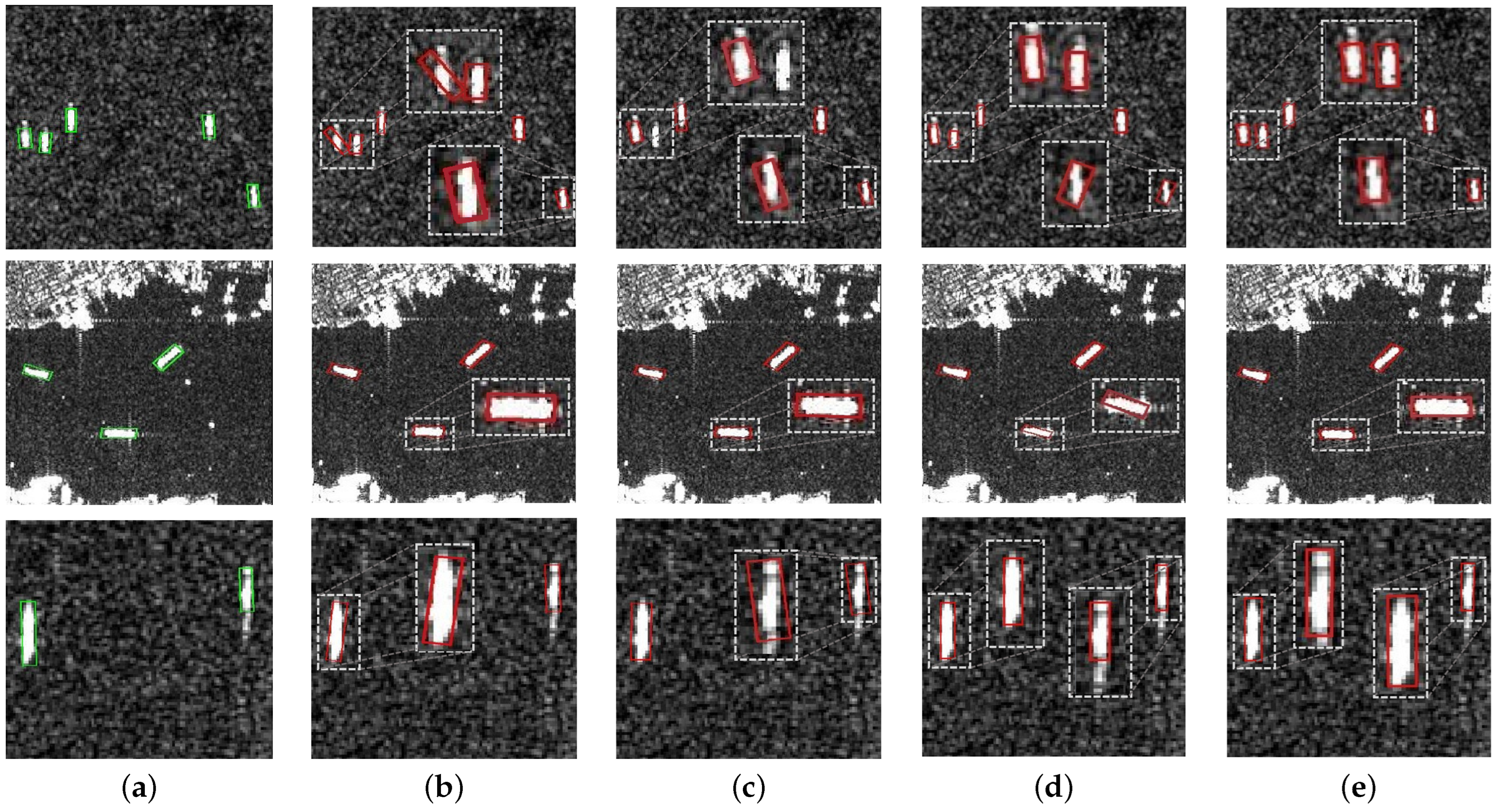
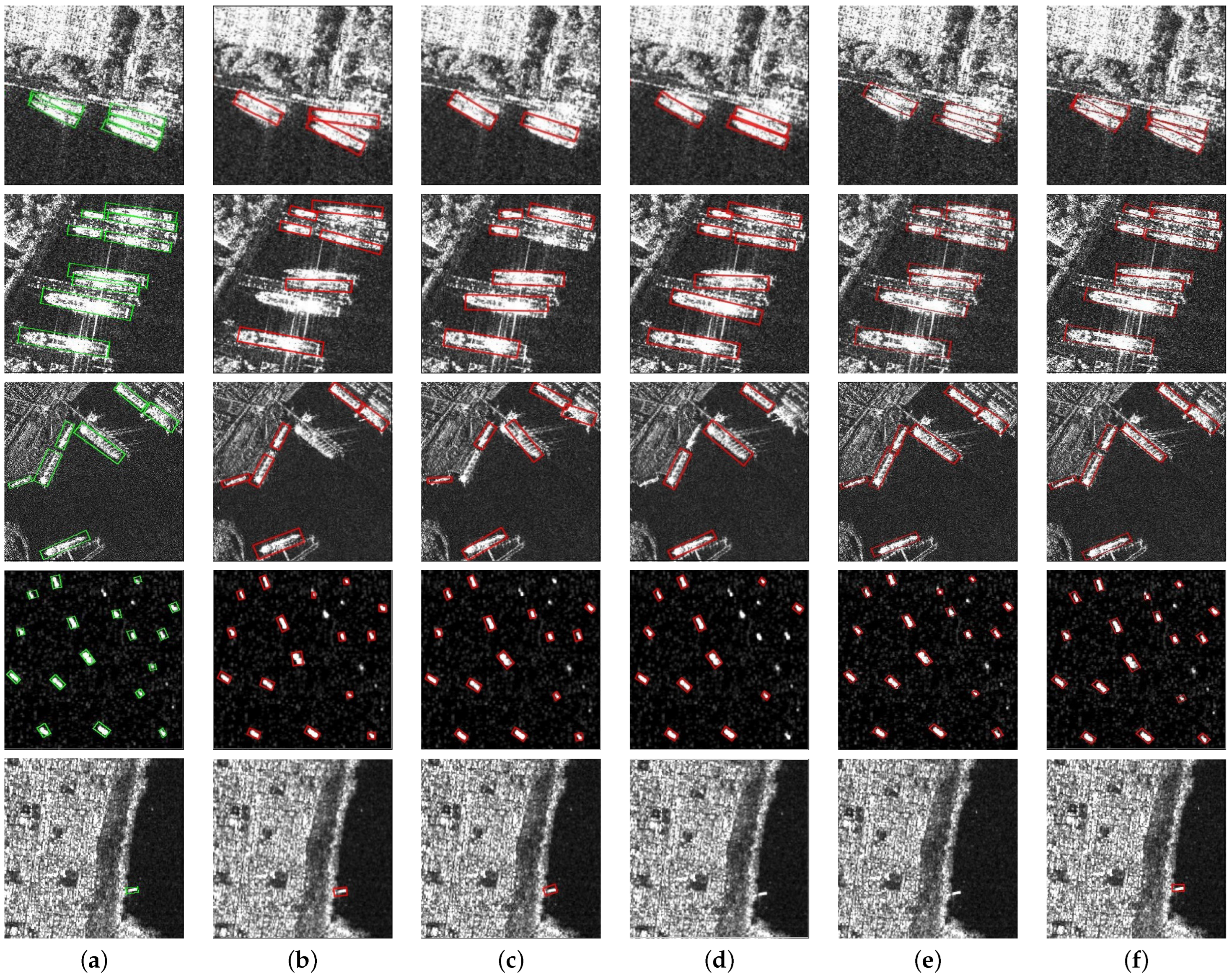
3.4. Comparison Experiments with the Mainstream Detection Methods

To verify the overall effectiveness of our proposed method, the existing mainstream detection methods of the oriented ships are selected for comparison experiments in this section, which mainly includes the ROItransformer [32], Rotated-Retinanet, Rotated-Fcos, and BBAVectors [24]. The ROItransformer belongs to the two-stage anchor-based model, which extracts the rotated rectangular region of interest (ROI) for the subsequent training that helps the model to extract features for the oriented targets. Rotated-Retinanet is the expansion of the Retinanet from the HBB-based target detection to the RBB-based target detection, which is a single-stage anchor-based detector that locates the targets directly by optimizing the difference between the target and the anchor without extracting the ROI. The Rotated-FCOS expanded from the FCOS is an anchor-free detector that uses the feature maps of the different depths, which can detect the ship targets of the different sizes and use the centerness [10] to remove the poorly matched boxes. The BBAVectors detector proposed in [24] also belongs to the anchor-free detector, which regresses the vectors between the four edges and the center point to represent the RBB for target locating.

In order to further validate the transferability of our proposed method, we also conducted another experiment based on the model shown in Figure 6 which applied another feature extraction network shown in Figure 12. As shown in Figure 12, the DLA34 [33] has been adopted as the backbone network for feature extraction, which deeply aggregates the features at the different levels through the tree structure and finally outputs the feature map with the downsampling rate of four. The feature selection network (FSM) [34] has been used as the neck network to sample the features extracted from the backbone network via the convolutional operators, with the different receptive fields. It consists of three convolution layers with the kernel sizes of 3 × 3, 1 × 3, and 3 × 1, which can extract the feature of the different orientations and increase the differentiation between these neighboring targets. Moreover, the feature maps of each branch are weighted and fused via the channel attention mechanism, which are then input to the head subnet in a subsequent process.

Table 4. Experimental Results of Different Detection Methods.

Detection Methods	Parameters Quantity (M)	$\mathit{Pd}$	$\mathit{Rd}$	$\mathit{Ap}$	${\mathit{F}}_1$
Rotated-Retinanet	36.35	0.825	0.868	0.832	0.846
ROItransformer	55.25	0.905	0.921	0.913	0.913
Rotated-FCOS	51.11	0.891	0.925	0.911	0.908
BBAVectors	24.38	0.952	0.933	0.902	0.942
Ours (Dla34 + FSM)	20.72	0.949	0.955	0.925	0.952
Ours (Res34 + FPN)	24.45	0.948	0.964	0.923	0.956

gives the detailed experimental results of the different detection methods. It can be seen that our proposed method achieves the highest scores in the $Rd$, $Ap$, and $F1$ score, which are 0.964, 0.925, and 0.956, respectively, and the $Pd$ reached the second score of 0.949. The BBAVectors detector achieved the highest score of 0.952 in the $Pd$. Meanwhile, the number of the parameters of our proposed model is the smallest among these models, only 20.72M. In addition, the performances of the Rotated-FCOS and ROItransformer are similar, with the average precision of about 0.91 and the model parameter quantity of about 50M. It should be noted that the MEGSBS is applied in our proposed method in the experiments of this section.

Figure 13 gives the detection results of the different detection methods for the inshore large ship targets (in first three rows ), offshore small ship targets (in the fourth row) and inshore small ship targets (in the fifth row). Figure 13f show that our proposed model can accurately locate the large target and small target in the complex inshore area and simple offshore area. Figure 13d–e shows that both Rotated-FCOS and BBAVectors have the problem of the missing detection of ship targets under the complex background interference, as well as the missing detection of small targets. Figure 13c shows that the ROItansformer suffers from these problems of inaccurate positioning and missing detection of adjacent ship targets. It may be caused by the inability to generate the rotated ROI which accurately extracts the whole ship in the case that the ships are lined up together, thus in turn aggravating the feature overlapping. In Figure 13b, the Rotated-Retinanet also suffers from the inaccurate localization and missed detection of the ship targets in the complex inshore area, which may be caused by the inability of the anchors of limited sizes and angles to match the various sizes and angles of the ship targets.

4. Conclusions

The proposed long-edge decomposition RBB encoding takes advantage of the fact that the long-edge features of the ship targets in SAR images are more representative of their orientation, and it avoids the boundary discontinuity problem caused by the EOE and POA, which is helpful to the convergence of the models. In order to avoid the influence that comes from the ambiguous orientation of the ship targets with small aspect ratios, and to avoid the inaccurate location that may result from the wrong decision on the tilt direction of the ship targets in the boundary state, our proposed model regresses a horizontal box as a supplement to locate these two types of ship targets. The results of the ablation experiments have showed that the proposed long-edge decomposition RBB encoding is effective for the oriented ship detection in the SAR images. Meanwhile, the SAR ship images suffer from the imbalance of the positive and negative samples, and the ship targets of different sizes are subject to varying degrees of interference caused by this problem. Therefore, the multiscale elliptical Gaussian kernel has been proposed to adjust the loss weight of the negative samples within the target foreground area. It can reduce the loss weight of the negative samples for the small- and medium-sized targets, which can alleviate the missing detection problem due to the over high negative sample loss. Compared with the elliptical Gaussian kernel without the size adjustment, it is also less likely to lead to the repeated detection of large targets due to the excessive attenuation of the loss weight of the negative samples. Finally, the experimental results verify the correctness and effectiveness of our proposed long-edge decomposition RBB encoding and the multiscale elliptical Gaussian sample balancing strategy. In the follow-up research, we will continue to try to experiment on more models (such as the ReDet [35], Oriented R-CNN [36], and YOLO series) and datasets. Furthermore, we will also try to apply the proposed RBB encoding and sample balancing strategy to other model structures in the future.

References

1. Xie, H.; An, D.; Huang, X.; Zhou, Z. Efficient raw signal generation based on equivalent scatterer and subaperture processing for one-stationary bistatic SAR including motion errors. IEEE Trans. Geosci. Remote Sens. 2016, 54, 3360–3377. [Google Scholar] [CrossRef]
2. Xie, H.; Shi, S.; An, D.; Wang, G.; Wang, G.; Xiao, H.; Huang, X.; Zhou, Z.; Xie, C.; Wang, F.; et al. Fast factorized backprojection algorithm for one-stationary bistatic spotlight circular SAR image formation. IEEE J. Sel. Top. Appl. Earth Obs. Remote Sens. 2017, 10, 1494–1510. [Google Scholar] [CrossRef]
3. Xie, H.; Hu, J.; Duan, K.; Wang, G. High-efficiency and high-precision reconstruction strategy for P-band ultra-wideband bistatic synthetic aperture radar raw data including motion errors. IEEE Access 2020, 8, 31143–31158. [Google Scholar] [CrossRef]
4. An, D.; Wang, W.; Zhou, Z. Refocusing of ground moving target in circular synthetic aperture radar. IEEE Sens. J. 2019, 19, 8668–8674. [Google Scholar] [CrossRef]
5. Li, J.; An, D.; Wang, W.; Zhou, Z.; Chen, M. A novel method for single-channel CSAR ground moving target imaging. IEEE Sens. J. 2019, 19, 8642–8649. [Google Scholar] [CrossRef]
6. Lang, H.; Xi, Y.; Zhang, X. Ship detection in high-resolution SAR images by clustering spatially enhanced pixel descriptor. IEEE Trans. Geosci. Remote Sens. 2019, 57, 5407–5423. [Google Scholar] [CrossRef]
7. Gao, G.; Liu, L.; Zhao, L.; Shi, G.; Kuang, G. An adaptive and fast CFAR algorithm based on automatic censoring for target detection in high-resolution SAR images. IEEE Trans. Geosci. Remote Sens. 2008, 47, 1685–1697. [Google Scholar] [CrossRef]
8. Ren, S.; He, K.; Girshick, R.; Sun, J. Faster r-cnn: Towards real-time object detection with region proposal networks. IEEE Trans. Pattern Anal. Mach. Intell. 2017, 39, 1137–1149. [Google Scholar] [CrossRef] [PubMed] [Green Version]
9. Redmon, J.; Divvala, S.; Girshick, R.; Farhadi, A. You only look once: Unified, real-time object detection. In Proceedings of the IEEE Conference on Computer Vision and Pattern Recognition, Las Vegas, NV, USA, 27–30 June 2016; pp. 779–788. [Google Scholar]
10. Tian, Z.; Shen, C.; Chen, H.; He, T. Fcos: Fully convolutional one-stage object detection. In Proceedings of the IEEE/CVF International Conference on Computer Vision (ICCV), Seoul, Republic of Korea, 27 October–2 November 2019; pp. 9627–9636. [Google Scholar]
11. Law, H.; Deng, J. CornerNet: Detecting objects as paired keypoints. Int. J. Comput. Vis. 2020, 128, 642–656. [Google Scholar] [CrossRef] [Green Version]
12. Zhou, X.; Wang, D.; Krähenbühl, P. Objects as points. arXiv 2019, arXiv:1904.07850. [Google Scholar]
13. Li, J.; Qu, C.; Shao, J. Ship detection in SAR images based on an improved faster R-CNN. In Proceedings of the 2017 SAR in Big Data Era: Models, Methods and Applications (BIGSARDATA), Beijing, China, 13–14 November 2017; pp. 1–6. [Google Scholar]
14. Xiaoling, Z.; Tianwen, Z.; Jun, S.; Shunjun, W. High-speed and high-accurate SAR ship detection based on a depthwise separable convolution neural network. J. Radars 2019, 8, 841–851. [Google Scholar]
15. Redmon, J.; Farhadi, A. Yolov3: An incremental improvement. arXiv 2018, arXiv:1804.02767. [Google Scholar]
16. Fu, J.; Sun, X.; Wang, Z.; Fu, K. An anchor-free method based on feature balancing and refinement network for multiscale ship detection in SAR images. IEEE Trans. Geosci. Remote Sens. 2020, 59, 1331–1344. [Google Scholar] [CrossRef]
17. Guo, H.; Yang, X.; Wang, N.; Gao, X. A CenterNet++ model for ship detection in SAR images. Pattern Recognit. 2021, 112, 107787. [Google Scholar] [CrossRef]
18. An, Q.; Pan, Z.; Liu, L.; You, H. DRBox-v2: An improved detector with rotatable boxes for target detection in SAR images. IEEE Trans. Geosci. Remote Sens. 2019, 57, 8333–8349. [Google Scholar] [CrossRef]
19. Liu, W.; Anguelov, D.; Erhan, D.; Szegedy, C.; Reed, S.; Fu, C.Y.; Berg, A.C. Ssd: Single shot multibox detector. In Proceedings of the European Conference on Computer Vision, Amsterdam, The Netherlands, 11–14 October 2016; pp. 21–37. [Google Scholar]
20. Lin, T.Y.; Goyal, P.; Girshick, R.; He, K.; Dollár, P. Focal loss for dense object detection. In Proceedings of the IEEE International Conference on Computer Vision (ICCV), Venice, Italy, 22–29 October 2017; pp. 2980–2988. [Google Scholar]
21. Yang, R.; Pan, Z.; Jia, X.; Zhang, L.; Deng, Y. A novel CNN-based detector for ship detection based on rotatable bounding box in SAR images. IEEE J. Sel. Top. Appl. Earth Obs. Remote Sens. 2021, 14, 1938–1958. [Google Scholar] [CrossRef]
22. Yang, X.; Hou, L.; Zhou, Y.; Wang, W.; Yan, J. Dense label encoding for boundary discontinuity free rotation detection. In Proceedings of the IEEE/CVF Conference on Computer Vision and Pattern Recognition, Nashville, TN, USA, 19–25 June 2021; pp. 15819–15829. [Google Scholar]
23. Yang, X.; Yan, J. Arbitrary-oriented object detection with circular smooth label. In Proceedings of the European Conference on Computer Vision (ECCV), Glasgow, UK, 23–28 August 2020; pp. 677–694. [Google Scholar]
24. Yi, J.; Wu, P.; Liu, B.; Huang, Q.; Qu, H.; Metaxas, D. Oriented object detection in aerial images with box boundary-aware vectors. In Proceedings of the IEEE/CVF Winter Conference on Applications of Computer Vision, Waikoloa, HI, USA, 3–8 January 2021; pp. 2150–2159. [Google Scholar]
25. He, Y.; Gao, F.; Wang, J.; Hussain, A.; Yang, E.; Zhou, H. Learning polar encodings for arbitrary-oriented ship detection in SAR images. IEEE J. Sel. Top. Appl. Earth Obs. Remote Sens. 2021, 14, 3846–3859. [Google Scholar] [CrossRef]
26. Yang, X.; Yan, J.; Ming, Q.; Wang, W.; Zhang, X.; Tian, Q. Rethinking rotated object detection with gaussian wasserstein distance loss. arXiv 2022, arXiv:2101.11952. [Google Scholar]
27. Yang, X.; Yang, X.; Yang, J.; Ming, Q.; Wang, W.; Tian, Q.; Yan, J. Learning high-precision bounding box for rotated object detection via kullback-leibler divergence. Adv. Neural Inf. Process. Syst. 2021, 34, 18381–18394. [Google Scholar]
28. Shrivastava, A.; Gupta, A.; Girshick, R. Training region-based object detectors with online hard example mining. In Proceedings of the IEEE Conference on Computer Vision and Pattern recognition (CVPR), Las Vegas, NV, USA, 27–30 June 2016; pp. 761–769. [Google Scholar]
29. He, K.; Zhang, X.; Ren, S.; Sun, J. Deep residual learning for image recognition. In Proceedings of the IEEE Conference on Computer Vision and Pattern Recognition (CVPR), Las Vegas, NV, USA, 27–30 June 2016; pp. 770–778. [Google Scholar]
30. Zhu, C.; Chen, F.; Shen, Z.; Savvides, M. Soft anchor-point object detection. In Proceedings of the European Conference on Computer Vision (ECCV), Glasgow, UK, 23–28 August 2020; pp. 91–107. [Google Scholar]
31. Shiqi, C.; Wei, W.; Ronghui, Z.; Jun, Z.; Shengqi, L. A lightweight, arbitrary-oriented SAR ship detector via feature map-based knowledge distillation. J. Radars 2022, 11, 1–14. [Google Scholar]
32. Ding, J.; Xue, N.; Long, Y.; Xia, G.S.; Lu, Q. Learning RoI transformer for oriented object detection in aerial images. In Proceedings of the IEEE Conference on Computer Vision and Pattern Recognition (CVPR), Long Beach, CA, USA, 15–20 June 2019; pp. 2849–2858. [Google Scholar]
33. Yu, F.; Wang, D.; Shelhamer, E.; Darrell, T. Deep layer aggregation. In Proceedings of the IEEE Conference on Computer Vision and Pattern Recognition (CVPR), Salt Lake City, UT, USA, 18–23 June 2018; pp. 2403–2412. [Google Scholar]
34. Pan, X.; Ren, Y.; Sheng, K.; Dong, W.; Yuan, H.; Guo, X.; Ma, C.; Xu, C. Dynamic refinement network for oriented and densely packed object detection. In Proceedings of the IEEE Conference on Computer Vision and Pattern Recognition (CVPR), Seattle, WA, USA, 13–19 June 2020; pp. 11207–11216. [Google Scholar]
35. Han, J.; Ding, J.; Xue, N.; Xia, G.S. Redet: A rotation-equivariant detector for aerial object detection. In Proceedings of the IEEE/CVF Conference on Computer Vision and Pattern Recognition (CVPR), Nashville, TN, USA, 20–25 June 2021; pp. 2786–2795. [Google Scholar]
36. Xie, X.; Cheng, G.; Wang, J.; Yao, X.; Han, J. Oriented R-CNN for object detection. In Proceedings of the IEEE/CVF International Conference on Computer Vision (ICCV), Montreal, BC, Canada, 11–17 October 2021; pp. 3520–3529. [Google Scholar]
Figure 1. Comparison of the different bounding boxes for locating the oriented ship targets. (a) HBB; (b) RBB.
Remotesensing 15 00673 g001
Figure 2. Schematic diagram of the different RBB encodings: (a) Opencv encoding; (b) long-edge encoding; (c) BBAVectors encoding; (d) our proposed encoding.
Remotesensing 15 00673 g002
Figure 3. Relationship curves of the IOU and angle deviation for the angle-based encodings.
Remotesensing 15 00673 g003
Figure 4. Two SAR ship instances with different shapes. (a) Ship with a big aspect ratio presents an obvious orientation; (b) square-like ship presents an obscure orientation.
Remotesensing 15 00673 g004
Figure 5. Relationship curves between the prediction deviation of v x , v y and the IOU: (a) IOU vs. prediction error of v x ; (b) IOU vs. prediction error of v y .
Remotesensing 15 00673 g005
Figure 6. Model structure.
Remotesensing 15 00673 g006
Figure 7. Feature extraction network (Res34 + FPN).
Remotesensing 15 00673 g007
Figure 8. Heatmap instance: (a) SAR ship image; (b) circular Gaussian kernel; (c) elliptical Gaussian kernel; (d) multiscale elliptical Gaussian kernel.
Remotesensing 15 00673 g008
Figure 9. Histogram of the A p and F 1 score under the different IOU thresholds.
Remotesensing 15 00673 g009
Figure 10. Detection results of the models based on the different encodings for the ships under the boundary cases: (a) ground truth; (b) OpenCV encoding; (c) long-edge encoding; (d) BBAVectors encoding; (e) our proposed encoding.
Remotesensing 15 00673 g010
Figure 11. The detection results of the model based on different sample balancing strategies and corresponding heatmaps: (a) original picture; (b) circular Gaussian; (c) elliptical Gaussian; (d) multiscale elliptical Gaussian.
Remotesensing 15 00673 g011
Figure 12. Feature extraction network (Dla34 + FSM).
Remotesensing 15 00673 g012
Figure 13. Detection results of the different detection methods: (a) ground truth; (b) Rotated-Retinanet; (c) ROItransformer; (d) Rotated-FCOS; (e) BBAVectors; (f) our proposed method (Dla34+FSM). First three rows: inshore large ship targets in the SAR image. Fourth row: offshore small ship targets in the SAR image. Fifth row: inshore small ship targets in the SAR image.
Remotesensing 15 00673 g013