
A Texture Feature Removal Network for Sonar Image Classification and Detection


College of Intelligent Systems Science and Engineering, Harbin Engineering University, Harbin 150009, China
*
Author to whom correspondence should be addressed.
Remote Sens. 2023, 15(3), 616; https://doi.org/10.3390/rs15030616
Submission received: 21 November 2022
/
Revised: 8 January 2023
/
Accepted: 17 January 2023
/
Published: 20 January 2023
(This article belongs to the Special Issue Advancement in Undersea Remote Sensing)
Abstract
:Deep neural network (DNN) was applied in sonar image target recognition tasks, but it is very difficult to obtain enough sonar images that contain a target; as a result, the direct use of a small amount of data to train a DNN will cause overfitting and other problems. Transfer learning is the most effective way to address such scenarios. However, there is a large domain gap between optical images and sonar images, and common transfer learning methods may not be able to effectively handle it. In this paper, we propose a transfer learning method for sonar image classification and object detection called the texture feature removal network. We regard the texture features of an image as domain-specific features, and we narrow the domain gap by discarding the domain-specific features, and hence, make it easier to complete knowledge transfer. Our method can be easily embedded into other transfer learning methods, which makes it easier to apply to different application scenarios. Experimental results show that our method is effective in side-scan sonar image classification tasks and forward-looking sonar image detection tasks. For side-scan sonar image classification tasks, the classification accuracy of our method is enhanced by 4.5% in a supervised learning experiment, and for forward-looking sonar detection tasks, the average precision (AP) is also significantly improved.
1. Introduction
Autonomous detection and recognition of underwater targets were always the focuses of research. Side-scan sonar and forward looking sonar sensors became the most widely used sensors in underwater detection because they have long detection distances, are not affected by water quality, and can provide high-definition two-dimensional images [1,2,3,4]. Traditional sonar image target detection and recognition methods are mostly based on manual feature extraction combined with classifier [5,6]. These methods are sensitive to parameter settings, and when the underwater sediment changes and sonar sensors change, their applicability deteriorates [1].
In recent years, deep learning technology made great achievements in the field of image recognition, and in many aspects, the recognition ability of deep learning exceeded that of human beings. However, at present, deep learning technology is still based on the support of large labeled datasets and achieves high classification and recognition ability after long-term training.
The acquisition of sonar images requires considerable manpower and material resources, and for a water area, it is unknown whether the underwater environment contains targets; that is, when scanning the water area, it is unknown whether the obtained sonar images contain targets, which further leads to the scarcity of sonar image samples containing specific targets. Due to the scarcity of samples, training a deep neural network from scratch on such a small dataset is challenging, which may cause severe overfitting, making it difficult to realize universal applicability to sonar target recognition tasks.
The same problem is also encountered in medical image recognition, remote sensing image recognition, and many other fields. Among many solutions, transfer learning is a very effective method [7]. For example, in [8,9,10,11,12,13,14], researchers used transfer learning methods for medical image classification or detection tasks, and in [15], Lumini et al. adopted a transfer learning method to identify underwater organisms. New material discoveries were even been made based on transfer learning methods. An approach using transfer learning with feature extraction for building an identification system of mildew disease in pearl millet was proposed by [16], and Chen et al. [17] used a convolutional neural network and transfer learning method to identify and diagnose plant diseases automatically, which is highly important in the field of agricultural information.
In practice, a person who learned to play tennis can learn badminton faster than others since both tennis and badminton share some common knowledge, which is the basic key to transfer learning. Inspired by human capabilities to transfer knowledge across domains, transfer learning aims to leverage knowledge from a related domain (called the source domain) to improve the learning performance or minimize the number of labeled examples required in a target domain [7]. Transfer learning is widely used in areas that lack data. Many papers [18,19] reported the use of transfer learning technology to identify COVID-19.
Pires de Lima et al. [19] systematically reviewed transfer learning applications for scene classification using various datasets and deep-learning models, and the results show that transfer learning provides a powerful tool for remote-sensing scene classification. Different from common transfer learning methods, You et al. [20] studied the task adaptive pretrained model selection-based transfer learning method, which selects the best models from a model zoo without fine-tuning, and the logarithm of maximum evidence (LogME) was proposed, in which a pretrained model with a high LogME value is likely to have good transfer performance. You et al. [21] found that in transfer learning, task-specific layers are usually not fully fine-tuned; hence, they are unable to maximize the transfer of knowledge. They proposed a two-step framework named ”cotuning”. Cotuning collaboratively supervises the fine-tuning process by providing a detailed relationship analysis of samples and labels between the source domain and target domain. The experimental results show that cotuning can result in a relative improvement of up to 20%. Guo et al. [22] proposed an adaptive fine-tuning approach called ”SpotTune”. The key strategy of SpotTune is finding the optimal fine-tuning strategy per instance for the target data. Given an image that corresponds to the target task, a policy network is used to make routing decisions on whether to pass the image through the fine-tuned layers or the pretrained layers. SpotsTune outperformed the traditional fine-tuning approach on 12 out of 14 standard datasets. Shafahi et al. [23] improved the LwF loss to make it suitable for use in transfer learning. The loss function was designed to make the feature representations of the source and target network similar, thereby preserving the robust feature representations.
Transfer learning methods are also widely used in sonar image target detection and recognition tasks. For example, for submarine pipeline maintenance, Chen et al. [24] used forward-looking sonar to detect submarine pipelines, and inspired by saliency segmentation, they developed a forward-looking sonar image segmentation method and improved the efficiency of AUVs. Yulin et al. [25] proposed an improved Faster-RCNN model for detecting wreckage targets in side-scan sonar images. They improved the object classification part of Faster-RCNN by equalizing the number of anchor boxes in the region proposal network that either contain or do not contain wreckage targets and employing a balanced sampling of the image database for model training. Experiments show that the improvement leads to 4.3% higher detection accuracy on the dataset they built. Zhou et al. [26] studied a lightweight neural network in sonar image classification tasks and found that the lightweight CNN achieves better results at a smaller cost, which renders it more suitable for actual engineering applications. Yu et al. [27] integrated a transformer module and YOLOv5, and an attention mechanism was also introduced into the method to meet the requirements of accuracy and efficiency for underwater target recognition. The experimental results show that their method achieves better results in terms of both accuracy and time consumption. Chandrashekar et al. [28] studied the classification of several objects, such as sand, mud, clay, graves, ridges, and sediments, in the underwater sea using side-scan sonar images. They utilized a deep learning-based transfer learning approach, and experiments showed that after fine-tuning the parameters in object recognition, the accuracy was greatly improved. Huo et al. [1] used a transfer learning method to transfer the knowledge from the ImageNet dataset to a side-scan sonar image dataset that they built, and during transfer, they proposed a semisynthetic data generation method for producing sonar images, which can greatly compensate for insufficient data. Ochal et al. [29] evaluated and compared several supervised and semisupervised few-shot learning (FSL) methods using underwater optical and side-scan sonar imagery, and the results show that FSL methods offer significant advantages over simple transfer learning methods, such as fine-tuning a pretrained model.
In transfer learning methods, the differences between source and target domains are called domain gaps, and the fundamental purpose of transfer learning is to narrow them. Many transfer learning methods were proposed and achieved very good results, such as DANN [30], JAN [31], and TLDA [32]. However, common transfer learning methods are usually ineffective in sonar image classification and detection tasks. The main reason is that there are no datasets of images similar enough to sonar images that can be used as the source domain.
In conventional transfer learning tasks, the samples in the source domain and the target domain are generally similar; for example, the source domain consists of motorcycle images, and the target domain consists of bicycle images. In this case, the source domain and the target domain have high similarity in terms of pixel color distribution, structural features, and many other aspects; hence, the domain gap is relatively small, and the transfer effect is usually good.
Due to the working principle of sonar sensors, sonar images have the characteristics of high noise, blur, and insufficient details [26]. If we use optical images as the source domain, the conventional transfer learning method usually does not perform well on the sonar image detection task due to the large domain gap.
In many unsupervised domain adaptation methods and domain generalization methods, it was proven that the deep features of instances in different domains have domain-specific features and domain-invariant features [33]. Finding domain-invariant features to transfer can effectively improve the efficiency of knowledge transfer.
In our task, we assume that the contour features of optical images and sonar images are domain-invariant features, while other texture features are domain-specific features. In the process of feature extraction, we discard domain-specific features and retain domain-invariant features, and the domain gap between source and target domain can be narrowed.
Based on this assumption, we propose a texture feature removal network, which can efficiently and quickly separate and keep domain invariant features of images in source and target domain. Our network is based on an autoencoder network combined with a whitening transformation, and we further propose two improvements, we realize the suppression of domain-specific features through adding noise pollution to deep features, and the alternating use of different up-sampling strategies in the decoder, so that after our network processing, the images of the source and the target domain can be more similar, therefore, it is more conducive to knowledge transfer from the source domain to the target domain.
2. Materials and Methods
2.1. Problem Definition
We first define the symbols used in our article. As we discussed, transfer learning utilizes the knowledge implied in the source domain to improve the performance of the learned decision functions that could be used on the target domain.
Let denote the domain, and the source domain is , where denotes an instance set of the source domain, denotes the label space, is the i-th labeled instance and is the corresponding label. The target domain is , where denotes an instance set of the target domain, denotes the label space, is the i-th labeled instance, and is the corresponding label.
usually contains large number of labeled instances. However, the number of labeled instances in the target area is very small; even in the unsupervised domain adaptation (UDA) problem, there is no annotation available for the target domain. The sparse labeled samples are insufficient to train the DNN because there is a high probability of overfitting, which makes the DNN not practical. In the UDA problem, the label spaces of the source and target domains must be the same, namely, , whereas in the supervised transfer learning problem, there is no such restriction. However, in our paper, we set . Our goal is to jointly learn a classification function f through and that can accurately predict the instances of .
2.2. Texture Feature Removal Network
As we know, the core of the transfer learning method is to find a unified feature extraction method for the two domains. After feature extraction, there is no difference between the characteristics of the source domain and the target domain, so the knowledge learned from the source domain can be used in the target domain. Recently proposed methods with remarkable achievements all resort to learning the domain-invariant feature [34]. These methods assume that features consist of domain-specific features and domain-invariant features, where features that appear only in either the source or target domain are domain-specific features and features that appear in both domains are domain-invariant features. If they can learn a feature extraction network that only extracts domain-invariant features, knowledge transfer is completed.
Based on this theory, if domain-invariant features constitute a larger proportion of all features, then the feature extraction network will be more similar on both the source and target domains, leading to a DNN trained from the source domain that can more easily adapt to the target domain. This corresponds to a small domain gap, which makes the transfer of knowledge easier, whereas a larger domain gap may make knowledge harder to transfer.
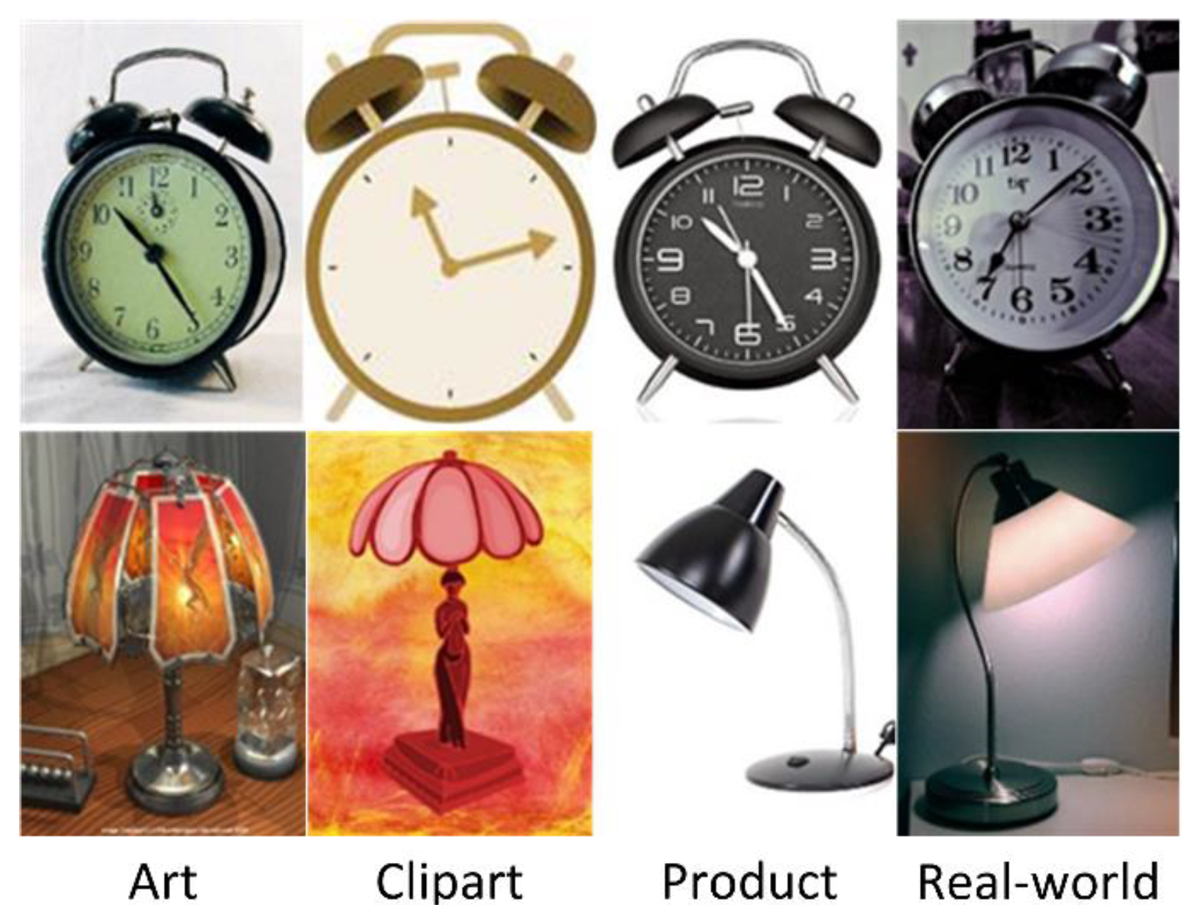
Many domain adaptation (DA) researchers’ [33,35,36] results prove this theory, i.e., for most UDA methods that were tested on an office–home dataset [37], if we set the Real-world as the source domain dataset, then the transfer effect of using Product as the target domain is better than that of using Clipart as the target domain. We can see from the image example in Figure 1 that images that belong to “Real-world” and Product appear to be closer than Clipart. The closer two images are, the smaller the domain distance is, which is more conducive to the transfer of knowledge from source to target domain. In supervised transfer learning, [38,39] also showed the same phenomenon, namely, that the transfer improvements are higher when source and target domain datasets are more similar to each other.
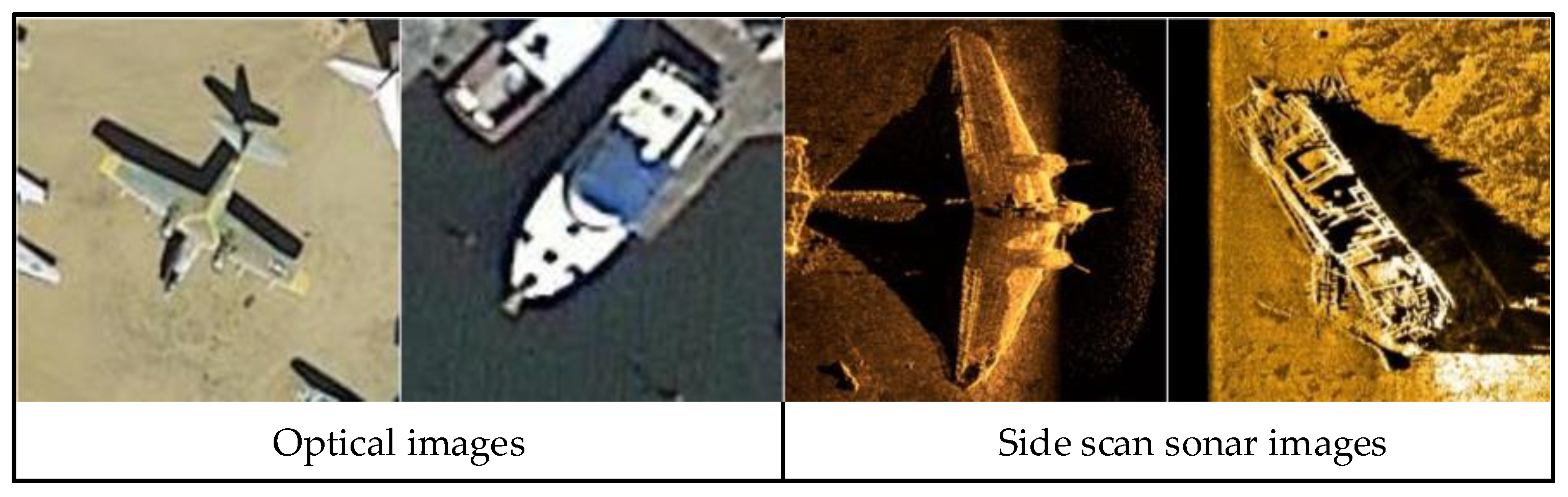
However, as shown in Figure 2, there are great differences between side-scan sonar images and conventional optical images in terms of pixel distribution, texture characteristics and other features; that is, the domain gap is larger than that in the common scenario, which could be why the conventional transfer learning method is usually not particularly effective when it is directly applied to side-scan sonar image classification.
By analyzing the characteristics and the differences between optical image and side-scan sonar image in detail, we find that although the target produces shape deformations in side-scan sonar images, the contour features of the target remain basically unchanged, as in conventional optical images. We can select the contour feature as the domain-invariant feature and take texture features, such as color and pixel value distribution information, as domain-specific features, and by keeping the domain invariant feature, we can make the domain gap narrowed when we take optical image as source domain and side-scan sonar image as target domain. Therefore, we can improve the effectiveness of transfer learning methods.
We formulate our approach as follows: Equation (1) is the classification function, and Equation (2) is the loss function.
where is the input image, which can come from the source or target domain; is the feature extraction network; denotes the feature separation function, which can make the distributions of the source domain features and target domain features closer after feature separation, namely, ; and is the classifier that can complete the mapping between deep features and predictions.
The core element of our method is the feature separation function ; instead of setting up a deep neural network that can learn from data, we use a simpler and more effective method. In our method, is a fixed transformation function, and there are no parameters that need to be learned during the transfer learning stage, which makes it easier to implement. The fixed transformation avoids many problems of the learnable layer, such as the gradient backpropagation problem of the nonlinear transformation layer.
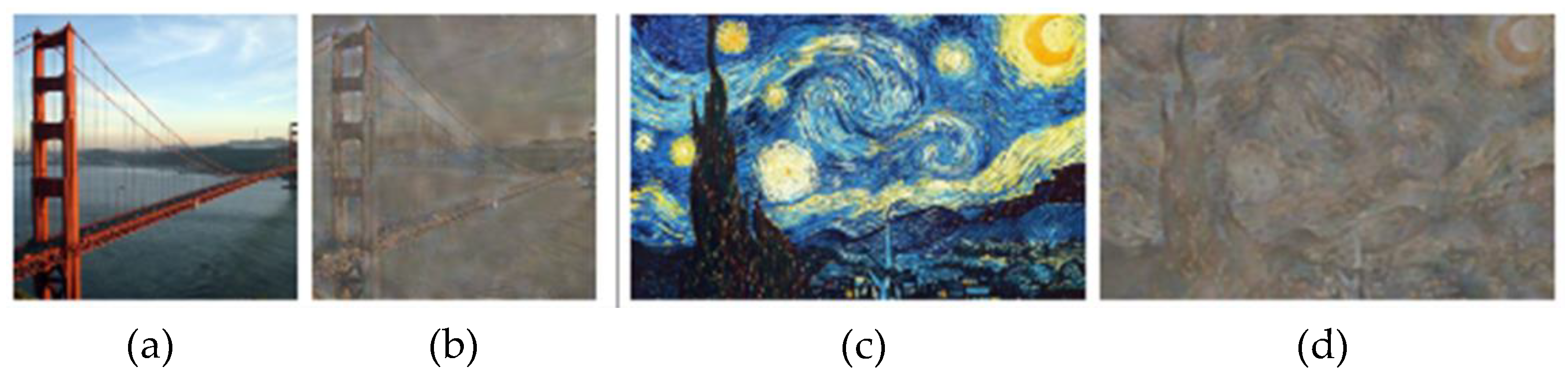
Regarding the feature separation function , our method is inspired by style transfer methods. These methods aim to get an image by imitating another artistic style. Figure 3 shows the effect of image style transfer.
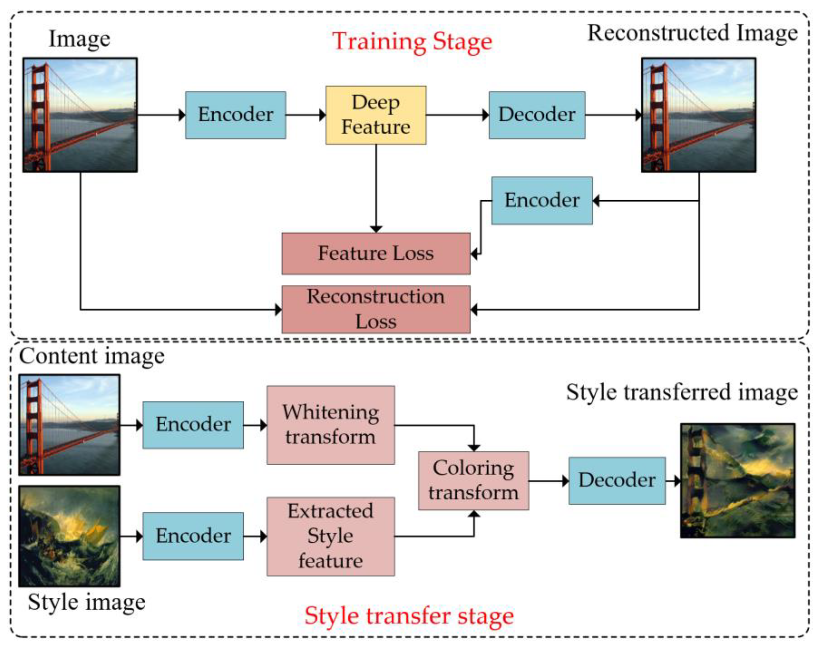
Li et al. [40] proposed a fast and effective style transfer method called PhotoWCT. During the training stage, the PhotoWCT method first trains an autoencoder, and the pixel reconstruction loss [41] and feature loss [42] are used to reconstruct input images during encoder/decoder training.
where and are the input image and reconstructed output, respectively; is an encoder that extracts the deep features; and is a weight parameter.
The style transfer task starts after the autoencoder network training is completed: First, we send the contents image to the encoder of the autoencoder to get content features . Then, we transform the based on Equation (4), which is called the whitening transform.
where is the whitened deep feature, is a diagonal matrix with the eigenvalues of the covariance matrix , and is the corresponding orthogonal matrix of eigenvectors, which satisfies . Then, the style feature extracted from the style image by encoder is combined with the whitened content feature by the coloring transform, which is defined as Equation (5)
where is the colorized feature, is a diagonal matrix with the eigenvalues of the covariance matrix , is the deep feature of style image, and is the corresponding orthogonal matrix of eigenvectors.
Finally, the synthesized image is obtained by feeding the combined deep features into the decoder. Figure 4 shows the network structure of PhotoWCT.
The key strategy behind PhotoWCT is to directly match the feature correlations of the content image to those of the style image via the two projections. In the PhotoWCT method, the whitening step helps peel off the style from an input image while preserving the global content structure, as shown in Figure 5.
In our scenario, we can apply the whitening transform on both the source domain and target domain. The texture features of these two domains are removed, and only the contour features are preserved. Because the reserved features only contain the features of contour information, the domain gap between the source domain and the target domain can be narrowed, and the knowledge transfer efficiency can be improved. The principle of our method is summarized in Formula (6).
However, the whitening transformation cannot remove all style features, and some color features are also retained. When two images have similar styles, there is no obvious difference in style information in the whitened features, so it can effectively narrow the domain gap when the source and target domains are both optical images.
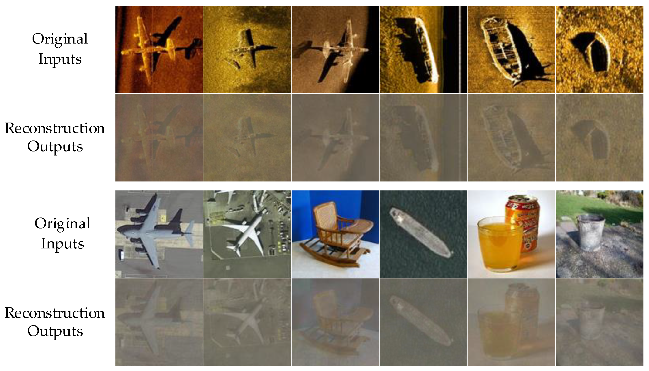
If we directly use the whitening transform as the texture feature removal network to remove texture features of conventional optical images and side-scan sonar images, the effect is not good enough. We visualize the decoded result of the whitened features in Figure 6. We can see that there are still differences in color distribution between the two domains.
To solve this problem, we first analyze the deep feature, and we use the Haar wavelet to decompose the whitened deep feature to observe the frequency band where the color and texture feature appears. If the color and texture features are concentrated in the high frequency band, we can remove the texture features by low-pass filtering the deep features.
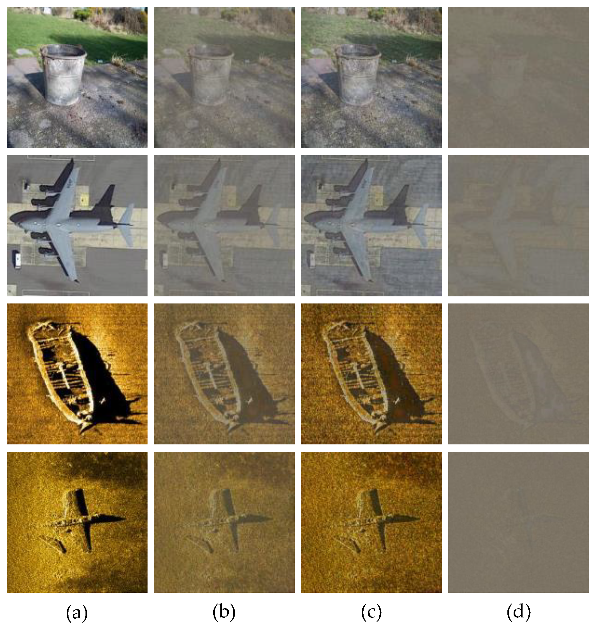
After the deep feature is decomposed, the low-frequency component and high-frequency component are obtained. Since their length is half of the deep feature, we use nearest neighbor interpolation to restore them to the same length as the depth feature. After that, we use the decoder to reconstruct the two decomposed features. Finally, the decode results are shown in Figure 7.
From Figure 7, we can see that, in the reconstruction result of the low frequency component of the whitened deep feature, the color and texture features become clearer, and it can be regarded as the result of low-pass filtering of the whitened depth feature, and after filtering, the domain gap becomes larger; therefore, we do the opposite, which means we add noise to the whitened deep feature, so that the texture features of the output results of the decoder are greatly weakened, which reduces the difference between the source and target domains; that is, the gap between the two domains decreases. Finally, the objective of improving the knowledge transfer efficiency can be achieved.
The effect of the first improvement is shown in Figure 8.
The addition of noise pollution can reduce the domain gap, but the experimental results show that the removal effect of texture features is still insufficient. We find that the main reason is the full use of the un-pooling layer in the decoder of PhotoWCT. Therefore, we propose a second improvement; namely, we alternately use un-pooling and up-sampling layers to enlarge the feature map in the decoder. The basis for improvement is described below.
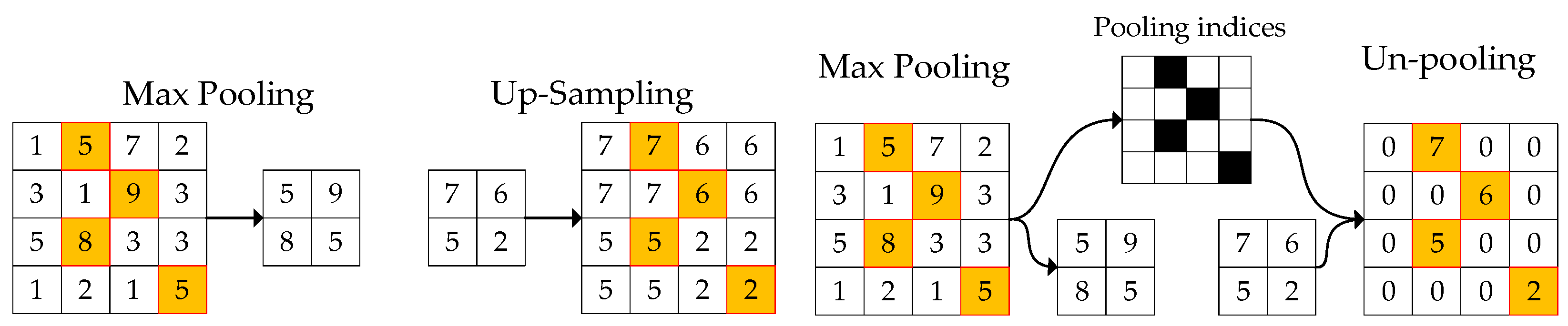
Different from the traditional commonly used up-sampling layer, the un-pooling layer takes the saved locations of maximum activations during the pooling operation as indicators and uses them to place each activation back in its original pooled location. This un-pooling strategy could help preserve information in the reconstruction task [43]. As a result, the texture information is retained through the maximum activation value position indicator of max-pooling.
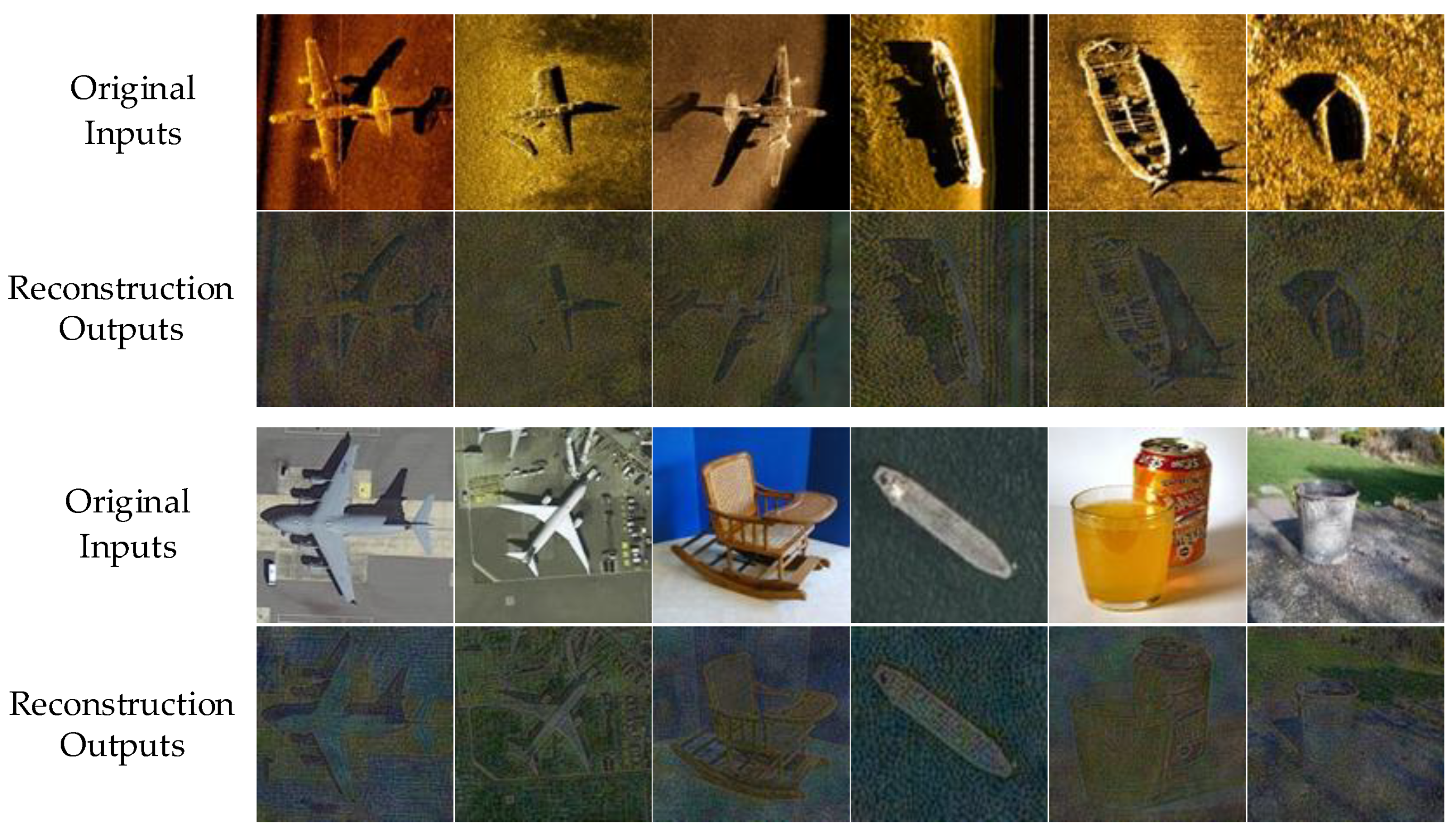
To prove this, we use pure noise as a deep feature to feed into the decoder. Since the noise is generated randomly, it does not contain any image information; therefore, if the reconstruction result still contains information of the original input image, it must be carried by the maximum activation value position indicator. The test results are shown in Figure 9.
From Figure 9 we can see that when using the unpooling layer, even if we use pure noise as a deep feature, the reconstructed output still contains much information from the original input. Additionally, we further find that during the unpooling operation, if we enlarge the feature activation value, which fed into the unpooling layer, the reconstructed output image of the decoder will be closer to the original input image, even if the input of the decoder is still pure noise.
Because of the use of the un-pooling layer, too much information is preserved, which deviates from our original intention; thus, we use a traditional up-sampling layer in the appropriate position, and the up-sampling layer enlarges the feature map in a way that ignores the active position, which could damage the feature information transmission, which is what we need. The operating processes of the up-sampling and un-pooling layers are illustrated in Figure 10.
Generally, for an encoder, the shallow layer of the neural network usually extracts local detailed texture and color features, while the deeper layer extracts more abstract information, such as contour and size. Then, for the decoder, which is designed to be symmetrical to the encoder, the shallow layer usually reconstructs abstract global contour features, and the deeper layer reconstructs detailed texture and color features. Therefore, we place the up-sampling layer at the deeper layer, and the un-pooling layer is still used on the shallow layer to preserve the contour information and remove the texture information at the same time.
Finally, after two improvements, the removal effect of texture features is shown in Figure 11.
Finally, our network structure is illustrated in Figure 12. In the next section, we carry out many comparative experiments to verify our proposed method.
3. Results
We verify our proposed method by conducting experiments on the side-scan sonar image classification task and the forward-looking sonar image target detection task. For the experiments on the side-scan sonar image classification task, we also use the supervised transfer learning method and unsupervised transfer learning method to evaluate the effectiveness.
3.1. Supervised Transfer Learning Experiments of the Side-Scan Sonar Image Classification Task
3.1.1. Source Domain Dataset
Because the visual angles of remote sensing images and side-scan sonar images are similar, the domain gap will be smaller after removing texture features, which is more conducive to the transfer of knowledge; thus, we select several remote sensing image datasets as the source domain datasets, namely DOTA [44] UCAS-AOD [45], NWPU VHR-10 [46], RSOD-Dataset [47], and NWPU RESISC45 [48].
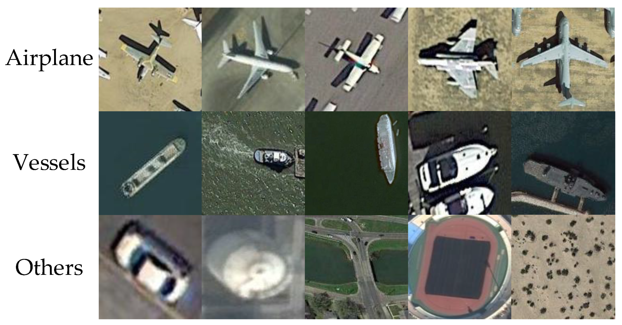
As four of them are designed for detection tasks, we cut their images into image pieces based on the provided bounding boxes. Then, we filter out small image pieces and randomly delete some pieces to ensure the approximate balance of the dataset. Finally, the constructed source domain dataset contains three categories: aircraft (1313 samples), ship (601 samples), and others (2080 samples). The ‘others’ category consists of samples from the five datasets that do not correspond to aircrafts or ships, including trucks, cars, overpasses, beaches, etc.
The reason for this construction is that the source domain and the target domain could share the same label space, that is, ; in this way, we can use the dataset to measure the effectiveness of our method on different problems, such as supervised transfer learning and unsupervised transfer learning tasks. Examples from the source domain dataset are shown in Figure 13.
3.1.2. Side-Scan Sonar Image Dataset
For the side-scan sonar image dataset, we collect 33 images of aircrafts, 179 images of shipwrecks, and 265 other images that belong to 12 categories, such as rocks, buckers and fishing boxes. We merge them because the numbers of samples in those categories are too small, especially for the supervised transfer learning task. We also select some samples as the test set. For example, there are only eight samples in the fishing box category, and only two samples are taken as the test samples. It is difficult to effectively measure the effectiveness of the algorithm on such a small test sample. Therefore, we combine them as negative samples, namely, samples that do not correspond to aircrafts or shipwrecks. Examples from the target domain dataset are shown in Figure 14.
3.1.3. Supervised Transfer Learning Experiments
Among the many supervised transfer learning methods, the simplest and most effective is fine-tune [49], which was also widely used in many areas. The core principle of fine-tuning is that if we have a neural network that was well trained using a source domain dataset for the source task, we can freeze (or share) most of its layers and only train the last few layers using a target domain dataset to produce a target network, namely, a fine-tuned network. Because of its simplicity and easy implementation, we use the fine-tuning method in the supervised transfer learning experiment. We first train an encoder and a decoder using the ImageNet dataset. Then, we embed the trained encoder and decoder into our proposed method and freeze the weights of the encoder and decoder. Next, we use the source domain dataset to train the classification network and, finally, use the target domain dataset to fine-tune this classification network. The effectiveness of this method is measured by evaluating the classification accuracy.
In TFRN, as for PhotoWCT, we use the feature extraction part of VGG-19 [50] as the encoder, and we use the inverse of the encoder as the decoder. During the training stage, we use the ImageNet dataset as input data. The training goal is to restore the features extracted by the encoder to the input image as much as possible. The pixel reconstruction loss [41] and feature loss [42] are adopted as described before. After the encoder is well trained, we extract it and embed it into our proposed method. At the same time, we freeze the weights of the encoder and decoder, making the texture feature removal network a fixed transformation process without dynamic adjustment.
The output of the TFRN is input into a classification network. For this classification network, we use ResNet-50 [51] as a backbone network. When training the data classification network in the source domain, we train the classification network from scratch, while in fine-tuning, we test and fine-tune all parameters and the last two layers to better evaluate the effectiveness of the improved method.
In the process of fine-tuning the source domain data classification network for the target domain, we randomly select 70% of the dataset of the target domain as the training set and the remaining 30% of the samples as the validation set. The validation set does not participate in the training process and is only used to evaluate the network classification ability.
To better verify the method proposed in this paper, we conduct two comparative experiments. In the first experiment, the target domain dataset is used directly to train the classification network without the transfer learning method. We denote this classification network . In the second experiment, we simply use the basic fine-tuning method without adding the texture feature removal network. We use the optical remote sensing image dataset as the source domain to train the classification network and then directly use the side-scan sonar image dataset as the target domain to fine-tune the source domain classification network. This classification network is denoted as . Finally, due to the large deviation in the number of samples among the three categories, to better measure the classification ability of the classification network, we measure the global accuracy and mean accuracy at the same time.
The mean accuracy and global accuracy are measured using Equations (8) and (9), respectively.
The experimental results are presented in Table 1.
The classification results of (without the transfer learning method) are very poor, and there is a great difference between the average accuracy and the global accuracy. Only 6 aircraft samples and 45 shipwreck samples are correctly classified, while most of the samples in the other categories are correctly classified, which indicates that the network has a substantial classification bias. We statistically analyze the predicted results of all test samples and find that the network classifies almost all samples into the other category, that is, the network does not have satisfactory classification ability.
performs better, 9 aircraft samples and 67 wreck category samples are correctly classified, and the global accuracy is close to the mean accuracy, which also confirms the effectiveness of the fine-tuning method.
Our method achieves excellent results. With the TFRN, 11 of 13 real aircraft SSS images are correctly recognized, and 66 of 71 real shipwreck SSS images are recognized. The mean and global accuracies are closer than those of , and the classification ability is well balanced for all test categories.
We also plot some classification results on the validation set in Figure 15, and we observe that, in the classification samples that are incorrectly classified as belonging to the ship category, only the general outline of the ship is visible, while other parts are messy and have no shadow. These samples are quite different from most samples of the ship category, so they are easily misclassified into other categories. The samples of the other category that are incorrectly classified have contour shapes that are close to those of the samples of the ship or aircraft category. These results reveal that the classification network does use appropriate features as the classification basis.
3.2. Unsupervised Transfer Learning Experiment on the Side-Scan Sonar Image Classification Task
As a special case of transfer learning, the unsupervised domain adaptation (UDA) method usually learns a classifier, which can address the situation where there are labeled source data and the target domain has accessible samples but no labels [52]. Because of its ability to learn from labeled data and apply the learning results to a similar domain, UDA can reduce the need for costly labeled data in the target domain; therefore, it was widely used in natural language processing, machine translation, computer vision, and other application scenarios [53].
Among many UDA methods, DaNN [54] is a very ingenious and deep neural network-based UDA method. DaNN was the first to introduce adversarial training into the field of UDA, and a domain classifier was added to the traditional classification network. In the training stage, the source domain training samples and the target domain training samples are mixed as the input of the network. The conventional classification network is trained by using the source domain dataset, and the domain classifier is designed to distinguish whether the training samples come from the source domain or the target domain.
The common idea is that with the training of the network, the prediction of the source domain becomes increasingly accurate, and at the same time, the domain classifier can accurately distinguish the source of each sample. Based on this conventional idea, DaNN uses a gradient inversion layer at the beginning of the domain classifier. By inverting the gradient calculated by the domain classifier, the DNN is optimized toward the positive gradient direction, which means the loss of the domain classifier increases, leading to the domain classifier becoming increasingly inaccurate, which also means the DNN becomes unable to distinguish the source of input data.
When the deep network cannot distinguish whether the sample comes from the source domain or the target domain, for the classifier, the source domain and target domain are the same; namely, there is no domain gap between the source domain and the target domain. Because there is no domain gap, the classifier trained by the source domain can be applied to classify samples from the target domain. This is the key idea of DaNN. For the UDA experiment, we use DaNN as the basic network and combine our TFRN with DaNN.
The datasets used in the UDA transfer learning experiment are the same as those used in the supervised transfer learning experiment. The texture feature removal network part is also the same as that in supervised transfer learning, which was described in Section 3.1.3. We connect the DaNN network with our TFRN.
We reproduce the code for DaNN in PyTorch, and the backbone network is ResNet-101 [51]. We use two liner layers as domain classifiers. At the top of the classifier, we add a gradient inversion layer, which does not perform any calculation during forward propagation, and multiply the gradient by -1 during error backpropagation to realize gradient inversion.
For the source domain classifier, we use cross entropy as the loss function, and for the domain classifier, we use the L2 norm as the domain loss. The final loss function is presented as Equation (10), where λ is the weight parameter.
In the setting of the UDA problem, the samples of the target domain are accessible but have no labels; therefore, we use all the samples of side-scan sonar images in the training, and after the network is fully trained, we use all the side-scan sonar images to evaluate the classification ability of the network. As in Section 3.1.3, we still evaluate the global accuracy and mean accuracy.
We compare these values with those of the original DaNN to verify the improvement in classification ability after adding TFRN. The UDA experimental results are presented in Table 2.
According to Table 2, after adding the TFRN, the classification mean accuracy is greatly improved, and the global accuracy and mean accuracy are closer, which proves that the method proposed in this paper can effectively address the situation of large differences between the distributions of the target domain and source domain.
3.3. Imaging Sonar Object Detection Experiments and Results
3.3.1. Dataset
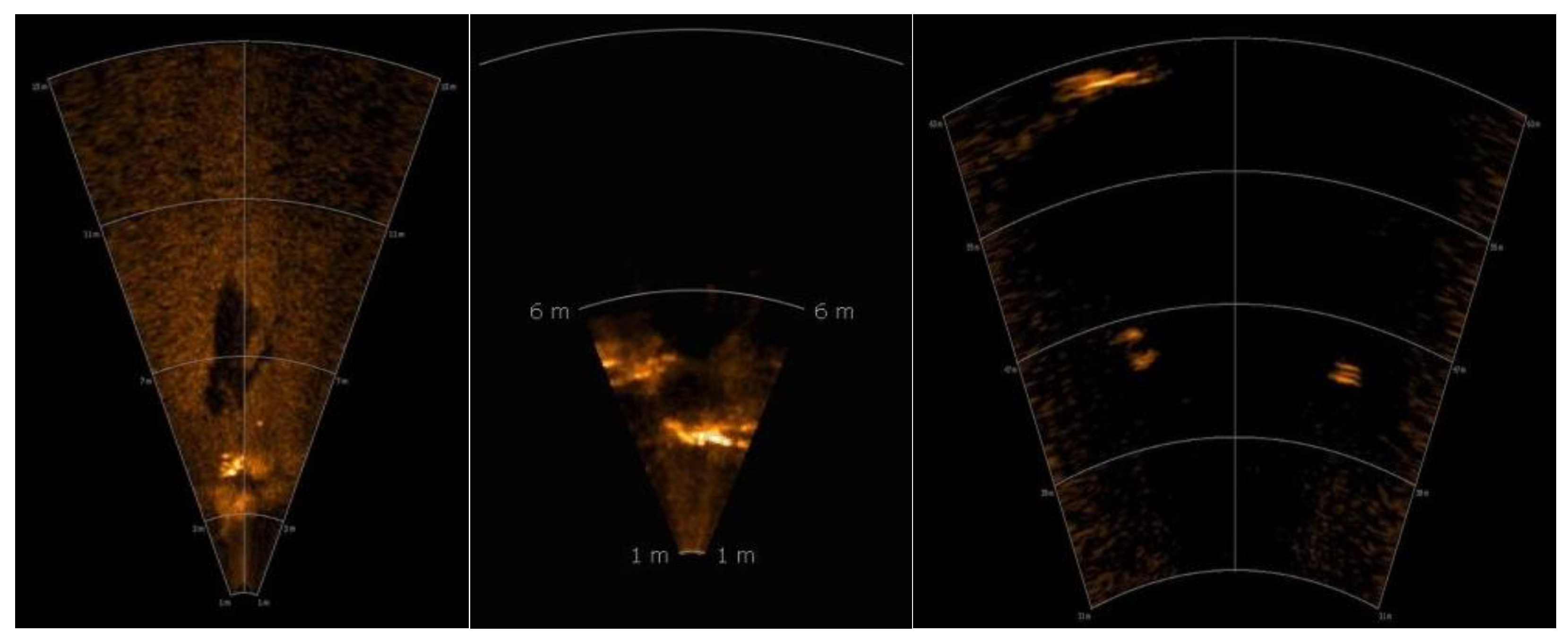
We also evaluate the proposed method in the target detection task of forward-looking sonar (FLS) images, which are widely used in underwater vehicles [3].
A total of 42 forward-looking sonar images were collected, of which 10 are randomly selected as test samples and the remaining 32 as training samples. Our FLS datasets only include one category, namely, diver. Examples of FLS datasets are shown in Figure 16.
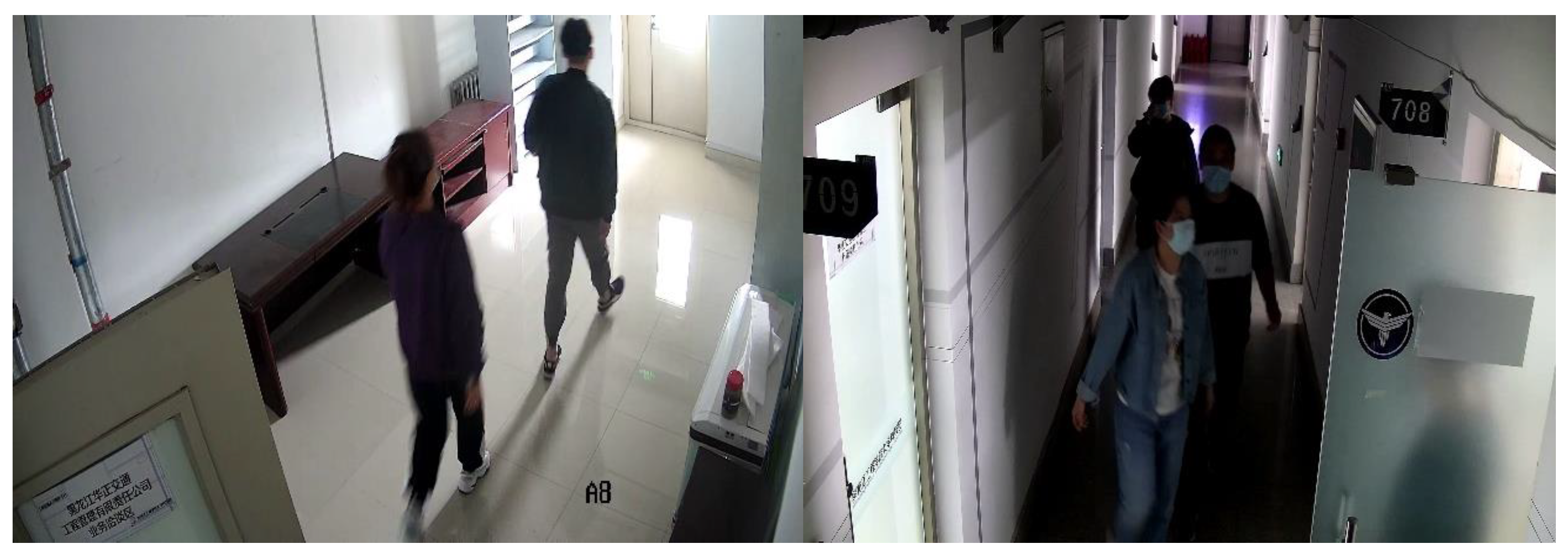
We also construct a corresponding source domain dataset for forward-looking sonar images and collect a total of 372 images. All images are captured by surveillance cameras, and the images only contain one category, which is consistent with the FLS dataset. Examples are shown in Figure 17.
3.3.2. Forward-Looking Sonar Image Detection Experiments
For the experiments, we use a setting similar with that in Section 3.1. Two comparative experiments are conducted. In the first experiment, the detection network is trained directly using the FLS dataset without using the transfer learning method, and we denote the detection network . In the second experiment, the fine-tune method is used. We first train a source domain detection DNN using the source domain dataset. After that, we use the FLS dataset to fine-tune the source domain detection DNN, and we denote the detection network . In our method, we put the proposed TFRN before the detection network, and the other settings are the same as those of . We use CenterNet [55] as the detection DNN, which is an excellent anchor-free object detection framework, and we use ResNet-18 [51] as the backbone feature extractor in CenterNet. The input resolution is 640 × 480, the initial learning rate is set to 1e-4, and we train the network for 200 epochs, with the learning rate dropping by 10× at 120 epochs. The hyperparameters are all the same in every experimental step.
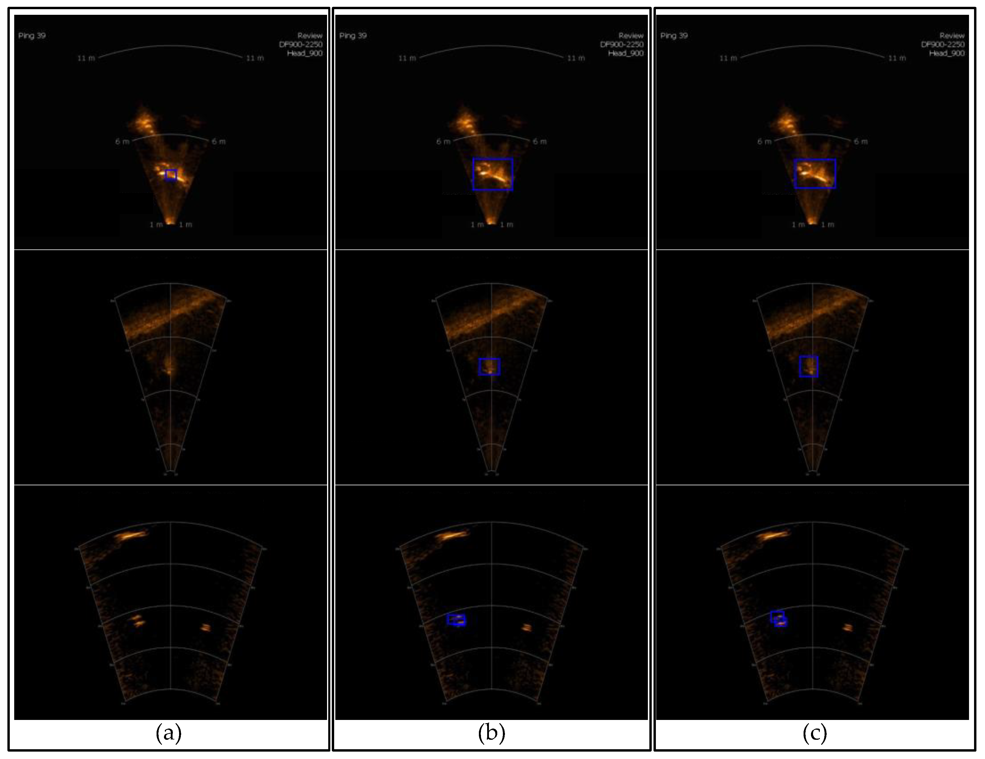
We use the average precision (AP) [56] over all IOU thresholds () and the AP at an IOU threshold of 0.5 () to measure the object detection ability of the network. Since there are only 10 test samples, we can easily count the number of incorrect and missed detections. The results are reported in Table 3, and Figure 18 shows some detection results from the three experiments.
We can see that, if we directly use a small number of target domain data sets to train the detection network, the bounding box of the detection results is very inaccurate, and there are many wrong detections and missing detections. With the use of the transfer learning method, and were significantly improved, and the number of error detections and missing detections was reduced, leading to the fact that the similarity between the source domain and the target domain is positively correlated with the transfer effect.
However, after using our TFRN, the domain gap between source domain and target domain is further reduced by the removal of texture features, AP is further improved, and the bounding box regression is more accurate. There is only one wrong detection in 10 test samples, these results prove that out method is not only effective in side-scan-sonar images, but also in forward-looking-sonar image target detection tasks.
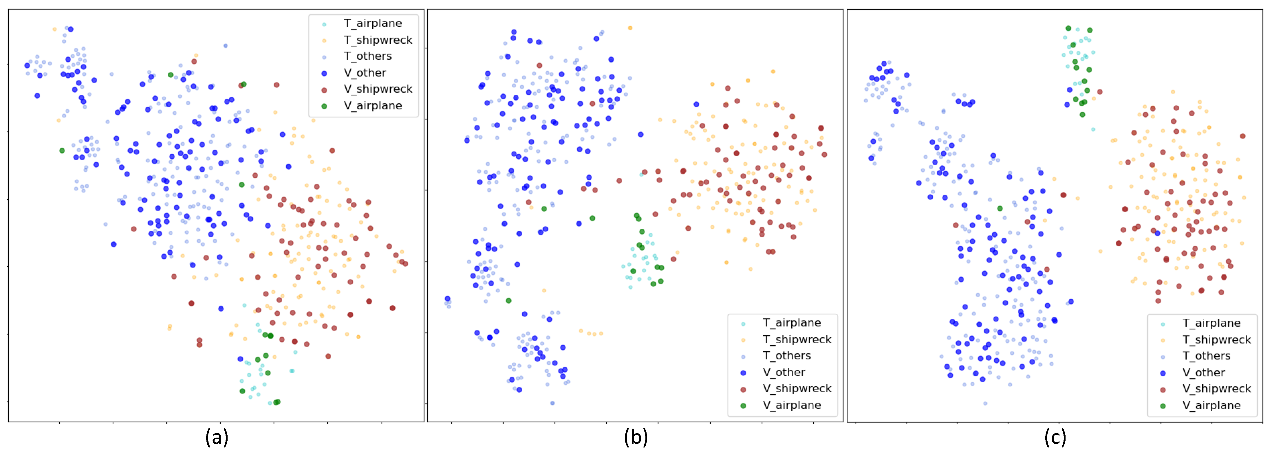
We further use the t-distributed stochastic neighbor embedding [57] method to reduce the dimensions of features and display them; t-SNE is a technique for dimensionality reduction that is particularly well suited for the visualization of high-dimensional features. If two domain features are in close proximity to each other, then the features after reducing the dimensions are also close, and we can evaluate the effectiveness of our proposed method by analyzing the distributions of low-dimensional features between the two domains.
We first visualize the deep features in side-scan sonar-supervised transfer learning experiments. The deep features are extracted from the last residual block of the classification network. We only present the feature distribution of the target domain, and the training set and test set are represented by different marks to intuitively reflect the generalization ability of the network. We also compare the feature distribution results of and . The results are plotted in Figure 19.
As shown in Figure 18a, the distribution of the test set is very different from that of the training set, which shows that the network suffers from overfitting. Due to training on too few samples, the network learns the wrong characteristics; hence, the test set cannot be classified correctly. In Figure 18b, the network shows no overfitting, the distributions of the training set and test set are basically the same, and the network demonstrates classification ability. The results in Figure 18c are better than those in Figure 18b. The distribution range of the test set is smaller, and the inter class distance of the features is larger, which shows that after the texture feature removal network is applied, the main network can effectively extract the most critical features for classification.
4. Discussion
In this article, we focused on the problem that the conventional transfer learning method may not be suitable for the situation where the source domain is quite different from the target domain, such as when the source domain consists of conventional optical images and the target domain consists of sonar images. Conventional transfer learning methods would fail because of the huge domain gap.
We assumed that the image features are composed of domain-invariant features and domain-specific features, and that the domain-specific features are the texture features of the images. Domain-invariant features are the features contained in both domains. If we only use domain-invariant features as the classification basis, then in DNN’s view, there is no domain gap. Therefore, the DNN trained using the source domain data can also be used in the target domain.
The core of our method is to narrow the domain gap between the two domains at the sample level, while the whitening transformation is the closest technique to achieve texture feature removal.
Since the effect of directly applying the whitening transform is not ideal, we analyze the depth features after whitening, and look forward to further removing texture features by filtering; however, the Haar wavelet decomposition results show that after filtering out high-frequency components, texture features are enhanced. This leads to the first improvement, adding noise pollution to the whitened deep features.
In order to further reduce the difference between the two domains, we propose a second improvement. By using the noise without any information as the deep feature, we successfully found that the pooling indicator carries the texture feature, so we used a nearest neighbor up-sampling layer in the decoder to cut off this feature transfer channel.
After two improvements, the pixel value distribution and noise level of the source and target images processed by the texture feature removal network are relatively close, and they look more similar; therefore, the domain gap between the source domain and the target domain can be greatly narrowed, which leads to better performance improvements in transfer learning.
After carefully designing the texture feature removal network, we compared our method to conventional transfer learning methods using datasets that we built, and the results of both side-scan sonar image classification transfer learning experiments and forward-looking sonar object detection experiments show that our method can effectively improve the accuracy of classification. The research that was reported in this paper promotes the practical application value of transfer learning in the field of special small-sample image classification tasks.
Author Contributions
Conceptualization, C.L. and X.Y.; methodology, C.L. and X.Y.; software, C.L.; validation, C.L., J.X. and X.Y.; formal analysis, X.Y.; investigation, C.L., Y.J. and X.Y.; resources, C.L. and X.Y.; data curation, C.L., J.X. and Y.J.; writing—original draft preparation, C.L.; writing—review and editing, C.L. and X.Y.; visualization, C.L., J.X. and Y.J.; supervision, X.Y.; project administration, X.Y.; funding acquisition, X.Y. All authors have read and agreed to the published version of the manuscript.
Funding
This work was supported by the National Natural Science Foundation of China (Grant No. 42276187 and No. 41876100) and the Fundamental Research Funds for the Central Universities(Grant No. 3072022FSC0401).
Data Availability Statement
All the experiments data and code can be found in https://github.com/guizilaile23/TFRN (accessed on 3 January 2023).
Acknowledgments
We would like to thank the editor and the anonymous reviewers for their valuable comments and suggestions that greatly improve the quality of this paper.
Conflicts of Interest
The authors declare no conflict of interest.
References
- Huo, G.; Wu, Z.; Li, J. Underwater Object Classification in Sidescan Sonar Images Using Deep Transfer Learning and Semisynthetic Training Data. IEEE Access 2020, 8, 47407–47418. [Google Scholar] [CrossRef]
- Ye, X.; Yang, H.; Li, C.; Jia, Y.; Li, P. A gray scale correction method for side-scan sonar images based on retinex. Remote Sens. 2019, 11, 1281. [Google Scholar] [CrossRef] [Green Version]
- Song, Y.; He, B.; Liu, P. Real-Time Object Detection for AUVs Using Self-Cascaded Convolutional Neural Networks. IEEE J. Ocean. Eng. 2021, 46, 56–67. [Google Scholar] [CrossRef]
- Cho, H.; Gu, J.; Yu, S. Robust Sonar-Based Underwater Object Recognition Against Angle-of-View Variation. IEEE Sens. J. 2016, 16, 1013–1025. [Google Scholar] [CrossRef]
- Li, C.; Ye, X.; Cao, D.; Hou, J.; Yang, H. Zero shot objects classification method of side scan sonar image based on synthesis of pseudo samples. Appl. Acoust. 2021, 173, 107691. [Google Scholar] [CrossRef]
- Xu, H.; Yuan, H. An svm-based adaboost cascade classifier for sonar image. IEEE Access 2020, 8, 115857–115864. [Google Scholar] [CrossRef]
- Zhuang, F.; Qi, Z.; Duan, K.; Xi, D.; Zhu, Y.; Zhu, H.; Xiong, H.; He, Q. A comprehensive survey on transfer learning. Proc. IEEE 2021, 109, 43–76. [Google Scholar] [CrossRef]
- Talo, M.; Baloglu, U.B.; Yildrm, Ö.; Rajendra Acharya, U. Application of deep transfer learning for automated brain abnormality classification using mr images. Cogn. Syst. Res. 2019, 54, 176–188. [Google Scholar] [CrossRef]
- Swati, Z.N.K.; Zhao, Q.; Kabir, M.; Ali, F.; Ali, Z.; Ahmed, S.; Lu, J. Brain tumor classification for mr images using transfer learning and fine-tuning. Comput. Med. Imaging Graph. 2019, 75, 34–46. [Google Scholar] [CrossRef]
- Rahman, T.; Chowdhury, M.E.H.; Khandakar, A.; Islam, K.R.; Islam, K.F.; Mahbub, Z.B.; Kadir, M.A.; Kashem, S. Transfer learning with deep convolutional neural network (cnn) for pneumonia detection using chest X-ray. Appl. Sci. 2020, 10, 3233. [Google Scholar] [CrossRef]
- Lu, S.; Lu, Z.; Zhang, Y. Pathological brain detection based on alexnet and transfer learning. J. Comput. Sci. 2019, 30, 41–47. [Google Scholar] [CrossRef]
- Liang, G.; Zheng, L. A transfer learning method with deep residual network for pediatric pneumonia diagnosis. Comput. Methods Programs Biomed. 2020, 187, 104964. [Google Scholar] [CrossRef] [PubMed]
- Khan, S.; Islam, N.; Jan, Z.; Din, I.U.; Rodrigues, J.J.C. A novel deep learning based framework for the detection and classification of breast cancer using transfer learning. Pattern Recognit. Lett. 2019, 125, 1–6. [Google Scholar] [CrossRef]
- Chouhan, V.; Singh, S.K.; Khamparia, A.; Gupta, D.; Tiwari, P.; Moreira, C.; Damaeviius, R.; De Albuquerque, V.H.C. A novel transfer learning based approach for pneumonia detection in chest X-ray images. Appl. Sci. 2020, 10, 559. [Google Scholar] [CrossRef] [Green Version]
- Lumini, A.; Nanni, L. Deep learning and transfer learning features for plankton classification. Ecol. Inform. 2019, 51, 33–43. [Google Scholar] [CrossRef]
- Coulibaly, S.; Kamsu-Foguem, B.; Kamissoko, D.; Traore, D. Deep neural networks with transfer learning in millet crop images. Comput. Ind. 2019, 108, 115–120. [Google Scholar] [CrossRef] [Green Version]
- Chen, J.; Chen, J.; Zhang, D.; Sun, Y.; Nanehkaran, Y. Using deep transfer learning for image-based plant disease identification. Comput. Electron. Agric. 2020, 173, 105393. [Google Scholar] [CrossRef]
- Qin, X.; Luo, X.; Wu, Z.; Shang, J. Optimizing the sediment classification of small side-scan sonar images based on deep learning. IEEE Access 2021, 9, 29416–29428. [Google Scholar] [CrossRef]
- Pires de Lima, R.; Marfurt, K. Convolutional neural network for remote-sensing scene classification: Transfer learning analysis. Remote Sens. 2019, 12, 86. [Google Scholar] [CrossRef] [Green Version]
- You, K.; Liu, Y.; Wang, J.; Long, M. Logme: Practical assessment of pre-trained models for transfer learning. In Proceedings of the 38th International Conference on Machine Learning, Virtual Event, 18–24 July 2021; Volume 139, pp. 12133–12143. [Google Scholar]
- You, K.; Kou, Z.; Long, M.; Wang, J. Co-tuning for transfer learning. Adv. Neural Inf. Process. Syst. 2020, 33, 17236–17246. [Google Scholar]
- Guo, Y.; Shi, H.; Kumar, A.; Grauman, K.; Rosing, T.; Feris, R. Spottune: Transfer learning through adaptive fine-tuning. In Proceedings of the IEEE/CVF Conference on Computer Vision and Pattern Recognition (CVPR), Long Beach, CA, USA, 16–20 June 2019; pp. 4805–4814. [Google Scholar]
- Shafahi, A.; Saadatpanah, P.; Zhu, C.; Ghiasi, A.; Studer, C.; Jacobs, D.; Goldstein, T. Adversarially robust transfer learning. arXiv 2019, arXiv:1905.08232. [Google Scholar]
- Chen, W.; Liu, Z.; Zhang, H.; Chen, M.; Zhang, Y. A submarine pipeline segmentation method for noisy forward-looking sonar images using global information and coarse segmentation. Appl. Ocean Res. 2021, 112, 102691. [Google Scholar] [CrossRef]
- Yulin, T.; Shaohua, J.; Gang, B.; Yonzhou, Z.; Fan, L. Wreckage target recognition in side-scan sonar images based on an improved faster r-cnn model. In Proceedings of the 2020 International Conference on Big Data & Artificial Intelligence & Software Engineering (ICBASE), Bangkok, Thailand, 30 October–1 November 2020; pp. 348–354. [Google Scholar]
- Zhou, Y.; Chen, S. Research on lightweight improvement of sonar image classification network. In Proceedings of the Journal of Physics: Conference Series, Dali, China, 18–20 June 2021; p. 012140. [Google Scholar]
- Yu, Y.; Zhao, J.; Gong, Q.; Huang, C.; Zheng, G.; Ma, J. Real-time underwater maritime object detection in side-scan sonar images based on transformer-yolov5. Remote Sens. 2021, 13, 3555. [Google Scholar] [CrossRef]
- Chandrashekar, G.; Raaza, A.; Rajendran, V.; Ravikumar, D. Side scan sonar image augmentation for sediment classification using deep learning based transfer learning approach. Mater. Today Proc. 2021, 1, 1. [Google Scholar] [CrossRef]
- Ochal, M.; Vazquez, J.; Petillot, Y.; Wang, S. A comparison of few-shot learning methods for underwater optical and sonar image classification. In Proceedings of the Global Oceans 2020, Singapore U.S., Gulf Coast, Biloxi, MS, USA, 5–30 October 2020; pp. 1–10. [Google Scholar]
- Ghifary, M.; Kleijn, W.B.; Zhang, M. Domain adaptive neural networks for object recognition. In Proceedings of Pacific Rim International Conference on Artificial Intelligence; Springer: Cham, Switzerland, 2014; pp. 898–904. [Google Scholar]
- Long, M.; Zhu, H.; Wang, J.; Jordan, M.I. Deep transfer learning with joint adaptation networks. In Proceedings of the 34th International Conference on Machine Learning, Sydney, Australia, 6–11 August 2017; Volume 70, pp. 2208–2217. [Google Scholar]
- Zhuang, F.; Cheng, X.; Luo, P.; Pan, S.J.; He, Q. Supervised representation learning with double encoding-layer autoencoder for transfer learning. ACM Trans. Intell. Syst. Technol. 2017, 9, 1–17. [Google Scholar] [CrossRef]
- Wang, J.; Lan, C.; Liu, C.; Ouyang, Y.; Qin, T.; Lu, W.; Chen, Y.; Zeng, W.; Yu, P. Generalizing to unseen domains: A survey on domain Generalization. IEEE Trans. Knowl. Data Eng. 2022, 1, 1. [Google Scholar] [CrossRef]
- Gatys, L.; Ecker, A.S.; Bethge, M. Texture synthesis using convolutional neural networks. Adv. Neural Inf. Process. Syst. 2015, 28, 262–270. [Google Scholar]
- Cui, S.; Wang, S.; Zhuo, J.; Li, L.; Huang, Q.; Tian, Q. Towards discriminability and diversity: Batch nuclear-norm maximization under label insufficient situations. In Proceedings of the IEEE/CVF Conference on Computer Vision and Pattern Recognition, Virtual Event, 14–19 June 2020; pp. 3941–3950. [Google Scholar]
- Xu, T.; Chen, W.; Wang, P.; Wang, F.; Li, H.; Jin, R. Cdtrans: Cross-domain transformer for unsupervised domain adaptation. arXiv 2021, arXiv:2109.06165. [Google Scholar]
- Venkateswara, H.; Eusebio, J.; Chakraborty, S.; Panchanathan, S. Deep hashing network for unsupervised domain adaptation. In Proceedings of the IEEE Conference on Computer Vision and Pattern Recognition (CVPR), Honolulu, HI, USA, 21–26 July 2017; pp. 5018–5027. [Google Scholar]
- Yosinski, J.; Clune, J.; Bengio, Y.; Lipson, H. How transferable are features in deep neural networks? Adv. Neural Inf. Process. Syst. 2014, 27, 1. [Google Scholar]
- Long, M.; Cao, Y.; Wang, J.; Jordan, M. Learning transferable features with deep adaptation networks. In Proceedings of the International Conference on Machine Learning, Lille, France, 6–11 July 2015; Volume 37, pp. 97–105. [Google Scholar]
- Li, Y.; Liu, M.; Li, X.; Yang, M.; Kautz, J. A closed-form solution to photorealistic image stylization. In Proceedings of the European Conference on Computer Vision (ECCV), Munich, Germany, 8–14 September 2018; pp. 453–468. [Google Scholar]
- Alexey, D.; Thomas, B. Generating images with perceptual similarity metrics based on deep networks. Adv. Neural Inf. Process. Syst. 2016, 29, 658–666. [Google Scholar]
- Johnson, J.; Alahi, A.; Fei-Fei, L. Perceptual losses for real-time style transfer and super-resolution. In Proceedings of the European Conference on Computer Vision (ECCV), Amsterdam, The Netherlands, 8–16 October 2016; pp. 694–711. [Google Scholar]
- Noh, H.; Hong, S.; Han, B. Learning deconvolution network for semantic segmentation. In Proceedings of the 2015 IEEE International Conference on Computer Vision (ICCV), Santiago, Chile, 7–13 December 2015; pp. 1520–1528. [Google Scholar]
- Xia, G.; Bai, X.; Ding, J.; Zhu, Z.; Belongie, S.; Luo, J.; Datcu, M.; Pelillo, M.; Zhang, L. Dota: A large-scale dataset for object detection in aerial images. In Proceedings of the IEEE Conference on Computer Vision and Pattern Recognition (CVPR), Salt Lake City, UT, USA, 18–22 June 2018; pp. 3974–3983. [Google Scholar]
- Zhu, H.; Chen, X.; Dai, W.; Fu, K.; Ye, Q.; Jiao, J. Orientation robust object detection in aerial images using deep convolutional neural network. In Proceedings of the 2015 IEEE International Conference on Image Processing (ICIP), Quebec, QC, Canada, 27–30 September 2015; pp. 3735–3739. [Google Scholar]
- Cheng, G.; Han, J. A survey on object detection in optical remote sensing images. Isprs J. Photogramm. Remote Sens. 2016, 117, 11–28. [Google Scholar] [CrossRef] [Green Version]
- Long, Y.; Gong, Y.; Xiao, Z.; Liu, Q. Accurate object localization in remote sensing images based on convolutional neural networks. IEEE Trans. Geosci. Remote Sens. 2017, 55, 2486–2498. [Google Scholar] [CrossRef]
- Gong, C.; Han, J.; Lu, X. Remote sensing image scene classification: Benchmark and state of the art. Proc. IEEE 2017, 105, 1865–1883. [Google Scholar]
- Yin, X.; Chen, W.; Wu, X.; Yue, H. Fine-tuning and visualization of convolutional neural networks. In Proceedings of the 12th IEEE Conference on Industrial Electronics and Applications (ICIEA), Siem Reap, Cambodia, 18–20 June 2017; pp. 1310–1315. [Google Scholar]
- Karen, S.; Andrew, Z. Very deep convolutional networks for large-scale image recognition. arXiv 2014, arXiv:1409.1556. [Google Scholar]
- He, K.; Zhang, X.; Ren, S.; Sun, J. Deep residual learning for image recognition. In Proceedings of the 2016 IEEE Conference on Computer Vision and Pattern Recognition (CVPR), Las Vegas, NY, USA, 26 June–1 July 2016; pp. 770–778. [Google Scholar]
- Zhao, S.; Yue, X.; Zhang, S.; Li, B.; Zhao, H.; Wu, B.; Krishna, R.; Gonzalez, J.E.; Sangiovanni-Vincentelli, A.; Seshia, S.A.; et al. A review of single-source deep unsupervised visual domain adaptation. IEEE Trans. Neural Netw. Learn. Syst. 2022, 33, 473–493. [Google Scholar] [CrossRef] [PubMed]
- Wilson, G.; Cook, D.J. A survey of unsupervised deep domain adaptation. ACM Trans. Intell. Syst. Technol. 2020, 11, 1–46. [Google Scholar] [CrossRef]
- Gani, Y.; Ustinova, E.; Ajakan, H.; Germain, P.; Larochelle, H.; Laviolette, F.; Marchand, M.; Lempitsky, V. Domain-adversarial training of neural networks. J. Mach. Learn. Res. 2015, 17, 2030–2096. [Google Scholar]
- Zhou, X.; Wang, D.; Krähenbühl, P. Objects as points. arXiv 2019, arXiv:1904.07850. [Google Scholar]
- Lin, T.; Maire, M.; Belongie, S.; Hays, J.; Perona, P.; Ramanan, D.; Dollár, P.; Zitnick, C.L. Microsoft coco: Common objects in context. In Proceedings of the European Conference on Computer Vision 2014 (ECCV), Zurich, Switzerland, 6–12 September 2014; pp. 740–755. [Google Scholar]
- Maaten, L.V.D.; Hinton, G. Visualizing data using t-sne. J. Mach. Learn. Res. 2008, 9, 2579–2605. [Google Scholar]
Figure 1.
Samples of office–home datasets.

Figure 2.
Samples of optical images and side-scan sonar images.

Figure 3.
Examples of style transfer method, (A) is content images, (B–D) are style-transferred examples, and the corresponding style images are in left bottom of three examples.
Figure 3.
Examples of style transfer method, (A) is content images, (B–D) are style-transferred examples, and the corresponding style images are in left bottom of three examples.

Figure 4.
Network architecture of PhotoWCT.

Figure 5.
Results of directly decoding the whitened features: (a,c) are content images, and (b,d) are reconstruction results after whitening transform.
Figure 5.
Results of directly decoding the whitened features: (a,c) are content images, and (b,d) are reconstruction results after whitening transform.

Figure 6.
Results of directly decoding the whitened features on our own datasets. The upper images are the original inputs, and the bottom images are the corresponding outputs.
Figure 6.
Results of directly decoding the whitened features on our own datasets. The upper images are the original inputs, and the bottom images are the corresponding outputs.

Figure 7.
Results of decoding the low-frequency and high-frequency of deep feature: (a) is the original input image, (b) is the reconstruction image of whitening transform, (c) is reconstruction image of the low-frequency feature, and (d) is reconstruction image of the high-frequency feature.
Figure 7.
Results of decoding the low-frequency and high-frequency of deep feature: (a) is the original input image, (b) is the reconstruction image of whitening transform, (c) is reconstruction image of the low-frequency feature, and (d) is reconstruction image of the high-frequency feature.

Figure 8.
Decoded results of the polluted whitened features; the inputs are the same as in Figure 6.
Figure 8.
Decoded results of the polluted whitened features; the inputs are the same as in Figure 6.

Figure 9.
Decoded results of the pure Gaussian noise as deep features; the inputs are the same as those in Figure 6.
Figure 9.
Decoded results of the pure Gaussian noise as deep features; the inputs are the same as those in Figure 6.

Figure 10.
Operating processes of the up-sampling and un-pooling layers.

Figure 11.
Decoding results of our method, the inputs are the same as those in Figure 6.
Figure 11.
Decoding results of our method, the inputs are the same as those in Figure 6.

Figure 12.
Network structure of our method.

Figure 13.
Examples of source domain dataset.

Figure 14.
Examples of side-scan sonar image dataset.

Figure 15.
Classification results on part of the validation set by our method. Incorrect classifications are marked in red.
Figure 15.
Classification results on part of the validation set by our method. Incorrect classifications are marked in red.

Figure 16.
Examples of sonar image datasets.

Figure 17.
Examples of source domain datasets.

Figure 18.
Detection results for typical forward-looking sonar images: (a) were detection results of , (b) were detection results of , and (c) were detection results of our method.
Figure 18.
Detection results for typical forward-looking sonar images: (a) were detection results of , (b) were detection results of , and (c) were detection results of our method.

Figure 19.
The t-SNE visualizations of deep features of the side-scan sonar image dataset: the T_aircraft, T_shipwreck, and T_other tags denote the features of training samples, and the V_aircraft, V_shipwreck, and V_other tags indicate the features of test samples. (a) Features extracted from ; (b) features extracted from ; and (c) features extracted from the classification network trained by our method.


Table 1.
Accuracy and total correct classifications (the number of test samples is also shown. We regard only true positives as correct, and the best results are marked in bold).
Table 1.
Accuracy and total correct classifications (the number of test samples is also shown. We regard only true positives as correct, and the best results are marked in bold).
| Airplane 13 Samples | Shipwreck 71 Samples | Other 106 Samples | Global Accuracy | Mean Accuracy | |
|---|---|---|---|---|---|
| 6 | 45 | 100 | 0.7947 | 0.6796 | |
| 9 | 67 | 100 | 0.9316 | 0.8645 | |
| Our method | 11 | 66 | 101 | 0.9368 | 0.9095 |
Table 2.
Accuracy and total correct classifications (the number of test samples is also shown. We regard only true positives as correct, and the best results are marked in bold).
Table 2.
Accuracy and total correct classifications (the number of test samples is also shown. We regard only true positives as correct, and the best results are marked in bold).
| Airplane 33 Samples | Shipwreck 179 Samples | Other 265 Samples | Global Accuracy | Mean Accuracy | |
|---|---|---|---|---|---|
| DaNN | 19 | 103 | 251 | 0.782 | 0.6995 |
| Our method | 22 | 122 | 244 | 0.8134 | 0.7563 |
Table 3.
Average precision and number of wrong detections (the best results are marked in bold).
| Missing Detections | Incorrect Detections | |||
|---|---|---|---|---|
| 0.039 | 0.231 | 9 | 1 | |
| 0.246 | 0.632 | 2 | 1 | |
| Our method | 0.356 | 0.711 | 0 | 0 |
Disclaimer/Publisher’s Note: The statements, opinions and data contained in all publications are solely those of the individual author(s) and contributor(s) and not of MDPI and/or the editor(s). MDPI and/or the editor(s) disclaim responsibility for any injury to people or property resulting from any ideas, methods, instructions or products referred to in the content. |
© 2023 by the authors. Licensee MDPI, Basel, Switzerland. This article is an open access article distributed under the terms and conditions of the Creative Commons Attribution (CC BY) license (https://creativecommons.org/licenses/by/4.0/).
Share and Cite
MDPI and ACS Style
Li, C.; Ye, X.; Xi, J.; Jia, Y. A Texture Feature Removal Network for Sonar Image Classification and Detection. Remote Sens. 2023, 15, 616. https://doi.org/10.3390/rs15030616
AMA Style
Li C, Ye X, Xi J, Jia Y. A Texture Feature Removal Network for Sonar Image Classification and Detection. Remote Sensing. 2023; 15(3):616. https://doi.org/10.3390/rs15030616
Chicago/Turabian StyleLi, Chuanlong, Xiufen Ye, Jier Xi, and Yunpeng Jia. 2023. "A Texture Feature Removal Network for Sonar Image Classification and Detection" Remote Sensing 15, no. 3: 616. https://doi.org/10.3390/rs15030616
Note that from the first issue of 2016, this journal uses article numbers instead of page numbers. See further details here.