
Analysis of Wave Breaking on Gaofen-3 and TerraSAR-X SAR Image and Its Effect on Wave Retrieval


Abstract
:1. Introduction
2. Datasets
2.1. SAR Images and In Situ Data
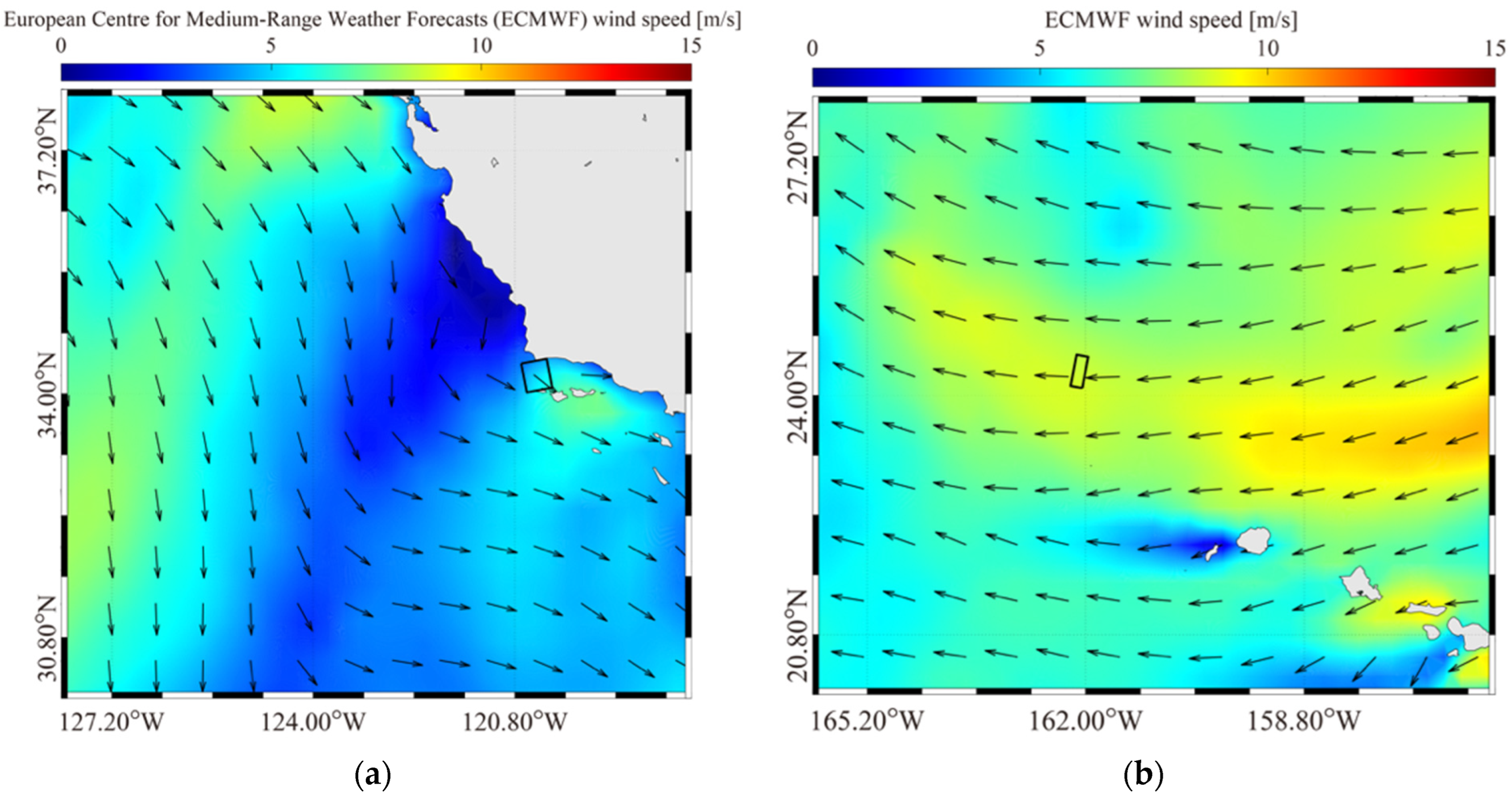
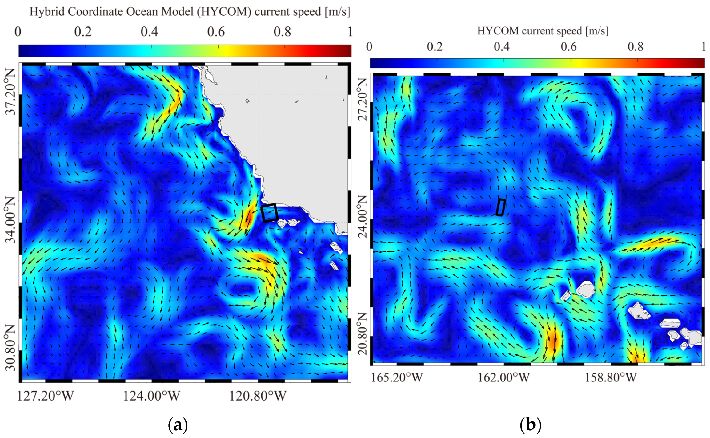
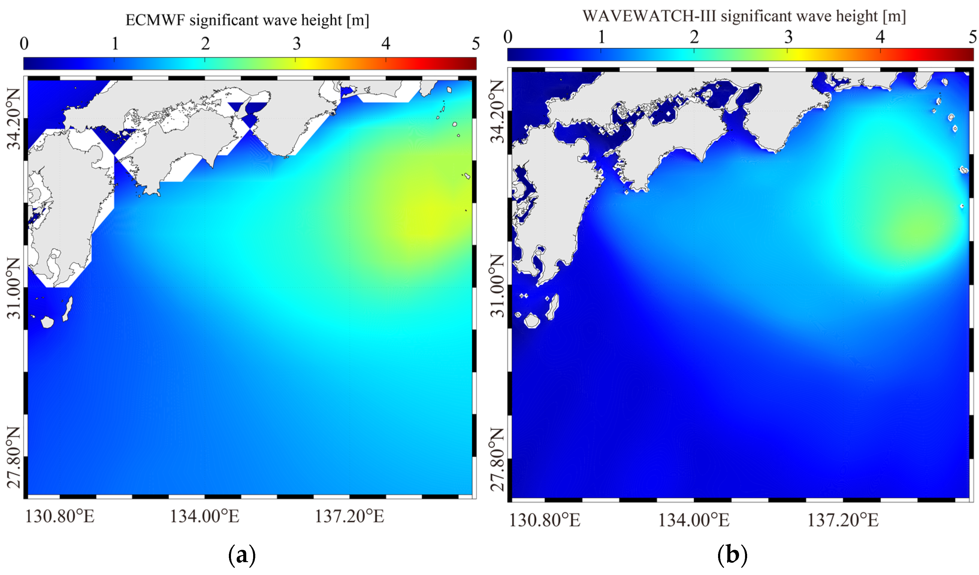
2.2. Hindcast Data
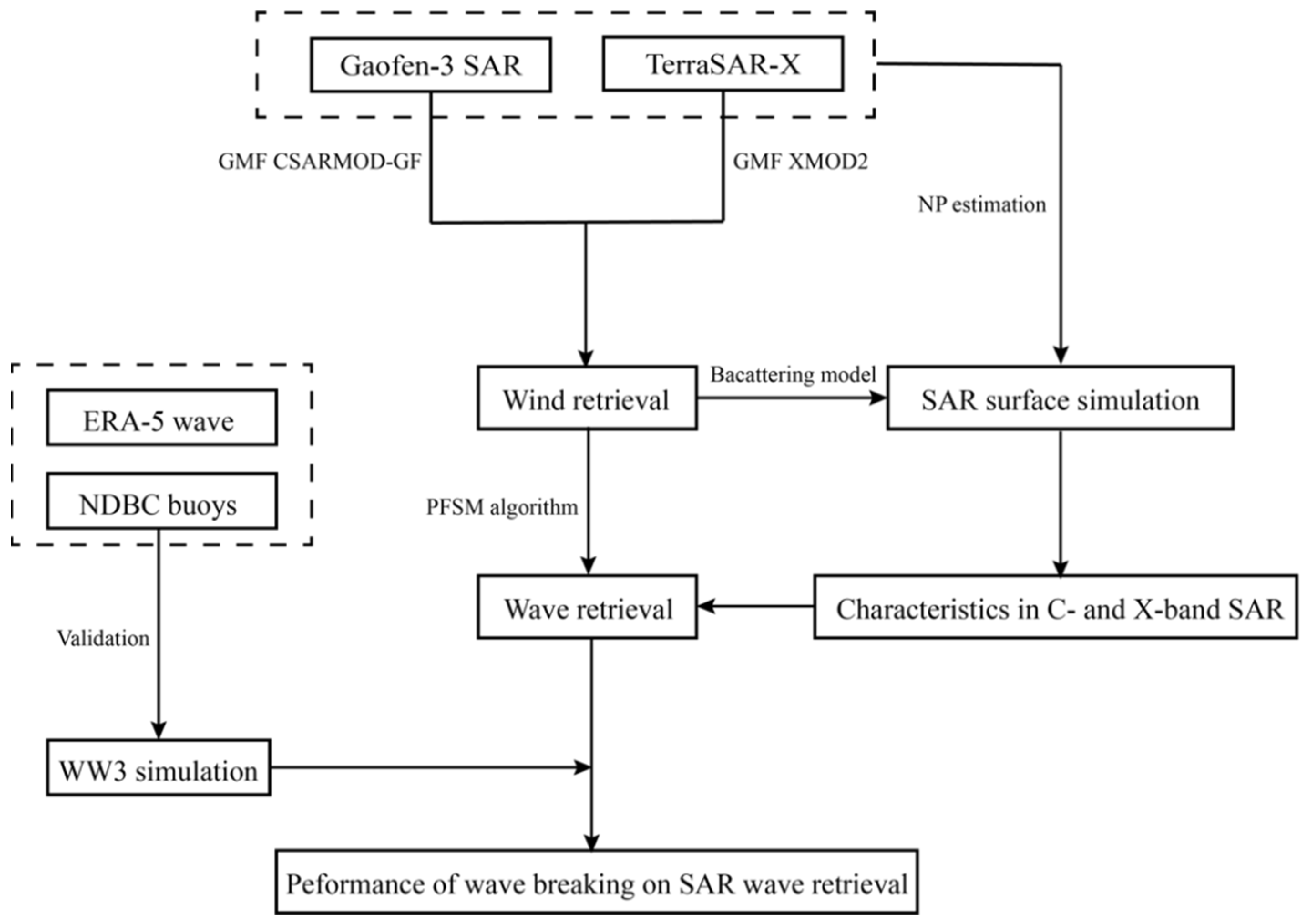
3. Methodology
3.1. NP Estimation
3.2. Radar Backscattering Model
3.3. Wave Retrieval Algorithm
4. Results and Discussion
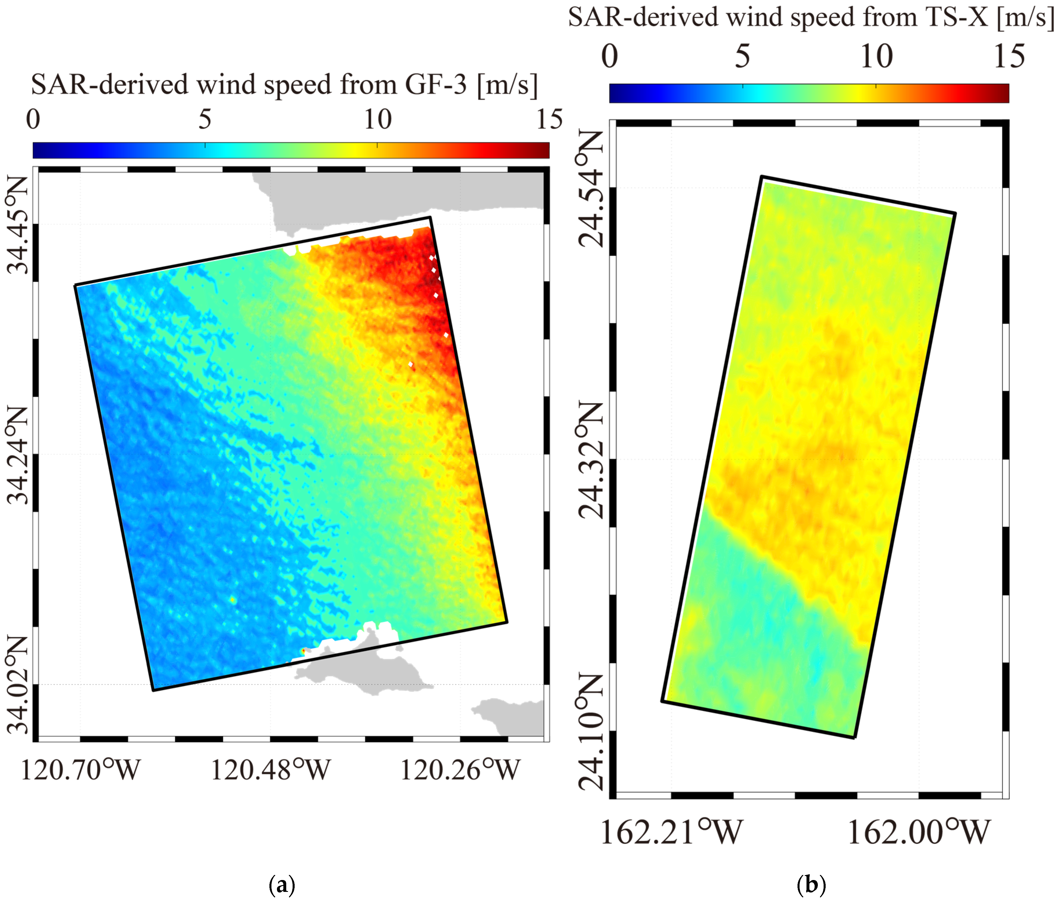
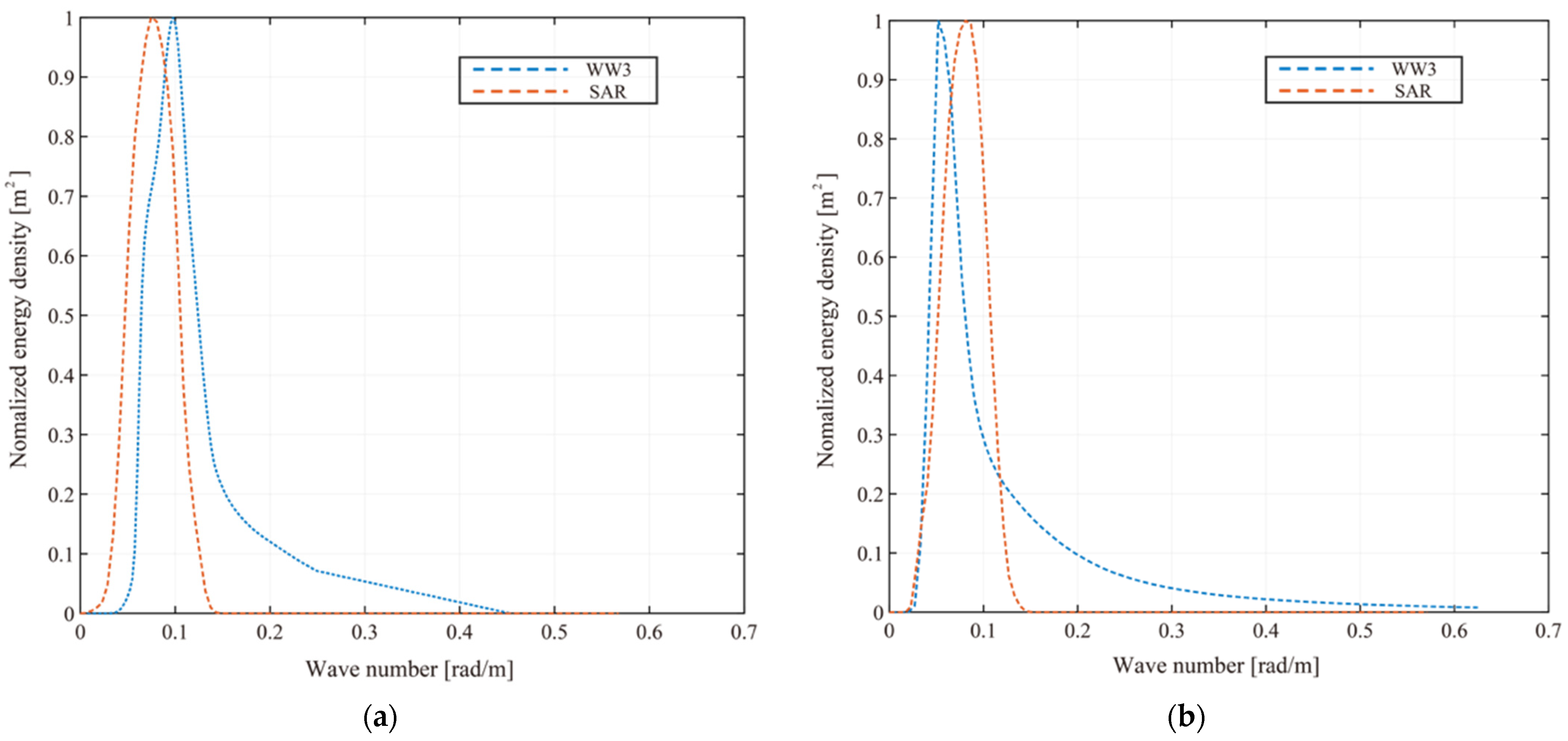
4.1. Wind and Wave Retrieval
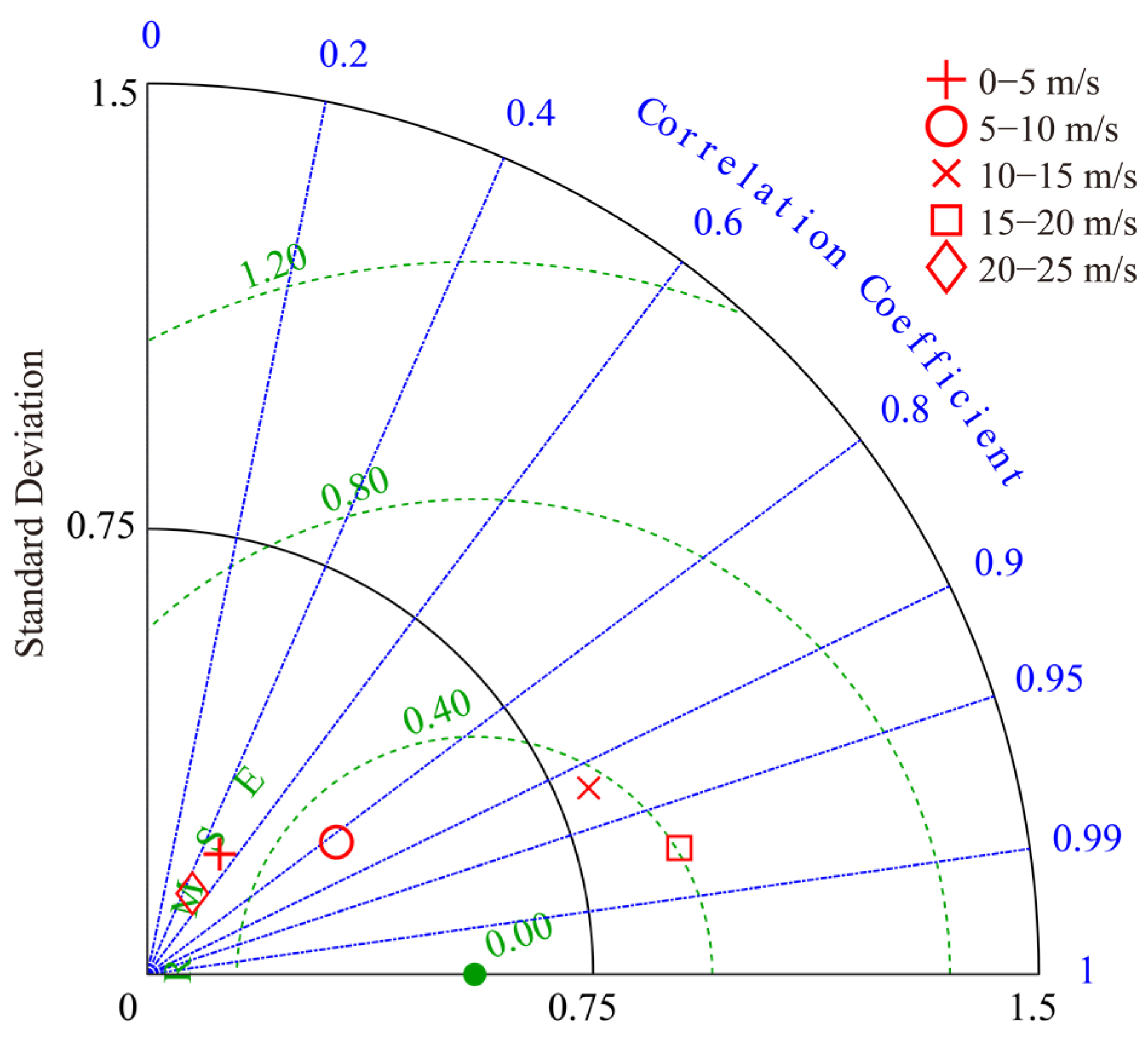
4.2. NP Contribution in Dual-Polarized C-Band and X-Band SAR
4.3. Discussion
5. Conclusions
Author Contributions
Funding
Institutional Review Board Statement
Informed Consent Statement
Data Availability Statement
Acknowledgments
Conflicts of Interest
Appendix A

| Forcing field | European Centre for Medium-Range Weather Forecasts (ECMWF) reanalysis data at a 0.25° gird and a time interval of 1-h sea surface current data from HYbrid Coordinate Ocean Model (HYCOM) at a spatial resolution of 0.08° grid and a time interval of 3-h; and water depth data from the General Bathymetric Chart of the Oceans (GEBCO) having a spatial resolution of 0.01° grid |
| Other settings | The bins ranged logarithmically between 0.04118 and 0.7186 at an interval of Δf/f = 0.1. The spatial propagation was characterized by 300 s time steps in both the longitudinal and latitudinal directions. |
| Resolution | Significant wave height having at a 0.05° gird and temporal resolution of 30-min and the wave spectrum resolved into 24 regular azimuthal directions at a step of 15°. |
| Parameterizations | The input/dissipation terms using switches ST2 and STAB2; the wave-wave interactions using the switch GMD |
Appendix B
References
- Melville, K. The role of surface-wave breaking in air-sea interaction. Annu. Rev. Fluid. Mech. 1996, 28, 279–321. [Google Scholar] [CrossRef]
- Sun, Z.F.; Shao, W.Z.; Yu, W.P.; Li, J. A study of wave-induced effects on sea surface temperature simulations during typhoon events. J. Mar. Sci. Eng. 2021, 9, 622. [Google Scholar] [CrossRef]
- Sun, Z.F.; Shao, W.Z.; Wang, W.L.; Zhou, W.; Yu, W.P.; Shen, W. Analysis of wave-induced stokes transport effects on sea surface temperature simulations in the Western Pacific Ocean. J. Mar. Sci. Eng. 2021, 9, 834. [Google Scholar] [CrossRef]
- Isaksen, L.; Stoffelen, A. ERS scatterometer wind data impact on ECMWF’s tropical cyclone forecasts. IEEE Trans. Geosci. Electron. 2000, 38, 1885–1892. [Google Scholar] [CrossRef]
- Stoffelen, A.; Anderson, T. Wind retrieval and ERS-1 scatterometer radar backscatter measurements. Adv. Space Res. 1993, 13, 53–60. [Google Scholar] [CrossRef]
- Lemoine, F.G.; Zelensky, N.P.; Chinn, D.S.; Pavlis, D.E.; Rowlands, D.D.; Beckley, B.; Luthcke, S.B.; Willis, P.; Ziebart, M.; Luceri, V. Towards development of a consistent orbit series for TOPEX, Jason-1, and Jason-2. Adv. Space. Res. 2010, 46, 1513–1540. [Google Scholar] [CrossRef]
- Hersbach, H. Comparison of C-band scatterometer CMOD5.N equivalent neutral winds with ECMWF. J. Atmos. Ocean. Technol. 2010, 27, 721–736. [Google Scholar] [CrossRef]
- Shao, W.Z.; Nunziata, F.; Zhang, Y.G.; Corcione, V.; Migliaccio, M. Wind speed retrieval from the Gaofen-3 synthetic aperture radar for VV- and HH-polarization using a re-tuned algorithm. Eur. J. Remote Sens. 2021, 54, 318–337. [Google Scholar] [CrossRef]
- Shao, W.Z.; Zhang, Z.; Li, X.M.; Wang, W.L. Sea surface wind speed retrieval from TerraSAR-X HH polarization data using an improved polarization ratio model. IEEE J. Sel. Top. Appl. Earth. Obs. Remote Sens. 2016, 9, 4991–4997. [Google Scholar] [CrossRef]
- Chapron, B.; Johnsen, H.; Garello, R. Wave and wind retrieval from SAR images of the ocean. Ann. Intern. Med. 2001, 56, 682–699. [Google Scholar] [CrossRef]
- Monaldo, M. Comparison of SAR-derived wind speed with model predictions and ocean buoy measurements. IEEE Trans. Geosci. Remote Sens. 2001, 39, 2587–2600. [Google Scholar] [CrossRef]
- Li, X.M.; Lehner, S. Algorithm for sea surface wind retrieval from TerraSAR-X and TanDEM-X data. IEEE Trans. Geosci. Remote Sens. 2014, 52, 2928–2939. [Google Scholar] [CrossRef] [Green Version]
- Shimada, T.; Kawamura, H. An L-band geophysical model function for SAR wind retrieval using JERS-1 SAR. IEEE Trans. Geosci. Remote Sens. 2003, 41, 518–531. [Google Scholar] [CrossRef]
- Yang, X.F.; Li, X.F.; Zheng, Q.A.; Gu, X.F.; Pichel, W.G.; Li, Z.W. Comparison of ocean-surface winds retrieved from QuikSCAT scatterometer and Radarsat-1 SAR in offshore waters of the U.S. west coast. IEEE Geosci. Remote Sens. Lett. 2011, 8, 163–167. [Google Scholar] [CrossRef]
- Yao, R.; Shao, W.Z.; Jiang, X.W.; Yu, T. Wind speed retrieval from Chinese Gaofen-3 synthetic aperture radar using an analytical approach in the nearshore waters of China’s seas. Int. J. Remote Sens. 2022, 43, 3028–3048. [Google Scholar] [CrossRef]
- Shao, W.Z.; Sheng, Y.X.; Sun, J. Preliminary assessment of wind and wave retrieval from Chinese Gaofen-3 SAR imagery. Sensors 2017, 17, 1705. [Google Scholar] [CrossRef] [Green Version]
- Hwang, A.; Zhang, B.; Toporkov, V.; Perrie, W. Comparison of composite Bragg theory and quad-polarization radar backscatter from RADARSAT-2: With applications to wave breaking and high wind retrieval. J. Geophys. Res. Oceans 2010, 115, C08019. [Google Scholar] [CrossRef] [Green Version]
- Zhang, B.; Perrie, W. Cross-Polarized Synthetic Aperture Radar: A new potential measurement technique for hurricanes. Bull. Am. Meteorol. Soc. 2012, 93, 531–541. [Google Scholar] [CrossRef] [Green Version]
- Shao, W.Z.; Yuan, X.Z.; Sheng, Y.X.; Sun, J.; Zhou, W.; Zhang, Q.J. Development of wind speed retrieval from cross-polarization Chinese Gaofen-3 synthetic aperture radar in typhoons. Sensors 2018, 18, 412. [Google Scholar] [CrossRef] [Green Version]
- Engen, G.; Vachon, P.W.; Johnsen, H.; Dobson, F.W. Retrieval of ocean wave spectra and RAR MTF’s from dual-polarization SAR data. IEEE Trans. Geosci. Remote Sens. 2000, 38, 391–403. [Google Scholar] [CrossRef]
- Dankert, H.; Horstmann, J. Detection of wave groups in SAR images and radar image sequences. IEEE Trans. Geosci. Remote Sens. 2003, 41, 1437–1446. [Google Scholar] [CrossRef]
- Alpers, R.; Bruening, C. On the relative importance of motion-related contributions to the SAR Imaging mechanism of ocean surface waves. IEEE Trans. Geosci. Remote Sens. 1986, GE-24, 873–885. [Google Scholar] [CrossRef]
- Alpers, R.; Ross, B.; Rufenach, L. On the detectability of ocean surface waves by real and synthetic aperture radar. J. Geophys. Res. Oceans 1981, 86, 6481. [Google Scholar] [CrossRef]
- Hasselmann, K.; Hasselmann, S. On the nonlinear mapping of an ocean wave spectrum into a synthetic aperture radar image spectrum and its inversion. J. Geophys. Res. Oceans 1991, 96, 10713. [Google Scholar] [CrossRef]
- Mastenbroek, C.; Valk, C. A semiparametric algorithm to retrieve ocean wave spectra from synthetic aperture radar. J. Geophys. Res. Oceans 2000, 105, 3497–3516. [Google Scholar] [CrossRef]
- Schulz-Stellenfleth, J.; Lehner, S.; Hoja, D. A parametric scheme for the retrieval of two-dimensional ocean wave spectra from synthetic aperture radar look cross spectra. J. Geophys. Res. Oceans 2005, 110, C05004. [Google Scholar] [CrossRef] [Green Version]
- Shao, W.Z.; Jiang, X.W.; Sun, Z.F.; Hu, Y.Y.; Marino, A.; Zhang, Y.G. Evaluation of wave retrieval for Chinese Gaofen-3 synthetic aperture radar. Geo-Spat. Inf. Sci. 2022, 25, 229–243. [Google Scholar] [CrossRef]
- Stopa, E.; Mouche, A. Significant wave heights from Sentinel-1 SAR: Validation and applications. J. Geophys. Res. Oceans 2017, 122, 1827–1848. [Google Scholar] [CrossRef] [Green Version]
- Pleskachevsky, L.; Rosenthal, W.; Lehner, S. Meteo-marine parameters for highly variable environment in coastal regions from satellite radar images. ISPRS J. Photogramm. Remote Sens. 2016, 119, 464–484. [Google Scholar] [CrossRef]
- Pleskachevsky, A.; Jacobsen, S.; Tings, B.; Schwarz, E. Estimation of sea state from Sentinel-1 Synthetic aperture radar imagery for maritime situation awareness. Int. J. Remote Sens. 2019, 40, 4104–4142. [Google Scholar] [CrossRef]
- Alpers, W.; Brümmer, B. Atmospheric boundary layer rolls observed by the synthetic aperture radar aboard the ERS-1 satellite. J. Geophys. Res. Oceans 1994, 99, 12613. [Google Scholar] [CrossRef]
- Zhang, L.; Shi, H.; Du, H.; Chen, X. Estimation of sea surface wind direction using spaceborne SAR images and wavelet analysis. J. Remote Sen. 2014, 18, 215–230. [Google Scholar] [CrossRef]
- Kudryavtsev, V.N.; Chapron, B.; Myasoedov, A.G.; Collard, F.; Johannessen, J.A. On dual co-polarized SAR measurements of the ocean surface. IEEE Geosci. Remote Sens. Lett. 2013, 10, 761–765. [Google Scholar] [CrossRef]
- Kudryavtsev, V.; Kozlov, I.; Chapron, B.; Johannessen, J.A. Quad-polarization SAR features of ocean currents. J. Geophys. Res. Oceans 2014, 119, 6046–6065. [Google Scholar] [CrossRef] [Green Version]
- Kudryavtsev, V.; Fan, S.; Zhang, B.; Mouche, A.; Chapron, B. On quad-polarized SAR measurements of the ocean surface. IEEE Trans. Geosci. Remote Sens. 2019, 57, 8362–8370. [Google Scholar] [CrossRef]
- Sun, Z.F.; Shao, W.Z.; Jiang, X.W.; Nunziata, F.; Wang, W.L.; Shen, W.; Migliaccio, M. Contribution of breaking wave on the co-polarized backscattering measured by the Chinese Gaofen-3 SAR. Int. J. Remote Sens. 2022, 43, 1384–1408. [Google Scholar] [CrossRef]
- Viana, R.; Lorenzzetti, J.; Carvalho, J.; Nunziata, F. Estimating energy dissipation rate from breaking waves using polarimetric SAR images. Sensors 2020, 20, 6540. [Google Scholar] [CrossRef]
- Hu, Y.Y.; Shao, W.Z.; Shi, J.; Sun, J.; Ji, Q.Y.; Cai, L.N. Analysis of the typhoon wave distribution simulated in WAVEWATCH- III model in the context of Kuroshio and wind-induced current. J. Oceanol. Limnol. 2020, 38, 1692–1710. [Google Scholar] [CrossRef]
- Plant, J. A stochastic, multiscale model of microwave backscatter from the ocean. J. Geophys. Res. 2002, 107, 3120. [Google Scholar] [CrossRef]
- Xie, T.; Zhao, S.Z.; Perrie, W.; Fang, H.; Yu, W.J.; He, Y.J. Electromagnetic backscattering from one-dimensional drifting fractal sea surface I: Wave–current coupled model. Chin. Phys. B 2016, 25, 064101. [Google Scholar] [CrossRef]
- Kudryavtsev, S.; Hauser, D.; Caudal, G.; Chapron, B. A semiempirical model of the normalized radar cross-section of the sea surface 1. Background model. J. Geophys. Res. 2003, 108, FET21–FET224. [Google Scholar] [CrossRef] [Green Version]
- Phillips, M. Spectral and statistical properties of the equilibrium range in wind-generated gravity waves. J. Fluid. Mech. 1985, 156, 505. [Google Scholar] [CrossRef]
- Pierson, J.; Moskowitz, L. A proposed spectral form for fully developed wind seas based on the similarity theory of S. A. Kitaigorodskii. J. Geophys. Res. Planets 1964, 69, 5181–5190. [Google Scholar] [CrossRef]
- Romeiser, R.; Alpers, W.; Wismann, V. An improved composite surface model for the radar backscattering cross section of the ocean surface: 1. Theory of the model and optimization/validation by scatterometer data. J. Geophys. Res. Oceans 1997, 102, 25237–25250. [Google Scholar] [CrossRef]
- Elfouhaily, T.; Chapron, B.; Katsaros, K.; Vandemark, D. A unified directional spectrum for long and short wind-driven waves. J. Geophys. Res. Oceans 1997, 102, 15781–15796. [Google Scholar] [CrossRef] [Green Version]
- Hasselmann, E.; Dunckel, M.; Ewing, A. Directional wave spectra observed during JONSWAP 1973. J. Phys. Oceanogr. 1980, 10, 1264–1280. [Google Scholar] [CrossRef]
- Shao, W.Z.; Li, X.F.; Sun, J. Ocean wave parameters retrieval from TerraSAR-X images validated against buoy measurements and model results. Remote Sens. 2015, 7, 12815–12828. [Google Scholar] [CrossRef] [Green Version]
- Zhu, S.; Shao, W.Z.; Armando, M.; Shi, J.; Sun, J.; Yuan, X.Z.; Hu, J.C.; Yang, D.K.; Zuo, J.C. Evaluation of Chinese quad-polarization Gaofen-3 SAR wave mode data for significant wave height retrieval. Can. J. Remote Sens. 2019, 44, 588–600. [Google Scholar] [CrossRef]
- Sun, J.; Guan, C.L. Parameterized first-guess spectrum method for retrieving directional spectrum of swell-dominated waves and huge waves from SAR images. Chin. J. Oceanol. Limn. 2006, 24, 12–20. [Google Scholar] [CrossRef]
- Shao, W.; Lai, Z.; Nunziata, F.; Buono, A.; Jiang, X.; Zuo, J. Wind field retrieval with rain correction from dual-polarized Sentinel-1 SAR imagery collected during tropical cyclones. Remote Sens. 2022, 14, 5006. [Google Scholar] [CrossRef]
- Shao, W.; Hu, Y.; Nunziata, F.; Corcione, V.; Migliaccio, M.; Li, X. Cyclone wind retrieval based on X-band SAR-derived wave parameter estimation. J. Atmos. Ocean. Technol. 2020, 37, 1907–1924. [Google Scholar] [CrossRef]
- Zhao, D.L.; Toba, Y. Dependence of whitecap coverage on wind and wind-wave properties. J. Oceanogr. 2001, 57, 603–616. [Google Scholar] [CrossRef]


Disclaimer/Publisher’s Note: The statements, opinions and data contained in all publications are solely those of the individual author(s) and contributor(s) and not of MDPI and/or the editor(s). MDPI and/or the editor(s) disclaim responsibility for any injury to people or property resulting from any ideas, methods, instructions or products referred to in the content. |
© 2023 by the authors. Licensee MDPI, Basel, Switzerland. This article is an open access article distributed under the terms and conditions of the Creative Commons Attribution (CC BY) license (https://creativecommons.org/licenses/by/4.0/).
Share and Cite
Zhong, R.; Shao, W.; Zhao, C.; Jiang, X.; Zuo, J. Analysis of Wave Breaking on Gaofen-3 and TerraSAR-X SAR Image and Its Effect on Wave Retrieval. Remote Sens. 2023, 15, 574. https://doi.org/10.3390/rs15030574
Zhong R, Shao W, Zhao C, Jiang X, Zuo J. Analysis of Wave Breaking on Gaofen-3 and TerraSAR-X SAR Image and Its Effect on Wave Retrieval. Remote Sensing. 2023; 15(3):574. https://doi.org/10.3390/rs15030574
Chicago/Turabian StyleZhong, Ruozhu, Weizeng Shao, Chi Zhao, Xingwei Jiang, and Juncheng Zuo. 2023. "Analysis of Wave Breaking on Gaofen-3 and TerraSAR-X SAR Image and Its Effect on Wave Retrieval" Remote Sensing 15, no. 3: 574. https://doi.org/10.3390/rs15030574