
Quantification of Physiological Parameters of Rice Varieties Based on Multi-Spectral Remote Sensing and Machine Learning Models

Abstract
:1. Introduction
2. Materials and Methods
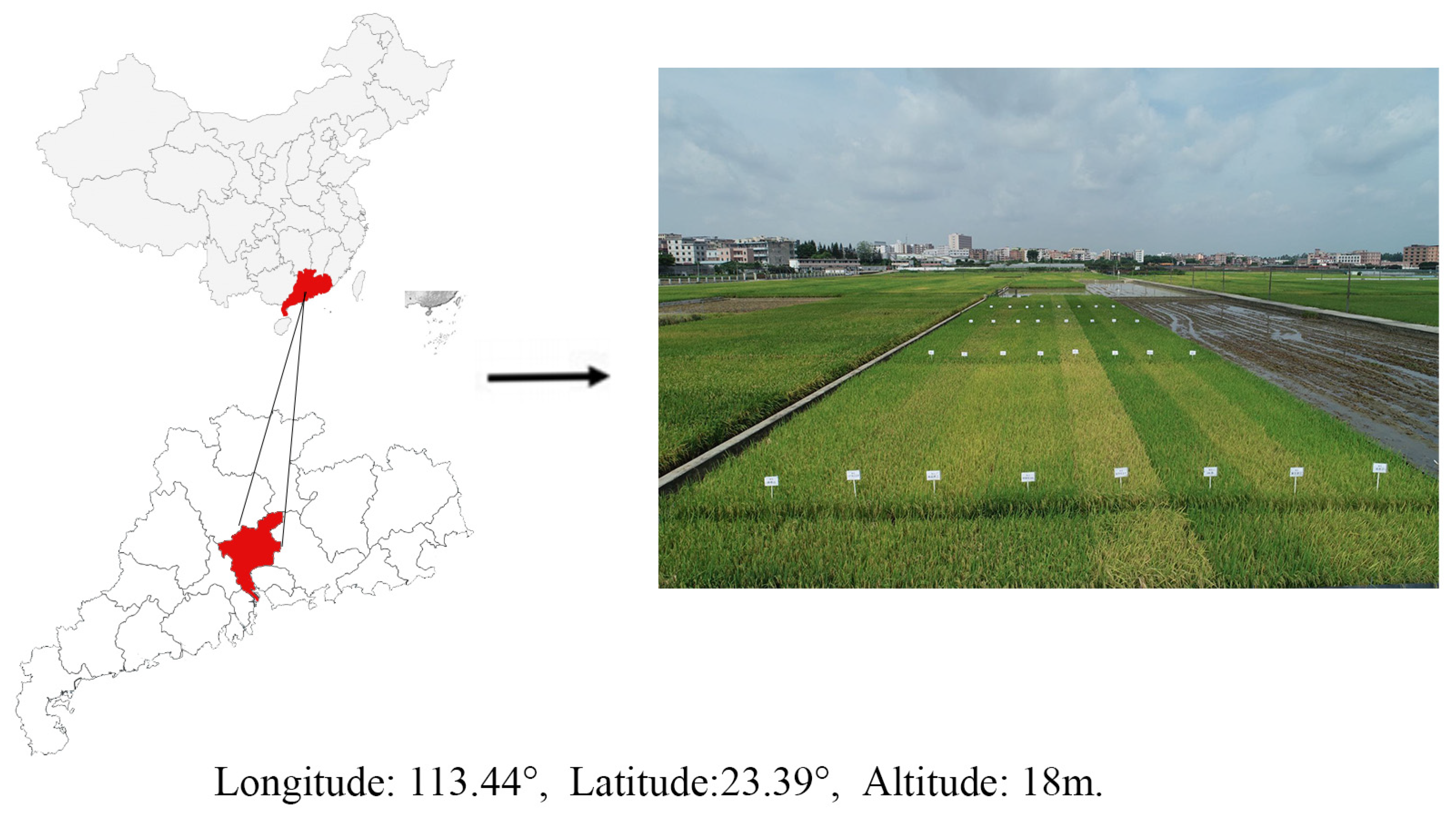
2.1. Experiment Site
2.2. Treatment and Experimental Design
2.3. Ground-Based Field Observations
2.4. The UAV Model
2.5. UAV-Based Field Observations
2.6. Machine Learning Modeling
3. Results
3.1. Rice Biochemical Variation
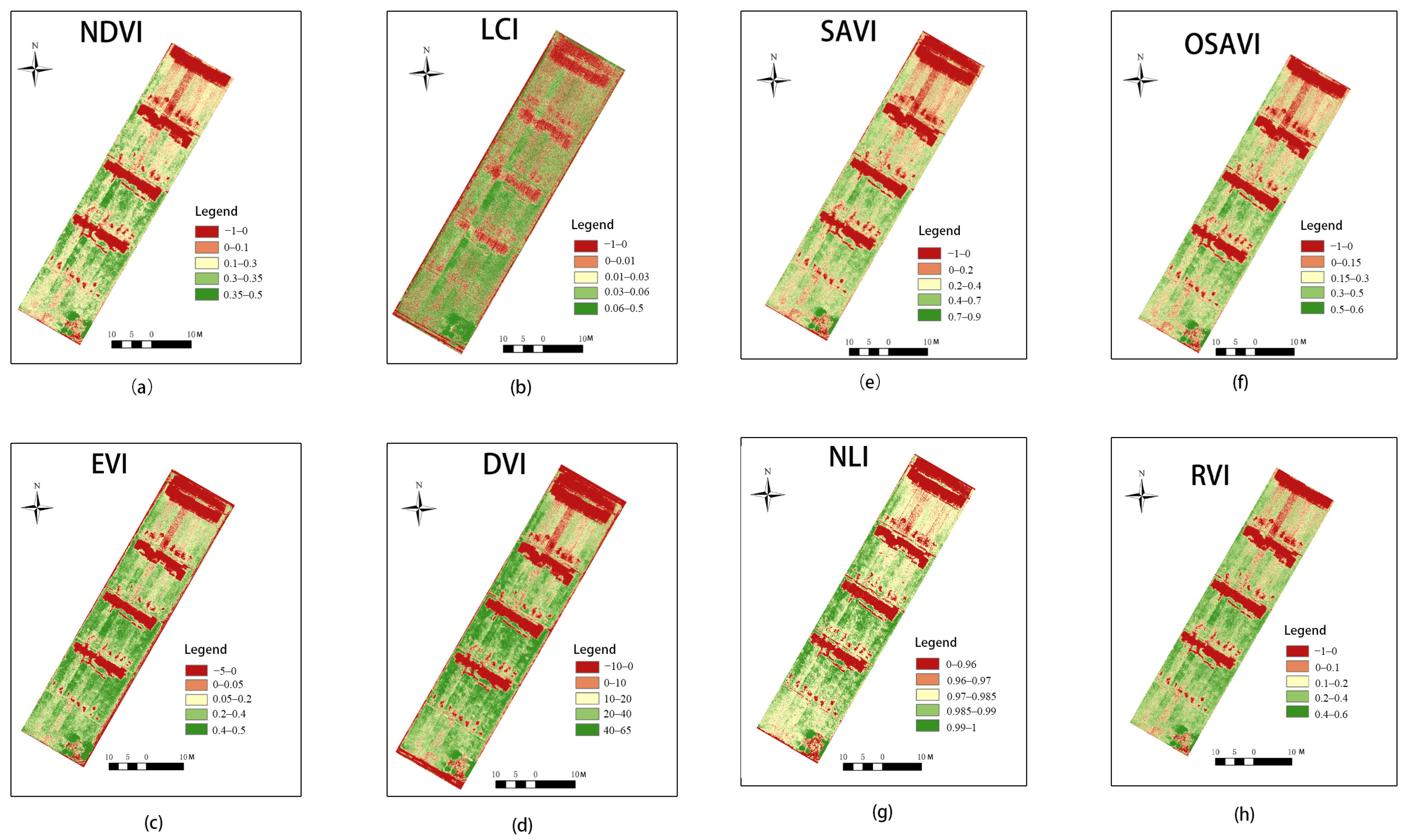
3.2. Change of Rice Vegetation Index
3.3. Single-Factor Regression Modeling
3.4. Analysis of Single-Factor Regression Model Accuracy
3.5. Analysis of Multi-Factor Regression Model Accuracy
4. Discussion
5. Conclusions
- First, the multi-vegetation index composed of nine vegetation indexes was used as the input parameter. Compared with single vegetation, the multi-vegetation index has a better effect in MSE and MAPE. Then, we compared the different machine learning models, and we found that SVM and RF were used to establish the model, and that the overall prediction effect was good, which significantly improved its ability to monitor rice physiological parameters, and effectively reduced its dependence on test conditions such as variety and soil fertility.
- Second, the analysis shows that increasing the amount of nitrogen application can promote rice growth, and increase the chlorophyll concentration, dry matter, and whole leaf area of rice in the early stage of rice growth, but excessive nitrogen application will not even inhibit rice growth.
Author Contributions
Funding
Data Availability Statement
Conflicts of Interest
Appendix A

| Varieties | Reproductive Period | Nitrogen Application Level | SPAD | Dry Matter Weight (kg/666 m2) | Whole Leaf Area (cm2) |
|---|---|---|---|---|---|
| Meixiangzhan 2 | Tillering Stage | N1 | 33.79 ± 0.81 Aa | 239.50 ± 20.10 Abcd | 1105.89 ± 189.30 Aa |
| N2 | 35.97 ± 0.22 Ba | 237.20 ± 9.41 Aa | 1368.00 ± 49.80 Aab | ||
| N3 | 35.98 ± 1.16 Ba | 248.80 ± 17.28 Aab | 1514.91 ± 150.92 Aab | ||
| N4 | 36.50 ± 0.39 Bab | 280.40 ± 31.56 Aabc | 1520.47 ± 169.36 Aa | ||
| Full Heading Stage | N1 | 30.40 ± 0.39 Aa | 628.45 ± 40.35 Aa | 1581.88 ± 79.55 Abc | |
| N2 | 31.35 ± 0.034 Aa | 679.14 ± 28.84 Aab | 1950.26 ± 241.32 Ba | ||
| N3 | 32.77 ± 0.80 Ba | 657.05 ± 41.00 Aa | 2075.52 ± 61.18 BCab | ||
| N4 | 31.33 ± 0.66 Aa | 663.74 ± 49.94 Aa | 2347.00 ± 60.42 Cab | ||
| Ivory Xiangzhan | Tillering Stage | N1 | 36.12 ± 1.26 Ac | 239.30 ± 5.32 Abcd | 1026.09 ± 43.45 Aa |
| N2 | 36.63 ± 1.44 Aab | 259.30 ± 17.77 ABab | 1348.17 ± 132.63 Bab | ||
| N3 | 37.27 ± 0.75 Aa | 287.50 ± 17.49 Bbcd | 1582.71 ± 131.31 Bab | ||
| N4 | 36.37 ± 1.26 Aab | 262.50 ± 12.26 Abab | 1499.07 ± 93.55 Ba | ||
| Full Heading Stage | N1 | 29.53 ± 0.43 Aa | 618.79 ± 69.91 Aa | 1418.39 ± 109.60 Aabc | |
| N2 | 30.33 ± 0.62 Aa | 633.78 ± 32.67 Aab | 1942.61 ± 117.91 Ba | ||
| N3 | 33.47 ± 0.88 Ba | 656.48 ± 44.94 Aa | 1814.85 ± 362.83 ABa | ||
| N4 | 30.93 ± 0.28 Aa | 667.60 ± 39.24 Aa | 1969.68 ± 120.58 Ba | ||
| 19 Xiang | Tillering Stage | N1 | 35.55 ± 0.75 Aabc | 220.60 ± 27.75 Abc | 981.31 ± 156.31 Aa |
| N2 | 36.77 ± 0.79 ABab | 276.30 ± 17.83 Bab | 1261.80 ± 93.41 ABab | ||
| N3 | 37.35 ± 0.73 Ba | 233.30 ± 17.10 ABa | 1290.97 ± 128.16 Ba | ||
| N4 | 37.02 ± 0.11 ABab | 251.00 ± 13.34 ABa | 1304.23 ± 118.67 Ba | ||
| Full Heading Stage | N1 | 35.20 ± 0.63 Ae | 636.16 ± 65.84 Aa | 1345.31 ± 228.15 Aab | |
| N2 | 37.06 ± 0.42 Bd | 736.78 ± 28.50 Abc | 2049.05 ± 67.37 Ba | ||
| N3 | 37.70 ± 0.56 Bc | 681.05 ± 82.11 Aa | 2176.54 ± 232.57 Bab | ||
| N4 | 38.08 ± 0.19 Bd | 819.92 ± 16.708 Bb | 2355.12 ± 286.83 Bab | ||
| Ruanhuayou Jinsi | Tillering Stage | N1 | 34.03 ± 0.77 Aab | 250.30 ± 17.94 Acd | 1079.60 ± 89.80 Aa |
| N2 | 37.17 ± 0.62 Bab | 284.60 ± 30.78 Abb | 1327.44 ± 189.90 Aab | ||
| N3 | 37.57 ± 0.38 Ba | 328.90 ± 38.85 Bd | 1707.20 ± 225.63 Bb | ||
| N4 | 36.89 ± 1.53 Bab | 308.10 ± 9.55 ABc | 1388.70 ± 110.63 ABa | ||
| Full Heading Stage | N1 | 30.93 ± 0.28 Aab | 556.68 ± 17.49 Aa | 1164.75 ± 55.75 Aa | |
| N2 | 32.81 ± 0.88 Bb | 747.33 ± 58.59 Bbc | 2076.61 ± 55.87 Ba | ||
| N3 | 35.31 ± 0.52 Cb | 805.91 ± 36.51 Bb | 2491.95 ± 323.08 Bb | ||
| N4 | 35.62 ± 0.80 Cb | 727.56 ± 30.93 Bab | 2151.58 ± 238.94 Bab | ||
| Qingxiangyou 033 | Tillering Stage | N1 | 35.26 ± 1.14 Aabc | 261.80 ± 13.52 Ad | 1060.26 ± 70.00 Aa |
| N2 | 38.06 ± 0.85 Bab | 283.30 ± 15.31 ABb | 1446.56 ± 84.78 Bb | ||
| N3 | 37.26 ± 0.95 Aba | 324.70 ± 14.64 Cd | 1465.37 ± 51.39 Bab | ||
| N4 | 37.01 ± 1.32 ABab | 302.80 ± 19.94 BCbc | 1421.53 ± 39.42 Ba | ||
| Full Heading Stage | N1 | 31.85 ± 0.85 Abc | 594.13 ± 8.52 Aa | 1762.00 ± 365.02 Ac | |
| N2 | 34.07 ± 0.57 Bbc | 674.58 ± 82.49 (A,ab) | 2128.03 ± 261.29 Aa | ||
| N3 | 33.95 ± 0.84 Ba | 649.02 ± 22.03 (A,a) | 2040.83 ± 272.11 Aab | ||
| N4 | 36.60 ± 0.19 Cbc | 671.64 ± 21.51 (A,a) | 2037.58 ± 89.11 Aa | ||
| Nanjingxiangzhan | Tillering Stage | N1 | 33.90 ± 0.80 Aa | 209.90 ± 17.6155 (A,b) | 1015.77 ± 89.23 Aa |
| N2 | 36.59 ± 1.46 Bab | 241.80 ± 15.35 (AB,ab) | 1203.73 ± 118.34 Aab | ||
| N3 | 36.65 ± 1.32 Ba | 271.50 ± 13.81 (B,abc) | 1438.87 ± 67.69 Bab | ||
| N4 | 35.81 ± 0.32 ABab | 277.50 ± 20.85 (B,abc) | 1473.45 ± 99.02 Ba | ||
| Full Heading Stage | N1 | 32.82 ± 0.65 Acd | 545.54 ± 17.46 (A,a) | 1411.14 ± 112.87 Aabc | |
| N2 | 33.91 ± 0.86 Abc | 704.81 ± 21.53 (B,ab) | 2065.37 ± 217.53 Ba | ||
| N3 | 36.22 ± 0.50 Bb | 658.77 ± 29.27 (AB,a) | 1908.01 ± 128.49 Ba | ||
| N4 | 37.21 ± 0.34 Bcd | 644.48 ± 92.08 (AB,a) | 1992.98 ± 107.71 Ba | ||
| Erguangxiangzhan 3 | Tillering Stage | N1 | 36.73 ± 1.85 Ac | 212.40 ± 15.00 (A,bc) | 991.43 ± 58.72 Aa |
| N2 | 38.33 ± 0.83 Ab | 269.00 ± 13.79 (B,ab) | 1348.92 ± 61.167 Bab | ||
| N3 | 37.31 ± 0.33 Aa | 307.30 ± 9.54 (C,cd) | 1526.36 ± 48.74 Cab | ||
| N4 | 39.25 ± 0.80 Ac | 251.00 ± 18.17 Ba | 1355.34 ± 49.75 Ba | ||
| Full Heading Stage | N1 | 36.25 ± 0.18 Ae | 606.01 ± 45.18 Aa | 1280.40 ± 54.35 Aab | |
| N2 | 38.15 ± 0.74 Bd | 828.62 ± 14.61 ABc | 2206.06 ± 173.17 Ba | ||
| N3 | 39.22 ± 0.55 Bd | 711.63 ± 42.87 ABab | 2068.16 ± 24.20 Bab | ||
| N4 | 41.85 ± 0.88 Ce | 668.51 ± 89.13 Aa | 2001.28 ± 159.28 Ba | ||
| Lixiangzhan 4 | Tillering Stage | N1 | 35.82 ± 0.74 Abc | 233.20 ± 23.89 Aa | 1001.01 ± 72.31 Aa |
| N2 | 36.30 ± 0.40 Aab | 235.00 ± 17.79 Aa | 1187.70 ± 28.84 Ba | ||
| N3 | 36.90 ± 0.10 Aa | 317.20 ± 13.25 Bd | 1530.21 ± 63.41 Cab | ||
| N4 | 38.50 ± 0.65 Bbc | 278.90 ± 15.08 Babc | 1506.64 ± 77.22 Ca | ||
| Full Heading Stage | N1 | 33.62 ± 1.12 Ad | 625.53 ± 13.03 Aa | 1625.80 ± 139.07 Abc | |
| N2 | 34.37 ± 0.56 Ac | 675.57 ± 25.10 Aab | 2125.90 ± 210.50 Aa | ||
| N3 | 35.40 ± 0.21 Ab | 602.42 ± 69.71 Aa | 2176.20 ± 300.37 Bab | ||
| N4 | 35.65 ± 1.07 Ab | 640.96 ± 49.20 Aa | 2513.50 ± 118.29 Bb |
Appendix B
| Vegetation Index | Type | Model Type | MSE | RMSE | MAE | MAPE | SMAPE |
|---|---|---|---|---|---|---|---|
| DVI | SPAD | Linear regression | 4.44 | 2.11 | 1.54 | 4.41 | 4.38 |
| DVI | SPAD | Random tree | 3.29 | 1.81 | 1.35 | 6.60 | 6.54 |
| DVI | SPAD | Random forest | 1.62 | 1.27 | 0.83 | 7.00 | 6.99 |
| DVI | SPAD | SVM | 4.40 | 2.10 | 1.48 | 6.07 | 5.98 |
| EVI | SPAD | Linear regression | 4.20 | 2.05 | 1.50 | 4.30 | 4.29 |
| EVI | SPAD | Random tree | 2.79 | 1.67 | 1.20 | 6.67 | 6.63 |
| EVI | SPAD | Random forest | 0.99 | 1.00 | 0.74 | 7.11 | 7.05 |
| EVI | SPAD | SVM | 3.92 | 1.98 | 1.42 | 6.17 | 6.10 |
| GNDVI | SPAD | Linear regression | 4.79 | 2.19 | 1.61 | 4.61 | 4.59 |
| GNDVI | SPAD | Random tree | 3.61 | 1.90 | 1.25 | 6.49 | 6.42 |
| GNDVI | SPAD | Random forest | 1.04 | 1.02 | 0.72 | 6.91 | 6.86 |
| GNDVI | SPAD | SVM | 4.73 | 2.18 | 1.59 | 6.09 | 6.01 |
| LCI | SPAD | Linear regression | 3.91 | 1.98 | 1.45 | 4.14 | 4.13 |
| LCI | SPAD | Random tree | 2.21 | 1.49 | 1.03 | 6.82 | 6.78 |
| LCI | SPAD | Random forest | 0.68 | 0.82 | 0.57 | 7.31 | 7.25 |
| LCI | SPAD | SVM | 3.25 | 1.80 | 1.28 | 6.36 | 6.31 |
| NDVI | SPAD | Linear regression | 4.10 | 2.02 | 1.48 | 4.22 | 4.21 |
| NDVI | SPAD | Random tree | 2.97 | 1.72 | 1.28 | 6.69 | 6.64 |
| NDVI | SPAD | Random forest | 1.00 | 1.00 | 0.72 | 6.83 | 6.76 |
| NDVI | SPAD | SVM | 3.82 | 1.96 | 1.39 | 6.19 | 6.12 |
| NLI | SPAD | Linear regression | 4.49 | 2.12 | 1.52 | 4.36 | 4.33 |
| NLI | SPAD | Random tree | 3.66 | 1.91 | 1.35 | 6.56 | 6.48 |
| NLI | SPAD | Random forest | 1.31 | 1.14 | 0.75 | 6.82 | 6.76 |
| NLI | SPAD | SVM | 4.52 | 2.13 | 1.52 | 5.98 | 5.88 |
| OSAVI | SPAD | Linear regression | 4.10 | 2.02 | 1.48 | 4.22 | 4.21 |
| OSAVI | SPAD | Random tree | 2.97 | 1.72 | 1.28 | 6.69 | 6.64 |
| OSAVI | SPAD | Random forest | 1.13 | 1.06 | 0.75 | 6.88 | 6.79 |
| OSAVI | SPAD | SVM | 3.82 | 1.96 | 1.39 | 6.19 | 6.12 |
| RVI | SPAD | Linear regression | 4.55 | 2.13 | 1.57 | 4.50 | 4.48 |
| RVI | SPAD | Random tree | 2.97 | 1.72 | 1.28 | 6.69 | 6.64 |
| RVI | SPAD | Random forest | 1.15 | 1.07 | 0.70 | 6.84 | 6.80 |
| RVI | SPAD | SVM | 4.55 | 2.13 | 1.55 | 6.14 | 6.07 |
| SAVI | SPAD | Linear regression | 4.10 | 2.02 | 1.48 | 4.22 | 4.21 |
| SAVI | SPAD | Random tree | 2.97 | 1.72 | 1.28 | 6.69 | 6.64 |
| SAVI | SPAD | Random forest | 1.16 | 1.08 | 0.74 | 7.11 | 7.03 |
| SAVI | SPAD | SVM | 3.83 | 1.96 | 1.39 | 6.19 | 6.12 |
| SIPS2 | SPAD | Linear regression | 5.95 | 2.44 | 1.93 | 5.58 | 5.49 |
| SIPS2 | SPAD | Random tree | 3.64 | 1.91 | 1.29 | 6.36 | 6.30 |
| SIP2 | SPAD | Random forest | 1.49 | 1.22 | 0.79 | 6.55 | 6.46 |
| SIPI2 | SPAD | SVM | 4.79 | 2.19 | 1.60 | 5.80 | 5.67 |
| DVI | Dry matter accumulation | Linear regression | 25,272.66 | 158.97 | 130.24 | 35.04 | 28.83 |
| DVI | Dry matter accumulation | Random tree | 15,235.54 | 123.43 | 81.44 | 56.67 | 46.47 |
| DVI | Dry matter accumulation | Random forest | 6118.24 | 78.22 | 48.79 | 57.85 | 47.21 |
| DVI | Dry matter accumulation | SVM | 40,626.66 | 201.56 | 192.42 | 51.03 | 45.44 |
| EVI | Dry matter accumulation | Linear regression | 12,799.01 | 113.13 | 82.80 | 23.16 | 19.28 |
| EVI | Dry matter accumulation | Random tree | 1718.21 | 41.45 | 27.01 | 59.13 | 48.31 |
| EVI | Dry matter accumulation | Random forest | 669.17 | 25.87 | 16.29 | 59.19 | 48.55 |
| EVI | Dry matter accumulation | SVM | 36,594.71 | 191.30 | 181.56 | 51.02 | 45.42 |
| GNDVI | Dry matter accumulation | Linear regression | 3028.99 | 55.04 | 40.62 | 10.03 | 9.80 |
| GNDVI | Dry matter accumulation | Random tree | 1164.05 | 34.12 | 24.37 | 59.19 | 48.30 |
| GNDVI | Dry matter accumulation | Random forest | 661.81 | 25.73 | 17.81 | 59.43 | 48.54 |
| GNDVI | Dry matter accumulation | SVM | 32,760.81 | 181.00 | 170.95 | 50.66 | 45.40 |
| LCI | Dry matter accumulation | Linear regression | 16,640.53 | 129.00 | 97.03 | 27.92 | 23.57 |
| LCI | Dry matter accumulation | Random tree | 4586.09 | 67.72 | 44.55 | 58.47 | 47.77 |
| LCI | Dry matter accumulation | Random forest | 3798.58 | 61.63 | 34.35 | 58.46 | 47.58 |
| LCI | Dry matter accumulation | SVM | 37,997.51 | 194.93 | 185.09 | 50.98 | 45.43 |
| NDVI | Dry matter accumulation | Linear regression | 11,372.35 | 106.64 | 78.45 | 20.16 | 17.40 |
| NDVI | Dry matter accumulation | Random tree | 1753.56 | 41.88 | 27.49 | 59.16 | 48.34 |
| NDVI | Dry matter accumulation | Random forest | 760.43 | 27.58 | 16.20 | 58.57 | 48.25 |
| NDVI | Dry matter accumulation | SVM | 35,972.30 | 189.66 | 180.11 | 50.98 | 45.42 |
| NLI | Dry matter accumulation | Linear regression | 22,520.33 | 150.07 | 121.80 | 30.74 | 26.16 |
| NLI | Dry matter accumulation | Random tree | 13,801.87 | 117.48 | 69.99 | 56.61 | 46.31 |
| NLI | Dry matter accumulation | Random forest | 6512.88 | 80.70 | 49.70 | 57.12 | 47.02 |
| NLI | Dry matter accumulation | SVM | 39,097.22 | 197.73 | 188.70 | 51.23 | 45.43 |
| OSAVI | Dry matter accumulation | Linear regression | 11,388.91 | 106.72 | 78.52 | 20.18 | 17.41 |
| OSAVI | Dry matter accumulation | Random tree | 1753.56 | 41.88 | 27.49 | 59.16 | 48.34 |
| OSAVI | Dry matter accumulation | Random forest | 558.03 | 23.62 | 15.42 | 59.36 | 48.41 |
| OSAVI | Dry matter accumulation | SVM | 35,978.27 | 189.68 | 180.13 | 50.98 | 45.42 |
| RVI | Dry matter accumulation | Linear regression | 10,965.51 | 104.72 | 72.97 | 22.22 | 19.04 |
| RVI | Dry matter accumulation | Random tree | 1768.99 | 42.06 | 27.07 | 59.12 | 48.30 |
| RVI | Dry matter accumulation | Random forest | 615.61 | 24.81 | 15.74 | 58.77 | 48.37 |
| RVI | Dry matter accumulation | SVM | 35,824.93 | 189.27 | 179.53 | 51.04 | 45.42 |
| SAVI | Dry matter accumulation | Linear regression | 11,423.99 | 106.88 | 78.66 | 20.22 | 17.45 |
| SAVI | Dry matter accumulation | Random tree | 1753.56 | 41.88 | 27.49 | 59.16 | 48.34 |
| SAVI | Dry matter accumulation | Random forest | 557.48 | 23.61 | 15.21 | 59.21 | 48.58 |
| SAVI | Dry matter accumulation | SVM | 35,990.92 | 189.71 | 180.16 | 50.98 | 45.42 |
| SIPS2 | Dry matter accumulation | Linear regression | 39,057.18 | 197.63 | 185.62 | 49.58 | 42.86 |
| SIPS2 | Dry matter accumulation | Random tree | 1409.91 | 37.55 | 28.18 | 59.07 | 48.20 |
| SIP2 | Dry matter accumulation | Random forest | 567.53 | 23.82 | 16.29 | 60.00 | 48.75 |
| SIPI2 | Dry matter accumulation | SVM | 39,490.60 | 198.72 | 189.85 | 50.79 | 45.44 |
| DVI | Whole leaf area | Linear regression | 165,290.47 | 406.56 | 338.79 | 22.50 | 20.84 |
| DVI | Whole leaf area | Random tree | 123,097.42 | 350.85 | 248.08 | 25.74 | 24.21 |
| DVI | Whole leaf area | Random forest | 29,272.65 | 171.09 | 120.38 | 27.75 | 25.88 |
| DVI | Whole leaf area | SVM | 182,313.12 | 426.98 | 347.75 | 21.47 | 21.65 |
| EVI | Whole leaf area | Linear regression | 130,033.38 | 360.60 | 282.98 | 19.21 | 17.43 |
| EVI | Whole leaf area | Random tree | 27,643.13 | 166.26 | 121.24 | 29.65 | 27.95 |
| EVI | Whole leaf area | Random forest | 15,666.32 | 125.17 | 87.33 | 29.67 | 27.82 |
| EVI | Whole leaf area | SVM | 176,291.82 | 419.87 | 342.79 | 21.63 | 21.70 |
| GNDVI | Whole leaf area | Linear regression | 79,538.29 | 282.03 | 220.06 | 14.91 | 13.92 |
| GNDVI | Whole leaf area | Random tree | 17,395.32 | 131.89 | 94.15 | 29.96 | 28.22 |
| GNDVI | Whole leaf area | Random forest | 9462.54 | 97.28 | 64.36 | 30.24 | 28.36 |
| GNDVI | Whole leaf area | SVM | 169,213.80 | 411.36 | 336.42 | 21.73 | 21.73 |
| LCI | Whole leaf area | Linear regression | 134,879.89 | 367.26 | 284.19 | 19.28 | 17.45 |
| LCI | Whole leaf area | Random tree | 71,123.41 | 266.69 | 187.69 | 27.74 | 26.05 |
| LCI | Whole leaf area | Random forest | 28,645.13 | 169.25 | 101.89 | 28.00 | 26.34 |
| LCI | Whole leaf area | SVM | 178,639.35 | 422.66 | 345.00 | 21.59 | 21.69 |
| NDVI | Whole leaf area | Linear regression | 128,002.80 | 357.77 | 280.84 | 18.89 | 17.26 |
| NDVI | Whole leaf area | Random tree | 26,831.71 | 163.80 | 119.40 | 29.71 | 28.01 |
| NDVI | Whole leaf area | Random forest | 12,495.40 | 111.78 | 68.31 | 30.28 | 28.53 |
| NDVI | Whole leaf area | SVM | 174,517.98 | 417.75 | 341.06 | 21.65 | 21.71 |
| NLI | Whole leaf area | Linear regression | 161,138.78 | 401.42 | 329.63 | 21.86 | 20.22 |
| NLI | Whole leaf area | Random tree | 103,305.31 | 321.41 | 210.89 | 26.55 | 24.98 |
| NLI | Whole leaf area | Random forest | 44,411.55 | 210.74 | 126.89 | 27.68 | 25.77 |
| NLI | Whole leaf area | SVM | 178,843.23 | 422.90 | 344.64 | 21.57 | 21.68 |
| OSAVI | Whole leaf area | Linear regression | 128,074.73 | 357.88 | 280.96 | 18.90 | 17.27 |
| OSAVI | Whole leaf area | Random tree | 26,831.71 | 163.80 | 119.40 | 29.71 | 28.01 |
| OSAVI | Whole leaf area | Random forest | 11,681.40 | 108.08 | 70.51 | 29.03 | 27.51 |
| OSAVI | Whole leaf area | SVM | 174,529.22 | 417.77 | 341.07 | 21.65 | 21.71 |
| RVI | Whole leaf area | Linear regression | 113,690.16 | 337.18 | 268.98 | 18.63 | 16.85 |
| RVI | Whole leaf area | Random tree | 26,831.71 | 163.80 | 119.40 | 29.71 | 28.01 |
| RVI | Whole leaf area | Random forest | 11,729.30 | 108.30 | 71.34 | 29.49 | 27.91 |
| RVI | Whole leaf area | SVM | 174,965.33 | 418.29 | 341.81 | 21.65 | 21.71 |
| SAVI | Whole leaf area | Linear regression | 128,226.56 | 358.09 | 281.22 | 18.92 | 17.29 |
| SAVI | Whole leaf area | Random tree | 26,831.71 | 163.80 | 119.40 | 29.71 | 28.01 |
| SAVI | Whole leaf area | Random forest | 7346.30 | 85.71 | 60.75 | 29.92 | 28.27 |
| SAVI | Whole leaf area | SVM | 174,553.00 | 417.80 | 341.08 | 21.65 | 21.71 |
| SIPS2 | Whole leaf area | Linear regression | 153,025.81 | 391.19 | 329.70 | 21.69 | 20.45 |
| SIPS2 | Whole leaf area | Random tree | 34,384.50 | 185.43 | 141.18 | 29.20 | 27.46 |
| SIP2 | Whole leaf area | Random forest | 11,312.49 | 106.36 | 79.31 | 29.11 | 27.41 |
| SIPI2 | Whole leaf area | SVM | 179,197.60 | 423.32 | 344.84 | 21.47 | 21.65 |
References
- Sarma, T.R.; Rai, A.K.; Gupta, S.K.; Vijayan, J.; Devanna, B.N.; Ray, S. Rice blast management through host-plant resistance: Retrospect and prospects. Agric. Res. 2012, 1, 37–52. [Google Scholar] [CrossRef] [Green Version]
- Mourad, R.; Jaafar, H.; Anderson, M.; Gao, F. Assessment of leaf area index models using harmonized land-sat and sentinel-2 surface reflectance data over a semi-arid irrigated landscape. Remote Sens. 2020, 12, 3121. [Google Scholar] [CrossRef]
- Zhao, R.; An, L.; Song, D.; Li, M.; Qiao, L.; Liu, N.; Sun, H. Detection of chlorophyll fluorescence parameters of potato leaves based on continuous wavelet transform and spectral analysis. Spectrochim. Acta A Mol. Biomol. Spectrosc. 2021, 259, 119768. [Google Scholar] [CrossRef]
- Gitelson, A.; Arkebauer, T.; Viña, A.; Skakun, S.; Inoue, Y. Evaluating plant photosynthetic traits via absorption coefficient in the photosynthetically active radiation region. Remote Sens. Environ. 2021, 258, 112401. [Google Scholar] [CrossRef]
- Wu, B.; Zhang, F.; Liu, C.; Zhang, L.; Luo, Z. Comprehensive remote sensing monitoring method for crop growth. J. Remote Sens. 2004, 6, 498–514, (In Chinese with English Abstract). [Google Scholar]
- Wang, D.; Huang, C.; Ma, Q.; Zhao, P.; Zheng, X. Correlation between hyper spectral vegetation index and LAI and above ground fresh biomass of cotton. Xinjiang Agric. Sci. 2008, 5, 787–790, (In Chinese with English Abstract). [Google Scholar]
- Zheng, Y.; Olfert, O.; Brandt, S.; Thomas, g.; Weiss, R.; Sproute, L. Application of hyperspace remote sensing in crop growth monitoring. Meteorol. Environ. Sci. 2007, 1, 10–16, (In Chinese with English Abstract). [Google Scholar]
- Sun, B.; Wang, C.; Yang, C.; Xu, B.; Zhou, G.; Li, X.; Xie, J.; Xu, S.; Liu, B.; Xie, T.; et al. Retrieval of rapeseed leaf area index using the PROSAIL model with canopy coverage derived from UAV images as a correction parameter. Int. J. Appl. Earth Obs. Geoinf. 2021, 102, 102373. [Google Scholar] [CrossRef]
- Gidudu, A.; Letaru, L.; Kulabako, R.N. Empirical modeling of chlorophyll a from MODIS satellite imagery for trophic status monitoring of lake Victoria in east Africa. J. Great Lakes Res. 2021, 47, 1209–1218. [Google Scholar] [CrossRef]
- Martinez, K.P.; Burgos, D.F.M.; Blanco, A.C.; Salmo, S.G. Multi-sensor approach to leaf area index estimation using statistical machine learning models: A case on mangrove forests. ISPRS Ann. Photogramm. Remote Sens. Spat. Inf. Sci. 2021, V-3-2021, 109–115. [Google Scholar] [CrossRef]
- Gupta, S.D.; Ibaraki, Y.; Pattanayak, A.K. Development of a digital image analysis method for real-time estimation of chlorophyll content in micropropagated potato plants. Plant Biotechnol. Rep. 2012, 7, 91–97. [Google Scholar] [CrossRef]
- Zheng, H.-L.; Liu, Y.-C.; Qin, Y.-L.; Chen, Y.; Fan, M.-S. Establishing dynamic thresholds for potato nitrogen status diagnosis with the SPAD chlorophyll meter. J. Integr. Agric. 2015, 14, 190–195. [Google Scholar] [CrossRef]
- Rigon, J.P.G.; Capuani, S.; Fernandes, D.M.; Guimarães, T.M. A novel method for the estimation of soybean chlorophyll content using a smartphone and image analysis. Photosynthetica 2016, 54, 559–566. [Google Scholar] [CrossRef]
- Qi, H.; Wu, Z.; Zhang, L.; Li, J.; Zhou, J.; Jun, Z.; Zhu, B. Monitoring of peanut leaves chlorophyll content based on drone-based multi-spectral image feature extraction. Comput. Electron. Agric. 2021, 187, 106292. [Google Scholar] [CrossRef]
- Oliveira, R.A.; Junior, J.M.; Costa, C.S.; Näsi, R.; Koivumäki, N.; Niemeläinen, O.; Kaivosoja, J.; Nyholm, L.; Pistori, H.; Honkavaara, E. Silage grass sward nitrogen concentration and dry matter yield estimation using deep regression and RGB Images Captured by UAV. Agronomy 2022, 12, 1352. [Google Scholar] [CrossRef]
- Olfs, H.-W.; Blankenau, K.; Brentrup, F.; Jasper, J.; Link, A.; Lammel, J. Soil- and plant-based nitrogen-fertilizer recommendations in arable farming. J. Plant Nutr. Soil Sci. 2005, 168, 414–431. [Google Scholar] [CrossRef]
- Li, F.; Mistele, B.; Hu, Y.; Chen, X.; Schmidhalter, U. Reflectance estimation of canopy nitrogen content in winter wheat using optimised hyperspectral spectral indices and partial least squares regression. Eur. J. Agron. 2014, 52, 198–209. [Google Scholar] [CrossRef]
- Lilienthal, H. Optical sensors in agriculture: Principles and concepts. J. Für Kult. 2014, 66, 34–41. [Google Scholar] [CrossRef]
- Heinemann, P.; Haug, S.; Schmidhalter, U. Evaluating and defining agronomically relevant detection limits for spectral reflectance-based assessment of N uptake in wheat. Eur. J. Agron. 2022, 140, 126609. [Google Scholar] [CrossRef]
- Tsuchikawa, S.; Ma, T.; Inagaki, T. Application of near-infrared spectroscopy to agriculture and forestry. Anal. Sci. 2022, 38, 635–642. [Google Scholar] [CrossRef]
- Lan, Y.; Thomson, S.J.; Huang, Y.; Hoffmann, W.C.; Zhang, H. Current status and future directions of precision aerial application for site-specific crop management in the USA. Comput. Electron. Agric. 2010, 74, 34–38. [Google Scholar] [CrossRef] [Green Version]
- Niu, Y.; Han, W.; Zhang, H.; Zhang, L.; Chen, H. Estimating fractional vegetation cover of maize under water stress from UAV multispectral imagery using machine learning algorithms. Comput. Electron. Agric. 2021, 189, 106414. [Google Scholar] [CrossRef]
- Yang, K.; Gong, Y.; Fang, S.; Duan, B.; Yuan, N.; Peng, Y.; Wu, X.; Zhu, R. Combining spectral and texture features of UAV images for the remote estimation of rice LAI throughout the entire growing season. Remote Sens. 2021, 13, 3001. [Google Scholar] [CrossRef]
- Liu, L. Unmanned remote sensing imagery-based inversion of major cotton growth parameters. Shandong Norm. Univ. 2019, 9, 1–70, (In Chinese with English Abstract). [Google Scholar]
- Carmonaet, F.; Rivas, R.; Fonnegra, D.C. Vegetation Index to estimate chlorophyll content from multispectral remote sensing data. Eur. J. Remote Sens. 2015, 48, 319–326. [Google Scholar] [CrossRef] [Green Version]
- Zhao, D.; Reddy, K.R.; Kakani, V.G.; Read, J.J.; Koti, S. Canopy Reflectance in Cotton for Growth Assessment and Lint Yield Prediction. Eur. J. Agron. 2007, 26, 335–344. [Google Scholar] [CrossRef]
- Lefsky, M.A.; Cohen, W.B.; Spies, T.A. An evaluation of alternate remote sensing products for forest inventory, monitoring, and mapping of Douglas-fir forests in western Oregon. Can. J. For. Res. 2001, 31, 78–87. [Google Scholar] [CrossRef]
- Jordan, M.I.; Mitchell, T.M. Machine learning: Trends, perspectives, and prospects. Science 2015, 349, 255–260. [Google Scholar] [CrossRef]
- Shao, G.M.; Han, W.T.; Zhang, H.H.; Zhang, L.Y.; Wang, Y.; Zhang, Y. Prediction of maize crop coefficient from UAV multisensor remote sensing using machine learning methods. Agric. Water Manag. 2023, 276, 108064. [Google Scholar] [CrossRef]
- Sun, S.L.; Cao, Z.H.; Zhu, H.; Zhao, J. A Survey of Optimization Methods from a Machine Learning Perspective. IEEE Trans. Cybern. 2020, 50, 3668–3681. [Google Scholar] [CrossRef] [Green Version]
- Chen, L.; Ren, C.; Zhang, B.; Wang, Z.; Xi, Y. Estimation of forest above-ground biomass by geographically weighted regression and machine learning with sentinel imagery. Forests 2018, 9, 582. [Google Scholar] [CrossRef] [Green Version]
- Ghosh, S.M.; Behera, M.D. Aboveground biomass estimation using multi-sensor data synergy and machine learning algorithms in a dense tropical forest. Appl. Geogr. 2018, 96, 29–40. [Google Scholar] [CrossRef]
- Yadav, S.; Padalia, H.; Sinha, S.K.; Srinet, R.; Chauhan, P. Above-ground biomass estimation of Indian tropical forests using X band Pol-InSAR and Random Forest. Remote Sens. Appl. Soc. Environ. 2021, 21, 100462. [Google Scholar] [CrossRef]
- Wu, C.; Shen, H.; Shen, A.; Deng, J.; Gan, M.; Zhu, J.; Xu, H.; Wang, K. Comparison of machine-learning methods for above-ground biomass estimation based on Landsat imagery. J. Appl. Remote Sens. 2016, 10, 035010. [Google Scholar] [CrossRef]
- Hu., L.; Qing., T. Nitrogen use efficiency and research progress of rice in China. Crop Res. 2006, 16, 401–404, (In Chinese with English Abstract). [Google Scholar]
- Wu, Y.; Xu, Y.; Xing, S.; Ma, F.; Chen, N.; Ma, Y. Effects of biochar on transformation and loss of nitrogen and phosphorus in soil. J. Agric. 2018, 9, 20–26, (In Chinese with English Abstract). [Google Scholar]
- Jordan, C.F. Derivation of leaf-area index from quality of light on the forest floor. Ecology 1969, 50, 663–666. [Google Scholar] [CrossRef]
- Tucker, C.J. Red and photographic infrared linear combinations for monitoring vegetation. Remote Sens. Environ. 1979, 8, 127–150. [Google Scholar] [CrossRef] [Green Version]
- Liu, H.Q.; Huete, A. Feedback based modification of the NDVI to minimize canopy background feedback-based noise. IEEE Trans. Geosci. Remote Sens. 1995, 33, 457–465. [Google Scholar] [CrossRef]
- Gitelson, A.A.; Kaufman, Y.J.; Merzlyak, M.N. Use of a green channel in remote sensing of global vegetation from EOS-MODIS. Remote Sens. Environ. 1996, 58, 289–298. [Google Scholar] [CrossRef]
- Goel, N.S.; Qin, W. Influences of canopy architecture on relationships between various vegetation indices and LAI and Fpar: A computer simulation. Remote Sens. Rev. 1994, 10, 309–347. [Google Scholar] [CrossRef]
- Huete, A.R. A soil-adjusted vegetation index (SAVI). Remote Sens. Environ. 1988, 25, 295–309. [Google Scholar] [CrossRef]
- Rondeaux, G.; Steven, M.; Baret, F. Optimization of soil-adjusted vegetation indices. Remote Sens Environ. 1996, 55, 95–107. [Google Scholar] [CrossRef]
- Su, W.; Yang, Y.; Yang, G. Study on the distribution characteristics of thermal field and its relationship with land use/cover in nanjing. Geogr. Sci. 2005, 6, 6697–6703, (In Chinese with English Abstract). [Google Scholar]
- Xu, Y.; Liu, W.; Huo, J.; Liu, J.; Li, H.; Nuerlan, M. Estimation model of chlorophyll content of artemisia annua based on spectral index. People’s Pearl River 2018, 39, 83–91, (In Chinese with English Abstract). [Google Scholar]
- Shi, Z.; Gao, S.; Li, T.; Li, Y.; Li, H.; Liao, Y. Effects of nitrogen application rate on growth, yield and quality of wheat with different chlorophyll content. J. Wheat Crops 2021, 41, 1134–1142, (In Chinese with English Abstract). [Google Scholar]
- Liao, D.; Yun, T.; Liu, Z.; Wu, Z.; Huang, X.; Chen, Y.; Xie, D. Effects of grafting and nitrogen application on dry matter, nitrogen accumulation and nitrogen metabolism enzymes of winter melon. J. Trop. Crops. 2022, 43, 1–11, (In Chinese with English Abstract). [Google Scholar]
- Li, F.; Kong, Q.; Zhang, Q. Estimation of chlorophyll content in guanxi honey pomelo leaves based on spectral characteristic parameters. Fujian Agric. J. 2021, 36, 1447–1456, (In Chinese with English Abstract). [Google Scholar]
- Sun, T.; Yang, X.; Tan, X.; Han, K.; Tang, S.; Tong, W.; Zhu, S.; Hu, Z.; Wu, L. Comparison of agronomic performance between japonica/indica hybrid and japonica cultivars of rice based on different nitrogen rates. Agronomy 2020, 10, 171. [Google Scholar] [CrossRef] [Green Version]
- Rajesh, K.; Ramesh, T. Influence of nitrogen levels on physiological response, nitrogen use efficiency and yield of rice (Oryza sativa L.) genotypes. JAST 2020, 42, 145–152. [Google Scholar] [CrossRef]
- Liu, Y.; Liu, H.; Wang, L.; Xu, M.; Cohen, S.; Liu, K. Derivation of spatially detailed lentic habitat map and inventory at a basin scale by integrating multi-spectral sentinel-2 satellite imagery and USGS digital elevation models. J. Hydrol. 2021, 603, 126876. [Google Scholar] [CrossRef]
- Guo, Y.; Wang, H.; Wu, Z.; Wang, S.; Sun, H.; Senthilnath, J.; Wang, J.; Bryant, C.R.; Fu, Y. Modified red blue vegetation index for chlorophyll estimation and yield prediction of maize from visible images captured by UAV. Sensors 2020, 20, 5055. [Google Scholar] [CrossRef] [PubMed]
- Zhang, H.; Bauters, M.; Boeckx, P.; Oost, K.V. Mapping canopy heights in dense tropical forests using low-cost UAV-derived photographic point clouds and machine learning approaches. Remote Sens. 2021, 13, 3777. [Google Scholar] [CrossRef]
- Kim, D.-K.; Kim, Y.; Kim, K.-H.; Kim, H.-J.; Chung, Y.S. Case study: Cost-effective weed patch detection by multi-spectral camera mounted on unmanned aerial vehicle in the buckwheat field. Korean J. Crop Sci. 2019, 64, 159–164. [Google Scholar] [CrossRef]
- He, G.; Wu, J.; Peng, J.; Gu, S. Estimation model of chlorophyll content in heather leaves based on hyper-spectral. J. Northwest For. Univ. 2022, 1, 1–9, (In Chinese with English Abstract). [Google Scholar]


| Type | Number of Samples | Max | Min | Average | Standard Deviation |
|---|---|---|---|---|---|
| SPAD value | 64 | 41.85 | 29.52 | 35.54 | 2.61 |
| Dry matter accumulation (kg/666 m2) | 64 | 828.61 | 209.94 | 467.24 | 210.86 |
| Whole leaf area (cm2) | 64 | 2513.47 | 981.31 | 1633.36 | 428.17 |
| Band | Central Wavelength (nm) | Width (nm) |
|---|---|---|
| Edge | 730 | 32 |
| Near-infrared | 840 | 52 |
| Green | 560 | 32 |
| Red | 650 | 32 |
| Blue | 450 | 32 |
| Vegetation Index | Formula | Reference |
|---|---|---|
| RVI | Rnir/R | Jordan (1969) [37] |
| NDVI | (RNIR-R)/(RNIR + R) | Tucker (1979) [38] |
| EVI | 2.5 ×(NIR-R)/(NIR + 6 R − 7.5 B + 1) | Hui et al. (1995) [39] |
| GNDVI | (NIR-G)/(NIR + G) | Anatoly et al. (1996) [40] |
| NLI | (NIR × NIR-R)/(NIR× NIR + R) | Goel et al. (1994) [41] |
| SAVI | (1 + 0.5)× (NIR-R)/(NIR + R + 0.5) | Huete (1988) [42] |
| OSAVI | (1 + 0.16)× (NIR-R)/(NIR + R + 0.16) | Geneviève et al. (1996) [43] |
| LCI | (NIR-RedEdge)/(NIR + RedEdge) | Su et al. (2005) [44] |
| SIPI2 | (NIR-Green)/(NIR − Red) | Yue et al. (2018) [45] |
| Type (R2) | Vegetation Index | Linear Regression Model | Random Tree Model | Random Forest Model | SVM |
|---|---|---|---|---|---|
| SPAD Value | EVI | 0.45 | 0.02 | 0.26 | 0.41 |
| GNDVI | 0.33 | 0.33 | 0.07 | 0.29 | |
| LCI | 0.47 | 0.11 | 0.61 | 0.57 | |
| NDVI | 0.53 | −0.30 | 0.09 | 0.32 | |
| NLI | 0.21 | 0.15 | 0.04 | 0.31 | |
| OSAVI | 0.33 | 0.49 | 0.62 | 0.50 | |
| RVI | 0.26 | 0.15 | −0.09 | 0.23 | |
| SAVI | 0.40 | 0.18 | 0.23 | 0.26 | |
| SIPI2 | 0.26 | −0.13 | −0.24 | 0.19 | |
| Dry matter | EVI | 0.83 | 0.92 | 0.95 | 0.11 |
| accumulation | GNDVI | 0.97 | 0.97 | 0.94 | 0.84 |
| LCI | 0.73 | 0.46 | 0.69 | 0.36 | |
| NDVI | 0.89 | 0.96 | 0.92 | 0.92 | |
| NLI | 0.70 | 0.81 | 0.83 | 0.31 | |
| OSAVI | 0.82 | 0.80 | 0.96 | 0.87 | |
| RVI | 0.84 | 0.98 | 0.98 | 0.92 | |
| SAVI | 0.78 | 0.94 | 0.97 | 0.88 | |
| SIPI2 | 0.10 | 0.94 | 0.94 | 0.87 | |
| Whole leaf area | EVI | 0.29 | 0.72 | 0.87 | 0.00 |
| GNDVI | 0.70 | 0.38 | 0.36 | 0.02 | |
| LCI | 0.36 | 0.36 | 0.06 | 0.05 | |
| NDVI | 0.39 | 0.71 | 0.05 | 0.03 | |
| NLI | 0.05 | 0.05 | 0.36 | 0.02 | |
| OSAVI | 0.45 | 0.73 | 0.71 | 0.49 | |
| RVI | 0.36 | 0.40 | 0.41 | 0.02 | |
| SAVI | 0.59 | 0.45 | 0.83 | 0.83 | |
| SIPI2 | 0.23 | 0.40 | 0.56 | 0.34 |
| Type (MAPE) | Vegetation Index | Linear Regression Model | Random Tree Model | Random Forest Model | SVM |
|---|---|---|---|---|---|
| SPAD | EVI | 4.30 | 6.53 | 7.06 | 6.02 |
| GNDVI | 3.75 | 6.38 | 6.23 | 4.35 | |
| LCI | 2.98 | 6.55 | 7.16 | 6.64 | |
| NDVI | 3.55 | 5.60 | 5.82 | 6.17 | |
| NLI | 3.30 | 7.21 | 5.81 | 4.82 | |
| SAVI | 3.21 | 6.97 | 5.53 | 5.54 | |
| RVI | 3.82 | 6.26 | 7.92 | 5.04 | |
| SAVI | 3.94 | 7.82 | 6.02 | 6.15 | |
| SIPI2 | 5.20 | 6.37 | 5.64 | 5.34 | |
| Dry matter | EVI | 16.38 | 43.42 | 56.49 | 68.53 |
| accumulation | GNDVI | 9.75 | 54.36 | 55.79 | 36.28 |
| LCI | 23.31 | 62.17 | 62.20 | 49.32 | |
| NDVI | 11.33 | 58.03 | 58.59 | 72.96 | |
| NLI | 24.19 | 59.36 | 53.32 | 55.54 | |
| SAVI | 13.75 | 53.95 | 54.76 | 43.04 | |
| RVI | 17.20 | 61.59 | 56.17 | 90.88 | |
| SAVI | 19.92 | 53.53 | 60.65 | 53.52 | |
| SIPI2 | 49.22 | 60.62 | 60.11 | 46.40 | |
| Whole leaf area | EVI | 19.77 | 26.36 | 30.23 | 22.66 |
| GNDVI | 13.12 | 37.82 | 36.00 | 19.16 | |
| LCI | 13.52 | 27.81 | 23.02 | 16.47 | |
| NDVI | 12.97 | 24.94 | 31.77 | 18.66 | |
| NLI | 16.76 | 27.89 | 25.38 | 17.84 | |
| SAVI | 12.01 | 28.91 | 25.19 | 19.71 | |
| RVI | 14.90 | 30.68 | 32.76 | 20.04 | |
| SAVI | 10.71 | 21.95 | 28.99 | 24.60 | |
| SIPI2 | 20.97 | 28.69 | 22.24 | 21.94 |
| Type | Model Type | RMSE | MAE | MAPE | SMAPE |
|---|---|---|---|---|---|
| SPAD value | Linear regression | 1.71 | 0.17 | 1.38 | 3.80 |
| Random tree | 1.91 | 1.46 | 10.70 | 10.82 | |
| Random forest | 1.49 | 0.55 | 1.18 | 7.30 | |
| SVM | 1.38 | 0.13 | 0.86 | 4.13 | |
| Dry matter accumulation | Linear model | 59.11 | 55.33 | 15.13 | 14.01 |
| Random tree | 210.85 | 126.58 | 48.02 | 37.31 | |
| Random forest | 24.27 | 17.17 | 60.58 | 49.54 | |
| SVM | 201.25 | 182.80 | 61.96 | 44.79 | |
| Whole leaf area | Linear regression | 363.39 | 315.38 | 25.46 | 21.76 |
| Random tree | 146.26 | 108.63 | 24.80 | 23.96 | |
| Random forest | 201.89 | 161.34 | 27.07 | 26.76 | |
| SVM | 371.36 | 326.82 | 24.68 | 22.72 |
Disclaimer/Publisher’s Note: The statements, opinions and data contained in all publications are solely those of the individual author(s) and contributor(s) and not of MDPI and/or the editor(s). MDPI and/or the editor(s) disclaim responsibility for any injury to people or property resulting from any ideas, methods, instructions or products referred to in the content. |
© 2023 by the authors. Licensee MDPI, Basel, Switzerland. This article is an open access article distributed under the terms and conditions of the Creative Commons Attribution (CC BY) license (https://creativecommons.org/licenses/by/4.0/).
Share and Cite
Liu, S.; Zhang, B.; Yang, W.; Chen, T.; Zhang, H.; Lin, Y.; Tan, J.; Li, X.; Gao, Y.; Yao, S.; et al. Quantification of Physiological Parameters of Rice Varieties Based on Multi-Spectral Remote Sensing and Machine Learning Models. Remote Sens. 2023, 15, 453. https://doi.org/10.3390/rs15020453
Liu S, Zhang B, Yang W, Chen T, Zhang H, Lin Y, Tan J, Li X, Gao Y, Yao S, et al. Quantification of Physiological Parameters of Rice Varieties Based on Multi-Spectral Remote Sensing and Machine Learning Models. Remote Sensing. 2023; 15(2):453. https://doi.org/10.3390/rs15020453
Chicago/Turabian StyleLiu, Shiyuan, Bin Zhang, Weiguang Yang, Tingting Chen, Hui Zhang, Yongda Lin, Jiangtao Tan, Xi Li, Yu Gao, Suzhe Yao, and et al. 2023. "Quantification of Physiological Parameters of Rice Varieties Based on Multi-Spectral Remote Sensing and Machine Learning Models" Remote Sensing 15, no. 2: 453. https://doi.org/10.3390/rs15020453