Remote Sensing in Field Crop Monitoring: A Comprehensive Review of Sensor Systems, Data Analyses and Recent Advances

Abstract

The key elements that underpin food security require the adaptation of agricultural systems to support productivity increases while minimizing inputs and the adverse effects of climate change. The advances in precision agriculture over the past few years have substantially enhanced the efficiency of applying spatially variable agronomic inputs for irrigation, such as fertilizers, pesticides, seeds, and water, and we can attribute them to the increasing number of innovations that utilize new technologies that are capable of monitoring field crops for varying spatial and temporal changes. Remote sensing technology is the primary driver of success in precision agriculture, along with other technologies, such as the Internet of Things (IoT), robotic systems, weather forecasting technology, and global positioning systems (GPSs). More specifically, multispectral imaging (MSI) and hyperspectral imaging (HSI) have made the monitoring of the field crop health to aid decision making and the application of spatially and temporally variable agronomic inputs possible. Furthermore, the fusion of remotely sensed multisource data—for instance, HSI and LiDAR (light detection and ranging) data fusion—has even made it possible to monitor the changes in different parts of an individual plant. To the best of our knowledge, in most reviews on this topic, the authors focus on specific methods and/or technologies, with few or no comprehensive reviews that expose researchers, and especially students, to the vast possible range of remote sensing technologies used in agriculture. In this article, we describe/evaluate the remote sensing (RS) technologies for field crop monitoring using spectral imaging, and we provide a thorough and discipline-specific starting point for researchers of different levels by supplying sufficient details and references. We also high light strengths and drawbacks of each technology, which will help readers select the most appropriate method for their intended uses.

1. Introduction

The urgent need to adopt precision agriculture practices that are related to the application of spatially variable inputs to improve the efficiency of agricultural production requires the deployment of accurate and reliable crop monitoring techniques to provide information on the spatial variation of key agronomic parameters. The world’s population is growing at its fastest speed, and researchers have estimated that it will reach over 9 billion people by 2050 [1]; however, all humankind still relies on agriculture to provide its most basic needs of food and fiber [2]. As has been reported by the Natural Environment Research Council [3], the adverse effects of climate change have also begun to substantially deteriorate agricultural productivity. Therefore, following an earlier remark by the technology executive committee of the United Nations Framework Convention on Climate Change (UNFCCC) (2014) [4], there is an urgent need to quickly embrace emerging agricultural technologies that are capable of increasing productivity to meet the growing food demand with minimum inputs while minimizing the adverse effects of climate change. In response, there is an ongoing global campaign to implement precision agriculture, and remote sensing technology is a vital element of its success [5]. According to Morisse [6], the key elements that underpin food security require the adaptation of agricultural systems to support increased productivity while minimizing the adverse effects of climate change.

The advent of remote sensing technology in agriculture offers a potentially effective means of extracting “state of the field crop” information to monitor crop growth. One of the most promising recent advancements in the field is hyperspectral imaging (HSI), which is a technology that combines spectroscopy and imaging [7]. Whereas imaging provides the intensity at every pixel of the image, spectroscopy provides a single spectrum, such that a spectral image provides a three-dimensional (3D) dataset, which is typically called a data cube. The other earlier technologies include multispectral imaging (MSI) and the conventional RGB imaging technique. The advancement in spectral imaging technology and optical sensing has enabled the development of more sophisticated MSI and HSI devices, with vast applications in agriculture including field crop monitoring [8] and food quality inspection [9]. The key advantage of spectral imaging in agriculture is that we can use it to nondestructively extract accurate phenotypic information over a large spatial range and within a given time frame [10,11]. We can then process this information and use it for holistic data-driven analyses and for making technical decisions for improving agricultural productivity [12].

In addition to field crop monitoring, spectral imaging has been extensively applied to both harvest and postharvest management systems for the purposes of grading and quality assurance, as well as for evaluating their overall acceptance [13]. Furthermore, researchers have also shown that HSI has the potential to discriminatively identify grain contaminants, and especially when they are physically (and sometimes visually) similar, which is a process that is burdensome and expensive when using traditional methods [14,15]. As the physical, chemical, and biological characteristics of food grains typically indicate their quality and safety [14,16], spectral imaging offers accurate, rapid, real-time, nondestructive, and nonchemical detection technologies to enhance safety and assure food quality. In this regard, researchers have conducted numerous grain analysis studies using spectral imaging, including the color classification of grain [17], virtuousness assessment of wheat kernels, identification of sound or stained grains [18,19], classification of vitreous and nonvitreous wheat kernels, and discrimination of wheat classes [18,20].

In this survey, we present a comprehensive review of the various remote sensing technology applications in agriculture. We place a major emphasis on field crop monitoring using spectral imaging to provide researchers with one-stop consolidated information on the topic. We divide the remainder of this article as follows: in Section 2, we provide an overview of the general theoretical background of spectral imaging for remote sensing ap-plications in agriculture. In Section 3, we present the data processing approaches and analyses methods, including the data fusion approaches that are applied in field crop monitoring. Finally, we highlight the conclusions that we drew from this survey in Section 4.

2. Theoretical Background

In this section, we present a detailed theoretical background on the topics related to the application of remote sensing technology in agriculture, with a major focus on the working principles of the sensors and radiation sources used and the commonly adopted imaging technology. Additionally, we discuss the key spectral properties of crops that facilitate the use of remote sensing technology in agriculture.

Remote sensing (RS) technology is the science of acquiring and measuring the information of certain properties of phenomena, objects, or materials without coming into direct contact with the subject under surveillance [11]. The remote sensing information is carried by electromagnetic radiation, which travels in space at the speed of light in the form of harmonic wave patterns at different wavelengths [21]. Fundamentally, the properties of these objects (or areas), in terms of their associated levels of electromagnetic energy, allow for their detection, as well as for delineating and distinguishing between them [22]. The most informative wavelengths in remote sensing cover the visible light (VIS), near-infrared (NIR), shortwave-infrared (SWIR), far-infrared (FIR), and microwave bands [21]. Although it is informative for scene analysis, not all this information is visible to the naked eye; therefore, researchers have developed dedicated sensors (which we describe in Section 2.1) and improved them over time to aid in the retrieval of the reflectance radiation from different scenes of interest.

2.1. Sensors Systems

Remote sensing sensors record data in either analog format, such as aerial photo-graphs taken from an aircraft mounted with a film camera, or digital format, such as a two-dimensional matrix (or image) composed of pixels that store electromagnetic radiation (EMR) values recorded by digital cameras/sensors that are mounted on a satellite or aircraft, which is more common at present [22]. These sensors come in two forms: passive and active. Passive remote sensing sensors record radiation that is reflected by or emitted from objects; consequently, they record naturally occurring EMR. Meanwhile, active sensors emit their own radiation, which interacts with the target object of study and returns to the measuring instrument [11]. For example, a radio detection and ranging (or RADAR) system emits artificial EMR towards the target and then records how much of that EMR is returned to the system by reflection [22].

In general, regardless of the type of sensor deployed, most agricultural remote sensing sensors are designed to record a specific portion of the electromagnetic radiation (as described in Section 2.2). Naturally, the sun emits radiation at all wavelengths (termed solar radiation); however, only a less-harmful portion of this radiation reaches the Earth’s surface. Radiation at shorter wavelengths is more energetic and thus has greater potential for harm. The Earth’s surface receives radiation that ranges from a small portion of ultra-violet (UV) radiation known as near-UV radiation, with wavelengths between 290 and 400 nm, to visible light, with wavelengths between 400 and 700 nm, and near-infrared (NIR) radiation, with wavelengths between 700 and 1100 nm. In contrast, radiation such as gamma rays (<0.1 nm), X-rays (0.01–10 nm), middle–extreme-ultraviolet rays (10–300 nm), shortwave-infrared (SWIR) rays (1100–2500 nm), mid-infrared (MIR) rays (2.5–50 µm), far-infrared (FIR) rays (FIR) (from 50 µm to 1 mm), microwave rays (from 1 mm to 1 m), and radio waves (1–30,000 m) are typically filtered before they reach the Earth’s surface.

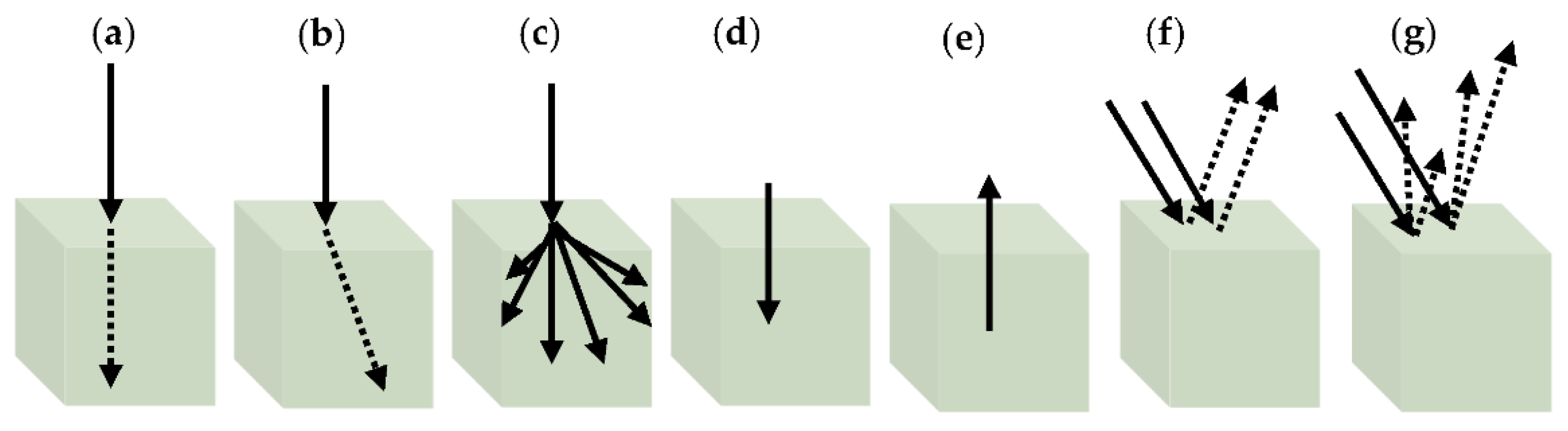
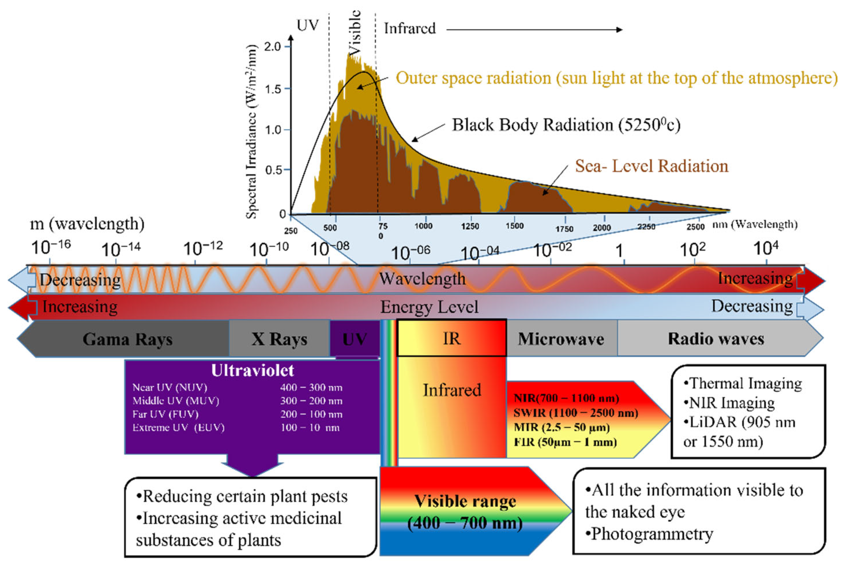
2.2. Electromagnetic Spectrum

Remote sensing technology depends on the measurement and interpretation of EMR arrays. This radiation carries specific electrical and magnetic properties. We refer to the wavelength range that corresponds to the electromagnetic radiation as the electromagnetic spectrum. We can use the manner of the interaction between the electromagnetic spectrum with any material for the qualitative and quantitative analyses of various materials. Researchers often use the electromagnetic spectrum to analyze the various chemical and physical properties of food and agriculture materials [23]. The electromagnetic spectrum ranges from shorter wavelengths (including gamma and X-rays) to longer wavelengths (including microwaves and broadcast radio waves), as detailed in

Table 1. Broad categorization of the electromagnetic spectrum.

Broad Category	Wavelength (m) (Low to High)	Frequency (Hz) (High to Low)
Gamma radiation	$<{10}^{-11}$	$>3\times {10}^{19}$
X-ray radiation	${10}^{-9}-{10}^{-11}$	$3\times {10}^{17}-3\times {10}^{19}$
Ultraviolet radiation	$4\times {10}^{-7}-{10}^{-9}$	$7.5\times {10}^{14}-3\times {10}^{17}$
Visible radiation	$7\times {10}^{-7}-4\times {10}^{-7}$	$4.3\times {10}^{14}-7.5\times {10}^{14}$
Infrared radiation	$1\times {10}^{-5}-7\times {10}^{-7}$	$3\times {10}^{12}-4.3\times {10}^{14}$
Microwave radiation	$0.01-{10}^{-5}$	$3\times {10}^9-3\times {10}^{12}$
Radio waves	$>0.01$	$<3\times {10}^9$

. The three basic factors that define the electromagnetic spectrum are the frequency (f), wavelength (λ), and photon energy (E). The frequency refers to the number of cycles per unit time, which are measured in hertz (Hz) (number of cycles per second). The wavelength refers to the distance between two successive cycles, which is measured in meters (m), and which is inversely proportional to the frequency. The following equations describe the relationships between the frequency, wavelength, and energy:

$$f=\frac{c}{\lambda },$$

(1)

$$f=\frac{E}{h} ,$$

(2)

$$E=\frac{hc}{\lambda } ,$$

(3)

where h is the Planck’s constant (6.6206957 × 10⁻³⁴), and c is the speed of light in a vacuum (299,792,458 m/s).

Depending on the type of interaction with the object (Figure 1), we can use the electromagnetic spectrum in different types of spectroscopic techniques to study material properties. The most applied interaction types for agricultural applications include reflectance, where the radiation is bounced back in either regular or irregular directions; ab-sorption, where the electromagnetic radiation is absorbed by the object (e.g., in photosynthesis); transmission, where the object allows the passage of electromagnetic radiation; emission, where the object emits the electromagnetic radiation that is the result of an energy state transition (e.g., fluorescence).

The different categories of electromagnetic spectra (Table 1) have several applications in agricultural production chains. Although we focus on field crop monitoring in this paper, we present a brief overview and summary of the general applications of electromagnetic spectra with respect to the agricultural production value chain. In this article, the value chain includes in-field operations, product processing, and consumption.

2.2.1. Gamma-Ray Imaging and Spectroscopy

Gamma rays are quanta or photons of extremely high frequency, low wavelengths, and high-energy electromagnetic radiation that are emitted from naturally occurring iso-topes. This radiation is ionizing, and it has high energy and is capable of penetration for effective irradiation. The radioactive isotopes of the elements that are capable of emitting gamma radiation are called radionuclides. Most radionuclides naturally occur, except for potassium (K) and the decay series of uranium (U) and thorium (Th), which produce gamma rays with sufficient energy and intensity that we can measure them with gamma-ray spectroscopy [24]. Researchers have found these radionuclides in soils and rocks in varying amounts. For this reason, gamma-ray spectroscopy is applied in agricultural production processes to characterize the soil properties for arable farming. Mahmood [25] adopted proximal gamma-ray spectroscopy to predict several soil properties using windowed and full-spectrum analysis methods under both managed soil conditions and a conventional field. Their methods could be used to predict the clay, pH, and total nitrogen with good precision (R² ≥ 0.56) in managed soil, whereas they could only be used to predict the total nitrogen with good accuracy in an organic field. Thus, they concluded that gamma-ray spectroscopy can be used for soil characterization for which the seedbed condition is important, although it cannot be used to determine small differences in the soil structure. Strati [24] also proved the feasibility and reliability of proximal gamma-ray spectroscopy in the modeling of the soil water content in agricultural fields, considering one case study on a tomato field. Serafini [25] describes another application of proximal gamma-ray spectroscopy in precision agriculture for the discernment of the rain water and irrigation water in soil without any supporting meteorological information.

2.2.2. X-ray Imaging

X-ray radiation, which is similar to gamma radiation, has a high frequency and energy and low wavelengths, and it is often used for irradiation and plant breeding applications, as well as for soil property characterization [23]. An example application of X-ray imaging is in the topographic study of agricultural soils using X-ray fluorescence and gamma-ray spectroscopy. De Castilhos [26] used energy-dispersive X-ray fluorescence (EDXRF) and gamma-ray spectrometry data, combined with principal component analysis (PCA), to characterize the soil chemical properties and analyze the concentration variation within the topographic sequence and depth in an agricultural field. Researchers have applied portable X-ray fluorescence imaging to the evaluation of heavy metals in agricultural soils, including the reported assessment of the heavy metals and soil organic carbon, in agricultural landfills [27]. According to their results, the method can be used to predict the soil organic carbon reasonably well (validation R² = 0.7), without the depth as an auxiliary predictor. The results of this study are similar to those of [28], except that, in the latter, the authors integrated arc emission spectroscopy, but with the same aim of carrying out a rapid risk assessment of the heavy metals in agricultural soils.

With regard to Gamma-ray and X-ray imaging, it is notable that both these remote sensing applications are limited to only a short distance between the object of interest and sensing device and for a short time. To avoid confusion with wide area remote sensing, these methods of sensing are specifically referred to as proximal remote sensing. Although these techniques are commonly adopted laboratory-based studies, some recent articles project the future potential their application in the field for monitoring heavy metals in leaves. For instance, Antenozio et al. [29] demonstrated the suitability of the micro-X-ray fluorescence (μ-XRF) technique to monitor arsenic (a metalloid that is toxic to living organisms) accumulation in plants. Moreover, the study performed a detailed analysis at different stages of the development of the plant and at different plant organs. In addition, other studies show that proximal sensing techniques are useful for monitoring macro and micronutrients [30].

2.2.3. Ultraviolet Imaging and Spectroscopy

The ultraviolet (UV) region of the electromagnetic spectrum is characterized by wavelengths that are lower than those of visible light (Table 1). Ultraviolet (UV) spectroscopy has recently found increasing applications in different fields, such as food and agriculture, forensic sciences, astronomy, and microscopy [31]. In UV imaging, the viewing of the surface topology of a material without light penetration is possible, as UV light is absorbed onto the surface of the material. One of the applications of UV light is for spectroscopic imaging, for which it is used as an excitation source for the study of a given material under controlled conditions. Zhao and Nakano [32] divide UV imaging into reflected UV imaging, which is commonly applied in astronomy and forensic science, and fluorescence UV imaging, which is commonly used in molecular biology. Although the application of UV imaging and its mass adoption in agriculture is still a prominent research issue, in several studies, researchers have demonstrated its vast potential in the areas of agriculture and food products. Petal et al. [33] demonstrated the potential of a reflected UV imaging technique for the detection of hidden defects/ruptured tissues on the surfaces of mangoes.

2.2.4. Mid-Infrared Imaging and Spectroscopy

The mid-infrared region has a unique property: it provides us with the ability to detect biochemical compounds, such as the sugars and acids in leaves, as well as in other materials, such as corn, jellies, and food supplements [34]. Furthermore, the development and advancement of Fourier-transform infrared (FTIR) technology has substantially promoted the use of the mid-infrared region in the agricultural and food industries. FTIR technology, coupled with other advanced technologies, such as Raman and NIR spectroscopy, has vast applications in quality, authenticity, and adulteration detection in the food industry [35]. Additionally, mid-infrared imaging has many agricultural applications, including in the early detection of plant water stress [36], nondestructive qualitative testing of the lambda-cyhalothrin residues on vegetables [37], and prediction of the daily methane emissions of dairy cows [38], among other applications.

2.2.5. Thermal Infrared Imaging

Thermal imaging (or infrared thermography) is based on infrared thermal energy, and it is used to carry out the noncontact detection of surface temperatures by acquiring thermal variations and converting the thermal spectral reflectance into a visible image [39]. In agriculture, thermal imaging can be used for intelligent irrigation monitoring [40], aerial monitoring and the quantification of crop abiotic stresses [41], early pest infestation detection in crop lands [42], and the aerial monitoring and estimation of the evapotranspiration in agricultural fields [43], among other applications.

2.2.6. Microwave Imaging

Similar to other electromagnetic-spectrum-based imaging systems, microwave im-aging also represents a series of noninvasive and nondestructive techniques that were de-signed to sense materials or scenes to retrieve certain physical properties and/or infer in-formation about the condition of the target under study. Researchers have proposed the adoption of electromagnetic fields at microwave frequencies for inspecting unknown tar-gets or scenes [44]. In agriculture, thermal heating based on microwaves can be effectively used to disinfect food, as well as nonfood materials and soils, and (most importantly) to kill pests and bacteria. Ghavami [45] used microwave imaging to nondestructively discriminate between seeded and seedless samples of lemons and grapefruits. Some of the most recent advancements in microwave imaging techniques in agriculture include the nondestructive inspection of large-trunked trees (e.g., palms) for disease infection [46], and nondestructive crop root phenotyping to inspect for possible infections [47]. This research field has shown great potential in the estimation of the sizes of root tuber crops, such as carrots, potatoes, and onions, among others; thus, it provides a means of facilitating root tuber yield predictions.

2.2.7. Radio Wave Imaging

Radio waves, and particularly in the range from 3 kHz to 300 GHz, are commonly used in a variety of devices, including air conditioners, computer-related peripherals (e.g., wireless routers, keyboards, mice), and so on. The design and implementation of radio-based systems for food and agriculture applications has been advancing in recent years. Researchers have developed devices that work at low frequencies (e.g., less than 200 KHz) for the inspection of food products as air-coupled ultrasonic systems [48]. They have also developed technologies that utilize high frequencies (e.g., up to 210 GHz) for the imaging/detection of the materials in food products. For example, in one case study, the authors considered the imaging of crickets buried in flour [49]. In recent years, researchers have taken radio wave imaging in agriculture in various directions, such as underground soil sensing using subsurface radio wave propagation The present-day state-of-the-art technology the IoT was made possible through the ease of the networking and communication using radio waves.

2.2.8. Color and Near-Infrared Imaging and Spectroscopy

To this point, in the various abovementioned applications, the focus has been on ap-plications that use active-sensor-based systems. However, these technologies are not frequently used due to the relatively high costs of the artificial generation of the radiation and safely concerns, and especially in outdoor applications, as they are known to have harmful effects. Nonetheless, almost all commonly used remote sensing systems in agriculture are passive in nature, as they rely on naturally occurring EMR (i.e., radiation that survives atmospheric scattering and reaches the Earth’s surface), which thus lowers the associated costs. We present the electromagnetic spectrum regions that are commonly used in agricultural remote sensing for field crop monitoring in Figure 2. These regions range from the visible to near-infrared bands (400–2500 nm wavelength range).

The information associated with each region in the electromagnetic spectrum can be helpful for a particular purpose for understanding field crops. The visible spectrum (0.4–0.7 µm) is used for vision-based sensing (i.e., measures to quantify all valuable data ob-servable by the naked eye), such as chlorophyll studies, green indices, and morphological analyses of leaves and fruits [50]. Similarly, the infrared region (0.3–100 µm) is used to extract data that are hidden from the naked eye, such as the plant water content and stress-related indices [51]. However, the infrared (IR) spectrum that is used in remote sensing comprises two subcategories, based on the radiation properties: (1) the reflected IR spectrum (0.7–3.0 µm), which is used for remote sensing purposes in a similar manner to the visible spectrum; (2) the emitted or thermal IR spectrum (3.0–100 µm), which is radiation that is emitted from the Earth’s surface in the form of heat energy.

2.3. Imaging Techniques

Spectral imaging combines the conventional imaging and spectroscopic techniques into one system to produce both spatial and spectral information of a given scene. According to Xu and Mishra [52], this simplifies the simultaneous measurement of the multiple physical (e.g., size, shape, and color) and chemical (e.g., water, fat, sugar content) characteristics of the target scene(s). Spectral information reveals the spectral signature of the analyte of interest, which can be spatially visualized in the form of distribution maps. Spectral imaging data (x,y,λ) (Figure 3), which are also referred to as hypercubes, are three-dimensional (3D) data, including two spatial dimensions (x rows and y columns) and one spectral dimension (λ wavelengths). Although the field of spectral imaging has many inconsistent terminologies, such as spectral imaging and imaging spectroscopy (or imaging spectrometry), in this article, we use all three of these terms to refer to the same concept. The two major imaging techniques are multispectral imaging (MSI) and hyperspectral imaging (HSI).

2.3.1. Multi-Spectral Imaging

Multispectral imagery is composed of a few image layers of a given scene, with each layer acquired at a particular section (also called band) of the electromagnetic spectrum [53]. The most common multispectral sensors have 3–10 spectral band measurements at each pixel of the produced image. For example, Landsat 8 Operational Land Imager (OLI) and thermal infrared sensor (TIRS) images consist of nine spectral bands, with a spatial resolution of 30 m for Bands 1–7 and 9. Sentinel, Landsat, Quickbird, and Spot are well-known satellites that use multispectral sensors to produce images that are composed of bands in the wavelength range of 443–2190 nm (that is, from the ultra-blue band (coastal and aerosol studies) to the shortwave-infrared (SWIR) band) acquired at different spatial resolutions [54].

In most of the studies in the literature, the authors demonstrate the vast range of MSI applications in field crop monitoring, including the phenotyping of crop biomasses [55,56,57], influence of the reproductive organ (RO) on the crop bidirectional reflectance distribution function (BRDF) and NDVI [58], estimation of the photosynthetic pigment [58], and assessment of the nitrogen variability [59], among other applications.

Additionally, multispectral imaging has also been widely adopted in agriculture for other applications, including seed phenotyping for the purposes of seed variety/species segregation and/or quality grading [60], soil nutrient estimations in agricultural soils [61], and the monitoring of the chlorophyll contents in crops [62]. Furthermore, the use of multispectral imaging has improved the agricultural sector and the utilization of various cutting-edge technologies, such as machine-learning and big data analyses.

Despite the many MSI applications, there are some shortcomings to MSI technology, which the authors of [63] examine. One such shortcoming is the low number of discrete spectral bands that are retrieved to aid studies that extend beyond the plant indices. Researchers have also had color restoration problems (i.e., RGB representation) when using MSI due to the overlap of the visible and near-infrared spectral bands [64], among others. However, MSI remains the most applied technique in remote sensing for field crop monitoring, compared with HSI, which is because the HSI processing techniques are still largely under development.

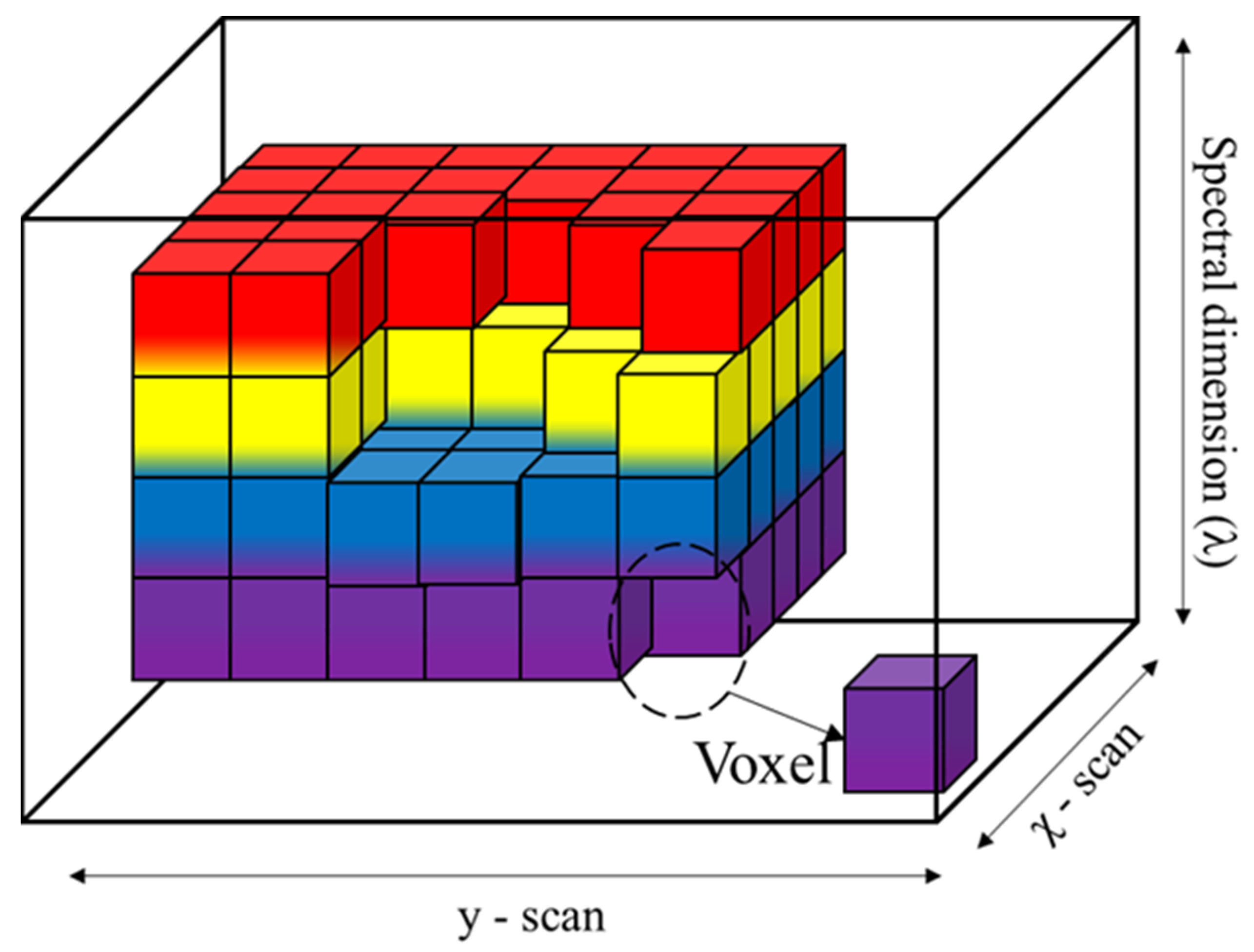
2.3.2. Hyperspectral Imaging

Unlike MSI, which collects a few image layers of the same scene, when spectral images are captured for narrow spectral bands rather than discrete bands, the system is referred to as hyperspectral imaging (HSI). These systems include sensors that collect dozens or hundreds of spectral bands with a wide range of spectral coverages [65]. Moreover, in several studies, researchers have proven that HSI technology can outperform MSI in different agricultural-based applications due to its ability to detect and discriminate between the specific features of objects with several narrow contiguous spectral channels. For example, in digital soil mapping (DSM) [66,67,68], HSI yielded more promising results due to its ability to retrieve extensive spectral signatures. Moriya et al. [69] also report a better performance for the detection of citrus gummosis with hyperspectral images than with three-band multispectral images.

Additionally, because HSI acquires an entire spectrum at each point, there is no need to have prior knowledge of the scene because all the available information in the dataset can be extracted during the postprocessing and analysis [70]. Furthermore, the latter authors point out that HIS analyses also take advantage of the structural relationships among the different spectra in a neighborhood, allowing for more elaborate spectral structural models for the more accurate analysis and classification of images.

One other problem that is associated with HSI is referred to as “smile” or “frown”. Spectral smile curves are the spectral distortion to an across-stack wavelength shift from the central wavelength owing to the change in the dispersion angle with the field position. This problem is primarily associated with push broom sensors [71], and it is visualized as a wave shape. Nevertheless, HSI has found comprehensive applications not only in remote sensing field crop monitoring and other agricultural applications, but also in other fields of research, such as medical diagnosis [72] and facial recognition [73].

2.3.3. Approaches to Spectral Imaging

Scanning Systems

Researchers use three main spectral scanning technologies to obtain spatial and spectral information: point scanning, line scanning, and band sequential scanning [74]. Spectral scanning combines the dispersive spectrometer with raster scanning. As depicted in Figure 4, point scanning captures one spectral data point at a time, while line scanning captures a slit of spatial information [75]. However, these two scanning approaches require a longer period of time to collect the data cubes [74]. Similar to the point and line scan approaches, band sequential scanning can acquire a high-resolution 2D image one wavelength at a time. While it allows for the measurement of continuous spectra, the major limitation of scanning is the high losses at the entrance slit of the spectrometer, which leads to long acquisition times.

Snapshot Systems

The snapshot approaches use a matrix of bandpass filters on the detector surface and spectral systems, which employ a tunable spectral filter in front of a monochrome imaging camera. The approaches are straightforward and can obtain both the spatial and spectral information of a scene with one exposure, which makes them superior to the former methods, as no scanning is required. However, there are three major disadvantages to snapshot technology: (1) the induced image blurring due to motion artifacts; (2) low spectral resolution; and (3) a limited number of wavelengths. For this reason, scanning devices are the most widely used instruments for collecting spectral images [76].

Fourier Transform Spectroscopy

Fourier-transform (FT) spectroscopy is an alternative approach to measuring continuous spectra. It combines a monochrome imaging sensor with an interferometer [77]. The principle behind FT spectroscopy is that light is split into two collinear delayed replicas, and a detector is used to measure their interference pattern as a function of their relative delay. The FT of the resulting interferogram produces the continuous-intensity light spectrum [78].

FT spectroscopy has many advantages over the dispersive techniques of measuring continuous spectra, which include the simultaneous measurement of all the wavelengths, and the increase in the number of photons that reach the sensor, which produces a higher signal-to-noise ratio. Another powerful advantage is the variable spectral resolution, which is adjustable, depending on the interests of the individual end user, by varying the maximum scan delay of the interferometer via software, without affecting the throughput of the device. FT spectroscopy also has a higher throughput because there are no slits, as well as a high wavelength accuracy due to the laser beam calibration of the device. Finally, it allows the user to adjust the spatial resolution independent of the spectral resolution [77]. There are many FT-based spectroscopy devices commonly in use, including the Raman spectrometer [79] and Hadamard spectrometer [80], and most of them are best suited to indoor applications (i.e., laboratory and industrial process lines) due to their designs.

Recently, there have been advancements in FT spectroscopy for outdoor applications. One of the well-known devices is the “Hera Iperspettrale” developed by NIREOS [81]. The Hera Iperspettrale utilizes a patented common-path birefringent interferometer (CPI) [82] in combination with a bidimensional CMOS sensor. The CPI is known for overcoming the limitations of the Wollaston and Savart prism-based imagers, providing negligible chromatic dispersion and the small geometrical separation between the interfering replicas, which lead to a high degree of coherence at each pixel and strong interference modulation. The data cube is measured in the time domain by step-scanning a compact ultra-stable interferometer in front of the CMOS sensor. The FT at each and every pixel of the image is then automatically computed with software, which provides the final hyperspectral data cube. The spectrum at each pixel is a continuous curve; thus, the number of bands is virtually unlimited and is not defined by the hardware but rather by the software [81]. Its capability of generating a virtually unlimited number of bands makes it superior and more powerful than most well-known hyperspectral devices, and it is thus more suitable for increasing the depth of field crop monitoring.

3. Data Processing and Analysis Techniques

In this section, our intention is to expose the reader to the vastly different processing and analysis algorithms. In this context, data processing refers to the transformation of raw datasets into valuable and usable information, whereas data analysis refers to the derivation of the intelligence from the preprocessed data itself (i.e., creating insight and new information).

3.1. Preprocessing Methods

Every raw remotely sensed data point contains a number of artifacts and errors due to the working condition of the devices, the effect of the research environment, and other factors. Correcting such anomalies and/or noises (e.g., abnormal pixels, uneven bright-ness, unwanted regions, redundant data, etc.) is called preprocessing. These noises, if un-corrected, introduce incorrect and/or unrelated signals and affect the subsequent processing. Preprocessing refers to all the actions that are taken prior to the actual data analysis process. According to Famili et al. [83], a generic way of understanding data pre-processing is as the transformation $T$of the raw data vectors $X_{ik}$ to a set of new data vectors $Y_{ij}$; (i.e., $Y_{ij}=T\left(X_{ik}\right)$). In particular, $Y_{ij}$ preserves the valuable information in $X_{ik}$, eliminates at least one of the anomalies in $X_{ik}$, and is more useful than$X_{ik}$. The valuable information comprises the components of knowledge that exist in the data, such as meaningful patterns, and the goal of the data analysis is to explore and present this information in a meaningful manner.

The preprocessing of remotely sensed images prior to image analysis is essential due to its direct and important influence on the quality of the further analysis, improving the sub-sequent data-processing efficiency. We introduce the most common preprocessing methods for solving the abnormalities associated with the spectral images in agriculture in the following subsections. We also highlight the strengths and weaknesses of each method.

3.1.1. White and Dark Calibration

White and dark calibration, which is also known as pixel-level image calibration, is performed to convert the acquired light intensity into standard reflectance/transmittance values. In laboratory setups, it is also performed to eliminate random noise signals, which are sometimes referred to as the “dark current” [84]. A standard diffuse reflectance surface with a specific reflectance and completely blocked camera lens are the most common techniques used to take white and dark reference images, respectively [85]. To convert the measured absolute reference values of each pixel to relative reference values after acquiring the white reference and dark images, we apply the following equation:

$$R=\frac{I_m-I_d}{I_w-I_d}\times R_{w },$$

(4)

where $I_m$, $I_d$, and $I_r$ are the measured raw, dark, and white reflectance values, respectively. $R$ and $R_r$ are the calibrated relative reflectance value and reflectance factor of the white panel, respectively.

3.1.2. Compression of Data Size

As a way of improving the spectral resolution and removing redundant signals, re-searchers primarily utilize data size compression (i.e., increasing or reducing the dimensionality of the data) based on some predefined conditions. Spectral imaging often results in large-data-dimensional spaces, such as hyperspectral images, with up to several hundred (or even several thousand or millions in some cases) of pixels. These massive data cubes call for computationally powerful hardware machines, such as GPU-powered computers. According to the authors of [86], leaving this large dimensionality unchecked results in a phenomenon known as the curse of dimensionality (also called the Hughes effect). As a criterion, when the number of spectral channels is greater than one-third of the difference in the sample number and classes, then overfitting issues are likely to occur [87]. As a result, spectral data size compression, and particularly spectral dimensionality reduction, is essential to reducing the overfitting risk, saving storage space, and accelerating the computation. Many methods are used to achieve the size reduction goal, including cropping out rows and columns that do not contain useful information, pixel binning, and feature selection and extraction.

Pixel Binning

Binning is the process used to combine multiple pixel charges collected by several adjacent CCD pixels in the horizontal, vertical, or both directions into a single larger charge, which is known as the binned pixel (or superpixel) [88]. For example, take n and m to be the numbers of pixels that form superpixels in the vertical and horizontal directions, respectively; the binning process returns a single binned pixel, which increases the signal-to-noise ratio (SNR) and reduces the computational load [89]. However, pixel binning causes a loss of the image resolution that is equal to the binning level; thus, there is a tradeoff between increasing the SNR and losing resolution, for which a decision must be made [90].

Feature Selection and Extraction

To remove the redundant or irrelevant information from the original data, the isolation of several representative variables or features is essential. In the case of spectral images, feature selection (FS) is the process of identifying a subset of informative wavebands in an attempt to reduce the dimensionality and improve the accuracy in the subsequent image analysis, such as classification or regression, which requires the band selection, which is a challenging task, and which requires prior knowledge of the data at hand. To avoid a subjective selection, researchers have developed several mathematically proven methods to aid in the decision making, which include forward feature selection, Fisher scores, and ranking. Ranking is the commonly applied technique in spectral FS, as it al-lows for the sorting of all the wavebands according to certain criteria and the selection of those with large weight coefficients. According to the authors of [90], the obtained weight coefficients can be treated as the loadings for the principal component analysis (PCA) regression coefficients of calibration models [91], and correlation coefficients between new variables and targets [92], among others.

In contrast to FS that is aimed at isolating only the representative variables, feature extraction (FE) methods can be used to transform the original data into a new low-dimensional coordinate system using the original features/variables. Despite the fact that FE methods require all the original data in the analysis process, unlike FS methods, they still achieve higher classification accuracy [93]. The transformation of the original data into a new feature space is performed through projections, such as orthogonal centroid algorithms (OCAs), projection pursuit (PP), PCAs, minimum noise fraction (MNF), and independent component analyses (ICAs) [94]. Among these methods, the PCA algorithm is the most common method for both FS and FE in the preprocessing of spectral images (especially HSI). In PCA, a multivariate data matrix (X) is transformed into a new coordinate system to produce new uncorrelated orthogonal variables, which are referred to as principal components (PCs) or loadings (W). The PCs are automatically arranged in a descending order of dominance based on the associated eigenvalues such that the first PC contains the greatest variance, followed by the second, third, and so on [95]. To calculate the new PC score matrix (T), we use a mathematical expression: $\mathrm{T}=\mathrm{WX}$.

Because most of the useful information is contained in the first few PCs, the removal of PCs with small variances can eliminate redundant and unnecessary information. However, useful information and noise cannot be completely separated using PCs; thus, decreasing the number of PCs can cause the loss of useful information, whereas retaining too many PCs will retain the noise as well [93]. In the 1960s, researchers proposed solutions, such as using the eigenvalues according to the Kaiser criterion [96], or the scree test [97] to determine the number of PCs to retain for further analysis. Kaiser proposed keeping the eigenvalues equal to or greater than one in order to retain as much useful information as possible, whereas Cattell proposed the scree test to identify the point at which the smooth decrease in the eigenvalues appears to the right.

Another commonly used method to minimize noise before size compression is the spectral derivative categorized under the spectrum pretreatment approaches. The most commonly applied spectral derivative method is the Savitzky–Golay (SG) derivation algorithm [98], which is a method that uses a polynomial $p\left(x\right)$ to approximate the original spectral curve while minimizing the noise:

$$p\left(x\right)={{\displaystyle \sum }}_{i=0}^d{a}_i{x}^i,$$

(5)

The method uses the concept of a rolling window; thus, the increase in the order of the polynomial must be accompanied by an appropriate increase in the window width or else the produced polynomial will simply follow the noise oscillation. One other spectral derivative algorithm in the literature that minimizes the noise in spectral data is the Norris–Williams (NW) derivation [99]. Other spectrum pretreatment methods include multiplicative scatter (MSC) and standard normal variate (SNV), which are generally categorized as scatter correction approaches [100].

In addition to the abovementioned image calibration, size compression, and spectrum pretreatment approaches, another preprocessing technique is spectral unmixing (SU). SU is the procedure by which the measured spectrum of a mixed pixel is decom-posed into a cluster of constituent spectra (or endmembers) and a set of corresponding fractions or abundances that indicate the proportion of each endmember present in the pixel [101]. Unlike the abovementioned preprocessing methods, studies in which researchers apply SU to the analysis of spectral data in agriculture are few.

One other powerful preprocessing method for field crop monitoring is tasseled cap transformation [102], which was designed to analyze and map the vegetation and urban development changes detected by various satellite sensor systems. The transformation has several advantages, including a reduction in the amount of data from several multispectral bands to three primary components: brightness, greenness, and wetness (or yellow stuff for Landsat MSS), as well as a reduction in the atmospheric influences and noise components in the imagery, which enables a more accurate analysis. A unique characteristic of PCA is that it can be used to transform the image data into a new coordinate system with a new set of orthogonal axes. The brightness axis (primary axis), which is statistically derived, is calculated as the weighted sum of the reflectance of all the spectral bands, and it accounts for most of the variability in the image. The brightness is influenced by bare or partially covered soil and other manmade and natural features. The second axis orthogonal to the first axis is the greenness axis, which is associated with green vegetation, while the third axis, wetness, is orthogonal to the first two axes and is associated with the soil moisture, water, and other moist features.

Finally, in addition to the abovementioned classical approaches, image cleaning is a conventional approach to spectral data preprocessing. Generally, measured images of all the objects within the rectangular camera’s field of view are retrieved and not just the tar-get object(s), which means that the image contains other redundant and irrelevant regions. These irrelevant regions include, among others, the background and labels. Other artifacts are induced by specular reflection and the environmental and device conditions. There-fore, dealing with these unwanted pixels and regions is essential, as they can cause incorrect or unrelated signals and consequently affect the subsequent analysis. The methods that are used to deal with these artifacts include manual selection, thresholding, image filtering, and interactive selection [103].

3.2. Analysis Methods

For decades, there have been developments and advancements in the remote collection of information on and images of the Earth’s surface and the atmosphere using aircraft and satellites. The collection of this information enables the characterization of the natural features or physical objects on the ground, the observation of surface areas and objects on a systematic basis and the monitoring of their changes over time, and the ability to integrate these data with other information as a decision-making aid. Analyses of remote sensing data can enhance our understanding of the terrestrial surface or particular areas of interest in terms of the composition, form, and function. Over the years, the need for computer-based analyses of remotely sensed image data has been increasing, along with the increasing volumes and types of digital image data that are available from various platforms and sensors. Therefore, according to Tüshaus et al. [104], the effective utilization of remote sensing image data necessitates the construction of an accurate means of extracting the information that they contain in forms that are relevant to particular applications. In this section, we survey the most common analysis methods that are relevant to field-crop-monitoring applications, which include vegetation indices and machine-learning and deep-learning approaches.

3.2.1. Vegetation Indices

The remote sensing of vegetation using passive sensors provides information on the electromagnetic wave reflectance from canopies in the form of spectral reflectance signatures [105]. These signatures carry information about the state, biogeochemical composition, and structure of a leaf area and/or canopy [106]. Consequently, we normally calculate vegetation indices (VIs) as the ratio of two wavebands to differentiate an absorbing feature from a nonadsorbing reference feature. For example, VIs may provide a measure of the canopy greenness, which is influenced by several biophysical quantities related to the chlorophyll content and leaf area of the canopy [106].

Multispectral Vegetation Indices

The first vegetation index proposed in the literature was the ratio vegetation index (RVI) [107]. Vegetation indices are based on the principle that leaves absorb relatively more red than infrared light. The major RVI application is for biomass estimations and monitoring, and usually for those with high-density coverages, as this index is sensitive to vegetation and can be easily correlated with the plant biomass. According to this study, the RVI is sensitive to the atmospheric effect when the vegetation cover is scarce (less than 50% cover), which weakens its representation of the biomass.

Later, the authors of [108] proposed the difference vegetation index (DVI) to determine the changes in the soil background. Researchers developed several vegetation indices in the 1970s for different applications, including the normalized difference vegetation index (NDVI), which is a typical parameter for analyzing ground differences and crop development processes. The NDVI quantifies the crop reflectance characteristics by measuring the difference between the near-infrared and red bands. However, factors such as the soil brightness, canopy coverage, and shadow affect the NDVI results, so sensor calibration is required [105]. The NDVI is the most common index, and we mathematically calculate it as follows:

$$NDVI=\frac{R+NIR}{R-NIR} .$$

(6)

Up to this point, vegetation indices could not account for the atmospheric effects on the output of the scene analysis. Vegetation indices in which the atmospheric effects are considered started to emerge in the early 1990s. The first vegetation index in which the atmospheric effects were considered was the atmospherically resistant vegetation index (ARVI), proposed by the authors of [109]. This index is effective at reducing the dependence of the vegetation indices on the atmospheric effects, as quoted in the study. However, with the advent of UAVs, the effect of the atmospheric influence on the vegetation indices was substantially minimized, which then led to the emergence of several modified vegetation indices [105]. Researchers widely apply vegetation indices that are based on UAV remote sensing in agriculture due to their ability to intensify the visible light and NIR spectral reflectance differences for improved crop monitoring (

Table 2. Spectral vegetation indices for field crop monitoring (three indices considered under each category and/or sub-category).

Category	Type	Vegetation Index Name	Formula	Property Measured	References
Basic vegetation index	Ratio Vegetation index	Ratio vegetation index (RVI)	$\mathrm{RVI}=\frac{NIR}{R}$	Chlorophyll content	[110]
		Green Ratio Vegetation Index (GRVI)	$\mathrm{GRVI}=\frac{NIR}{G}$	Nitrogen content	[105]
		Chlorophyll index with red edge (CIrededge)	$\mathrm{CIrededge}=\frac{NIR}{REG}+1$	Chlorophyll content & Leaf area index	[111]
	Difference vegetation index	Difference vegetation index (DVI)	$\mathrm{DVI}=\mathrm{NIR}-\mathrm{R}$	Chlorophyll content	[110]
		Green difference vegetation index (DVIGRE)	$\mathrm{DVIGRE}=\mathrm{NIR}-\mathrm{G}$	Chlorophyll content	[110]
		Red edge difference vegetation index (DVIRED)	$\mathrm{DVIGRE}=\mathrm{NIR}-\mathrm{REG}$	Chlorophyll content	[110]
Functional vegetation index	Atmospherically adjusted vegetation index	Atmospherically resistant vegetation index (ARVI)	$\mathrm{AVRI}=\frac{\mathrm{NIR}-R_{RB}}{\mathrm{NIR}+R_{RB}}$ $R_{RB}=R-\gamma \left(R-B\right)$	-	[112]
		Green Atmospherically Resistant Index (GARI)	$\mathrm{GARI}=\frac{\mathrm{NIR}-\mathrm{G}+1.75\left(\mathrm{B}-\mathrm{R}\right)}{\mathrm{NIR}+\mathrm{G}-1.75\left(\mathrm{B}-\mathrm{R}\right)}$	Chlorophyll	[112]
		Visible Atmospherically Resistant Index (VARI)	$\mathrm{VARI}=\frac{\mathrm{G}-\mathrm{R}}{\mathrm{G}+\mathrm{R}-\mathrm{B}}$	Biomass	[113]
	Soil-adjusted vegetation index	Soil-adjusted vegetation index (SAVI)	$\mathrm{SAVI}=\frac{1.5\left(\mathrm{NIR}-\mathrm{R}\right)}{\mathrm{NIR}+\mathrm{R}+0.5}$	Nitrogen	[114]
		Optimized soil-adjusted vegetation index (OSAVI)	$\mathrm{OSAVI}=\frac{1.16\left(\mathrm{NIR}-\mathrm{R}\right)}{\mathrm{NIR}+\mathrm{R}+0.16}$	Chlorophyll	[112]
		Modified Soil-Adjusted Vegetation Index (MSAVI)	$\mathrm{MSAVI}=\frac{1.5\left(\mathrm{NIR}-\mathrm{R}\right)}{\mathrm{NIR}+\mathrm{R}}+0.5$	Chlorophyll	[112]
Modified vegetation index		Normalized difference vegetation index (NDVI)	$\mathrm{NDVI} =\frac{\mathrm{NIR}-\mathrm{R}}{\mathrm{NIR}+\mathrm{R}}$	Chlorophyll content	[115]
		Modified simple ratio (MSR)	$\mathrm{MSR} =\frac{\frac{\mathrm{NIR}}{R-1}}{{\left(\frac{\mathrm{NIR}}{R+1}\right)}^{0.5}}$	Chlorophyll content	[115]
		Normalized difference red edge (NDRE)	$\mathrm{NDRE} =\frac{NIR-REG}{NIR+REG}$	Nitrogen	[116]

Note: NIR, Near-infrared; R, Red; G, Green; REG, red-edge; and B, blue are the reflectance bands with wavelengths of 800–2500 nm, 620–50 nm, 495–570 nm, 700–800 nm, and 450–495 nm, respectively.

).

Hyperspectral Vegetation Indices

The abovementioned VIs are mainly suited to MSI, which provides low-resolution spectral information for fine-scale field crop monitoring. HSI is now available and is be-coming more popular because it provides hundreds of fine contiguous spectral bands that range from visible to infrared light. The first proposed HSI-based VIs were the red-edge-position (REP) VI [117], normalized pigment chlorophyll ratio index (NPCI) [118], and modified chlorophyll absorption in reflectance index (MCARI) [119], among others. These VIs have the same working concepts as multispectral-based VIs. However, in recent years, researchers have made advancements in the newly developed hyperspectral indices that are based on spectra curve areas and transformed spectra, such as the first-derivative, reciprocal, and logarithmic transformations.

For example, in order to effectively monitor the LAI of rice, the authors of [120] conducted multiple spectral transformations and vegetation index calculations using hyperspectral data, filtered the characteristic bands associated with the LAI using different processing methods, established three different models for comparison, and came up with the optimal monitoring model. According to their results, the correlation between the canopy spectrum and LAI was substantially improved after the first-derivative transformation.

The authors of [121] estimated the chlorophyll contents of crops from hyperspectral data using a normalized area over reflectance curve (NAOC). The index is based on the calculation of the area over the reflectance curve obtained by high-spectral-resolution reflectance measurements derived from the integral of the red–near-infrared interval divided by the maximum reflectance in that spectral region. According to their results, there was a linear correlation between the NAOC and leaf chlorophyll content. The method offers a simple way of estimating the leaf chlorophyll from a remote sensing hyperspectral image in a heterogeneous scene that is characterized by different crop and soil types, without the need for additional ground measurements. Thus, a single hyperspectral image is enough to establish a map of the leaf chlorophyll. Other VIs that are suited to hyperspectral images include those found in [122,123,124,125].

3.2.2. Machine Learning

Machine learning is a subset of artificial intelligence that involves the use and/or development of algorithms and statistical models that can learn from data and improve their performance over time on a specific task without being explicitly programmed. There are several different classes of machine learning algorithms, which can be broadly categorized based on the type of learning they perform: (1) Supervised learning algorithms, (2) Unsupervised learning algorithms, (3) Semi-supervised learning algorithms, and (4) Reinforcement learning algorithms. Furthermore, within these broad categories, machine learning can be subcategorized (based on the transformation approach used) into linear and nonlinear transformation regression algorithms (see Table 3).

Linear transformation regression algorithms are a type of machine learning algorithm that models the relationship between a dependent variable (also known as the response variable) and one or more independent variables (also known as the predictor variables) using a linear function. Thus, the model assumes that the relationship between the variables is linear, which means that the change in the dependent variable is directly proportional to the change in the independent variable(s).

There are several different types of linear regression algorithms that have been developed and used in the literature, including:

• Simple linear regression: This is the most basic type of linear regression, in which there is only one independent variable. It involves finding the values of the parameters that minimize the sum of the squared residuals (the difference between the observed value and the predicted value) for all observations in the data. It is used to model the relationship between two continuous variables, such as the prediction of crop yield based on the different amounts of fertilizer application.
• Multiple linear regression: This is a more general form of linear regression that allows for multiple independent variables. It is used to model the relationship between a dependent variable and several independent variables, for instance, assessing various factors that impact crop yield, such as soil nutrient levels, temperature, and precipitation.
• Ridge regression: This is a regularized form of linear regression that introduces a penalty term for large values of the regression coefficients. It is used to prevent overfitting and improve the generalizability of the model. Ridge regression is often used in situations where there are a large number of independent variables, and the risk of overfitting is high.
• Lasso regression: This is another regularized form of linear regression that introduces a penalty term for large values of the regression coefficients. Unlike ridge regression, which penalizes all large coefficients equally, lasso regression performs “feature selection” by setting some coefficients to zero, effectively eliminating them from the model. Lasso regression is often used in situations where there are many independent variables and some of them are not important for predicting the dependent variable.

On the other hand, nonlinear transformation regression algorithms comprise a machine learning algorithm that models the relationship between the dependent and independent variables using a nonlinear function. This means that the model does not assume a linear relationship between the variables, and the change in the dependent variable may not be directly proportional to the change in the independent variable(s). Nonlinear transformation regression algorithms can be more flexible and accurate than linear transformation algorithms when the relationship between the variables is more complex.

There are also several different types of nonlinear regression algorithms that have been developed and used in the literature, including:

• Polynomial regression: This is a type of nonlinear regression in which the relationship between the dependent variable and the independent variables is modeled using a polynomial function. Examples include quadratic regression (a second-order polynomial), cubic regression (a third-order polynomial), and higher-order polynomial regression.
• Exponential regression: This is a type of nonlinear regression in which the relationship between the dependent variable and the independent variables is modeled using an exponential function. Examples include linear exponential regression, logarithmic exponential regression, and power exponential regression.
• Logistic regression: This is a type of nonlinear regression that is used for binary classification, where the dependent variable can take on only two values (e.g., 0 or 1). It is used to model the probability regarding whether a given phenomenon is true (e.g., the probability that an image pixel belongs to a certain class).
• Neural networks: These are a type of nonlinear regression algorithm that are based on the structure and function of the human brain. They consist of multiple interconnected “neurons” that can learn complex relationships between the input variables and the output variable.
• Kernel regression: This is a type of nonlinear regression that uses a kernel function to model the relationship between the dependent variable and the independent variables. It is often used in situations where the data are not linearly separable.
• Gaussian process regression: This type of nonlinear regression uses a Gaussian process to model the relationship between the dependent variable and the independent variables. It is a Bayesian approach that can be used to model complex, nonlinear relationships and make probabilistic predictions about the output variable.

There are many applications of machine learning in various agricultural disciplines. For example, in the field of crop monitoring, machine learning algorithms can be used to analyze data from remote sensing technologies, such as satellite imagery and spectral imaging, to predict and monitor various crop characteristics, including yield, quality, and pests and diseases. Machine learning algorithms can also be used to optimize irrigation and fertilization strategies, or to improve the efficiency of precision farming techniques.

Remotely sensed data processing and analysis have been greatly enhanced with the development of machine-learning (ML) approaches due to their ability to handle both linear and nonlinear problems [126]. In general, their main areas of application are classification, clustering, regression, and dimension reduction [127]. Specifically, agriculture has substantially benefited from the intrinsic capabilities of ML to enhance on-farm activities, such as field crop monitoring [128,129]. Machine learning comprises algorithms that are capable of learning from data without being explicitly programmed. In this section, we present a detailed discussion on the three broad categories of machine learning: unsupervised, supervised, and reinforcement learning.

Table 3. Most common machine learning approaches to hyperspectral image analysis for field crop monitoring.

Algorithm Name	Learning	Transformation Approach	Sample Studies	Performance	References
Support vector machine	Supervised	Nonlinear	Support Vector Machines for crop/weed identification in maize fields	93.1%	[130]
			Quantification of Nitrogen Status in Rice by Least Squares Support Vector Machines and Reflectance Spectroscopy	94.2%	[131]
			Detection of scab in wheat ears using in situ hyperspectral data and support vector machine optimized by genetic algorithm	75.0%	[132]
Decision tree	Supervised	Nonlinear	Mapping Cynodon Dactylon Infesting Cover Crops with an Automatic Decision Tree-OBIA Procedure and UAV Imagery for Precision Viticulture	89.8%	[133]
			Automation and integration of growth monitoring in plants (with disease prediction) and crop prediction	>95.0%	[134]
			Greenness identification based on HSV decision tree	−	[135]
Random forest	Supervised	Nonlinear	Predicting Biomass and Yield in a Tomato Phenotyping Experiment Using UAV Imagery and Random Forest	−	[136]
			An Automatic Random Forest-OBIA Algorithm for Early Weed Mapping between and within Crop Rows Using UAV Imagery	87.9%	[133]
			Predicting Canopy Nitrogen Content in Citrus-Trees Using Random Forest Algorithm Associated to Spectral Vegetation Indices from UAV-Imagery	R2 = 0.9	[137]
K-nearest neighbors	Supervised	Nonlinear	Estimation of nitrogen nutrition index in rice from UAV RGB images coupled with machine learning algorithms	R2 > 0.5	[138]
			Performance Analysis of k-Nearest Neighbor Method for the Weed Detection	>93.0%	[139]
			Early Weed Detection Using Image Processing and Machine Learning Techniques in an Australian Chili Farm	63.0%	[140]
Naïve Bayes	Supervised	Linear	AI Crop Predictor and Weed Detector Using Wireless Technologies: A Smart Application for Farmers	89.3%	[141]
			Identification of Soybean Foliar Diseases Using Unmanned Aerial Vehicle Images	95.0%	[142]
			Naïve Bayes Classification of High-Resolution Aerial Imagery	94.0%	[143]
Logistic regression	Supervised	Nonlinear	Biomass Estimation Using 3D Data from Unmanned Aerial Vehicle Imagery in a Tropical Woodland	R2 = 0.65	[144]
			The Predictive Power of Regression Models to Determine Grass Weed Infestations in Cereals Based on Drone Imagery—Statistical and Practical Aspects	83.0%	[145]
			Automation solutions for the evaluation of plant health in corn fields	79.2%	[146]
Linear discriminant analysis	Supervised	Linear	Weed detection with Unmanned Aerial Vehicles in agricultural systems	87.0%	[147]
			Using continuous wavelet analysis for monitoring wheat yellow rust in different infestation stages based on unmanned aerial vehicle hyperspectral images	−	[148]
K-means clustering	Unsupervised	Linear	Rice yield estimation based on k-means clustering with graph-cut segmentation using low-altitude UAV images	67.0%	[149]
			Wheat ear counting using k-means clustering segmentation and convolutional neural network	>98.0%	[150]
			Detection of tomatoes using spectral-spatial methods in remotely sensed RGB images captured by UAV	88.2%	[151]
Principal component analysis	Unsupervised	Linear	Use of principal components of UAV-acquired narrow-band multispectral imagery to map the diverse low stature vegetation fraction of absorbed photosynthetically active radiation (fAPAR)	77.0%	[152]
			The Extraction of Wheat Lodging Area in UAV’s Image Used Spectral and Texture Features	87.0%	[153]
			Monitoring Agronomic Parameters of Winter Wheat Crops with Low-Cost UAV Imagery	0.7 < R2 < 0.97	[154]
Independent component analysis	Unsupervised	Linear	Field heterogeneity detection based on the modified Fast ICA RGB-image processing	78.0–89.0%	[155]
Gaussian Process Regression	Supervised	Nonlinear	Biomass estimation in batch biotechnological processes by Bayesian Gaussian process regression	−	[156]
			Spectral band selection for vegetation properties retrieval using Gaussian processes regression	79.0–95.0	[157]

Table 3. Most common machine learning approaches to hyperspectral image analysis for field crop monitoring.

Algorithm Name	Learning	Transformation Approach	Sample Studies	Performance	References
Support vector machine	Supervised	Nonlinear	Support Vector Machines for crop/weed identification in maize fields	93.1%	[130]
			Quantification of Nitrogen Status in Rice by Least Squares Support Vector Machines and Reflectance Spectroscopy	94.2%	[131]
			Detection of scab in wheat ears using in situ hyperspectral data and support vector machine optimized by genetic algorithm	75.0%	[132]
Decision tree	Supervised	Nonlinear	Mapping Cynodon Dactylon Infesting Cover Crops with an Automatic Decision Tree-OBIA Procedure and UAV Imagery for Precision Viticulture	89.8%	[133]
			Automation and integration of growth monitoring in plants (with disease prediction) and crop prediction	>95.0%	[134]
			Greenness identification based on HSV decision tree	−	[135]
Random forest	Supervised	Nonlinear	Predicting Biomass and Yield in a Tomato Phenotyping Experiment Using UAV Imagery and Random Forest	−	[136]
			An Automatic Random Forest-OBIA Algorithm for Early Weed Mapping between and within Crop Rows Using UAV Imagery	87.9%	[133]
			Predicting Canopy Nitrogen Content in Citrus-Trees Using Random Forest Algorithm Associated to Spectral Vegetation Indices from UAV-Imagery	R2 = 0.9	[137]
K-nearest neighbors	Supervised	Nonlinear	Estimation of nitrogen nutrition index in rice from UAV RGB images coupled with machine learning algorithms	R2 > 0.5	[138]
			Performance Analysis of k-Nearest Neighbor Method for the Weed Detection	>93.0%	[139]
			Early Weed Detection Using Image Processing and Machine Learning Techniques in an Australian Chili Farm	63.0%	[140]
Naïve Bayes	Supervised	Linear	AI Crop Predictor and Weed Detector Using Wireless Technologies: A Smart Application for Farmers	89.3%	[141]
			Identification of Soybean Foliar Diseases Using Unmanned Aerial Vehicle Images	95.0%	[142]
			Naïve Bayes Classification of High-Resolution Aerial Imagery	94.0%	[143]
Logistic regression	Supervised	Nonlinear	Biomass Estimation Using 3D Data from Unmanned Aerial Vehicle Imagery in a Tropical Woodland	R2 = 0.65	[144]
			The Predictive Power of Regression Models to Determine Grass Weed Infestations in Cereals Based on Drone Imagery—Statistical and Practical Aspects	83.0%	[145]
			Automation solutions for the evaluation of plant health in corn fields	79.2%	[146]
Linear discriminant analysis	Supervised	Linear	Weed detection with Unmanned Aerial Vehicles in agricultural systems	87.0%	[147]
			Using continuous wavelet analysis for monitoring wheat yellow rust in different infestation stages based on unmanned aerial vehicle hyperspectral images	−	[148]
K-means clustering	Unsupervised	Linear	Rice yield estimation based on k-means clustering with graph-cut segmentation using low-altitude UAV images	67.0%	[149]
			Wheat ear counting using k-means clustering segmentation and convolutional neural network	>98.0%	[150]
			Detection of tomatoes using spectral-spatial methods in remotely sensed RGB images captured by UAV	88.2%	[151]
Principal component analysis	Unsupervised	Linear	Use of principal components of UAV-acquired narrow-band multispectral imagery to map the diverse low stature vegetation fraction of absorbed photosynthetically active radiation (fAPAR)	77.0%	[152]
			The Extraction of Wheat Lodging Area in UAV’s Image Used Spectral and Texture Features	87.0%	[153]
			Monitoring Agronomic Parameters of Winter Wheat Crops with Low-Cost UAV Imagery	0.7 < R2 < 0.97	[154]
Independent component analysis	Unsupervised	Linear	Field heterogeneity detection based on the modified Fast ICA RGB-image processing	78.0–89.0%	[155]
Gaussian Process Regression	Supervised	Nonlinear	Biomass estimation in batch biotechnological processes by Bayesian Gaussian process regression	−	[156]
			Spectral band selection for vegetation properties retrieval using Gaussian processes regression	79.0–95.0	[157]

Supervised Machine Learning

Supervised machine learning involves training a model using labeled data, which then helps in the classification and/or prediction of future data. According to the authors of [158], the labeled data guide the machine to search for a specific pattern in the data; thus, supervised learning implies the use of a sample set in which the output is known. Classification and regression are the major subdomains of supervised learning. The tools that are commonly applied to achieve the tasks in this subdomain include support vector machines, decision trees, random forests, logistic regression, naïve Bayes, linear discriminant analyses, and artificial neural networks.

Support Vector Machine

The support vector machine is one of the most common tools in machine learning. SVMs can be used to ascertain the optimal hyperplanes that separate the points of one class from those of others due to their ability to select the planes that pass through the largest possible gaps between the points of distinct classes. The classification of the new points is then performed depending on which side of the plane they reside on. This capability of creating optimal hyperplanes also has the advantage of reducing generalization errors, and thus the chance of overfitting. However, in most studies, researchers have demonstrated that support vector machines are effective for high-dimensional spaces that require learning from several features, and the authors of [159] also found that SVMs perform equally well on relatively small datasets with few data points. Furthermore, they require less memory storage, as only a subset of points is required to represent the boundary surface. However, it should be noted that SVMs require intensive computation during the model training, and they do not return the confidence level of a prediction, which we can calculate using k-fold cross-validation [160].

In recent years, studies on field crop monitoring using support vector machines have yielded promising results, indicating their potential to improve agricultural productivity. Among these studies, the authors of [161] focused on developing a systematic model based on SVM for the monitoring of sugarcane crops. The model considers the temperature, humidity, and moisture as the monitoring parameters responsible for the healthy growth of crops, and it can also be used to detect any trace of disease infection (if any) through the aerial images acquired at regular intervals. A validation accuracy of 96% was achieved; thus, this method is reliable for the monitoring of growing crops. In another study on field crop monitoring based on SVM, the authors intended to automate the detection of crop leaf diseases from remotely sensed images [162]. The constructed algorithm achieved a good validation accuracy (87.6%), outperforming the other tested auxiliary models. Other relevant recent studies include autumn crop yield prediction using SVM [163], the detection of scab in wheat ears using HSI and SVM [132], and the identification of irrigated crop types using datasets derived from the Sentinel-2 satellite [164], among others.

Decision Trees

Decision trees are methods used for data discrimination, and they have tree-like structures with internal nodes that represent the test feature targets, of which each branch represents the result of a test, and each leaf node represents the class label. Therefore, a decision tree comprises three types of nodes: root nodes, internal nodes, and leaf nodes, and it follows a classification rule that represents the pathway from root to leaf. The decision taken at each node is based on Boolean tests. The authors of [158] describe it as a greedy algorithm, as it has a top-down iterative divide-and-rule structure. Initially, the root nodes take the entire training dataset, which is iteratively split, depending on the selected features. This process is repeated at each node, at which the test features are split based on certain decision tree functions, such as entropy and the Gini index. Entropy provides the amount of disorder in each set, and it returns zero if all the points in the target classes are the same, whereas the Gini index measures the criteria required to reduce the probability of misclassification. The algorithm result can be enhanced through a technique known as ensemble learning. Researchers widely use decision trees, as they do not require the creation of auxiliary dummy variables. However, according to the authors of [165], one major issue with decision trees is the large growth of the trees, which results in one observation per leaf. Researchers have used different spectral preprocessing techniques that employ decision tree algorithms, such as Savitzky–Golay derivatives [98], multiplicative signal correction (MSC) [166], and normalization [167], to improve the spectral features.

In the field of agricultural crop monitoring, researchers have employed decision trees in different studies, including one in which the authors focused on the greenness identification from images captured over field crops for growth monitoring [135]. A recent application of the decision tree algorithm in crop monitoring was the development of a monitoring system for the grain loss of paddy rice by the authors of [168]. Their system performed well, with an average test accuracy of 99.3% at a moisture content of 30% and a grain:impurity ratio of 1:2.5. However, as the moisture content and grain:impurity ratio increased, the accuracy of the system decreased, which implies that the optimal conditions need to be ascertained for the best possible results.

Random Forest

A random forest is a modified form of the decision tree algorithm in which a decision tree is created with a subset of training samples that are selected on a random basis with replacements. Similarly, a random number of features is also taken from each set of features. Random forests follow this process of decision tree construction many times, which results in a set of classifiers. As with decision trees, each grown tree in the random forest algorithm predicts its target class at the time of the prediction for every instance. Therefore, the class that is the most predicted by the trees becomes the suggested class of the final classifier. However, the choice of the number of parameters requires more attention. Che [169] argued that, generally, the higher the number of trees, the better the performance of the obtained classifier; however, this comes with a high computational cost. The performances of random forests are more prone to overfitting because they involve the multiple averaging of the decision trees [170]. Randal and Olson [171] suggested that a reduction in the size of the bootstrap sample, which may also increase the randomness of the algorithm, reduces the overfitting effect; however, they also mentioned that reducing the size of the bootstraps somewhat affects the overall performance of the classifier. In this regard, in most practical applications, the bootstrap size is equal to the size of the initial training set to provide a fair tradeoff between the variance and bias [133].

Researchers have employed random forests for HSI analysis in several ways, including in the detection of plant diseases, fungal infection, and bruises in fruits and vegetables, the classification of different agricultural products, and quality analyses of processed fish products [172]. In a recent study in which the authors deployed the random forest algorithm for field crop monitoring, they focused on predicting the biomasses and yields of individual tomato plants from UAV imagery [136], as the biomass and yield are fundamental variables for assessing the production and performance of agricultural crops and/or systems [136].

k-Nearest Neighbors

k-nearest neighbors (k-NN) is a machine-learning algorithm in which the classification of new cases is based on the classification of their nearest neighbors. For example, the authors of [173] state that “If it walks like a duck, quacks like a duck, and looks like a duck, then it’s probably a duck”, which means that the classification of a given pixel is based on how similar it is to its neighboring pixels. The principle that underlies k-NN classification is the k-NN rule: a test data point is assigned to the class that is most repeatedly represented among the k-nearest training data points. For cases in which two or more such classes exist, then the test data point is assigned to the class with the minimum average distance to it. The most common distance calculated in k-NN is the Euclidian distance (Frobenius); however, we can also use other distance metrics to calculate the distance points, such as the Manhattan distance (city block) and P-norm distance (Minkowsky) [174]. According to the latter study, it is important to ascertain the optimal k value to find a good balance between under- and overfitting. A small k value will render the model prone to noisy points, and if the k value is too large, then the neighborhood may encompass points from other classes. Nevertheless, the main advantages of k-NN are that the cost of the learning process is low, with no required optimization, and it is easy to program with high accuracy.

The simplicity, ease of programming, and high accuracy recorded in the literature regarding the k-NN method have greatly encouraged its adoption in different spectral analyses for field crop monitoring, such as crop canopy classification, crop disease monitoring, and crop nutrient content analyses [139]. Additionally, the k-NN method is a fast and reliable way of finding the best wavelet disintegration layer and for the effective wavelength selection of HSI data via the fusion of the wavelet basis functions and k-nearest neighbors.

Naïve Bayes

The naïve Bayes (NB) model is a probabilistic model that assumes conditional independence (i.e., Bayes’ theorem) among the predictor variables to describe the outcome probabilities of related events. At first, for each data point associated with a class, we calculate a posterior probability with the aid of the prior class probabilities and class conditional probabilities of the variables once we know the class level. We follow this by the assignment of the observation to the class with the highest posterior probability [175]. The main weakness of this algorithm is its assumption of conditional independence, which means that it is unable to learn the interactions between two predictor variables/features [158].

There have been successful applications of the NB model in HSI field crop monitoring, including in crop prediction [176] and remote sensing imagery classification [177], among others. Although in most of these studies, the authors achieved high classification accuracies (over 85%) with naïve Bayes, the authors of [158] argue that the reported classification accuracy of the NB classifier has also been lower than 75%, which indicates a weak classification model.

Logistic Regression

Researchers commonly use logistic regression (LR) to evaluate the relationship be-tween independent variables (features) and a dependent variable (label, to be predicted) by calculating the probabilities using the logistic function [178]. LR belongs to a class of discriminative models classified as supervised machine learning. Researchers primarily use it for land-cover classification in remote sensing, and particularly for pixel-wise classification; however, it also serves as a building component for more complex algorithms that use ensemble and deep learning [179]. The working principle of LR is that it models the probability distribution of a given class as the logistic function of the weighted sum of the input features. In other words, researchers employ LR for the binary classification of materials, as it returns discrete binary outcomes between 0 and 1. Logistic regression is widely used due to its accurate performance, simplicity, and ease of interpretation. However, the main disadvantage of logistic regression is that it cannot be used to model nonlinear problems for which the data are not linearly separable, and it is also prone to overfitting [145].

Linear Discriminant Analysis

Linear discriminant analysis (LDA) involves ascertaining the projection hyperplane that minimizes the interclass variance and maximizes the distance between the projected means of the classes. LDA is based on the principle of defining a lower-dimensional feature subspace in which the data point separability is optimized [180]. One advantage of using linear discriminant analysis is that a generalized eigenvalue system can be solved to obtain a solution to a given problem, which allows for the fast and massive processing of data samples. Researchers commonly use LDA in feature extraction, as it improves the computational efficiency and minimizes the level of overfitting that arises from the Hughes phenomenon in nonregularized models [181]. Although researchers commonly use LDA for binary class problems, they have also proposed its use for multiclass generalization [180].

Due to its robustness, LDA is widely used in field crop monitoring based on hyper-spectral data [180,182,183,184]. In a recent study, Alajas et al. [185] used a hybrid LDA and decision tree approach to extract useful features for the classification of healthy and diseased grape leaves and to predict the percentage of the damaged area, for which they achieved a high accuracy (over 97%).

Partial Least-Squares Discriminant Analysis

Partial least squares discriminant analysis (PLS-DA) is one of the most common incorporated supervised ML methods in the present day chemometric analysis and software packages. Barker et al. [186] describe the well-established theoretical background of PLS-DA, which is derived from the two concepts of partial least squares (PLS) and LDA. Researchers developed the PLS algorithm to linearize models with nonlinear parameters used for overdetermined regression problems [187]. The algorithm was initially implemented through the nonlinear iterative partial least squares (NIPALS) algorithm [188]. However, currently, advancements in classical multivariate statistical theories have enabled the implementation of PLS in solving well-posed eigenstructure problems that clearly exhibit the PLS strike relationships between the variance summary and score correlation. Combining the advantages of PLS and LDA (i.e., the maximization of the intergroup variability relative to the measure of the shared intragroup variability), PLS-DA is one of the most powerful tools in chemometrics.

In the field of agricultural remote sensing, Stellacci et al. [189] compared the PLS-DA model performance in the selection of the optimal hyperspectral bands to discriminate the nitrogen status in durum wheat with other statistical methods. They performed the quantification of the leaf-nitrogen concentrations on samples collected at the same locations and on the same dates, and they used them as the response variables in regressive methods. The authors demonstrated that PLS-DA is best suited for response variables. They also applied PLS-DA to map the damage from rice diseases. According to their results, the PLS-DA could classify the rice diseases at the subfield scale, with an overall accuracy of 75.62%. The authors also report that the approach was later successfully applied during a typical ecoepidemic outbreak of rice dwarf, rice blast, and glume blight in China. Other applications of PLS-DA in crop monitoring are the monitoring and characterization of crops and plants [190], the qualitative and quantitative diagnoses of the nitrogen nutrition of tea plants under field conditions [191], pest and disease detection in horticulture crops by a field robot [192], and commercial tree species discrimination from airborne hyperspectral imagery [193] among other applications.

Gaussian Process Regression (GPR)

Gaussian processes (GPs) are a type of probabilistic model that can be used for both regression and classification tasks in machine learning. They are based on the idea of using a Gaussian distribution to represent the joint distribution of the function and its inputs. GPR have a number of attractive properties, including the ability to handle input uncertainty and the ability to provide uncertainty estimates for predictions.

One of the key advantages of GPR is that they can be used to make predictions even when there is limited or noisy data available. This is because GPR takes into account the correlations between the input variables and the output variable, rather than just relying on the mean of the output variable [194]. This allows GPR to make more informed predictions, even when there is a small amount of data available, whereas the main challenges with using GPR is that they can be computationally intensive, especially when working with large datasets. However, there are a number of techniques that can be used to reduce the computational complexity of GPR, such as using approximations [194,195] or restricting the model to a subset of the data [196].

The authors of [197] discuss the various advances in the field of GPR that have been made in recent years, including new algorithms that take into account the characteristics of the signal and noise in the data, as well as techniques that use automatic relevance kernels to extract knowledge and rank features automatically.

For purposes of field crop monitoring, GPR has been applied to field crop spectral analysis in many ways; for instance, GPR was applied in the retrieval of chlorophyl content from hyperspectral reflectance data collected using an airborne system [198] and wheat leaf rust disease detection [199]. Several research surveys confirm that GPR outperforms most machine learning algorithms [199,200].

Ridge Regression

Ridge regression is one of the methods for estimating the parameters of a linear regression model, commonly used to deal with collinearity, a problem that often occurs in multiple linear regression. Ridge regression is similar to least squares regression, but it adds a penalty term to the cost function that helps to reduce the magnitude of the model coefficients. This helps to prevent overfitting and improve the generalization of the model to new data.

The key advantage of ridge regression is that it can be used to perform feature selection, since the penalty term encourages the model to give smaller coefficients to less important variables. This can be useful in situations where there are a large number of predictor variables, as it can help to reduce the complexity of the model and improve its interpretability. One of its main drawbacks is that it can be sensitive to the scale of the predictor variables, which can make it difficult to compare the importance of different variables. Additionally, ridge regression may not perform well when there are a large number of irrelevant predictor variables, as the penalty term may not be sufficient to reduce the impact of these variables on the model. At the same time, better versions of ridge regression continue to be developed within the machine learning community. For instance, the authors of [201] refined the ridge regression method by proposing new ridge parameters to improve the model performance.

In the field of crop monitoring, ridge regression has been applied in various studies including some recent studies, such as the study authored by Ahmed et al. [202], to estimate wheat yield by integrating the kernel ridge regression (KRR) method coupled with complete ensemble empirical mode decomposition with adaptive noise (CEEMDAN) and the grey wolf optimization (GWO), and that of Ji et al. [120], to quantitatively monitor leaf area index (LAI) in rice based on hyperspectral feature bands and ridge regression algorithm. Also with an airborne multispectral scanner, the authors of [203] applied Ridge Regression method to estimate the leaf chlorophyll concentration using high-resolution (2 cm) images for crop health monitoring.

Lasso Regression

Least absolute shrinkage and selection operator (LASSO) is one other type of linear regression that is used to perform variable selection (a process of selecting the most important predictor variables to include in the model). It does this by adding a penalty term to the cost function that constrains the model to give smaller coefficients to less important variables. Unlike ridge regression, which penalizes all large coefficients equally, LASSO regression performs “feature selection” by setting some coefficients to zero, effectively eliminating them from the model. The penalty term is typically a function of the L1 norm, which is the sum of the absolute values of the model coefficients [204]. The main aim of LASSO regression is to find the model coefficients that minimize the sum of the squared errors between the predicted values and the observed values, subject to the constraint that the sum of the absolute values of the coefficients is less than a certain threshold. This constraint helps to reduce the complexity of the model and improve its interpretability, particularly when there are a large number of predictor variables.

Several studies relating to field crop monitoring have investigated the applicability of LASSO in this field. For example, the authors of [205] applied LASSO regression to model crop yield prediction, and also Haumont et al. [206] adopted LASSO regression to model Leek dry-biomass and nitrogen uptake across multiple sites and growing seasons based on multispectral UAV imagery.

There are some limitations to lasso regression as well. Similar to ridge regression, LASSO regression can also be sensitive to the scale of the predictor variables [204]. Furthermore, the authors of [205] highlighted that LASSO regression may also not be effective if there are a lot of predictor variables that are not relevant to the model, as the penalty term may not be strong enough to minimize the influence of these variables on the model.

Unsupervised Machine Learning

Unsupervised machine learning encompasses all the ML techniques that do not re-quire the user to supervise the model but allow the model to work by itself to discover the patterns and information in a given dataset. Therefore, researchers primarily use them to deal with unlabeled data. Unsupervised learning models enable the performance of more complex processing tasks compared with supervised learning [207]; however, they can be more unpredictable than supervised ML methods [208]. In this section, we discuss the three most common unsupervised learning algorithms for agricultural purposes.

k-Means Clustering

k-means clustering is a partitioning-based technique for grouping based on the iterative rearrangement of the data points between clusters. Its principle of operation is that it divides the dataset variables into nonoverlapping clusters or groups based on the uncovered features to produce clusters of variables with a high level of intracluster similarity and a low level of intercluster similarity [209]. The algorithm begins by randomly selecting any centroids (i.e., average locations or arithmetic means of all the points), denoted by the symbol k. The nearest points to each centroid point are assigned to that specific cluster. This is followed by re-calculation of the new centroid by averaging the position coordinates of all the points present in that cluster. The process is iterated until convergence of the clusters occurs [210].

Its ease of implementation, efficiency of computation, and low memory requirements have made k-means clustering one of the most widely applied unsupervised machine-learning methods in the exploratory data analyses and data mining in any field of research, including hyperspectral image analyses. Additionally, k-means clustering has also been adopted as an initial step for more computationally demanding algorithms, such as Gaussian mixtures, providing an approximate separation of the data as a starting point, and minimizing the noise that is present in the dataset [209]. Some recent applications of k-means clustering in field crop monitoring include the detection and classification of the pests in crops based on proximal images. In particular, Faithpraise et al. [211] used k-means clustering for the classification of 10 pest species from images captured in the field. Wang et al. [212] applied k-means clustering to segment pests (white flies) from crop leaves as a prerequisite step for intelligent pest diagnosis. Concerning the latter study, the authors specifically applied k-means clustering to the classification of each pixel after the preliminary step of image gridding, and they used the RGB color space to preselect the potential cluster centers. Researchers have also used k-means clustering to enhance the results produced by deep-learning models [213].

Principal Component Analysis

Principle component analysis is a dimensionality reduction algorithm through which multidimensional data are reduced to a lower-dimensional space while retaining most of the useful information. The method inputs a set of possibly correlated variables to create a new set of linearly uncorrelated variables. The 1st, 2nd, …, nth coordinates of the projected data represent the highest variance, followed by the second-highest variance, and so on. Every newly retrieved coordinate is termed a principal component (PC). Of the total number of PCs obtained (which is equal to the number of original dimensions in the data), those with higher variances are chosen [214].

The key advantages of PCA are its low sensitivity to noise, low computational capacity and memory requirement, and increased efficiency, as the process takes place in a smaller dimension. However, in earlier studies, researchers found that its major disadvantage is that it makes it difficult to accurately evaluate the covariance matrix [215]. According to the latter study, Li et al. [216] reported this disadvantage in a study in which even the simplest invariance could not be captured by the PCA unless availed with such information. Nonetheless, PCAs have been widely used for field crop monitoring, both in earlier and recent years. Villez et al. [217] assessed the application of unfold PCA for online plant stress monitoring and sensor failure detection in two truss tomato plants and young apple plants grown in a greenhouse. Among the recent studies, Skotadis et al. [218] used PCA to analyze the unique response patterns generated after the exposure of the sensing array to two gas analytes to automate the real-time detection of pesticides within the scope of smart farming. Additionally, Danner et al. [219] also applied PCA to reduce the amount of input data from >200 bands to 15 components.

Independent Component Analysis

Independent component analysis (ICA) is a probability-based method that is also categorized under the dimensionality reduction machine-learning algorithms. Its main goal is to retrieve the essential maximally independent and non-Gaussian component signals from the observed mixed data signals [220]. In other words, according to Pati et al. [221], ICA is an extended PCA designed to optimize the non-Gaussian nature (or minimize the Gaussian nature) of the dataset(s). While PCA is based on the principle of the optimization of the covariance matrix of the second-order statistical data, ICA is based on the optimization of higher-order statistics, such as kurtosis; thus, it yields independent components (unlike PCA, which yields uncorrelated components). However, according to Saha [221], there are only a limited number of studies in which the researchers have applied ICA in spectral data exploration and analysis. However, from a general perspective, we can use ICA transformation to transform hyperspectral data into independent components to better complete the detection and separation of the hidden noise in the image and perform dimensionality reduction, noise minimization, anomaly detection, classification and spectral endmember extraction, and data fusion [222]. In the latter study, the authors compared the performances of different feature transforms, including the PCA, minimum noise fraction (MNF), and ICA transform, and according to their results, PCA outperformed ICA and MNF.

Reinforcement Machine Learning

Reinforcement learning is among the three elementary machine-learning categories, together with supervised and unsupervised learning. It imitates how humans and animals learn without a mentor, and it is concerned with how the software agents in a given environment are rewarded when they complete an assigned task by themselves [223]. According to Monakhova [220], reinforcement-learning tasks are commonly modeled as Markov decision processes (MDPs), which involve a 5-tuple (S,A,P,R,Ɣ), where S represents a finite set of states, A represents a finite action set, P represents the transition probability, R represents the re-ward immediately provided, and Ɣ represents the discount factor. Due to its robustness, reinforcement learning has the potential to transform the essence of automation in agriculture, as it can be used to teach robots to modify their behaviors according to the relationship between them and the surrounding environment [224]. Zhang [225] conducted a case study of such an application on fully automating the UAV aerial scouting of whole crop fields based on reinforcement learning and convolutional neural networks (CNNs) to enhance precision agriculture. The researchers designed a fully autonomous aerial surveying approach that preserves the battery life by sampling field sections to sense and predict the crop health of the whole field. When compared with the conventional nonautomated UAS scouting approach, their autonomous scouting approach sampled 40% of the field and predicted the crop health with 89.8% accuracy, substantially reducing the labor costs and increasing the agricultural profits. Other applications of reinforcement learning in the literature include autonomous greenhouse control for crop growth monitoring [225], among others.

3.2.3. Deep Learning

Deep learning is an extended (“deeper”) form of the machine-learning algorithm that researchers use to explicitly extract features from raw data for classification, clustering, regression, and detection. While there are several deep-learning networks in use, the most commonly applied network for image analysis is the convolutional neural network (CNN) [226]. Typically, the structure of a deep-learning algorithm for image analysis consists of three basic layers: convolutional layers, pooling layers, and fully connected layers. The convolutional layers are made up of kernels (filters) that are responsible for the extraction of distinct features, such as edges, from the input image. The pooling layer reduces the spatial size of the input image data and thereby reduces the computational requirements in the subsequent processes. The most common technique employed in the pooling process is max-pooling [227]. Finally, in the fully connected layer, all the nodes in the first layer of the network system are interconnected with all the nodes in the second layer. Depending on the employed network architecture (e.g., unsupervised pretrained network, CNN, recurrent neural net-work, or recursive neural network), other layers, such as gates, memory cells, activation functions, encoding/decoding schemes, and so on, can be appended to the three basic layers detailed above [228].

The use of deep-learning algorithms has substantially benefited hyperspectral imaging (

Table 4. Deep learning approaches for hyperspectral image analysis in field crop monitoring.

Category	Network Architecture	Backbone	Performance	References
Pixel-based	SegNet	VGG-16	89.8%	[229]
	FCN	AlexNet	86.7%	[231]
	DeepLabv3+	ResNet-18	97.0%	[229]
	LeNet	LeNet	92.2%	[232]
	Mask R-CNN		91.8%	[233]
	FDN-92			[234]
Object-based	Faster R-CNN	Inception-v2, VGG, ZF, ResNet-50	87.2%	[235,236]
	RetinaNet	ResNet	93.0%	[237,238]
	YOLOv3	DarkNet-53	94.0%	[237,236]
	YOLOv2	DarkNet-19	96.6%	[236,239]
	SSD	VGG-16	83.2%	[239]

). Some of the major applications in hyperspectral crop growth monitoring include the assessment of the crop water stress, crop canopy classification, crop pest detection, and the detection of disease symptoms in leaves. Deep-learning models may be either pixel-based (usually for clustering purposes) or object-based (usually for object detection (e.g., pest detection)). In terms of the pixel-based models, Der Yang [229] employed UAV images with the aid of deep-learning image processing to estimate the rice lodging over a large area of paddies. They established an image semantic segmentation model that uses two neural network architectures—FCN-AlexNet and SegNet—due to their good performances in the interpretation of objects of various sizes and their computation efficiencies. For the identification of the rice lodging from the images, they achieved F1 scores of 0.80 for the FCN-AlexNet and 0.79 for the SegNet. Similarly, researchers have applied object-based deep-learning models in field crop monitoring. In a case study, Wang [230] developed a custom triple-branch HSI–LiDAR convolutional-neural-network backbone to simultaneously extract the spatial, spectral, and elevation features of land-cover objects, including those on agricultural lands. They particularly used the single-shot-detector (SSD) architecture based on the VGG-16 backbone, and they attained a performance accu-racy of 83.2%.

3.3. Data Fusion

Remote sensing primarily provides data in four dimensions: the spatial (2D), spectral (1D), temporal (1D), and radiometric (referring to numerical precision) dimensions [240]. Recent advancements in sensors have made it possible to retrieve a wide variety of information from different materials within a given area of interest. This information ranges from spectral information obtained from passive sensors (i.e., MSI and HSI data) to height and shape information obtained from LiDAR sensors, as well as to texture, amplitude, and phase information via a synthetic aperture radar (SAR). The availability of these different forms of data from different sensors requires the integration of the diverse information that they contain to enhance the scene classification and object detection capabilities. However, according to the authors of [241], we require more efforts to automate the interpretation of remote sensing data, and especially considering the recent attempts in remote sensing data fusion.

Nonetheless, all these datasets provide different representations of the same physical scene. To handle these different representations, data fusion offers potential solutions and has been widely explored over the last decade, as researchers have attempted to determine the best possible combination of these remotely sensed datasets. Generally, all tasks that require any kind of parameter estimation derived from multisource data can benefit from the use of data fusion methods [242]. For instance, researchers commonly apply the spectral information from HSI to discriminate various materials based on their reflectance values in agricultural monitoring [243]. Likewise, we can use LiDAR image point clouds (e.g., sorghum plant phenotyping (Figure 5)) to analyze the depth, height, and volumetric information, which is useful for distinguishing objects within the same scene or different parts of the same object. Furthermore, LiDAR systems have been adopted even in marking agricultural land boundaries for the purpose of control in the system of direct payments for agriculture (Integrated Administration Control System—IACS) [244]. Therefore, the integration of all these multisource information into a single analysis pipeline to describe a particular scene can greatly improve the output of such analysis. For this reason, data fusion has received enormous attention from researchers across the globe for a wide variety of applications.

Most researchers in the literature have defined data fusion as a technique that com-bines data from multiple sensors and the related information from associated databases to achieve improved accuracy and more specific inferences than those achieved when using a single sensor. Similarly, in a concise manner, we refer to data fusion as a means of combining multisource data to achieve the improved accuracy of the data analysis, as op-posed to single-source data processing, with the major aim of harnessing remote sensing for field crop monitoring.

In this subsection, we bring together the advances in multisource and multitemporal data fusion approaches with respect to field crop monitoring by providing an overview and discipline-specific starting point, supplying the necessary details and references, for new researchers at different levels (i.e., students, and researchers) who are eager to con-duct novel investigations on this challenging topic. More specifically, we dedicate this section to the topics of point cloud data fusion, spatiotemporal fusion, and spatiospectral fusion.

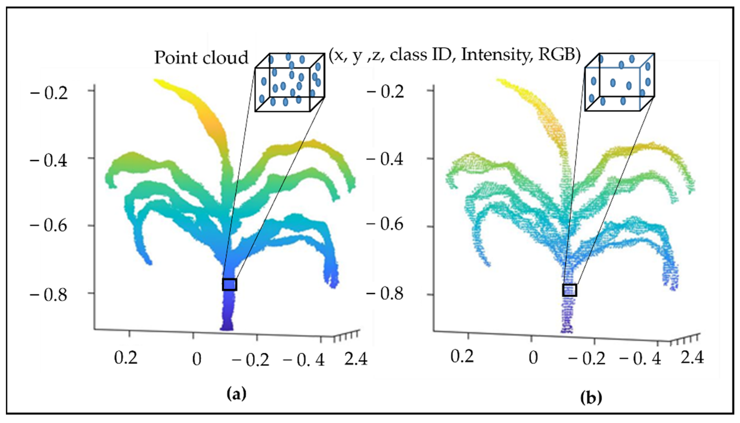
3.3.1. Point Cloud Data Fusion

As we discuss in the previous sections of this article, researchers have proposed and/or deployed many methodologies to perform several operations on spectral images for field crop monitoring. In a similar manner, point cloud data have been adopted for many agricultural applications, such as crop phenotyping analyses [245,246,247,248] and the autonomous navigation of farm tractors and robots in agricultural environments [249,250].

Although we will draw a broader picture, the discipline-specific starting point is the point cloud data model, which is the initial data model common to all multisource fusion methods that include point clouds. The authors of [251] define the point cloud data model as a set of georeferenced points in 3D Cartesian space that is related to a geospatial reference system (e.g., the Universal Transverse Mercator). We present the visualization of a point cloud and its features in Figure 5. The point features can originate from an active measurement process, such as the LiDAR intensity [252] or they can be derived from postprocessing techniques, such as spectral reconstruction [253].

The end goals of point cloud data fusion are to utilize the 3D geometric, spatial structural, and lidar backscatter information inherent in point clouds and fuse it with spectral data sources, or in some cases, geoinformation layers, such as geographic information system (GIS) data. We can generally categorize the methodological approaches to point cloud data fusion in the literature into three main concepts: (1) the point cloud level, at which the primary point cloud is enriched with new point features; (2) the image/voxel level, at which new image layers are derived that represent the 3D point cloud information; (3) the feature level, at which the point cloud information is fused on the segment/object level [240]. The choice of method is largely dependent on the target model after the data fusion. For example, the classification of a dataset calls for point cloud or image level processing.

The concept of enriching the point cloud with features (also known as point cloud coregistration or alignment) involves texturing the point clouds with the image data, usually from either a multisensor system, such as lidar systems mounted with spectral cam-eras, or from photogrammetric point clouds (i.e., the structure from motion and dense image matching). Under this, precise coregistration is used to transfer the labels of the classified spectral data to the corresponding 3D points. With this approach, the authors of [254] related the spectra from 2D multispectral aerial imagery and thermal imagery to 3D point cloud crop models to classify vines in different vigor classes. According to their results, the discriminant power of single indices can be increased and enhanced by their combination, with the best performance obtained using the whole set.

Unlike the point cloud level methodological concept, the image/voxel level is con-cerned with the transformation of point clouds into 2D images or voxels that can be ana-lyzed by the image-processing approaches discussed in Section 3.2 of this article. We can directly derive a number of 2D images from the rich point clouds that come from the point cloud geometry, lidar backscatter, and full-waveform lidar data. Finally, the feature/object level concept is based on the first two concepts in terms of the data model, which is used to derive objects, followed by a classification step. We can use approaches such as image or point cloud segmentation to derive the attributes for the classification.

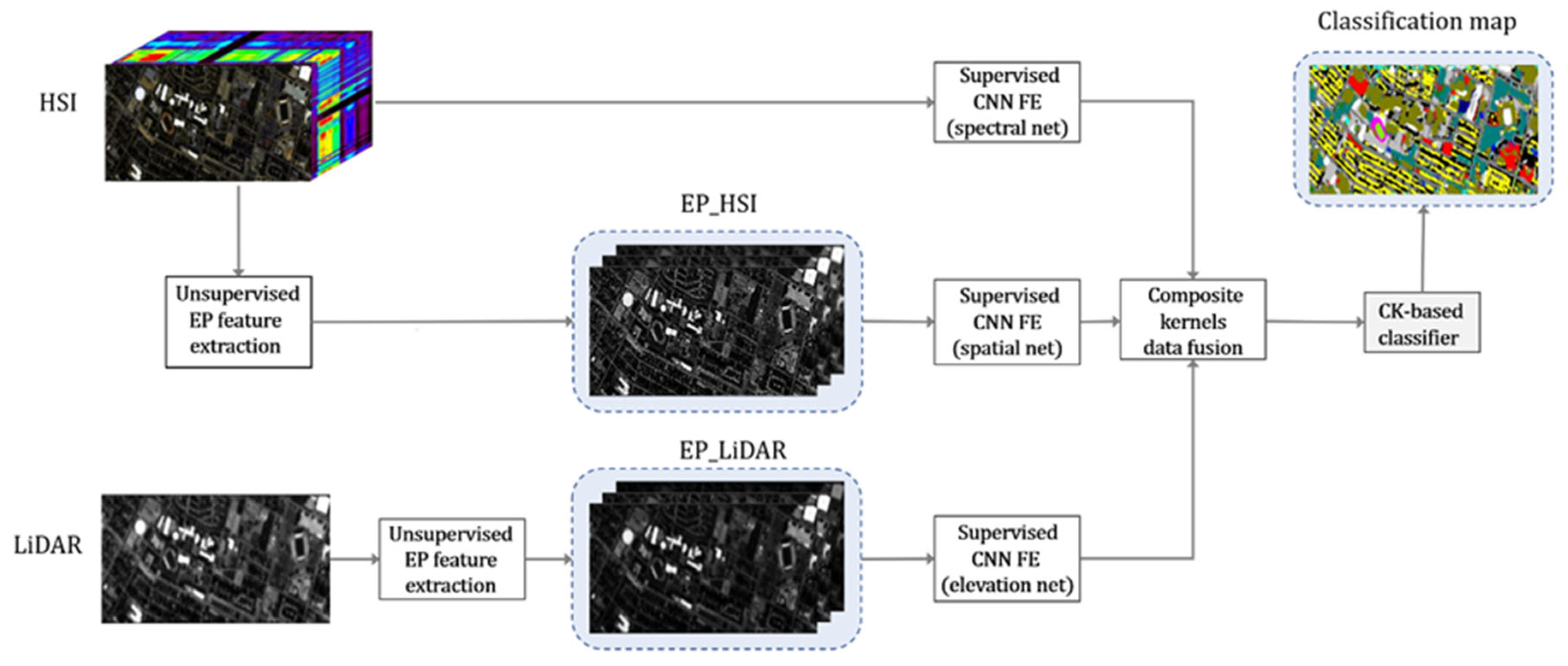
Hyperspectral and LiDAR Data Fusion

HSI technology has certain limitations in terms of differentiating between objects that are composed of the same spectral characteristics (e.g., the same crop species under the same health conditions). In the same way, LiDAR point cloud data alone cannot differentiate between objects in absolute proximity and of the same size, shape, and elevation (e.g., the Eleusineindica species in a finger millet field) due to the lack of spectral information pro-vided by these sensors.

Advancements in multisensor data fusion to take advantage of the information pro-vided by the different sensors that simultaneously capture a particular scene provide potential solutions to the abovementioned issues [255]. Researchers have developed many computer vision algorithms to implement such a solution, including machine-learning and deep-learning algorithms. For HSI and LiDAR data fusion, we can broadly categorize the available techniques in the literature into three major categories: data association, state estimation, and decision fusion [242].

The aim of data association (also known as pixel-level fusion) is to improve the quality via the fusion of the oriented observation data. State estimation (also called feature-level fusion) is carried out by extracting features from different data sources to create new features or feature vectors, which are usually adopted to facilitate the subsequent application. Decision-level fusion inputs different sensor data to separately interpret the land-cover features and obtain the land-cover feature categories, and it then applies certain decision rules to fuse them. As there is typically a large gap in the imaging patterns between different sensors, the most commonly implemented fusion strategy for HSI and LiDAR fusion is feature-level fusion [256]; however, more recently, researchers have combined feature-level fusion with decision fusion to improve the fusion accuracy. Furthermore, they have widely applied CNN architectures in HSI and LiDAR fusion due to their robust feature representation abilities and ability to naturally adapt to images [256]. As there is a considerably large number of publications in the literature regarding data fusion, including the basic steps involved, we do not intend to review all the studies in this section. Instead, we aim to highlight studies in which the authors used the most recent techniques for hyperspectral and LiDAR data fusion. In particular, we explore the methods that use convolutional neural network (CNN) architectures in detail, considering that they are more powerful than conventional techniques for supervised inference tasks [256].

Li [257] proposed a CNN and composite kernel-based novel framework for the fusion of hyper-spectral images and LiDAR-derived elevation data (Figure 6). They took advantage of a combination of extinction profiles (first proposed for use in remote sensing data processing by Ghamisi et al. [258]; this is a technique-based extinction filter using extrema-oriented connected independent filters) and CNN features to enable the joint use of low- and high-level features to improve the classification performance. They initially applied extinction profiles to both data sources to extract the spatial and elevation features from hyperspectral and Li-DAR-derived data, respectively. Next, they designed a three-stream CNN to independently extract the useful spectral, spatial, and elevation features from both data sources. Instead of a simple stacking strategy, as first proposed in [241,259], they again designed a multisensor composite kernel (MCK) scheme to fuse the heterogeneous spectral, spatial, and elevation features extracted by the CNN. This scheme resulted in the higher spectral, spatial, and elevation separability of the extracted features, which enabled them to effectively perform multisensor data fusion in the kernel space.

The simple stacking strategy proposed in [241,259] requires a fully connected layer to fuse the feature extracts; however, fully connected layers often contain a substantially large number of parameters, which increases the training difficulty when considering a small number of training samples. Support vector machines and extreme-learning machines, with their composite kernel versions, were the two machine-learning classifiers employed to produce the final classification result. The concept of the kernel method here refers to using a nonlinear mapping function (e.g., Hilbert kernel) to transfer the input data from the original feature space into a higher feature space, such that the nonlinear problem in the feature space can be transformed into a linear problem. Furthermore, the theoretical elegance of the kernel trick makes it an effective tool for HSI analysis due to its insensitivity to the Hughes phenomenon (also referred to as the curse of dimensionality).

The researchers applied the proposed framework on two commonly used public datasets with different characteristics: an urban data set captured over Houston, the United States, and a rural dataset captured over Trento, Italy. The framework yielded high overall accuracies of 92.57% and 97.91% for the Houston and Trento datasets, respectively. Moreover, according to the authors, the proposed fusion framework can be regarded as a general data fusion framework that can be applied to any other dataset containing both hyperspectral and LiDAR data. They particularly highlight its use in agricultural data to better classify certain classes (e.g., healthy or stressed crops).

Ge et al. [260] extended the work of Ghamisi [257] by proposing a residual fusion strategy that combines the extinction profile (EP) extraction method with the local binary pattern (LBP) method to improve the accuracy and reliability of the feature extraction. They fed the combined output of the two feature extraction strategies into a kernel collaborative representation-based classifier with Tikhonov regularization (KCRT), which Li et al. [261] demonstrated as superior to collaborative representation-based classification (CRC), first proposed by Wang et al. [262], which is because the regularization term in the original CRC could not be adaptively adjusted according to the similarity between the training and testing samples.

Later on, Xia et al. [263] proposed another approach: semisupervised graph fusion (SSGF). Particularly, they introduced the unsupervised fusion graph into the semisupervised local discriminant analysis (SELD) framework proposed by the authors of [264,265] to learn the projection matrix. They first applied morphological filters to LiDAR data and the first few components of the hyperspectral data to model their respective heights and spatial information. Then, they used the proposed SSGF algorithm to generate the spectral, elevation, and spatial features in a lower subspace to obtain the new features. The objective of SSGF is to maximize the class separation ability and preserve the local neighborhood structure by using both labeled and unlabeled samples.

Although the CNN-based approaches have produced excellent performance measures up to this point, compared with conventional techniques, the main disadvantage of this approach is that the feature extraction of different data sources is individually performed, instead of jointly, exploiting the features from both modalities. According to Mohla [266], this results in the loss of some important shared high-level features from both modalities. Furthermore, Chen [267] earlier argued that such an approach may create a substantial imbalance among the different features, which can lead to inequality in the represented information. For this reason, a few researchers have attempted to address this issue.

Wang et al. [268] proposed a novel multiattentive hierarchical fusion net (MAHiDFNet) to achieve the feature-level fusion and classification of HSI and LiDAR data. Particularly, they first developed a three-branch HSI–LiDAR CNN backbone, similar to that in [257], to simultaneously extract the spatial, spectral, and elevation features of the land-cover objects. Mohla [266] first proposed this simultaneous feature extraction during HSI–LiDAR data fusion for use in the context of land-cover classification. The researchers fused the oriented feature embedding by applying a hierarchical fusion strategy based on the output of the triple-branch CNN. Then, they adopted an attention-module-based shallow feature fusion strategy to highlight the modality-specific and modality-integrated features. To construct the hierarchical feature fusion framework in the deep feature fusion stage, they fused the acquired multimodality features, and they finally fed the fused features into the classification module to obtain the classification result at the pixel level.

In summary, there have been substantial efforts made towards finding effective ways to deal with the large data that are currently being captured in agricultural environments. Despite these efforts, data and analysis gaps are still prevalent due to the fact that agricultural environments are mostly uncontrolled and there are a vast number of factors that need to be considered and properly measured for the full characterization of a given area. According to Silveira [269], one of these factors concerns the complexity that is associated with agricultural environments. For example, the information that is captured is not sufficient to cover all the variations found in real practice. The information captured from a single sensor is often incapable of providing explicit solutions, even if the problem at hand is well defined, and effective algorithms are applied. Fusing the information retrieved from different sensors that provide different data types is one possible solution that researchers have explored over the past few years. Data fusion enables the exploration of the complementarities and integration of different data types to obtain more reliable and useful information on the areas of analysis. Whereas some success has been achieved, as discussed in this section, there are still a number of challenges that hinder the more extensive adoption of this type of approach, and especially for agricultural areas with highly complex environments [270].

3.3.2. Spatiotemporal Fusion

As the size of the region-of-interest (ROI) continues to increase, such as in remote sensing at the regional and global scales, there is a tradeoff between the spatial resolution and temporal resolution (i.e., the temporal revisit frequency). As an example, NASA’s Moderate-Resolution Imaging Spectroradiometer (MODIS) sensor and Aqua satellites collect data at different spatial ranges, from 250 m to 1 km, which are often too coarse to ex-tract the explicit land-cover information that may exist at a finer spatial scale than the sensor resolution. The multispectral onboard Sentinel-2B instrument captures the Earth’s reflected radiance with a high revisit time (i.e., 5 days) and high spatial resolution (four bands at 10 m, six bands at 20 m, and three bands at 60 m) [271]. Thus, due to its low temporal resolution, it is not suitable for monitoring short-term disastrous agricultural events, such as floods.

However, due to recent technical advances, the remote sensing community now has access to both dense timeseries data and high spatial- and spectral-resolution images. For example, Sentinel-3 Ocean and the Land Color Imager (OLCI) sensor currently provide images at a spatial resolution of 300 m and a temporal resolution of 2.8 days, which are expected to increase upon the launch of Sentinel-3B. Moreover, Planet’s microsatellites acquire daily images at a spatial resolution of 3.125 m. Likewise, for relatively manageable small-scale applications, the recent advancements in remotely piloted aircraft systems, or drones, provide a considerable amount of multisource data with high spatial and temporal resolutions. However, these studies require access to historical data, which have fine temporal and spatial resolutions.

The authors of [271,272], along with those of other articles in the literature, provide in-depth well-established discussions and/or implementations of several spatiotemporal data fusion methods and techniques based on remote satellites. In the context of satellite remote sensing, spatiotemporal fusion can be performed either by combining low- and high-spatial resolution imagery from the same satellite system (e.g., 30 m multispectral imagery with 15 m pan-chromatic images from the Landsat satellite), or from different satellite systems [273]. Researchers have developed several methods to achieve spatiotemporal fusion across different application fields, such as crop and urban growth monitoring. According to [274], we can broadly classify these methods into three major groups: (1) reconstruction-based methods; (2) learning-based methods; and (3) unmixing-based methods. However, the authors of [272] argue that these three broad categories are not sufficient to cover all the spatiotemporal fusion methods. Therefore, they propose five categories based on the specific techniques used to link fine and coarse images: (1) unmixing-based methods; (2) weight-function-based methods; (3) Bayesian-based methods; (4) learning-based methods; and (5) hybrid methods.

Spectral unmixing-based methods approximate the fine pixel values by unmixing the coarse pixels based on the theory of linear spectral mixtures to extract the endmembers and abundances (i.e., the proportions at the subpixel level) [275]. High-resolution datasets provide a number of endmembers and abundances obtained from a, and the spectral signature of the endmembers is unmixed from the coarse-resolution dataset. The assumption behind linear spectral mixing theory is that the reflectance that corresponds to each coarse spatial-resolution pixel is a linear combination of the responses of each land-cover class that contributes to the mixture [276]. The four steps in spectral unmixing required to predict a fine-resolution image are as follows: (1) the classification of the image with high spatial resolution using unsupervised methods, such as k-means; (2) the computation of the endmember fractions of each coarse pixel; (3) the unmixing of the coarse pixels at the prediction date within a moving window; and (4) the assignment of the unmixed reflectance to fine pixels.

Learning-based methods take advantage of the intrinsic capabilities of machine learning to predict the unobserved finer-temporal-resolution images from coarse-spatial-resolution images. The most commonly employed machine-learning methods for spatiotemporal data fusion include regression trees [277], random forest [278], dictionary-pair learning [279], extreme learning [280], artificial neural networks [281] and convolutional neural networks [280].

Bayesian-based methods, as the name suggests, use the Bayesian probabilistic theory of estimation to combine images. Under this framework, the goal of data fusion is to achieve the desired fine image at the prediction date by maximizing its conditional prob-ability relative to the fine and coarse input images [282]. In other words, Bayesian-based data fusion aims to discover how to model two relationships (i.e., between the observed coarse image and fine image observed at the same date and the one observed at different dates) between the input images and predicted image.

Researchers use weighted-function-based methods, which are also called reconstruction-based methods [271], to estimate the synthetic spectral reflectance at the pixel level by means of the weighted sum of the similar neighboring pixels of the input image source. Researchers have developed many methods under the weighted-function-based approach, which, among others, include the following: the spatial and temporal adaptive reflectance fusion model (STARFM) [283]; enhanced STARFM semiphysical fusion approach [284]; spatiotemporal adaptive data fusion algorithm for temperature mapping (SADFAT) [255]; spatial temporal adaptive algorithm for mapping reflectance change (STAARCH) [285]; spatiotemporal integrated temperature fusion model (STITFM) [274]; spatiotemporal enhancement method for medium-resolution LAI (STEM-LAI) [286]; spatiotemporal vegetation index image fusion model (STVIFM) [287]; and database unmixing (DBUX) [288]. Among these methods, the most applied reconstruction-based image fusion method is the STARFM [271] due to its ability to accurately predict the surface reflectance on a daily basis at an effective resolution that is close to that of the Landsat enhanced thematic mapper Plus (ETM+) (i.e., 30 m). However, its performance largely depends on the characteristic patch size of the landscape and reduces to some extent when used on landscapes with extremely heterogeneous fine grains.

The integration of two or more of the four abovementioned categories constitutes the fifth category: hybrid methods, the purpose of which is to improve the spatiotemporal da-ta fusion performance through the utilization of the advantages associated with the individual methods. One of the recently developed hybrid methods is flexible spatiotemporal data fusion (FSDAF), which combines weighted-function-based methods and unmixing-based methods [289], which makes it effective even in highly heterogenous landscapes. Other hybrid methods in the literature include the spatial and temporal reflectance unmixing model (STRUM) [275], and the spatial–temporal remotely sensed images and land-cover maps fusion model (STIMFM) [290].

3.3.3. Spatiospectral Fusion

Similarly, as is the case for spatiotemporal fusion, different satellite sensors can be used to observe the surface of the Earth at different spatial resolutions over a given wave-length range. For instance, Planet microsatellites acquire multispectral images at a spatial resolution of 3.125 m, and a single single-band panchromatic (PAN) image has a spatial resolution of 0.73 m (SkySat-3 and SkySat-14), whereas the multispectral instrument onboard Sentinel-2B captures the Earth’s reflected radiance with a lower spatial resolution (four bands at 10 m, six bands at 20 m, and three bands at 60 m). Therefore, the aim of spatiospectral fusion is to combine fine-resolution and coarse-resolution images (e.g., 3.125 m SkySat-3 multispectral images and 0.73 m SkySat-3 PAN images) to derive fi-ne-spatial-resolution images for all the bands. The use of only a single PAN image as the fine-resolution image is referred to as “pan-sharpening” (the example given above for SkySat-3), whereas the use of multiple fine images is referred to as multiband image fusion (e.g., fusing the different resolution bands of Sentinel-2B).

Over time, researchers have developed many techniques to perform spatiospectral fusion, which they have broadly divided into five categories: (1) multiresolution analysis (MRA); (2) component substitution (CS); (3) geostatistical analysis; (4) subspace representation; (5) sparse representation [240]

CS [291] was developed in 1987 to merge multiresolution SPOT HRV and Landsat TM data, and it was designed to spectrally transform the multispectral data into a different feature space to separate the spatial and spectral information into different components. PCA [292] is one of the most applied methods for transformation. Other methods include Gram–Schmidt [293] and hue saturation [294], among others. In these approaches, the component that contains the spatial information is replaced with the panchromatic image for the transformation into the sharpened image.

After the CS approach, researchers continued to propose different techniques with intrinsic advantages, such as multiresolution analysis [295], the main advantage of which is the spectral consistency, such that if the combined image is degraded in the spatial domain, then the degraded image is spectrally consistent with the input coarse-spatial-resolution and fine-spectral-resolution image [240]. Researchers have also developed geostatistical analysis to preserve the spectral properties of the original coarse images so that, when the downscaled image is upscaled to the original coarse spatial resolution, the obtained result is identical to the original one [296]. Subspace representation is a technique that approaches the spatiospectral fusion problem through the spectral characteristic analysis of the scene of interest using a subspace that is spanned by a set of basis vectors, such as the principal component bases and spectral signatures of endmembers [297]. Recently, the authors of [298] proposed another approach, sparse representation, which is based on patch-wise sparse representation to exploit the various external fine-spatial-resolution multispectral images as the database.

Pedram et al. [240] present a detailed comparative review of these approaches, with a statistical analysis of the history and annual average number of citations for each category of the abovementioned spatiospectral techniques. According to their research, the most applied techniques in the last two decades have been component substitution and multiresolution analysis. In recent years, the remaining three approaches have achieved considerable applications due to their simplicity, outperforming the previous approaches.

Moreover, the use of hyperspectral imaging and data fusion techniques is becoming more and more important in almost all environmental and agricultural related aspects indifferent from field crop monitoring. For instance, there has been a lot more ongoing studies on monitoring the recovery of abandoned industrial areas through the recovery of land with woods or agricultural areas in some cases. A recent study by Giuseppe et al. [299] shows the potential to identify and characterize areas contaminated by asbestos in a mining site using remote sensing techniques coupled with data fusion based on the PRISMA satellite hyperspectral images.

4. Conclusions

According to our review, the advent of remote sensing has substantially fueled the success of precision agriculture in response to the rapidly growing global food demand amidst the effects of climate change. Spectral imaging has played a vital role in facilitating crop monitoring to aid the decision making in the implementation of spatially variable agronomic practices and/or inputs. Driven by cutting-edge data processing techniques, spectral imaging for field crop monitoring has become a prominent research area in the remote sensing community. Furthermore, the recent data fusion approaches have eliminated the need to compromise between the spatial and spectral resolutions. Due to recent technical advances, the remote sensing community now has access to both dense timeseries data and high-spatiospectral-resolution images, without the need to approximate the compromised components using fusion methods. Moreover, machine-learning and deep-learning approaches have substantially enhanced the processing and analysis of spectral information. However, in these approaches, it is assumed that there are sufficient computational resources, and that no data transmission cost is incurred for their optimal application; however, this is not always the case.

References

1. FAO. 2017 The State of Food and Agrivulture Leveraging Food Systems for Inclusive Rural Transformation; Food & Agriculture Organization: Roam, Italy, 2017; ISBN 9789251098738. [Google Scholar]
2. Sishodia, R.P.; Ray, R.L.; Singh, S.K. Applications of Remote Sensing in Precision Agriculture: A Review. Remote Sens. 2020, 12, 3136. [Google Scholar] [CrossRef]
3. Morison, J.I.L.; Matthews, R.B. Agriculture and Forestry Climate Change Impacts Summary Report, Living With Environmental Change. In Living With Environmental Change; Living With Environmental Change: London, UK, 2016. [Google Scholar]
4. Eugen, L. Technology Executive Committee Ninth meeting of the Technology Executive Committee TEC Brief on technologies for Adaptation-Water. Available online: www.ipcc-wg2.gov/AR5 (accessed on 14 October 2022).
5. Gassner, A.; Coe, R.; Sinclair, F. Improving food security through increasing the precision of agricultural development. In Precision Agriculture for Sustainability and Environmental Protection; Taylor & Francis: London, UK, 2013. [Google Scholar] [CrossRef]
6. Morisse, M.; Wells, D.M.; Millet, E.J.; Lillemo, M.; Fahrner, S.; Cellini, F.; Lootens, P.; Muller, O.; Herrera, J.M.; Bentley, A.R.; et al. A European perspective on opportunities and demands for field-based crop phenotyping. Field Crop. Res. 2022, 276, 108371. [Google Scholar] [CrossRef]
7. Hagen, N.; Kudenov, M.W. Review of snapshot spectral imaging technologies. Opt. Eng. 2013, 52, 090901. [Google Scholar] [CrossRef] [Green Version]
8. Liu, N.; Townsend, P.A.; Naber, M.R.; Bethke, P.C.; Hills, W.B.; Wang, Y. Hyperspectral imagery to monitor crop nutrient status within and across growing seasons. Remote Sens. Environ. 2021, 255, 112303. [Google Scholar] [CrossRef]
9. Qin, J.; Chao, K.; Kim, M.S.; Lu, R.; Burks, T.F. Hyperspectral and multispectral imaging for evaluating food safety and quality. J. Food Eng. 2013, 118, 157–171. [Google Scholar] [CrossRef]
10. Yang, G.; Liu, J.; Zhao, C.; Li, Z.; Huang, Y.; Yu, H.; Xu, B.; Yang, X.; Zhu, D.; Zhang, X.; et al. Unmanned aerial vehicle remote sensing for field-based crop phenotyping: Current status and perspectives. Front. Plant Sci. 2017, 8, 1111. [Google Scholar] [CrossRef] [Green Version]
11. Kundu, R.; Dutta, D.; Nanda, M.K.; Chakrabarty, A. Near Real Time Monitoring of Potato Late Blight Disease Severity using Field Based Hyperspectral Observation. Smart Agric. Technol. 2021, 1, 100019. [Google Scholar] [CrossRef]
12. Elgendy, N.; Elragal, A.; Päivärinta, T. DECAS: A modern data-driven decision theory for big data and analytics. J. Decis. Syst. 2022, 31, 337–373. [Google Scholar] [CrossRef]
13. Aviara, N.A.; Liberty, J.T.; Olatunbosun, O.S.; Shoyombo, H.A.; Oyeniyi, S.K. Potential application of hyperspectral imaging in food grain quality inspection, evaluation and control during bulk storage. J. Agric. Food Res. 2022, 8, 100288. [Google Scholar] [CrossRef]
14. Pieczywek, P.M.; Cybulska, J.; Szymańska-Chargot, M.; Siedliska, A.; Zdunek, A.; Nosalewicz, A.; Baranowski, P.; Kurenda, A. Early detection of fungal infection of stored apple fruit with optical sensors–Comparison of biospeckle, hyperspectral imaging and chlorophyll fluorescence. Food Control 2018, 85, 327–338. [Google Scholar] [CrossRef]
15. Li, J.; Sun, D.; Cheng, J. Recent advances in nondestructive analytical techniques for determining the total soluble solids in fruits: A review. Compr. Rev. Food Sci. Food Saf. 2016, 15, 897–911. [Google Scholar] [CrossRef]
16. Erkinbaev, C.; Henderson, K.; Paliwal, J. Discrimination of gluten-free oats from contaminants using near infrared hyperspectral imaging technique. Food Control 2017, 80, 197–203. [Google Scholar] [CrossRef]
17. Fox, G.; Manley, M. Applications of single kernel conventional and hyperspectral imaging near infrared spectroscopy in cereals. J. Sci. Food Agric. 2014, 94, 174–179. [Google Scholar] [CrossRef]
18. Orina, I.; Manley, M.; Williams, P.J. Non-destructive techniques for the detection of fungal infection in cereal grains. Food Res. Int. 2017, 100, 74–86. [Google Scholar] [CrossRef]
19. Kandpal, L.M.; Lee, S.; Kim, M.S.; Bae, H.; Cho, B.-K. Short wave infrared (SWIR) hyperspectral imaging technique for examination of aflatoxin B1 (AFB1) on corn kernels. Food Control 2015, 51, 171–176. [Google Scholar] [CrossRef]
20. Hussain, N.; Sun, D.-W.; Pu, H. Classical and emerging non-destructive technologies for safety and quality evaluation of cereals: A review of recent applications. Trends Food Sci. Technol. 2019, 91, 598–608. [Google Scholar] [CrossRef]
21. Wójtowicz, M.; Wójtowicz, A.; Piekarczyk, J. Application of remote sensing methods in agriculture. Commun. Biometry Crop Sci. 2016, 11, 31–50. [Google Scholar]
22. Khorram, S.; van der Wiele, C.F.; Koch, F.H.; Nelson, S.A.C.; Potts, M.D. Principles of Applied Remote Sensing; Springer: Cham, Switzerland, 2016; ISBN 9783319225609. [Google Scholar]
23. Sankaran, S.; Ehsani, R. Introduction to the electromagnetic spectrum. In Imaging with Electromagnetic Spectrum; Springer: Berlin/Heidelberg, Germany, 2014; pp. 1–15. [Google Scholar]
24. Strati, V.; Albéri, M.; Anconelli, S.; Baldoncini, M.; Bittelli, M.; Bottardi, C.; Chiarelli, E.; Fabbri, B.; Guidi, V.; Raptis, K.G.C. Modelling soil water content in a tomato field: Proximal gamma ray spectroscopy and soil–crop system models. Agriculture 2018, 8, 60. [Google Scholar] [CrossRef] [Green Version]
25. Mahmood, H.S.; Hoogmoed, W.B.; Van Henten, E.J. Proximal gamma-ray spectroscopy to predict soil properties using windows and full-spectrum analysis methods. Sensors 2013, 13, 16263–16280. [Google Scholar] [CrossRef] [Green Version]
26. de Castilhos, N.D.B.; Melquiades, F.L.; Thomaz, E.L.; Bastos, R.O. X-ray fluorescence and gamma-ray spectrometry combined with multivariate analysis for topographic studies in agricultural soil. Appl. Radiat. Isot. 2015, 95, 63–71. [Google Scholar] [CrossRef]
27. Mukhopadhyay, S.; Chakraborty, S.; Bhadoria, P.B.S.; Li, B.; Weindorf, D.C. Assessment of heavy metal and soil organic carbon by portable X-ray fluorescence spectrometry and NixProTM sensor in landfill soils of India. Geoderma Reg. 2020, 20, e00249. [Google Scholar] [CrossRef]
28. Wan, M.; Hu, W.; Qu, M.; Tian, K.; Zhang, H.; Wang, Y.; Huang, B. Application of arc emission spectrometry and portable X-ray fluorescence spectrometry to rapid risk assessment of heavy metals in agricultural soils. Ecol. Indic. 2019, 101, 583–594. [Google Scholar] [CrossRef]
29. Antenozio, M.L.; Capobianco, G.; Costantino, P.; Vamerali, T.; Bonifazi, G.; Serranti, S.; Brunetti, P.; Cardarelli, M. Arsenic accumulation in Pteris vittata: Time course, distribution, and arsenic-related gene expression in fronds and whole plantlets. Environ. Pollut. 2022, 309, 119773. [Google Scholar] [CrossRef] [PubMed]
30. Arsego, F.; Ware, A.; Oakey, H. Proximal sensing technologies on soils and plants on Eyre Peninsula. In Proceedings of the 2019 Agronomy Australia Conference, Wagga Wagga, Australia, 25–29 August 2019. [Google Scholar]
31. Manickavasagan, A.; Jayasuriya, H. Imaging with Electromagnetic Spectrum: Applications in Food and Agriculture; Springer: Berlin/Heidelberg, Germany, 2014; ISBN 3642548881. [Google Scholar]
32. Zhao, T.; Nakano, A. Agricultural Product Authenticity and Geographical Origin Traceability-Use of Nondestructive Measurement. Jpn. Agric. Res. Q. JARQ 2018, 52, 115–122. [Google Scholar] [CrossRef] [Green Version]
33. Patel, K.K.; Kar, A.; Khan, M.A. Potential of reflected UV imaging technique for detection of defects on the surface area of mango. J. Food Sci. Technol. 2019, 56, 1295–1301. [Google Scholar] [CrossRef]
34. Sankaran, S.; Ehsani, R.; Etxeberria, E. Mid-infrared spectroscopy for detection of Huanglongbing (greening) in citrus leaves. Talanta 2010, 83, 574–581. [Google Scholar] [CrossRef]
35. Mousa, M.A.A.; Wang, Y.; Antora, S.A.; Al-Qurashi, A.D.; Ibrahim, O.H.M.; He, H.-J.; Liu, S.; Kamruzzaman, M. An overview of recent advances and applications of FT-IR spectroscopy for quality, authenticity, and adulteration detection in edible oils. Crit. Rev. Food Sci. Nutr. 2022, 62, 8009–8027. [Google Scholar] [CrossRef]
36. El Fakir, C.; Hjeij, M.; Le Page, R.; Poffo, L.; Billiot, B.; Besnard, P.; Goujon, J.-M. Active hyperspectral mid-infrared imaging based on a widely tunable quantum cascade laser for early detection of plant water stress. Opt. Eng. 2021, 60, 23106. [Google Scholar] [CrossRef]
37. Shen, Y.; Wu, X.; Wu, B.; Tan, Y.; Liu, J. Qualitative analysis of lambda-cyhalothrin on Chinese cabbage using mid-infrared spectroscopy combined with fuzzy feature extraction algorithms. Agriculture 2021, 11, 275. [Google Scholar] [CrossRef]
38. Vanlierde, A.; Dehareng, F.; Gengler, N.; Froidmont, E.; McParland, S.; Kreuzer, M.; Bell, M.; Lund, P.; Martin, C.; Kuhla, B. Improving robustness and accuracy of predicted daily methane emissions of dairy cows using milk mid-infrared spectra. J. Sci. Food Agric. 2021, 101, 3394–3403. [Google Scholar] [CrossRef]
39. Rai, M.; Maity, T.; Yadav, R.K. Thermal imaging system and its real time applications: A survey. J. Eng. Technol. 2017, 6, 290–303. [Google Scholar]
40. Roopaei, M.; Rad, P.; Choo, K.-K.R. Cloud of Things in Smart Agriculture: Intelligent Irrigation Monitoring by Thermal Imaging. IEEE Cloud Comput. 2017, 4, 10–15. [Google Scholar] [CrossRef]
41. Das, S.; Chapman, S.; Christopher, J.; Choudhury, M.R.; Menzies, N.W.; Apan, A.; Dang, Y.P. UAV-thermal imaging: A technological breakthrough for monitoring and quantifying crop abiotic stress to help sustain productivity on sodic soils—A case review on wheat. Remote Sens. Appl. Soc. Environ. 2021, 23, 100583. [Google Scholar] [CrossRef]
42. Cohen, B.; Edan, Y.; Levi, A.; Alchanatis, V. Early detection of grapevine downy mildew using thermal imaging. In Precision Agriculture ’21; Wageningen Academic Publishers: Wageningen, The Netherlands, 2021; pp. 283–290. [Google Scholar]
43. Mokari, E.; Samani, Z.; Heerema, R.; Dehghan-Niri, E.; DuBois, D.; Ward, F.; Pierce, C. Development of a new UAV-thermal imaging based model for estimating pecan evapotranspiration. Comput. Electron. Agric. 2022, 194, 106752. [Google Scholar] [CrossRef]
44. Pastorino, M.; Randazzo, A. Microwave Imaging Methods and Applications; Artech House: New York, NY, USA, 2018; ISBN 9781630815264. [Google Scholar]
45. Ghavami, N.; Sotiriou, I.; Kosmas, P. Experimental investigation of microwave imaging as means to assess fruit quality. In Proceedings of the 2019 13th European Conference on Antennas and Propagation (EuCAP), Krakow, Poland, 31 March–5 April 2019; pp. 1–5. [Google Scholar]
46. Saeidi, T.; Ismail, I.; Mahmood, S.N.; Alani, S.; Alhawari, A.R.H. Microwave Imaging of Voids in Oil Palm Trunk Applying UWB Antenna and Robust Time-Reversal Algorithm. J. Sens. 2020, 2020, 8895737. [Google Scholar] [CrossRef]
47. Shi, X.; Li, J.; Mukherjee, S.; Datta, S.; Rathod, V.; Wang, X.; Lu, W.; Udpa, L.; Deng, Y. Ultra-Wideband Microwave Imaging System for Root Phenotyping. Sensors 2022, 22, 2031. [Google Scholar] [CrossRef]
48. Pallav, P.; Hutchins, D.A.; Gan, T. Air-coupled ultrasonic evaluation of food materials. Ultrasonics 2009, 49, 244–253. [Google Scholar] [CrossRef]
49. Ok, G.; Choi, S.-W.; Park, K.H.; Chun, H.S. Foreign object detection by sub-terahertz quasi-Bessel beam imaging. Sensors 2012, 13, 71–85. [Google Scholar] [CrossRef] [Green Version]
50. Jafarbiglu, H.; Pourreza, A. A comprehensive review of remote sensing platforms, sensors, and applications in nut crops. Comput. Electron. Agric. 2022, 197, 106844. [Google Scholar] [CrossRef]
51. Walter, V.; Saska, M.; Franchi, A. Fast mutual relative localization of uavs using ultraviolet led markers. In Proceedings of the 2018 International Conference on Unmanned Aircraft Systems (ICUAS), Dallas, TX, USA, 12–15 June 2018; pp. 1217–1226. [Google Scholar]
52. Xu, J.; Mishra, P. Combining deep learning with chemometrics when it is really needed: A case of real time object detection and spectral model application for spectral image processing. Anal. Chim. Acta 2022, 1202, 339668. [Google Scholar] [CrossRef]
53. Nicolis, O.; Gonzalez, C. Wavelet-based fractal and multifractal analysis for detecting mineral deposits using multispectral images taken by drones. Methods Appl. Pet. Miner. Explor. Eng. Geol. 2021, 295–307. [Google Scholar] [CrossRef]
54. Drusch, M.; Del Bello, U.; Carlier, S.; Colin, O.; Fernandez, V.; Gascon, F.; Hoersch, B.; Isola, C.; Laberinti, P.; Martimort, P. Sentinel-2: ESA’s optical high-resolution mission for GMES operational services. Remote Sens. Environ. 2012, 120, 25–36. [Google Scholar] [CrossRef]
55. Jin, X.; Li, Z.; Feng, H.; Ren, Z.; Li, S. Deep neural network algorithm for estimating maize biomass based on simulated Sentinel 2A vegetation indices and leaf area index. Crop J. 2020, 8, 87–97. [Google Scholar] [CrossRef]
56. Yue, J.; Yang, G.; Tian, Q.; Feng, H.; Xu, K.; Zhou, C. Estimate of winter-wheat above-ground biomass based on UAV ultrahigh-ground-resolution image textures and vegetation indices. ISPRS J. Photogramm. Remote Sens. 2019, 150, 226–244. [Google Scholar] [CrossRef]
57. Han, L.; Yang, G.; Dai, H.; Xu, B.; Yang, H.; Feng, H.; Li, Z.; Yang, X. Modeling maize above-ground biomass based on machine learning approaches using UAV remote-sensing data. Plant Methods 2019, 15, 1–19. [Google Scholar] [CrossRef] [Green Version]
58. Li, W.; Jiang, J.; Weiss, M.; Madec, S.; Tison, F.; Philippe, B.; Comar, A.; Baret, F. Impact of the reproductive organs on crop BRDF as observed from a UAV. Remote Sens. Environ. 2021, 259, 112433. [Google Scholar] [CrossRef]
59. Pereira, F.R.; de Lima, J.P.; Freitas, R.G.; Dos Reis, A.A.; do Amaral, L.R.; Figueiredo, G.K.D.A.; Lamparelli, R.A.C.; Magalhães, P.S.G. Nitrogen variability assessment of pasture fields under an integrated crop-livestock system using UAV, PlanetScope, and Sentinel-2 data. Comput. Electron. Agric. 2022, 193, 106645. [Google Scholar] [CrossRef]
60. ElMasry, G.; Mandour, N.; Al-Rejaie, S.; Belin, E.; Rousseau, D. Recent applications of multispectral imaging in seed phenotyping and quality monitoring—An overview. Sensors 2019, 19, 1090. [Google Scholar] [CrossRef] [Green Version]
61. Hossen, M.A.; Diwakar, P.K.; Ragi, S. Total nitrogen estimation in agricultural soils via aerial multispectral imaging and LIBS. Sci. Rep. 2021, 11, 12693. [Google Scholar] [CrossRef]
62. Qi, H.; Wu, Z.; Zhang, L.; Li, J.; Zhou, J.; Jun, Z.; Zhu, B. Monitoring of peanut leaves chlorophyll content based on drone-based multispectral image feature extraction. Comput. Electron. Agric. 2021, 187, 106292. [Google Scholar] [CrossRef]
63. Jameel, S.M.; Gilal, A.R.; Rizvi, S.S.H.; Rehman, M.; Hashmani, M.A. Practical implications and challenges of multispectral image analysis. In Proceedings of the 2020 3rd International Conference on Computing, Mathematics and Engineering Technologies (iCoMET), Sukkur, Pakistan, 29–30 January 2020; pp. 1–5. [Google Scholar]
64. Soria, X.; Sappa, A.D.; Akbarinia, A. Multispectral single-sensor RGB-NIR imaging: New challenges and opportunities. In Proceedings of the 2017 Seventh International Conference on Image Processing Theory, Tools and Applications (IPTA), Montreal, QC, Canada, 28 November–1 December 2017; pp. 1–6. [Google Scholar]
65. Dian, R.; Li, S.; Sun, B.; Guo, A. Recent advances and new guidelines on hyperspectral and multispectral image fusion. Inf. Fusion 2021, 69, 40–51. [Google Scholar] [CrossRef]
66. Peón García, J.J.; Fernández Menéndez, S.C.; Recondo González, M.C.; Fernández Calleja, J.J. Evaluation of the spectral characteristics of five hyperspectral and multispectral sensors for soil organic carbon estimation in burned areas. Int. J. Wildl. Fire 2017, 26, 230–239. [Google Scholar] [CrossRef]
67. Castaldi, F.; Palombo, A.; Santini, F.; Pascucci, S.; Pignatti, S.; Casa, R. Evaluation of the potential of the current and forthcoming multispectral and hyperspectral imagers to estimate soil texture and organic carbon. Remote Sens. Environ. 2016, 179, 54–65. [Google Scholar] [CrossRef]
68. Guo, L.; Fu, P.; Shi, T.; Chen, Y.; Zhang, H.; Meng, R.; Wang, S. Mapping field-scale soil organic carbon with unmanned aircraft system-acquired time series multispectral images. Soil Tillage Res. 2020, 196, 104477. [Google Scholar] [CrossRef]
69. Moriya, É.A.S.; Imai, N.N.; Tommaselli, A.M.G.; Berveglieri, A.; Santos, G.H.; Soares, M.A.; Marino, M.; Reis, T.T. Detection and mapping of trees infected with citrus gummosis using UAV hyperspectral data. Comput. Electron. Agric. 2021, 188, 106298. [Google Scholar] [CrossRef]
70. Pandey, P.C.; Balzter, H.; Srivastava, P.K.; Petropoulos, G.P.; Bhattacharya, B. Future perspectives and challenges in hyperspectral remote sensing. Hyperspectral Remote Sens. 2020, 429–439. [Google Scholar] [CrossRef]
71. Goodenough, D.G.; Dyk, A.; Niemann, K.O.; Pearlman, J.S.; Chen, H.; Han, T.; Murdoch, M.; West, C. Processing Hyperion and ALI for forest classification. IEEE Trans. Geosci. Remote Sens. 2003, 41, 1321–1331. [Google Scholar] [CrossRef]
72. Lu, G.; Fei, B. Medical hyperspectral imaging: A review. J. Biomed. Opt. 2014, 19, 10901. [Google Scholar] [CrossRef]
73. Qureshi, R.; Uzair, M.; Zahra, A. Current Advances in Hyperspectral Face Recognition. TechRxiv 2020. [Google Scholar] [CrossRef]
74. Zhang, X.; Zhao, H. Hyperspectral-cube-based mobile face recognition: A comprehensive review. Inf. Fusion 2021, 74, 132–150. [Google Scholar] [CrossRef]
75. Gao, L.; Wang, L.V. A review of snapshot multidimensional optical imaging: Measuring photon tags in parallel. Phys. Rep. 2016, 616, 1–37. [Google Scholar] [CrossRef]
76. Maestro, M.A.; Bañas, A.R.; Lofamia, M.C.; Aguinaldo, R.A.; Bernabe, R.; Occeña, D.J.; Toleos, L.; Madalipay, J.C.; Soriano, M. Development of an airborne hyperspectral scanning camera system for agricultural missions. In Proceedings of the 38th International Communications Satellite Systems Conference (ICSSC 2021), Arlington, VA, USA, 27–30 September 2021; pp. 258–263. [Google Scholar]
77. Davis, S.P.; Abrams, M.C.; Brault, J.W. Fourier Transform Spectrometry; Elsevier: Amsterdam, The Netherlands, 2001; ISBN 0080506917. [Google Scholar]
78. Preda, F.; Perri, A.; Polli, D. A New ‘Hera’in Hyperspectral Imaging: Low light applications come into range thanks to a novel camera system. PhotonicsViews 2021, 18, 45–49. [Google Scholar] [CrossRef]
79. Lohumi, S.; Kim, M.S.; Qin, J.; Cho, B.-K. Raman imaging from microscopy to macroscopy: Quality and safety control of biological materials. TrAC Trends Anal. Chem. 2017, 93, 183–198. [Google Scholar] [CrossRef]
80. Mizuno, T.; Iwata, T. Hadamard-transform fluorescence-lifetime imaging. Opt. Express 2016, 24, 8202–8213. [Google Scholar] [CrossRef] [PubMed] [Green Version]
81. HERA VIS-NIR—Hyperspectral Camera (400–1000 nm). Available online: https://www.nireos.com/hera-visnir/ (accessed on 28 October 2022).
82. Candeo, A.; Nogueira de Faria, B.E.; Erreni, M.; Valentini, G.; Bassi, A.; De Paula, A.M.; Cerullo, G.; Manzoni, C. A hyperspectral microscope based on an ultrastable common-path interferometer. APL Photonics 2019, 4, 120802. [Google Scholar] [CrossRef]
83. Famili, A.; Shen, W.-M.; Weber, R.; Simoudis, E. Data preprocessing and intelligent data analysis. Intell. Data Anal. 1997, 1, 3–23. [Google Scholar] [CrossRef] [Green Version]
84. Wu, D.; Sun, D.-W.; He, Y. Application of long-wave near infrared hyperspectral imaging for measurement of color distribution in salmon fillet. Innov. Food Sci. Emerg. Technol. 2012, 16, 361–372. [Google Scholar] [CrossRef]
85. Williams, P.J.; Geladi, P.; Britz, T.J.; Manley, M. Investigation of fungal development in maize kernels using NIR hyperspectral imaging and multivariate data analysis. J. Cereal Sci. 2012, 55, 272–278. [Google Scholar] [CrossRef]
86. Hughes, G. On the mean accuracy of statistical pattern recognizers. IEEE Trans. Inf. Theory 1968, 14, 55–63. [Google Scholar] [CrossRef] [Green Version]
87. Defernez, M.; Kemsley, E.K. The use and misuse of chemometrics for treating classification problems. TrAC Trends Anal. Chem. 1997, 16, 216–221. [Google Scholar] [CrossRef]
88. Nasibov, H.; Kholmatov, A.; Akselli, B.; Nasibov, A.; Baytaroglu, S. Performance analysis of the CCD pixel binning option in particle-image velocimetry measurements. IEEE/ASME Trans. Mechatron. 2010, 15, 527–540. [Google Scholar] [CrossRef]
89. Mollazade, K.; Omid, M.; Akhlaghian Tab, F.; Rezaei Kalaj, Y.; Mohtasebi, S.S. Data mining-based wavelength selection for monitoring quality of tomato fruit by backscattering and multispectral imaging. Int. J. Food Prop. 2015, 18, 880–896. [Google Scholar] [CrossRef]
90. Jia, B.; Wang, W.; Ni, X.; Lawrence, K.C.; Zhuang, H.; Yoon, S.-C.; Gao, Z. Essential processing methods of hyperspectral images of agricultural and food products. Chemom. Intell. Lab. Syst. 2020, 198, 103936. [Google Scholar] [CrossRef]
91. Yun, Y.-H.; Cao, D.-S.; Tan, M.-L.; Yan, J.; Ren, D.-B.; Xu, Q.-S.; Yu, L.; Liang, Y.-Z. A simple idea on applying large regression coefficient to improve the genetic algorithm-PLS for variable selection in multivariate calibration. Chemom. Intell. Lab. Syst. 2014, 130, 76–83. [Google Scholar] [CrossRef]
92. Senan, E.M.; Abunadi, I.; Jadhav, M.E.; Fati, S.M. Score and Correlation Coefficient-Based Feature Selection for Predicting Heart Failure Diagnosis by Using Machine Learning Algorithms. Comput. Math. Methods Med. 2021, 2021, 8500314. [Google Scholar] [CrossRef]
93. Yan, J.; Zhang, B.; Liu, N.; Yan, S.; Cheng, Q.; Fan, W.; Yang, Q.; Xi, W.; Chen, Z. Effective and efficient dimensionality reduction for large-scale and streaming data preprocessing. IEEE Trans. Knowl. Data Eng. 2006, 18, 320–333. [Google Scholar] [CrossRef]
94. Burger, J.; Gowen, A. Data handling in hyperspectral image analysis. Chemom. Intell. Lab. Syst. 2011, 108, 13–22. [Google Scholar] [CrossRef]
95. Abdi, H.; Williams, L.J. Principal component analysis. Wiley Interdiscip. Rev. Comput. Stat. 2010, 2, 433–459. [Google Scholar] [CrossRef]
96. Kaiser, H.F. The application of electronic computers to factor analysis. Educ. Psychol. Meas. 1960, 20, 141–151. [Google Scholar] [CrossRef]
97. Cattell, R.B. The scree test for the number of factors. Multivar. Behav. Res. 1966, 1, 245–276. [Google Scholar] [CrossRef]
98. Savitzky, A.; Golay, M.J.E. Smoothing and differentiation of data by simplified least squares procedures. Anal. Chem. 1964, 36, 1627–1639. [Google Scholar] [CrossRef]
99. Norris, K.; Williams, P. Optimization of mathematical treatments of raw near-infrared signal in the. Cereal Chem 1984, 61, 158–165. [Google Scholar]
100. Rinnan, Å.; Van Den Berg, F.; Engelsen, S.B. Review of the most common pre-processing techniques for near-infrared spectra. TrAC Trends Anal. Chem. 2009, 28, 1201–1222. [Google Scholar] [CrossRef]
101. Quintano, C.; Fernández-Manso, A.; Shimabukuro, Y.E.; Pereira, G. Spectral unmixing. Int. J. Remote Sens. 2012, 33, 5307–5340. [Google Scholar] [CrossRef]
102. Kauth, R.J.; Thomas, G.S. The tasselled cap—A graphic description of the spectral-temporal development of agricultural crops as seen by Landsat. In Proceedings of the Symposium on Machine Processing of Remotely Sensed Data, Purdue University, West Lafayette, IN, USA, 29 June–1 July 1976; p. 159. [Google Scholar]
103. Feuerstein, D.; Parker, K.H.; Boutelle, M.G. Practical methods for noise removal: Applications to spikes, nonstationary quasi-periodic noise, and baseline drift. Anal. Chem. 2009, 81, 4987–4994. [Google Scholar] [CrossRef] [PubMed]
104. Tüshaus, J.; Dubovyk, O.; Khamzina, A.; Menz, G. Comparison of medium spatial resolution ENVISAT-MERIS and terra-MODIS time series for vegetation decline analysis: A case study in central Asia. Remote Sens. 2014, 6, 5238–5256. [Google Scholar] [CrossRef]
105. Xue, J.; Su, B. Significant remote sensing vegetation indices: A review of developments and applications. J. Sens. 2017, 2017, 1353691. [Google Scholar] [CrossRef] [Green Version]
106. Huete, A.R. Vegetation Indices, Remote Sensing and Forest Monitoring. Geogr. Compass 2012, 6, 513–532. [Google Scholar] [CrossRef]
107. Jordan, C.F. Derivation of Leaf-Area Index from Quality of Light on the Forest Floor. Ecology 1969, 50, 663–666. [Google Scholar] [CrossRef]
108. Richardson, A.J.; Wiegand, C.L. Distinguishing vegetation from soil background information. Photogramm. Eng. Remote Sens. 1977, 43, 1541–1552. [Google Scholar]
109. Kaufman, Y.J.; Tanre, D. Atmospherically resistant vegetation index (ARVI) for EOS-MODIS. IEEE Trans. Geosci. Remote Sens. 1992, 30, 261–270. [Google Scholar] [CrossRef]
110. He, Y.; Peng, J.; Liu, F.; Zhang, C.; Kong, W. Critical review of fast detection of crop nutrient and physiological information with spectral and imaging technology. Nongye Gongcheng Xuebao/Trans. Chin. Soc. Agric. Eng. 2015, 31, 174–189. [Google Scholar] [CrossRef]
111. Nguy-Robertson, A.L.; Peng, Y.; Gitelson, A.A.; Arkebauer, T.J.; Pimstein, A.; Herrmann, I.; Karnieli, A.; Rundquist, D.C.; Bonfil, D.J. Estimating green LAI in four crops: Potential of determining optimal spectral bands for a universal algorithm. Agric. For. Meteorol. 2014, 192–193, 140–148. [Google Scholar] [CrossRef]
112. Qiao, L.; Tang, W.; Gao, D.; Zhao, R.; An, L.; Li, M.; Sun, H.; Song, D. UAV-based chlorophyll content estimation by evaluating vegetation index responses under different crop coverages. Comput. Electron. Agric. 2022, 196, 106775. [Google Scholar] [CrossRef]
113. Zhang, Y.; Xia, C.; Zhang, X.; Cheng, X.; Feng, G.; Wang, Y.; Gao, Q. Estimating the maize biomass by crop height and narrowband vegetation indices derived from UAV-based hyperspectral images. Ecol. Indic. 2021, 129, 107985. [Google Scholar] [CrossRef]
114. Wang, W.; Yao, X.; Tian, Y.-C.; Liu, X.-J.; NI, J.; Cao, W.-X.; Zhu, Y. Common Spectral Bands and Optimum Vegetation Indices for Monitoring Leaf Nitrogen Accumulation in Rice and Wheat. J. Integr. Agric. 2012, 11, 2001–2012. [Google Scholar] [CrossRef]
115. Qiao, L.; Gao, D.; Zhang, J.; Li, M.; Sun, H.; Ma, J. Dynamic Influence Elimination and Chlorophyll Content Diagnosis of Maize Using UAV Spectral Imagery. Remote Sens. 2020, 12, 2650. [Google Scholar] [CrossRef]
116. Li, F.; Miao, Y.; Feng, G.; Yuan, F.; Yue, S.; Gao, X.; Liu, Y.; Liu, B.; Ustin, S.L.; Chen, X. Improving estimation of summer maize nitrogen status with red edge-based spectral vegetation indices. Field Crop. Res. 2014, 157, 111–123. [Google Scholar] [CrossRef]
117. Clevers, J.G.P.W. Imaging spectrometry in agriculture-plant vitality and yield indicators. In Imaging Spectrometry—A Tool for Environmental Observations; Springer: Dordrecht, The Netherlands, 1994; pp. 193–219. [Google Scholar]
118. Peñuelas, J.; Gamon, J.A.; Fredeen, A.L.; Merino, J.; Field, C.B. Reflectance indices associated with physiological changes in nitrogen-and water-limited sunflower leaves. Remote Sens. Environ. 1994, 48, 135–146. [Google Scholar] [CrossRef]
119. Daughtry, C.S.T.; Walthall, C.L.; Kim, M.S.; De Colstoun, E.B.; McMurtrey Iii, J.E. Estimating corn leaf chlorophyll concentration from leaf and canopy reflectance. Remote Sens. Environ. 2000, 74, 229–239. [Google Scholar] [CrossRef]
120. Ji, S.; Gu, C.; Xi, X.; Zhang, Z.; Hong, Q.; Huo, Z.; Zhao, H.; Zhang, R.; Li, B.; Tan, C. Quantitative Monitoring of Leaf Area Index in Rice Based on Hyperspectral Feature Bands and Ridge Regression Algorithm. Remote Sens. 2022, 14, 2777. [Google Scholar] [CrossRef]
121. Delegido, J.; Alonso, L.; Gonzalez, G.; Moreno, J. Estimating chlorophyll content of crops from hyperspectral data using a normalized area over reflectance curve (NAOC). Int. J. Appl. Earth Obs. Geoinf. 2010, 12, 165–174. [Google Scholar] [CrossRef]
122. Gitelson, A.A.; Zur, Y.; Chivkunova, O.B.; Merzlyak, M.N. Assessing carotenoid content in plant leaves with reflectance spectroscopy¶. Photochem. Photobiol. 2002, 75, 272–281. [Google Scholar] [CrossRef] [PubMed]
123. Elvidge, C.D.; Chen, Z. Comparison of broad-band and narrow-band red and near-infrared vegetation indices. Remote Sens. Environ. 1995, 54, 38–48. [Google Scholar] [CrossRef]
124. Serrano, L.; Penuelas, J.; Ustin, S.L. Remote sensing of nitrogen and lignin in Mediterranean vegetation from AVIRIS data: Decomposing biochemical from structural signals. Remote Sens. Environ. 2002, 81, 355–364. [Google Scholar] [CrossRef]
125. Alchanatis, V.; Cohen, Y. Spectral and spatial methods of hyperspectral image analysis for estimation of biophysical and biochemical properties of agricultural crops. Hyperspectral Remote Sens. Veg. 2011, 289–305. [Google Scholar] [CrossRef]
126. Eskandari, R.; Mahdianpari, M.; Mohammadimanesh, F.; Salehi, B.; Brisco, B.; Homayouni, S. Meta-analysis of Unmanned Aerial Vehicle (UAV) Imagery for Agro-environmental Monitoring Using Machine Learning and Statistical Models. Remote Sens. 2020, 12, 3511. [Google Scholar] [CrossRef]
127. Holloway, J.; Mengersen, K. Statistical Machine Learning Methods and Remote Sensing for Sustainable Development Goals: A Review. Remote Sens. 2018, 10, 1365. [Google Scholar] [CrossRef] [Green Version]
128. Chlingaryan, A.; Sukkarieh, S.; Whelan, B. Machine learning approaches for crop yield prediction and nitrogen status estimation in precision agriculture: A review. Comput. Electron. Agric. 2018, 151, 61–69. [Google Scholar] [CrossRef]
129. Hu, J.; Peng, J.; Zhou, Y.; Xu, D.; Zhao, R.; Jiang, Q.; Fu, T.; Wang, F.; Shi, Z. Quantitative estimation of soil salinity using UAV-borne hyperspectral and satellite multispectral images. Remote Sens. 2019, 11, 736. [Google Scholar] [CrossRef] [Green Version]
130. Guerrero, J.M.; Pajares, G.; Montalvo, M.; Romeo, J.; Guijarro, M. Support Vector Machines for crop/weeds identification in maize fields. Expert Syst. Appl. 2012, 39, 11149–11155. [Google Scholar] [CrossRef]
131. Shao, Y.; Zhao, C.; Bao, Y.; He, Y. Quantification of Nitrogen Status in Rice by Least Squares Support Vector Machines and Reflectance Spectroscopy. Food Bioprocess Technol. 2012, 5, 100–107. [Google Scholar] [CrossRef]
132. Huang, L.; Zhang, H.; Ruan, C.; Huang, W.; Hu, T.; Zhao, J. Detection of scab in wheat ears using in situ hyperspectral data and support vector machine optimized by genetic algorithm. Int. J. Agric. Biol. Eng. 2020, 13, 182–188. [Google Scholar] [CrossRef]
133. de Castro, A.I.; Peña, J.M.; Torres-Sánchez, J.; Jiménez-Brenes, F.M.; Valencia-Gredilla, F.; Recasens, J.; López-Granados, F. Mapping Cynodon Dactylon Infesting Cover Crops with an Automatic Decision Tree-OBIA Procedure and UAV Imagery for Precision Viticulture. Remote Sens. 2019, 12, 56. [Google Scholar] [CrossRef] [Green Version]
134. Kishan Das Menon, H.; Mishra, D.; Deepa, D. Automation and integration of growth monitoring in plants (with disease prediction) and crop prediction. Mater. Today Proc. 2021, 43, 3922–3927. [Google Scholar] [CrossRef]
135. Yang, W.; Wang, S.; Zhao, X.; Zhang, J.; Feng, J. Greenness identification based on HSV decision tree. Inf. Process. Agric. 2015, 2, 149–160. [Google Scholar] [CrossRef] [Green Version]
136. Johansen, K.; Morton, M.J.L.; Malbeteau, Y.; Aragon, B.; Al-Mashharawi, S.; Ziliani, M.G.; Angel, Y.; Fiene, G.; Negrão, S.; Mousa, M.A.A.; et al. Predicting Biomass and Yield in a Tomato Phenotyping Experiment Using UAV Imagery and Random Forest. Front. Artif. Intell. 2020, 3, 28. [Google Scholar] [CrossRef]
137. Prado Osco, L.; Marques Ramos, A.P.; Roberto Pereira, D.; Akemi Saito Moriya, É.; Nobuhiro Imai, N.; Takashi Matsubara, E.; Estrabis, N.; de Souza, M.; Marcato Junior, J.; Gonçalves, W.N.; et al. Predicting Canopy Nitrogen Content in Citrus-Trees Using Random Forest Algorithm Associated to Spectral Vegetation Indices from UAV-Imagery. Remote Sens. 2019, 11, 2925. [Google Scholar] [CrossRef] [Green Version]
138. Qiu, Z.; Ma, F.; Li, Z.; Xu, X.; Ge, H.; Du, C. Estimation of nitrogen nutrition index in rice from UAV RGB images coupled with machine learning algorithms. Comput. Electron. Agric. 2021, 189, 106421. [Google Scholar] [CrossRef]
139. Khurana, G.; Bawa, N.K. Performance Analysis of K-Nearest Neighbor Method for the Weed Detection. Int. J. Res. Eng. Sci. Manag. 2019, 2, 2581–5792. [Google Scholar]
140. Islam, N.; Rashid, M.M.; Wibowo, S.; Xu, C.-Y.; Morshed, A.; Wasimi, S.A.; Moore, S.; Rahman, S.M. Early Weed Detection Using Image Processing and Machine Learning Techniques in an Australian Chilli Farm. Agriculture 2021, 11, 387. [Google Scholar] [CrossRef]
141. Dasgupta, I.; Saha, J.; Venkatasubbu, P.; Ramasubramanian, P. AI Crop Predictor and Weed Detector Using Wireless Technologies: A Smart Application for Farmers. Arab. J. Sci. Eng. 2020, 45, 11115–11127. [Google Scholar] [CrossRef]
142. Castelao Tetila, E.; Brandoli Machado, B.; Belete, N.A.D.S.; Guimaraes, D.A.; Pistori, H. Identification of Soybean Foliar Diseases Using Unmanned Aerial Vehicle Images. IEEE Geosci. Remote Sens. Lett. 2017, 14, 2190–2194. [Google Scholar] [CrossRef]
143. Ahmad, A.; Sakidin, H.; Sari, M.Y.A.; Amin, A.R.M.; Sufahani, S.F.; Rasib, A.W. Naïve Bayes Classification of High-Resolution Aerial Imagery. Int. J. Adv. Comput. Sci. Appl. 2021, 12, 168–177. [Google Scholar] [CrossRef]
144. Kachamba, D.; Ørka, H.; Gobakken, T.; Eid, T.; Mwase, W. Biomass Estimation Using 3D Data from Unmanned Aerial Vehicle Imagery in a Tropical Woodland. Remote Sens. 2016, 8, 968. [Google Scholar] [CrossRef] [Green Version]
145. Jensen, S.M.; Akhter, M.J.; Azim, S.; Rasmussen, J. The Predictive Power of Regression Models to Determine Grass Weed Infestations in Cereals Based on Drone Imagery—Statistical and Practical Aspects. Agronomy 2021, 11, 2277. [Google Scholar] [CrossRef]
146. Zermas, D.; Teng, D.; Stanitsas, P.; Bazakos, M.; Kaiser, D.; Morellas, V.; Mulla, D.; Papanikolopoulos, N. Automation solutions for the evaluation of plant health in corn fields. In Proceedings of the 2015 IEEE/RSJ International Conference on Intelligent Robots and Systems (IROS), Hamburg, Germany, 28 September–3 October 2015; pp. 6521–6527. [Google Scholar]
147. Koot, T.M. Weed Detection with Unmanned Aerial Vehicles in Agricultural Systems; Wageningen University and Research Centre: Wapeningen, The Netherlands, 2014. [Google Scholar]
148. Zheng, Q.; Huang, W.; Ye, H.; Dong, Y.; Shi, Y.; Chen, S. Using continous wavelet analysis for monitoring wheat yellow rust in different infestation stages based on unmanned aerial vehicle hyperspectral images. Appl. Opt. 2020, 59, 8003. [Google Scholar] [CrossRef]
149. Reza, M.N.; Na, I.S.; Baek, S.W.; Lee, K.H. Rice yield estimation based on K-means clustering with graph-cut segmentation using low-altitude UAV images. Biosyst. Eng. 2019, 177, 109–121. [Google Scholar] [CrossRef]
150. Xu, X.; Li, H.; Yin, F.; Xi, L.; Qiao, H.; Ma, Z.; Shen, S.; Jiang, B.; Ma, X. Wheat ear counting using K-means clustering segmentation and convolutional neural network. Plant Methods 2020, 16, 106. [Google Scholar] [CrossRef]
151. Senthilnath, J.; Dokania, A.; Kandukuri, M.; Ramesh, K.N.; Anand, G.; Omkar, S.N. Detection of tomatoes using spectral-spatial methods in remotely sensed RGB images captured by UAV. Biosyst. Eng. 2016, 146, 16–32. [Google Scholar] [CrossRef]
152. Huang, C.-Y.; Wei, H.-L.; Rau, J.-Y.; Jhan, J.-P. Use of principal components of UAV-acquired narrow-band multispectral imagery to map the diverse low stature vegetation fAPAR. GIScience Remote Sens. 2019, 56, 605–623. [Google Scholar] [CrossRef]
153. Liu, H.Y.; Yang, G.J.; Zhu, H.C. The Extraction of Wheat Lodging Area in UAV’s Image Used Spectral and Texture Features. Appl. Mech. Mater. 2014, 651–653, 2390–2393. [Google Scholar] [CrossRef]
154. Schirrmann, M.; Giebel, A.; Gleiniger, F.; Pflanz, M.; Lentschke, J.; Dammer, K.-H. Monitoring Agronomic Parameters of Winter Wheat Crops with Low-Cost UAV Imagery. Remote Sens. 2016, 8, 706. [Google Scholar] [CrossRef] [Green Version]
155. Mirvakhabova, L.; Pukalchik, M.; Matveev, S.; Tregubova, P.; Oseledets, I. Field heterogeneity detection based on the modified FastICA RGB-image processing. J. Phys. Conf. Ser. 2018, 1117, 012009. [Google Scholar] [CrossRef]
156. di Sciascio, F.; Amicarelli, A.N. Biomass estimation in batch biotechnological processes by Bayesian Gaussian process regression. Comput. Chem. Eng. 2008, 32, 3264–3273. [Google Scholar] [CrossRef]
157. Verrelst, J.; Rivera, J.P.; Gitelson, A.; Delegido, J.; Moreno, J.; Camps-Valls, G. Spectral band selection for vegetation properties retrieval using Gaussian processes regression. Int. J. Appl. Earth Obs. Geoinf. 2016, 52, 554–567. [Google Scholar] [CrossRef]
158. Saha, D.; Manickavasagan, A. Machine learning techniques for analysis of hyperspectral images to determine quality of food products: A review. Curr. Res. Food Sci. 2021, 4, 28–44. [Google Scholar] [CrossRef]
159. Raschka, S.; Mirjalili, V. Python Machine Learning: Machine Learning and Deep Learning with Python, Scikit-Learn, and TensorFlow 2; Packt Publishing Ltd.: Birmingham, UK, 2019; ISBN 1789958296. [Google Scholar]
160. Ding, S.; Yu, J.; Qi, B.; Huang, H. An overview on twin support vector machines. Artif. Intell. Rev. 2014, 42, 245–252. [Google Scholar] [CrossRef]
161. Kumar, S.; Mishra, S.; Khanna, P. Pragya Precision Sugarcane Monitoring Using SVM Classifier. Procedia Comput. Sci. 2017, 122, 881–887. [Google Scholar] [CrossRef]
162. Das, D.; Singh, M.; Mohanty, S.S.; Chakravarty, S. Leaf Disease Detection using Support Vector Machine. In Proceedings of the 2020 International Conference on Communication and Signal Processing (ICCSP), Chennai, India, 28–30 July 2020; pp. 1036–1040. [Google Scholar]
163. Dang, C.; Liu, Y.; Yue, H.; Qian, J.; Zhu, R. Autumn Crop Yield Prediction using Data-Driven Approaches:- Support Vector Machines, Random Forest, and Deep Neural Network Methods. Can. J. Remote Sens. 2021, 47, 162–181. [Google Scholar] [CrossRef]
164. Erdanaev, E.; Kappas, M.; Wyss, D. The Identification of Irrigated Crop Types Using Support Vector Machine, Random Forest and Maximum Likelihood Classification Methods with Sentinel-2 Data in 2018: Tashkent Province, Uzbekistan. Int. J. Geoinformatics 2022, 18, 37–53. [Google Scholar] [CrossRef]
165. Swamynathan, M. Mastering Machine Learning with Python in Six Steps: A Practical Implementation Guide to Predictive Data Analytics Using Python; Apress: Pune, India, 2019; ISBN 148424947X. [Google Scholar]
166. Martens, H.; Jensen, S.A.; Geladi, P. Multivariate linearity transformation for near-infrared reflectance spectrometry. In Proceedings of the Nordic Symposium on Applied Statistics; Stokkand Forlag Publishers: Stavanger, Norway, 1983; pp. 205–234. [Google Scholar]
167. Rady, A.; Ekramirad, N.; Adedeji, A.A.; Li, M.; Alimardani, R. Hyperspectral imaging for detection of codling moth infestation in GoldRush apples. Postharvest Biol. Technol. 2017, 129, 37–44. [Google Scholar] [CrossRef]
168. Lian, Y.; Chen, J.; Guan, Z.; Song, J. Development of a monitoring system for grain loss of paddy rice based on a decision tree algorithm. Int. J. Agric. Biol. Eng. 2021, 14, 224–229. [Google Scholar] [CrossRef]
169. Che, W.; Sun, L.; Zhang, Q.; Tan, W.; Ye, D.; Zhang, D.; Liu, Y. Pixel based bruise region extraction of apple using Vis-NIR hyperspectral imaging. Comput. Electron. Agric. 2018, 146, 12–21. [Google Scholar] [CrossRef]
170. Zhu, H.; Chu, B.; Zhang, C.; Liu, F.; Jiang, L.; He, Y. Hyperspectral Imaging for Presymptomatic Detection of Tobacco Disease with Successive Projections Algorithm and Machine-learning Classifiers. Sci. Rep. 2017, 7, 4125. [Google Scholar] [CrossRef] [PubMed] [Green Version]
171. Python Machine Learning—Sebastian Raschka. Available online: https://books.google.co.kr/books?hl=en&lr=&id=GOVOCwAAQBAJ&oi=fnd&pg=PP1&ots=NdcyNaVW0E&sig=-s-oMpj_qNn46JgCRMcxGn1M5Ag&redir_esc=y#v=onepage&q&f=false (accessed on 27 May 2022).
172. Virnodkar, S.S.; Pachghare, V.K.; Patil, V.C.; Jha, S.K. Application of machine learning on remote sensing data for sugarcane crop classification: A review. In ICT Analysis and Applications; 2020; pp. 539–555. Available online: https://www.semanticscholar.org/paper/Application-of-Machine-Learning-on-Remote-Sensing-A-Virnodkar-Pachghare/ca82f839be71c35a8f2dc5a77ba4085df451ec0d (accessed on 27 May 2022).
173. Kataria, A.; Singh, M.D. A Review of Data Classification Using K-Nearest Neighbour Algorithm. Int. J. Emerg. Technol. Adv. Eng. 2013, 3, 354–360. [Google Scholar]
174. Washburn, K.E.; Stormo, S.K.; Skjelvareid, M.H.; Heia, K. Non-invasive assessment of packaged cod freeze-thaw history by hyperspectral imaging. J. Food Eng. 2017, 205, 64–73. [Google Scholar] [CrossRef]
175. Rehman, T.U.; Mahmud, M.S.; Chang, Y.K.; Jin, J.; Shin, J. Current and future applications of statistical machine learning algorithms for agricultural machine vision systems. Comput. Electron. Agric. 2019, 156, 585–605. [Google Scholar] [CrossRef]
176. Priya, R.; Ramesh, D.; Khosla, E. Crop Prediction on the Region Belts of India: A Naïve Bayes MapReduce Precision Agricultural Model. In Proceedings of the 2018 International Conference on Advances in Computing, Communications and Informatics (ICACCI), Bangalore, India, 19–22 September 2018; pp. 99–104. [Google Scholar]
177. Yang, J.; Ye, Z.; Zhang, X.; Liu, W.; Jin, H. Attribute weighted Naive Bayes for remote sensing image classification based on cuckoo search algorithm. In Proceedings of the 2017 International Conference on Security, Pattern Analysis, and Cybernetics (SPAC), Shenzhen, China, 15–17 December 2017; pp. 169–174. [Google Scholar]
178. Cheng, Q.; Varshney, P.K.; Arora, M.K. Logistic regression for feature selection and soft classification of remote sensing data. IEEE Geosci. Remote Sens. Lett. 2006, 3, 491–494. [Google Scholar] [CrossRef]
179. Gewali, U.B.; Monteiro, S.T.; Saber, E. Machine learning based hyperspectral image analysis: A survey. arXiv 2018, arXiv:1802.08701. [Google Scholar]
180. Zaki, M.J.; Meira, W., Jr. Linear Discriminant Analysis. Data Min. Mach. Learn. 2020, 501–516. [Google Scholar] [CrossRef] [Green Version]
181. Wang, F.; Huang, J.; Wang, X. Identification of optimal hyperspectral bands for estimation of rice biophysical parameters. J. Integr. Plant Biol. 2008, 50, 291–299. [Google Scholar] [CrossRef]
182. Brito, A.L.B.; Brito, L.R.; Honorato, F.A.; Pontes, M.J.C.; Pontes, L.F.B.L. Classification of cereal bars using near infrared spectroscopy and linear discriminant analysis. Food Res. Int. 2013, 51, 924–928. [Google Scholar] [CrossRef] [Green Version]
183. Shi, Y.; Huang, W.; Luo, J.; Huang, L.; Zhou, X. Detection and discrimination of pests and diseases in winter wheat based on spectral indices and kernel discriminant analysis. Comput. Electron. Agric. 2017, 141, 171–180. [Google Scholar] [CrossRef]
184. Borregaard, T.; Nielsen, H.; Nørgaard, L.; Have, H. Crop–weed Discrimination by Line Imaging Spectroscopy. J. Agric. Eng. Res. 2000, 75, 389–400. [Google Scholar] [CrossRef]
185. Alajas, O.J.; Concepcion, R.; Dadios, E.; Sybingco, E.; Mendigoria, C.H.; Aquino, H. Prediction of Grape Leaf Black Rot Damaged Surface Percentage Using Hybrid Linear Discriminant Analysis and Decision Tree. In Proceedings of the 2021 International Conference on Intelligent Technologies (CONIT), Hubli, India, 25–27 June 2021; pp. 1–6. [Google Scholar]
186. Barker, M.; Rayens, W. Partial least squares for discrimination. J. Chemom. J. Chemom. Soc. 2003, 17, 166–173. [Google Scholar] [CrossRef]
187. Wold, H. Estimation of principal components and related models by iterative least squares. In Multivariate Analysis; Academic Press: Cambridge, MA, USA, 1966; pp. 391–420. [Google Scholar]
188. Wold, H. Soft modelling: The basic design and some extensions. In Systems under Indirect Observations: Part II; 1982; pp. 36–37. Available online: https://cir.nii.ac.jp/crid/1571980074376633216?lang=en (accessed on 30 October 2022).
189. Stellacci, A.M.; Castrignanò, A.; Troccoli, A.; Basso, B.; Buttafuoco, G. Selecting optimal hyperspectral bands to discriminate nitrogen status in durum wheat: A comparison of statistical approaches. Environ. Monit. Assess. 2016, 188, 199. [Google Scholar] [CrossRef]
190. Cozzolino, D.; Roberts, J. Applications and developments on the use of vibrational spectroscopy imaging for the analysis, monitoring and characterisation of crops and plants. Molecules 2016, 21, 755. [Google Scholar] [CrossRef] [Green Version]
191. Wang, Y.; Li, T.; Jin, G.; Wei, Y.; Li, L.; Kalkhajeh, Y.K.; Ning, J.; Zhang, Z. Qualitative and quantitative diagnosis of nitrogen nutrition of tea plants under field condition using hyperspectral imaging coupled with chemometrics. J. Sci. Food Agric. 2020, 100, 161–167. [Google Scholar] [CrossRef]
192. Cubero, S.; Marco-Noales, E.; Aleixos, N.; Barbé, S.; Blasco, J. Robhortic: A field robot to detect pests and diseases in horticultural crops by proximal sensing. Agriculture 2020, 10, 276. [Google Scholar] [CrossRef]
193. Peerbhay, K.Y.; Mutanga, O.; Ismail, R. Commercial tree species discrimination using airborne AISA Eagle hyperspectral imagery and partial least squares discriminant analysis (PLS-DA) in KwaZulu–Natal, South Africa. ISPRS J. Photogramm. Remote Sens. 2013, 79, 19–28. [Google Scholar] [CrossRef]
194. Lázaro-Gredilla, M.; Titsias, M.K.; Verrelst, J.; Camps-Valls, G. Retrieval of biophysical parameters with heteroscedastic Gaussian processes. IEEE Geosci. Remote Sens. Lett. 2013, 11, 838–842. [Google Scholar] [CrossRef]
195. Neal, R.M. Bayesian Learning for Neural Networks; Springer Science & Business Media: Berlin/Heidelberg, Germany, 2012; Volume 118, ISBN 1461207452. [Google Scholar]
196. Murphy, K.P. Dynamic Bayesian Networks: Representation, Inference and Learning; University of California: Berkeley, CA, USA, 2002; ISBN 0496301918. [Google Scholar]
197. Camps-Valls, G.; Verrelst, J.; Munoz-Mari, J.; Laparra, V.; Mateo-Jimenez, F.; Gomez-Dans, J. A survey on Gaussian processes for earth-observation data analysis: A comprehensive investigation. IEEE Geosci. Remote Sens. Mag. 2016, 4, 58–78. [Google Scholar] [CrossRef] [Green Version]
198. Verrelst, J.; Alonso, L.; Caicedo, J.P.R.; Moreno, J.; Camps-Valls, G. Gaussian process retrieval of chlorophyll content from imaging spectroscopy data. IEEE J. Sel. Top. Appl. Earth Obs. Remote Sens. 2012, 6, 867–874. [Google Scholar] [CrossRef]
199. Ashourloo, D.; Aghighi, H.; Matkan, A.A.; Mobasheri, M.R.; Rad, A.M. An investigation into machine learning regression techniques for the leaf rust disease detection using hyperspectral measurement. IEEE J. Sel. Top. Appl. Earth Obs. Remote Sens. 2016, 9, 4344–4351. [Google Scholar] [CrossRef]
200. Verrelst, J.; Malenovský, Z.; Van der Tol, C.; Camps-Valls, G.; Gastellu-Etchegorry, J.-P.; Lewis, P.; North, P.; Moreno, J. Quantifying vegetation biophysical variables from imaging spectroscopy data: A review on retrieval methods. Surv. Geophys. 2019, 40, 589–629. [Google Scholar] [CrossRef] [PubMed]
201. Dorugade, A.V. New ridge parameters for ridge regression. J. Assoc. Arab Univ. Basic Appl. Sci. 2014, 15, 94–99. [Google Scholar] [CrossRef] [Green Version]
202. Ahmed, A.A.M.; Sharma, E.; Jui, S.J.J.; Deo, R.C.; Nguyen-Huy, T.; Ali, M. Kernel ridge regression hybrid method for wheat yield prediction with satellite-derived predictors. Remote Sens. 2022, 14, 1136. [Google Scholar] [CrossRef]
203. Singhal, G.; Bansod, B.; Mathew, L.; Goswami, J.; Choudhury, B.U.; Raju, P.L.N. Estimation of leaf chlorophyll concentration in turmeric (Curcuma longa) using high-resolution unmanned aerial vehicle imagery based on kernel ridge regression. J. Indian Soc. Remote Sens. 2019, 47, 1111–1122. [Google Scholar] [CrossRef]
204. Hans, C. Bayesian lasso regression. Biometrika 2009, 96, 835–845. [Google Scholar] [CrossRef]
205. Shook, J.; Gangopadhyay, T.; Wu, L.; Ganapathysubramanian, B.; Sarkar, S.; Singh, A.K. Crop yield prediction integrating genotype and weather variables using deep learning. PLoS ONE 2021, 16, e0252402. [Google Scholar] [CrossRef]
206. Haumont, J.; Lootens, P.; Cool, S.; Van Beek, J.; Raymaekers, D.; Ampe, E.; De Cuypere, T.; Bes, O.; Bodyn, J.; Saeys, W. Multispectral UAV-Based Monitoring of Leek Dry-Biomass and Nitrogen Uptake across Multiple Sites and Growing Seasons. Remote Sens. 2022, 14, 6211. [Google Scholar] [CrossRef]
207. Khanum, M.; Mahboob, T.; Imtiaz, W.; Ghafoor, H.A.; Sehar, R. A survey on unsupervised machine learning algorithms for automation, classification and maintenance. Int. J. Comput. Appl. 2015, 119, 34–39. [Google Scholar] [CrossRef]
208. Alloghani, M.; Al-Jumeily, D.; Mustafina, J.; Hussain, A.; Aljaaf, A.J. A systematic review on supervised and unsupervised machine learning algorithms for data science. Supervised Unsupervised Learn. Data Sci. 2020, 3–21. [Google Scholar] [CrossRef]
209. Morissette, L.; Chartier, S. The k-means clustering technique: General considerations and implementation in Mathematica. Tutor. Quant. Methods Psychol. 2013, 9, 15–24. [Google Scholar] [CrossRef] [Green Version]
210. Liu, L.; Ngadi, M.O.; Prasher, S.O.; Gariépy, C. Categorization of pork quality using Gabor filter-based hyperspectral imaging technology. J. Food Eng. 2010, 99, 284–293. [Google Scholar] [CrossRef]
211. Faithpraise, F.; Birch, P.; Young, R.; Obu, J.; Faithpraise, B.; Chatwin, C. Automatic plant pest detection and recognition using k-means clustering algorithm and correspondence filters. Int. J. Adv. Biotechnol. Res. 2013, 4, 189–199. [Google Scholar]
212. Wang, Z.; Wang, K.; Liu, Z.; Wang, X.; Pan, S. A cognitive vision method for insect pest image segmentation. IFAC-Pap. 2018, 51, 85–89. [Google Scholar] [CrossRef]
213. Sun, Y.; Liu, X.; Yuan, M.; Ren, L.; Wang, J.; Chen, Z. Automatic in-trap pest detection using deep learning for pheromone-based Dendroctonus valens monitoring. Biosyst. Eng. 2018, 176, 140–150. [Google Scholar] [CrossRef]
214. Dong, J.; Guo, W.; Zhao, F.; Liu, D. Discrimination of “Hayward” kiwifruits treated with forchlorfenuron at different concentrations using hyperspectral imaging technology. Food Anal. Methods 2017, 10, 477–486. [Google Scholar] [CrossRef]
215. Karamizadeh, S.; Abdullah, S.M.; Manaf, A.A.; Zamani, M.; Hooman, A. An Overview of Principal Component Analysis. J. Signal Inf. Process. 2013, 4, 173–175. [Google Scholar] [CrossRef] [Green Version]
216. Li, C.; Diao, Y.; Ma, H.; Li, Y. A Statistical PCA Method for Face Recognition. In Proceedings of the 2008 Second International Symposium on Intelligent Information Technology Application, Shanghai, China, 21–22 December 2008; Volume 3, pp. 376–380. [Google Scholar]
217. Villez, K.; Steppe, K.; De Pauw, D.J.W. Use of Unfold PCA for on-line plant stress monitoring and sensor failure detection. Biosyst. Eng. 2009, 103, 23–34. [Google Scholar] [CrossRef]
218. Skotadis, E.; Kanaris, A.; Aslanidis, E.; Michalis, P.; Kalatzis, N.; Chatzipapadopoulos, F.; Marianos, N.; Tsoukalas, D. A sensing approach for automated and real-time pesticide detection in the scope of smart-farming. Comput. Electron. Agric. 2020, 178, 105759. [Google Scholar] [CrossRef] [PubMed]
219. Danner, M.; Berger, K.; Wocher, M.; Mauser, W.; Hank, T. Efficient RTM-based training of machine learning regression algorithms to quantify biophysical & biochemical traits of agricultural crops. ISPRS J. Photogramm. Remote Sens. 2021, 173, 278–296. [Google Scholar]
220. Monakhova, Y.B.; Rutledge, D.N. Independent components analysis (ICA) at the “cocktail-party” in analytical chemistry. Talanta 2020, 208, 120451. [Google Scholar] [CrossRef] [PubMed] [Green Version]
221. Pati, R.; Pujari, A.K.; Gahan, P.; Kumar, V.; Pati, R.; Pujari, A.K.; Gahan, P.; Kumar, V. Independent Component Analysis: A Review with Emphasis on Commonly used Algorithms and Contrast Function. Comput. Y Sist. 2021, 25, 97–115. [Google Scholar] [CrossRef]
222. Wang, Z.; Zhao, Z.; Yin, C. Fine Crop Classification Based on UAV Hyperspectral Images and Random Forest. ISPRS Int. J. Geo-Inf. 2022, 11, 252. [Google Scholar] [CrossRef]
223. Aljaafreh, A. Agitation and mixing processes automation using current sensing and reinforcement learning. J. Food Eng. 2017, 203, 53–57. [Google Scholar] [CrossRef]
224. Bechar, A.; Vigneault, C. Agricultural robots for field operations: Concepts and components. Biosyst. Eng. 2016, 149, 94–111. [Google Scholar] [CrossRef]
225. Zhang, Z.; Boubin, J.; Stewart, C.; Khanal, S. Whole-field reinforcement learning: A fully autonomous aerial scouting method for precision agriculture. Sensors 2020, 20, 6585. [Google Scholar] [CrossRef]
226. Zhou, L.; Zhang, C.; Liu, F.; Qiu, Z.; He, Y. Application of Deep Learning in Food: A Review. Compr. Rev. Food Sci. Food Saf. 2019, 18, 1793–1811. [Google Scholar] [CrossRef] [Green Version]
227. Krizhevsky, A.; Sutskever, I.; Hinton, G.E. Imagenet classification with deep convolutional neural networks. Commun. ACM 2017, 60, 84–90. [Google Scholar] [CrossRef] [Green Version]
228. Kamilaris, A.; Prenafeta-Boldú, F.X. Deep learning in agriculture: A survey. Comput. Electron. Agric. 2018, 147, 70–90. [Google Scholar] [CrossRef] [Green Version]
229. Yang, M.-D.; Tseng, H.-H.; Hsu, Y.-C.; Tsai, H.P. Semantic Segmentation Using Deep Learning with Vegetation Indices for Rice Lodging Identification in Multi-date UAV Visible Images. Remote Sens. 2020, 12, 633. [Google Scholar] [CrossRef] [Green Version]
230. Wang, X.; Feng, Y.; Song, R.; Mu, Z.; Song, C. Multi-attentive hierarchical dense fusion net for fusion classification of hyperspectral and LiDAR data. Inf. Fusion 2022, 82, 1–18. [Google Scholar] [CrossRef]
231. Song, Z.; Zhang, Z.; Yang, S.; Ding, D.; Ning, J. Identifying sunflower lodging based on image fusion and deep semantic segmentation with UAV remote sensing imaging. Comput. Electron. Agric. 2020, 179, 105812. [Google Scholar] [CrossRef]
232. Bah, M.D.; Hafiane, A.; Canals, R. CRowNet: Deep Network for Crop Row Detection in UAV Images. IEEE Access 2020, 8, 5189–5200. [Google Scholar] [CrossRef]
233. Ferreira, M.P.; de Almeida, D.R.A.; Papa, D.D.A.; Minervino, J.B.S.; Veras, H.F.P.; Formighieri, A.; Santos, C.A.N.; Ferreira, M.A.D.; Figueiredo, E.O.; Ferreira, E.J.L. Individual tree detection and species classification of Amazonian palms using UAV images and deep learning. For. Ecol. Manag. 2020, 475, 118397. [Google Scholar] [CrossRef]
234. Morales, G.; Kemper, G.; Sevillano, G.; Arteaga, D.; Ortega, I.; Telles, J. Automatic Segmentation of Mauritia flexuosa in Unmanned Aerial Vehicle (UAV) Imagery Using Deep Learning. Forests 2018, 9, 736. [Google Scholar] [CrossRef] [Green Version]
235. Neupane, B.; Horanont, T.; Hung, N.D. Deep learning based banana plant detection and counting using high-resolution red-green-blue (RGB) images collected from unmanned aerial vehicle (UAV). PLoS ONE 2019, 14, e0223906. [Google Scholar] [CrossRef]
236. Koirala, A.; Walsh, K.B.; Wang, Z.; McCarthy, C. Deep learning for real-time fruit detection and orchard fruit load estimation: Benchmarking of ‘MangoYOLO’. Precis. Agric. 2019, 20, 1107–1135. [Google Scholar] [CrossRef]
237. Bayraktar, E.; Basarkan, M.E.; Celebi, N. A low-cost UAV framework towards ornamental plant detection and counting in the wild. ISPRS J. Photogramm. Remote Sens. 2020, 167, 1–11. [Google Scholar] [CrossRef]
238. dos Santos, A.A.; Marcato Junior, J.; Araújo, M.S.; Di Martini, D.R.; Tetila, E.C.; Siqueira, H.L.; Aoki, C.; Eltner, A.; Matsubara, E.T.; Pistori, H.; et al. Assessment of CNN-Based Methods for Individual Tree Detection on Images Captured by RGB Cameras Attached to UAVs. Sensors 2019, 19, 3595. [Google Scholar] [CrossRef] [PubMed] [Green Version]
239. Xiong, J.; Liu, Z.; Chen, S.; Liu, B.; Zheng, Z.; Zhong, Z.; Yang, Z.; Peng, H. Visual detection of green mangoes by an unmanned aerial vehicle in orchards based on a deep learning method. Biosyst. Eng. 2020, 194, 261–272. [Google Scholar] [CrossRef]
240. Ghamisi, P.; Gloaguen, R.; Atkinson, P.M.; Benediktsson, J.A.; Rasti, B.; Yokoya, N.; Wang, Q.; Hofle, B.; Bruzzone, L.; Bovolo, F.; et al. Multisource and Multitemporal Data Fusion in Remote Sensing: A Comprehensive Review of the State of the Art. IEEE Geosci. Remote Sens. Mag. 2019, 7, 6–39. [Google Scholar] [CrossRef] [Green Version]
241. Ghamisi, P.; Höfle, B.; Zhu, X.X. Hyperspectral and LiDAR data fusion using extinction profiles and deep convolutional neural network. IEEE J. Sel. Top. Appl. Earth Obs. Remote Sens. 2017, 10, 3011–3024. [Google Scholar] [CrossRef]
242. Castanedo, F. A review of data fusion techniques. Sci. World J. 2013, 2013, 704504. [Google Scholar] [CrossRef]
243. Li, W.; Tramel, E.W.; Prasad, S.; Fowler, J.E. Nearest regularized subspace for hyperspectral classification. IEEE Trans. Geosci. Remote Sens. 2013, 52, 477–489. [Google Scholar] [CrossRef]
244. Borowiec, N.; Marmol, U. Using LiDAR System as a Data Source for Agricultural Land Boundaries. Remote Sens. 2022, 14, 1048. [Google Scholar] [CrossRef]
245. Su, Y.; Wu, F.; Ao, Z.; Jin, S.; Qin, F.; Liu, B.; Pang, S.; Liu, L.; Guo, Q. Evaluating maize phenotype dynamics under drought stress using terrestrial lidar. Plant Methods 2019, 15, 11. [Google Scholar] [CrossRef] [Green Version]
246. Jin, S.; Sun, X.; Wu, F.; Su, Y.; Li, Y.; Song, S.; Xu, K.; Ma, Q.; Baret, F.; Jiang, D.; et al. Lidar sheds new light on plant phenomics for plant breeding and management: Recent advances and future prospects. ISPRS J. Photogramm. Remote Sens. 2021, 171, 202–223. [Google Scholar] [CrossRef]
247. Paulus, S. Measuring crops in 3D: Using geometry for plant phenotyping. Plant Methods 2019, 15, 103. [Google Scholar] [CrossRef]
248. Guo, Q.; Wu, F.; Pang, S.; Zhao, X.; Chen, L.; Liu, J.; Xue, B.; Xu, G.; Li, L.; Jing, H.; et al. Crop 3D—A LiDAR based platform for 3D high-throughput crop phenotyping. Sci. China Life Sci. 2018, 61, 328–339. [Google Scholar] [CrossRef]
249. Teixidó, M.; Pallejà, T.; Font, D.; Tresanchez, M.; Moreno, J.; Palacín, J. Two-Dimensional Radial Laser Scanning for Circular Marker Detection and External Mobile Robot Tracking. Sensors 2012, 12, 16482–16497. [Google Scholar] [CrossRef] [Green Version]
250. Hiremath, S.A.; van der Heijden, G.W.A.M.; van Evert, F.K.; Stein, A.; Ter Braak, C.J.F. Laser range finder model for autonomous navigation of a robot in a maize field using a particle filter. Comput. Electron. Agric. 2014, 100, 41–50. [Google Scholar] [CrossRef]
251. Otepka, J.; Ghuffar, S.; Waldhauser, C.; Hochreiter, R.; Pfeifer, N. Georeferenced point clouds: A survey of features and point cloud management. ISPRS Int. J. Geo-Inf. 2013, 2, 1038–1065. [Google Scholar] [CrossRef] [Green Version]
252. Eitel, J.U.H.; Höfle, B.; Vierling, L.A.; Abellán, A.; Asner, G.P.; Deems, J.S.; Glennie, C.L.; Joerg, P.C.; LeWinter, A.L.; Magney, T.S.; et al. Beyond 3-D: The new spectrum of lidar applications for earth and ecological sciences. Remote Sens. Environ. 2016, 186, 372–392. [Google Scholar] [CrossRef] [Green Version]
253. Zia, A.; Liang, J.; Zhou, J.; Gao, Y. 3D Reconstruction from Hyperspectral Images. In Proceedings of the 2015 IEEE Winter Conference on Applications of Computer Vision, Waikoloa, HI, USA, 5–9 January 2015; pp. 318–325. [Google Scholar]
254. Comba, L.; Biglia, A.; Aimonino, D.R.; Barge, P.; Tortia, C.; Gay, P. 2D and 3D data fusion for crop monitoring in precision agriculture. In Proceedings of the 2019 IEEE International Workshop on Metrology for Agriculture and Forestry (MetroAgriFor), Portici, Italy, 24–26 October 2019; pp. 62–67. [Google Scholar]
255. Weng, Q.; Fu, P.; Gao, F. Generating daily land surface temperature at Landsat resolution by fusing Landsat and MODIS data. Remote Sens. Environ. 2014, 145, 55–67. [Google Scholar] [CrossRef]
256. Khaleghi, B.; Khamis, A.; Karray, F.O.; Razavi, S.N. Multisensor data fusion: A review of the state-of-the-art. Inf. Fusion 2013, 14, 28–44. [Google Scholar] [CrossRef]
257. Li, H.; Ghamisi, P.; Soergel, U.; Zhu, X.X. Hyperspectral and LiDAR fusion using deep three-stream convolutional neural networks. Remote Sens. 2018, 10, 1649. [Google Scholar] [CrossRef] [Green Version]
258. Ghamisi, P.; Souza, R.; Benediktsson, J.A.; Zhu, X.X.; Rittner, L.; Lotufo, R.A. Extinction Profiles for the Classification of Remote Sensing Data. IEEE Trans. Geosci. Remote Sens. 2016, 54, 5631–5645. [Google Scholar] [CrossRef]
259. Chen, Y.; Li, C.; Ghamisi, P.; Jia, X.; Gu, Y. Deep fusion of remote sensing data for accurate classification. IEEE Geosci. Remote Sens. Lett. 2017, 14, 1253–1257. [Google Scholar] [CrossRef]
260. Ge, C.; Du, Q.; Li, W.; Li, Y.; Sun, W. Hyperspectral and LiDAR Data Classification Using Kernel Collaborative Representation Based Residual Fusion. IEEE J. Sel. Top. Appl. Earth Obs. Remote Sens. 2019, 12, 1963–1973. [Google Scholar] [CrossRef]
261. Li, W.; Du, Q.; Xiong, M. Kernel collaborative representation with tikhonov regularization for hyperspectral image classification. IEEE Geosci. Remote Sens. Lett. 2015, 12, 48–52. [Google Scholar] [CrossRef]
262. Yang, W.; Wang, Z.; Yin, J.; Sun, C.; Ricanek, K. Image classification using kernel collaborative representation with regularized least square. Appl. Math. Comput. 2013, 222, 13–28. [Google Scholar] [CrossRef]
263. Xia, J.; Liao, W.; Du, P. Hyperspectral and LiDAR Classification with Semisupervised Graph Fusion. IEEE Geosci. Remote Sens. Lett. 2020, 17, 666–670. [Google Scholar] [CrossRef]
264. Liao, W.; Bellens, R.; Pizurica, A.; Philips, W.; Pi, Y. Classification of Hyperspectral Data Over Urban Areas Using Directional Morphological Profiles and Semi-Supervised Feature Extraction. IEEE J. Sel. Top. Appl. Earth Obs. Remote Sens. 2012, 5, 1177–1190. [Google Scholar] [CrossRef]
265. Liao, W.; Pižurica, A.; Scheunders, P.; Philips, W.; Pi, Y. Semisupervised local discriminant analysis for feature extraction in hyperspectral images. IEEE Trans. Geosci. Remote Sens. 2013, 51, 184–198. [Google Scholar] [CrossRef]
266. Mohla, S.; Pande, S.; Banerjee, B.; Chaudhuri, S. FusAtNet: Dual Attention based SpectroSpatial Multimodal Fusion Network for Hyperspectral and LiDAR Classification. In Proceedings of the 2020 IEEE/CVF Conference on Computer Vision and Pattern Recognition Workshops (CVPRW), Seattle, WA, USA, 14–19 June 2020; pp. 416–425. [Google Scholar]
267. Chen, Y.; Lin, Z.; Zhao, X.; Wang, G.; Gu, Y. Deep learning-based classification of hyperspectral data. IEEE J. Sel. Top. Appl. Earth Obs. Remote Sens. 2014, 7, 2094–2107. [Google Scholar] [CrossRef]
268. Wang, Z.; Chen, J.; Zhang, J.; Tan, X.; Ali Raza, M.; Ma, J.; Zhu, Y.; Yang, F.; Yang, W. Assessing canopy nitrogen and carbon content in maize by canopy spectral reflectance and uninformative variable elimination. Crop J. 2022, 10, 1224–1238. [Google Scholar] [CrossRef]
269. Da Silveira, F.; Lermen, F.H.; Amaral, F.G. An overview of agriculture 4.0 development: Systematic review of descriptions, technologies, barriers, advantages, and disadvantages. Comput. Electron. Agric. 2021, 189, 106405. [Google Scholar] [CrossRef]
270. Jurado, J.M.; López, A.; Pádua, L.; Sousa, J.J. Remote sensing image fusion on 3D scenarios: A review of applications for agriculture and forestry. Int. J. Appl. Earth Obs. Geoinf. 2022, 112, 102856. [Google Scholar] [CrossRef]
271. Belgiu, M.; Stein, A. Spatiotemporal image fusion in remote sensing. Remote Sens. 2019, 11, 818. [Google Scholar] [CrossRef] [Green Version]
272. Zhu, X.; Cai, F.; Tian, J.; Williams, T.K.-A. Spatiotemporal fusion of multisource remote sensing data: Literature survey, taxonomy, principles, applications, and future directions. Remote Sens. 2018, 10, 527. [Google Scholar] [CrossRef] [Green Version]
273. Amarsaikhana, D.; Blotevogel, H.H.; van Genderenc, J.L.; Ganzorig, M.; Gantuya, R.; Nergui, B. Fusing high-resolution SAR and optical imagery for improved urban land cover study and classification. Int. J. Image Data Fusion 2010, 1, 83–97. [Google Scholar] [CrossRef]
274. Zhu, X.; Helmer, E.H.; Gao, F.; Liu, D.; Chen, J.; Lefsky, M.A. A flexible spatiotemporal method for fusing satellite images with different resolutions. Remote Sens. Environ. 2016, 172, 165–177. [Google Scholar] [CrossRef]
275. Gevaert, C.M.; García-Haro, F.J. A comparison of STARFM and an unmixing-based algorithm for Landsat and MODIS data fusion. Remote Sens. Environ. 2015, 156, 34–44. [Google Scholar] [CrossRef]
276. Wu, M.; Huang, W.; Niu, Z.; Wang, C. Generating daily synthetic Landsat imagery by combining Landsat and MODIS data. Sensors 2015, 15, 24002–24025. [Google Scholar] [CrossRef]
277. Boyte, S.P.; Wylie, B.K.; Rigge, M.B.; Dahal, D. Fusing MODIS with Landsat 8 data to downscale weekly normalized difference vegetation index estimates for central Great Basin rangelands, USA. GIScience Remote Sens. 2018, 55, 376–399. [Google Scholar] [CrossRef]
278. Ke, Y.; Im, J.; Park, S.; Gong, H. Downscaling of MODIS One kilometer evapotranspiration using Landsat-8 data and machine learning approaches. Remote Sens. 2016, 8, 215. [Google Scholar] [CrossRef] [Green Version]
279. Huang, B.; Song, H. Spatiotemporal reflectance fusion via sparse representation. IEEE Trans. Geosci. Remote Sens. 2012, 50, 3707–3716. [Google Scholar] [CrossRef]
280. Liu, X.; Deng, C.; Wang, S.; Huang, G.-B.; Zhao, B.; Lauren, P. Fast and accurate spatiotemporal fusion based upon extreme learning machine. IEEE Geosci. Remote Sens. Lett. 2016, 13, 2039–2043. [Google Scholar] [CrossRef]
281. Moosavi, V.; Talebi, A.; Mokhtari, M.H.; Shamsi, S.R.F.; Niazi, Y. A wavelet-artificial intelligence fusion approach (WAIFA) for blending Landsat and MODIS surface temperature. Remote Sens. Environ. 2015, 169, 243–254. [Google Scholar] [CrossRef]
282. Shen, H.; Meng, X.; Zhang, L. An integrated framework for the spatio–temporal–spectral fusion of remote sensing images. IEEE Trans. Geosci. Remote Sens. 2016, 54, 7135–7148. [Google Scholar] [CrossRef]
283. Gao, F.; Masek, J.; Schwaller, M.; Hall, F. On the blending of the Landsat and MODIS surface reflectance: Predicting daily Landsat surface reflectance. IEEE Trans. Geosci. Remote Sens. 2006, 44, 2207–2218. [Google Scholar]
284. Roy, D.P.; Ju, J.; Lewis, P.; Schaaf, C.; Gao, F.; Hansen, M.; Lindquist, E. Multi-temporal MODIS–Landsat data fusion for relative radiometric normalization, gap filling, and prediction of Landsat data. Remote Sens. Environ. 2008, 112, 3112–3130. [Google Scholar] [CrossRef]
285. Hilker, T.; Wulder, M.A.; Coops, N.C.; Linke, J.; McDermid, G.; Masek, J.G.; Gao, F.; White, J.C. A new data fusion model for high spatial- and temporal-resolution mapping of forest disturbance based on Landsat and MODIS. Remote Sens. Environ. 2009, 113, 1613–1627. [Google Scholar] [CrossRef]
286. Houborg, R.; McCabe, M.F.; Gao, F. A spatio-temporal enhancement method for medium resolution LAI (STEM-LAI). Int. J. Appl. Earth Obs. Geoinf. 2016, 47, 15–29. [Google Scholar] [CrossRef] [Green Version]
287. Liao, C.; Wang, J.; Pritchard, I.; Liu, J.; Shang, J. A spatio-temporal data fusion model for generating NDVI time series in heterogeneous regions. Remote Sens. 2017, 9, 1125. [Google Scholar] [CrossRef]
288. Mizuochi, H.; Hiyama, T.; Ohta, T.; Fujioka, Y.; Kambatuku, J.R.; Iijima, M.; Nasahara, K.N. Development and evaluation of a lookup-table-based approach to data fusion for seasonal wetlands monitoring: An integrated use of AMSR series, MODIS, and Landsat. Remote Sens. Environ. 2017, 199, 370–388. [Google Scholar] [CrossRef]
289. Quan, J.; Zhan, W.; Ma, T.; Du, Y.; Guo, Z.; Qin, B. An integrated model for generating hourly Landsat-like land surface temperatures over heterogeneous landscapes. Remote Sens. Environ. 2018, 206, 403–423. [Google Scholar] [CrossRef]
290. Li, X.; Ling, F.; Foody, G.M.; Ge, Y.; Zhang, Y.; Du, Y. Generating a series of fine spatial and temporal resolution land cover maps by fusing coarse spatial resolution remotely sensed images and fine spatial resolution land cover maps. Remote Sens. Environ. 2017, 196, 293–311. [Google Scholar] [CrossRef]
291. Welch, R. Merging multiresolution SPOT HRV and Landsat TM data. Photogramm. Eng. Remote Sens. 1987, 53, 301–303. [Google Scholar]
292. Kwarteng, P.; Chavez, A. Extracting spectral contrast in Landsat Thematic Mapper image data using selective principal component analysis. Photogramm. Eng. Remote Sens. 1989, 55, 339–348. [Google Scholar]
293. Björck, Å. Numerics of gram-schmidt orthogonalization. Linear Algebra Its Appl. 1994, 197, 297–316. [Google Scholar] [CrossRef] [Green Version]
294. Carper, W.; Lillesand, T.; Kiefer, R. The use of intensity-hue-saturation transformations for merging SPOT panchromatic and multispectral image data. Photogramm. Eng. Remote Sens. 1990, 56, 459–467. [Google Scholar]
295. Yocky, D.A. Multiresolution wavelet decomposition image merger of Landsat Thematic Mapper and SPOT panchromatic data. Photogramm. Eng. Remote Sens. 1996, 62, 1067–1074. [Google Scholar]
296. Pardo-Igúzquiza, E.; Chica-Olmo, M.; Atkinson, P.M. Downscaling cokriging for image sharpening. Remote Sens. Environ. 2006, 102, 86–98. [Google Scholar] [CrossRef] [Green Version]
297. Hardie, R.C.; Eismann, M.T.; Wilson, G.L. MAP estimation for hyperspectral image resolution enhancement using an auxiliary sensor. IEEE Trans. Image Process. 2004, 13, 1174–1184. [Google Scholar] [CrossRef]
298. Li, S.; Yang, B. A new pan-sharpening method using a compressed sensing technique. IEEE Trans. Geosci. Remote Sens. 2010, 49, 738–746. [Google Scholar] [CrossRef]
299. Bonifazi, G.; Capobianco, G.; Gasbarrone, R.; Serranti, S.; Bellagamba, S.; Taddei, D. Data Fusion of PRISMA Satellite Imagery for Asbestos-containing Materials: An Application on Balangero’s Mine Site (Italy). In Proceedings of the IMPROVE, Online, 22–24 April 2022; pp. 150–157. [Google Scholar]
Figure 1. Possible interactions between electromagnetic spectrum and objects. (a) transmission; (b) refraction; (c) diffusion; (d) absorption; (e) emission; (f) specular reflection; (g) diffuse reflection.
Remotesensing 15 00354 g001
Figure 2. The electromagnetic spectrum, different wavelengths and regions, bands’ energy levels, and some examples of their use in agricultural remote sensing applications (modified from [50]).
Remotesensing 15 00354 g002
Figure 3. Depiction of a spectral image data cube with some voxels removed to show the interior.
Remotesensing 15 00354 g003
Figure 4. Spectral imaging technologies used to obtain images of spatial and spectral information; (a) point scanning; (b) line scanning; (c) band sequential scanning; (d) snapshot.
Remotesensing 15 00354 g004
Figure 5. LiDAR point cloud data model of a sorghum plant with the additional point features classification (ID such as object class), intensity (lidar backscatter information), and true color (such as RGB values); (a) point cloud image after denoising; (b) down sampled point cloud.
Remotesensing 15 00354 g005
Figure 6. Hyperspectral and LiDAR data fusion framework proposed in [257].
Remotesensing 15 00354 g006