
Sudden Track Turning of Typhoon Prapiroon (2012) Enhanced the Upper Ocean Response
by
Yihan Zhang
1,
Yuhao Liu
1,2,
Shoude Guan
1,2,3,*,
Qian Wang
4,5,6,
Wei Zhao
1,2,3 and
Jiwei Tian
1,2,3 1
Frontier Science Center for Deep Ocean Multispheres and Earth System (FDOMES) and Physical Oceanography Laboratory, Ocean University of China, Qingdao 266100, China
2
Key Laboratory of Ocean Observation and Information of Hainan Province, Sanya Oceanographic Institution, Ocean University of China, Sanya 572024, China
3
Qingdao National Laboratory for Marine Science and Technology, Qingdao 266237, China
4
Department of Atmospheric and Oceanic Sciences and Institute of Atmospheric Sciences, Fudan University, Shanghai 200433, China
5
State Key Laboratory of Severe Weather, Chinese Academy of Meteorological Sciences, Beijing 100081, China
6
National Meteorological Centre, Beijing 100081, China
*
Author to whom correspondence should be addressed.
Remote Sens. 2023, 15(2), 302; https://doi.org/10.3390/rs15020302
Submission received: 14 December 2022
/
Revised: 26 December 2022
/
Accepted: 30 December 2022
/
Published: 4 January 2023
(This article belongs to the Special Issue Advances in the Ocean Surface Dynamics: Ocean Waves, Wind, and Air-Sea Interaction - in Memory of Professor Shengchang Wen)
Abstract
:Due to the change in environmental steering flow influenced by the surrounding synoptic systems, typhoon tracks often manifest sudden turnings, potentially prolonging the residence time of typhoon wind forcing and, thus, exerting a remarkable upper ocean response. Typhoon Prapiroon (2012) in the western North Pacific, had a very complex track and underwent two sudden-turning stages over its lifespan. On the basis of satellite and Argo float observations, this paper studies the surface and subsurface ocean environmental responses to Prapiroon. The observations show that the oceanic responses during the two sudden-turning stages of Prapiroon were much more remarkable than those in the straight-moving stage, including significant sea surface temperature (SST) cooling (~7 °C), sea surface chlorophyll-a (Chl-a) concentration increase (>0.30 mg m−3), and sea surface height anomaly (SSHA) reduction (<−50 cm), compared with those in the straight-moving stage, with SST cooling weaker than 3 °C, Chl-a concentration increase less than 0.05 mg m−3, and SSHA reduction less than −10 cm. By employing the three-dimensional Price–Weller–Pinkel (3DPWP) model to conduct a series of sensitivity experiments, we separate the contribution of the typhoon track’s sudden turnings to the upper ocean response and find that the relative contributions of the two sudden turnings to SST cooling (sea surface salinity salinification) reached 38.4% (23.5%) and 46.8% (28.0%), respectively. In addition, the model experiments further show that the sudden turning could also induce stronger upwelling in the subsurface ocean. Our results demonstrate that typhoon track sudden turning could result in more kinetic energy input into the upper ocean, enhancing the physical and biological responses in the upper ocean.
1. Introduction
Tropical cyclones (TCs), known as typhoons in the western North Pacific (WNP), are among the most devastating and deadliest hazards on Earth [1]. Accompanied by strong wind forcing and large swells, the passage and landfall of typhoons usually cause severe damage to coastal regions [2]. Due to the intense exchanges of momentum and heat during their interaction with the upper ocean, TCs induce remarkable environmental changes in the upper ocean, including sea surface temperature (SST) cooling, sea surface height (SSH) reduction, and phytoplankton blooms [3,4]. The TC self-induced SST cooling could reduce the surface enthalpy flux from the ocean to the atmosphere and, thus, influence the subsequent intensification of TCs [5,6].
When a typhoon passes over the ocean, its intense wind stress stimulates strong near-inertial internal waves in the upper ocean, which could generate strong current shear at the mixed layer base, triggering intense shear instability and mixing. This TC-enhanced mixing can entrain subsurface cold water to the sea surface and generate pronounced SST cooling, leaving a remarkable cold wake along the typhoon track [7,8,9]. The SST cooling and cold wake have a strong asymmetry; that is, the cooling on the right side of the typhoon track is obviously greater than that on the left, mainly because the local wind rotation direction on the right side of the track is consistent with the rotation direction of typhoon-generated near-inertial currents (clockwise in the Northern Hemisphere), which enhances vertical mixing of the upper ocean and results in SST cooling [7,10]. Previous studies have shown that there are three main processes controlling typhoon-induced SST cooling: vertical mixing, upwelling (mostly by vertical advection), and air–sea heat exchange [7,11,12,13]. In most cases, typhoon-induced SST cooling is dominated by vertical mixing triggered by near-inertial shear instability in the upper ocean, generally accounting for more than 80% of the total SST cooling [12,14,15]. Upwelling and air–sea heat exchange account for the remaining cooling [16,17]. This self-induced SST cooling leads to a reduction in enthalpy flux from the ocean to the typhoon and suppresses the typhoon’s subsequent intensification, often called the ocean’s negative feedback [6,18,19,20]. At the same time, TC-triggered vertical mixing also results in a downwards heat flux and generates net warming in the thermocline, which results in net heat uptake in the upper ocean by TCs and affects meridional heat transport [21,22,23,24,25].
Except for the widely reported SST cold wake, the typhoon actually induces a complex dynamical and biophysical response in the upper ocean. The intense vertical mixing and upwelling by TCs usually induce a sea surface salinity (SSS) increase after a typhoon’s passage because the salinity mostly increases with depth in the upper ocean in principle, while the heavy rainfall of a typhoon tends to induce a decrease in salinity. Salinification or desalination depends on the competition between the effects of vertical mixing and rainfall. Moreover, intense mixing and upwelling act to entrain subsurface nutrients or the subsurface chlorophyll maxima directly into the euphotic zone and result in significant increases in chlorophyll concentration and phytoplankton blooms after a typhoon’s passage [3,26]. Furthermore, the strong cyclonic winds of typhoons tend to induce strong upwelling by Ekman pumping and result in noticeable SSH reduction [27,28]; in some typhoon cases with a slow translation speed, a new cold core eddy can be generated directly by TCs.
The magnitude and structure of typhoon-induced SST cooling are affected mainly by the typhoon attributes and the pre-typhoon thermal condition of the upper ocean. Typical typhoon parameters consist of the intensity, translation speed, and storm size [9,24,29,30,31,32,33,34]. Many studies have demonstrated that a strong (weak), slow-moving (fast-moving) typhoon tends to cause a larger (smaller) magnitude of SST cooling. Case studies have shown that typhoons with larger storm sizes usually induce stronger SST cooling. Variations in the upper ocean thermal structure, by changing the mixed layer depth (MLD) and vertical temperature gradient below the mixed layer, can significantly modulate the magnitude of SST cooling. The difference in cooling magnitude under the same TC wind forcing but different upper ocean thermal structures can be up to 10 °C [35]. By modulating the upper ocean thermal structure, the pre-existing mesoscale eddies, barrier layers, and so on, can significantly modulate the SST response to a typhoon and, hence, affect the typhoon’s subsequent intensification through the ocean’s negative feedback [36,37,38]. Similar to the SST cooling response, the SSH and chlorophyll concentration changes induced by typhoons are also modulated by TC attributes or the pre-TC upper ocean thermal structure. For instance, strong and slow-moving typhoons result in a larger increase in chlorophyll-a (Chl-a) concentration and a more intense SSH reduction than weak and fast-moving typhoons [39]. In addition, when a cold core eddy existed before the TC, it was conducive to a more profound increase in the Chl-a concentration after typhoon passage [40].
In addition to the abovementioned important role of translation speed in modulating TC–ocean interactions, the effect of the sudden turning of the TC track on the upper ocean response has been highlighted recently (e.g., [34]). Statistically, the movement of a TC is controlled mainly by the environmental steering flow [41,42], which is determined by the surrounding synoptic systems, such as the Western Pacific subtropical high (WPSH), the midlatitude westerly trough, monsoon systems, and other vortexes [43]. The changes in the intensity and position of these systems and the mutual restraints or interactions among various systems could lead to a change in the environmental steering flow, affecting the track and translation speed of the TCs. Due to the changes in the steering flow, the tracks of typhoons may experience sudden turnings. For example, the tracks of TCs in the WNP are affected mainly by the WPSH [44]. Due to the blocking effect of the WPSH, TCs often manifest sudden turnings at its edge. Zhang and his coauthors [45] used the fifth generation Penn State/NCAR Mesoscale Model (MM5) [46] to diagnose and analyse the abnormal northwards turning track of Typhoon Helen (1995) and found that the fracture of the WPSH and its main body weakened and retreated eastwards, which was the cause of Helen’s sudden turning. On the basis of the Weather Research and Forecasting (WRF) model, Sun and his coauthors [47] simulated the track of Typhoon Megi (2010) and pointed out that warming/cooling in the upper/lower troposphere could lead to the weakening of the WPSH, further leading to the sudden turning of Megi.
During the sudden-turning stage of TCs, the turning of the track acts to prolong the forcing time of the TC’s strong wind stress over the local ocean, potentially causing a remarkable upper ocean response. D’Asaro and his coauthors [9] investigated the cold wake on the sea surface caused by the passage of Super Typhoon Lupit (2009) and found that a strong cold wake was generated during Lupit’s northwards turning. Pun and his coauthors [34] employed the three-dimensional Price–Weller–Pinkel (3DPWP) model to simulate the SST cooling of Typhoon Megi (2010) during turning and non-turning stages. Their results showed that the maximum SST cooling during the turning stage was 30% higher than that during the non-turning stage. Li and his coauthors [48] studied the changes in marine environments during the passage of Typhoon Nida (2009) and found that the response of the upper ocean during the sudden-turning stage was more intense, for instance, causing much more significant SST cooling. Nevertheless, although the track curvature and sudden turning is a very common phenomenon during TC’s movement directed by the steering flow, there have still been few studies focusing on the upper ocean response to TCs during the sudden-turning stage.
Typhoon Prapiroon was the 22nd typhoon in the 2012 typhoon season of the WNP. Over its lifespan, Prapiroon manifested a very complex track and underwent two sudden-turning stages. In this study, we examined the response of the surface and subsurface ocean to Typhoon Prapiroon by employing satellite and Argo float observations. The results showed that the most remarkable SST cooling, SSS salinification, sea surface Chl-a concentration increase, and SSH reduction all occurred during the two sudden-turning stages. We further used a numerical ocean model to conduct a series of sensitivity experiments to quantify the role that the sudden turning of the TC track plays in generating SST cooling. The structure of this paper is as follows: In Section 2, Typhoon Prapiroon, the satellite and Argo observations, and the ocean model are briefly introduced. The response of the upper ocean to Typhoon Prapiroon obtained from observations is examined in Section 3. Sensitivity model experiments are presented in Section 4. Finally, discussion and conclusions are provided in Section 5 and Section 6, respectively.
2. Materials and Methods
2.1. Typhoon Prapiroon (2012)
Information on Typhoon Prapiroon (2012), which included the location of the typhoon centre, the maximum wind speed (Vmax), and the radius of maximum wind speed (RMW) every 6 h, was obtained from the Joint Typhoon Warning Center (JTWC; https://www.metoc.navy.mil/jtwc/jtwc.html, accessed on 1 April 2022). The typhoon intensity in this study was measured as Vmax and classified according to the commonly used Saffir–Simpson Scale [49]: Tropical Depression (TD; Vmax < 18 m s−1), Tropical Storm (TS; 18 m s−1 < Vmax < 33 m s−1), Category 1 (Cat 1; 33 m s−1 < Vmax < 43 m s−1), Category 2 (Cat 2; 43 m s−1 < Vmax < 50 m s−1), Category 3 (Cat 3; 50 m s−1 < Vmax < 58 m s−1), Category 4 (Cat 4; 58 m s−1 < Vmax < 69 m s−1), and Category 5 (Cat 5; Vmax > 69 m s−1). The translation speed of Typhoon Prapiroon was computed by dividing the distance 6 h before and after the typhoon passed an objective position by the total 12 h. The turning angle of the typhoon was calculated as the angle between the displacement vector 12 h before and after the typhoon passed a certain position [42]. For instance, when a typhoon keeps moving straight in a fixed direction for a certain 24 h, the turning angle of this typhoon at this stage is 0 degrees.
Figure 1a shows the track and intensity of Typhoon Prapiroon during its lifespan. Prapiroon developed as a TD at 1200 UTC 6 October, then it moved westwards and intensified to its peak intensity, with Vmax reaching 54 m s−1 (Category 3) at 1800 UTC 11 October. During 11–12 October, Typhoon Prapiroon suddenly turned from moving northwestwards to moving northeastwards. We refer to this period as Prapiroon’s first sudden-turning stage (A1-ST), with a turning angle of approximately 100°. Then, Prapiroon continued to move northeastwards and gradually weakened to Category 1. During 14–16 October, Typhoon Prapiroon suddenly turned from moving northeastwards to moving southwestwards, experiencing its second sudden-turning stage (A2-ST), with a turning angle up to approximately 180°. Due to its 180° turning, the track during 15 October nearly overlapped with that during 14 October. After the A2-ST stage, Prapiroon made another turning and moved northeastwards on 17 October until final dissipation. Overall, Typhoon Prapiroon experienced two sudden-turning stages (with turning angles larger than 90°) during its lifespan, denoted A1-ST and A2-ST, which were expected to prolong the local residence time of high typhoon wind forcing and exert enhance SST cooling. There were two domains of approximately 200 km × 200 km surrounding the TC centre (black boxes in Figure 1a), denoted A1 (A2) for A1-ST (A2-ST) stage. However, it should be noted that although Prapiroon had a moderate translation speed of approximately 4 m s−1, on average, over its whole lifecycle (Figure 1d), during its two sudden-turning stages, the translation speed slowed down to below 2 m s−1.
2.2. Observations
2.2.1. Sea Surface Temperature
We employed satellite microwave optimally interpolated (OI) SST data, which were obtained from Remote Sensing Systems (RSS; https://www.remss.com, accessed on 1 April 2022). The MW_OI product was measured by the Tropical Rainfall Measuring Mission Microwave Imager (TMI), Advanced Microwave Scanning Radiometer (AMSR), WindSat Polarimetric Radiometer, and Global Precipitation Measurement Microwave Imager (GMI). Due to the advantage in which the measurements by these microwave sensors can penetrate clouds and supply reliable SST data under typhoon conditions [50], the OI SST product has been widely used in examining typhoon-induced SST cooling in previous studies [20]. In this study, we used daily SST data with a spatial resolution of 0.25° × 0.25°.
2.2.2. Sea Surface Height Anomaly
To investigate the typhoon’s effect on the sea surface height anomaly (SSHA), we used daily satellite-observed SSHA data with a spatial resolution of 0.25° × 0.25°, which were obtained from the Copernicus Marine Environment Monitoring Service (CMEMS; https://resources.marine.copernicus.eu/product-detail/, accessed on 1 April 2022). This SSHA product was processed from the sensors of all altimeter Copernicus missions (Sentinel-6A, Sentinel 3A/B) and other cooperative or opportunity missions (Jason-3, Jason-2, Cryosat-2, Topex/Poseidon, etc.). The pre-typhoon SSHA, averaged on 1–3 October, is shown in Figure 1a. Along the typhoon track, there were only two warm core eddies located at approximately 129°E, 25°N and 134°E, 29°N under the track of Prapiroon after 17 October. There were no obvious warm or cold core eddies existing in the A1 and A2 domains, which provided us with a good opportunity to examine the effect of sudden turning on the upper ocean response without the influence of eddies.
2.2.3. Chlorophyll-a
To investigate the biophysical response to Typhoon Prapiroon, we examined the chlorophyll-a concentration during Prapiroon’s passage. The dataset was obtained from GlobColour (https://hermes.acri.fr/index.php?class=archive, accessed on 1 April 2022). The datasets of GlobColour were measured by the following sensors: SeaWiFS, MODIS AQUA, MERIS, VIIRS NPP, VIIRS JPSS-1, OLCI-A, and OLCI-B, and they supplied the daily, 8-day, and monthly products. The GlobColour products include the single-sensor measure products and merged products. In this study, the chlorophyll-a concentration calculated by the algorithm of Gohin (c.f. OC5), based on the MODIS observations, were employed. The temporal resolution of the Chl-a concentration data is 1 d, with a spatial resolution of 4 km.
2.2.4. Argo Profiles
The temperature and salinity profiles used in this study were based on the Argo floats derived from the China Argo Real-time Data Center (http://www.argo.org.cn, accessed on 1 April 2022). Argo floats are a group of active floats that are almost evenly distributed in the global ocean, providing temperature and salinity profiles from the surface to a depth of 2000 m. In this study, one Argo float was used to research the response of the surface and subsurface ocean to Prapiroon: 5901989, which was located approximately 110 km east of the track of Prapiroon. It could provide continuous and stable observation during Prapiroon’s passage, with a temporal resolution of 1 d.
2.3. Models
2.3.1. 3DPWP Model
To examine and quantify the effect of the typhoon track’s sudden turning on the magnitude and spatial pattern of the sea surface response, we used the 3DPWP model to conduct a series of sensitivity experiments. The 3DPWP model is a hydrostatic model that is widely used to simulate the upper ocean response to typhoons. It simulates the upper ocean response by solving the equations of temperature, salinity, and momentum budgets. The model contains the main processes that control the typhoon-induced upper ocean response: vertical mixing, horizontal and vertical advection, and air–sea heat exchange. Therefore, it is suitable for simulating the SST response to the typhoon. More details regarding the 3DPWP model can be found in [10,51].
In the present study, the spatial and temporal resolutions of the 3DPWP model were 10 km and 15 min, respectively. There were a total of 28 layers in the upper ocean, with a 10 m interval of 5–145 m and 20 m interval of 145–405 m. The simulated area covered the entire area swept by Typhoon Prapiroon, that is, from 120 to 140°E and from 15 to 35°N. The initial temperature and salinity fields were laterally homogeneous. The initial background conditions, including the current field, evaporation, precipitation, and air–sea exchange, were set to zero. That is, only vertical mixing and upwelling were considered in the 3DPWP model.
2.3.2. Wind Field Construction
The wind field of Typhoon Prapiroon to force the 3DPWP model was constructed on the basis of the circular symmetry wind field model proposed by Holland [52]. In addition, considering the impact of the motion of typhoons on the wind field, an additional shift wind field model proposed by Jelesnianski [53] was used to modify the circular symmetry wind field model. The wind speed in the Holland (1980) model is as follows:
where is the wind speed at distance from the typhoon centre; A and B are scaling parameters; is the ambient pressure; is the central pressure; and is the air density. In the area of maximum wind speed of the typhoon circulation, the rate of wind speed change is zero. By setting dVR/dr = 0, the RMW can be expressed as:
Thus, the wind speed in the Holland (1980) model expressed by RMW can be obtained as:
where is the maximum wind speed (Vmax).
The shift wind speed in the Jelesnianski (1965) model is shown as:
where is the shift wind speed at distance from the typhoon centre, and is the translation speed (Uh) of the typhoon.
Therefore, the final wind field V can be expressed as .
2.4. The Wind Energy Input to the Upper Ocean
The dimensionless metric wind power index (WPi) defined by Vincent and his coauthors [33,35] was used to characterize the atmospheric control of the typhoon-induced upper ocean response. WPi integrates the impact of some main typhoon parameters, such as the typhoon intensity, translation speed, and storm size. The calculation of the WPi is based on the power dissipation (PD) index, which is a good proxy to describe the kinetic energy of typhoons in the upper ocean [54]. PD for each position can be calculated as:
WPi is calculated as follows:
where V is the local wind speed at each position influenced by the typhoon; is the air density; is the dimensionless surface drag coefficient; to and tc are the times when the typhoon starts and stops influencing the position, respectively; and is a normalization constant that represents a weak storm with a translation speed of 7 m s−1 and a maximum wind speed of 17 m s−1 [55]. Here, we computed according to [56], and the time range from to to tc was the lifespan of Typhoon Prapiroon.
3. Observed Oceanic Responses
3.1. Sea Surface Temperature Response
Figure 2 shows the SST evolution before, during, and after the passage of Typhoon Prapiroon (2012). Before the genesis of Prapiroon (Figure 2a), the pre-typhoon SST (averaged on 1–3 October) in the study area was fairly homogeneous, generally warmer than 28 °C, which implied that the ocean was favourably warm for Prapiroon to develop and intensify. After genesis on 6 October, Prapiroon first moved westwards along a relatively straight-line track and intensified from TD (Vmax = 10.3 m s−1) to Category 1 (Vmax = 33.4 m s−1) on 9 October before reaching the A1 domain. Overall, the SST cooling was less than 1 °C during this straight-line stage (Figure 2b).
On 10 October (Figure 2c), Prapiroon entered the A1 domain, wherein the typhoon experienced the first sudden turning (A1-ST). The SST decreased quickly from 28 °C to approximately 26 °C. Compared with the straight-line stage before 10 October, the TC-induced SST cooling largely increased. Then, on 11–12 October (Figure 2d,e), following the A1-ST stage, there was a drastic increase of SST cooling in A1. The maximum SST cooling along the track of the typhoon centre during the A1-ST stage was up to 6.0 °C. Furthermore, the maximum SST cooling in the A1 domain reached approximately 7.0 °C, located approximately 80 km to the east of the typhoon track. On 14 October, i.e., one day after Prapiroon left the A1 domain, the SST in the A1 domain began to undergo a recovery process.
On 13 October (Figure 2f), Prapiroon left the A1 domain moving northeastwards and entered the A2 domain, wherein the typhoon experienced the second sudden turning (A2-ST). On 15 October, during and after the A2-ST stage, another dramatic cold wake was generated, with a maximum SST cooling reaching 6.6 °C along the track of the typhoon centre. The observed maximum SST cooling in the A2 domain reached approximately 7.1 °C, located approximately 55 km westwards of the typhoon track. The cold wake in A2 continued to evolve and became stronger, even two days after Typhoon Prapiroon left the A2 domain.
On 16 October, Typhoon Prapiroon left the A2 domain, first moving northwestwards and then experiencing another slight turning northeastwards (Figure 2g–i). Since the turning angle and TC intensity were much smaller than those during the A1-ST and A2-ST stages, in conjunction with the effect of a pre-typhoon existed warm core eddy (Figure 1a), the SST cooling during this turning stage was relatively small. The maximum SST cooling along the track of the typhoon decreased to only 1.2 °C.
3.2. Response of the Sea Surface Height Anomaly
The evolution of the SSHA before, during, and after the passage of Prapiroon is shown in Figure 3. Before Prapiroon (averaged on 1–3 October; Figure 3a), to the south of 23°N, there were no obvious cold or warm eddies along the typhoon’s track. At approximately 129°E, 25°N and 134°E, 29°N, there were two warm eddies existing pre-typhoon. Over the two domains, A1 and A2, on which we focused during the sudden-turning stages of Prapiroon in the present study, no obvious pre-typhoon warm or cold eddies occurred, indicating that the enhanced SST cooling could not be attributed to the modulations of cold core eddies, as previous studies mentioned [28].
On 6–9 October, when Prapiroon moved westwards along a straight-line track, the TC-induced SSHA reduction was smaller than −10 cm (Figure 3b). When Prapiroon suddenly turned northwards and affected the A1 domain (Figure 3c), the SSHA located north of the typhoon’s track in the A1 domain had a significant reduction, which was attributed to Ekman pumping and the divergence generated by the cyclonic wind stress of Prapiroon [4]. On 12 October, when the typhoon was directly over the A1 domain, just after its first sudden turning (A1-ST), the local SSHA decreased from a neutral condition to −31 cm, and the largest SSHA reduction in the A1 domain was −38 cm. Since the SSHA change usually lagged compared with the SST, the SSHA in the A1 domain continued to decrease after TC passage and reached a minimum of −58 cm, with a maximum SSHA reduction of −54 cm on 18 October (not shown in the figure).
On 13–14 October, Prapiroon left the A1 domain and entered the A2 domain, and the SSHA was also significantly reduced. After the A2-ST stage on 15 October (Figure 3g), another dramatic SSHA reduction was generated. The SSHA in the A2 domain decreased to −46 cm, and the smallest SSHA in the A2 domain occurred on 22 October, which was −52 cm. The maximum SSHA reduction was approximately −58 cm, an even larger reduction than that in the A1 domain. On 17 October (Figure 3i), i.e., the day after Prapiroon left the A2 domain, there was no obvious SSHA reduction caused by Prapiroon.
3.3. Response of the Chlorophyll-a Concentration
In addition to dramatic SST and SSHA responses, the change in chlorophyll-a concentration before and after the passage of Prapiroon was also examined. Due to the heavy cloud of Prapiroon’s passage, most Chl-a concentration data in the research area are not available. Therefore, only the Chl-a concentrations averaged on 1–3 October, before the passage of Prapiroon, and 18–24 October, after Prapiroon, are shown in Figure 4. It could be clearly seen that the concentration of Chl-a at the sea surface was relatively low before Prapiroon (Figure 4a). The Chl-a concentrations in the A1 and A2 domains were mostly lower than 0.10 mg m−3.
During the straight-line stage (6–9 October) before Prapiroon entered the A1 domain, the change in Chl-a concentration along the typhoon’s track was smaller than 0.05 mg m−3 (Figure 5c). After passing through two sudden-turning areas, the Chl-a concentration increased significantly. Similar to those of the cold wake and SSHA reduction, the areas manifesting large Chl-a concentration increases occurred again near the A1 and A2 domains (Figure 4b). The maximum concentration of Chl-a in the A1 domain rose to 0.39 mg m−3, while in the A2 domain, it reached 0.47 mg m−3. They were approximately 3.4 and 5.2 times of those before the passage of Prapiroon, respectively. This is due to the fact that when the typhoon manifests a sudden turning here, a longer residence time with more kinetic energy input into the upper ocean induces more intense vertical mixing and upwelling and brings more nutrients into the sea surface, which fuels phytoplankton blooms and primary productivity.
3.4. Maximum Sea Surface Responses by Prapiroon
To examine the maximum sea surface response to Typhoon Prapiroon, Figure 5 summarizes the maximum changes in SST, SSHA, and Chl-a concentration induced by the passage of Prapiroon [28]. Figure 5a shows that under the straight-line track stages before 9 October and after 17 October, Prapiroon induced slight SST cooling, generally less than 3 °C. The largest SST cooling mainly concentrated along the track from 10 to 16 October, especially in the A1 and A2 domains, where Prapiroon underwent sudden turnings. This is because the sudden turning of the typhoon track prolongs the residence time of the typhoon’s intense winds, acting to bring more subsurface cold water into the sea surface and resulting in stronger SST cooling [48]. The maximum SST cooling during the A1-ST stage was up to 7.0 °C, concentrated mainly on the right side of the turning position. The area with SST cooling stronger than 6 °C was 1.5 × 10⁴ km2. Then, during the A2-ST stage, the maximum SST cooling was approximately 7.1 °C, concentrated mainly over the west side of the turning position. The area with SST cooling stronger than 6 °C was 2.2 × 10⁴ km2, which was even larger than that during the A1-ST stage. During the A1-ST stage, Typhoon Prapiroon was at its lifetime maximum intensity; therefore, the remarkable SST cooling over the A1 domain could be attributed to the combined effect of its strong intensity and sudden turning. However, during the A2-ST stage, the intensity of Prapiroon was only Category 1, but the SST cooling was comparable to or even slightly larger than A1 due to a nearly 180° turning angle and revisiting of the TC over the A2 domain.
The spatial distribution of maximum SSHA reduction was similar to that of SST cooling (Figure 5b), with the maximum changes in SSHA also appearing in the A1 (−54 cm) and A2 (−58 cm) domains. Nevertheless, due to the continuous westward propagation of the SSHA anomaly associated with the cold core eddies that emerged after the typhoon [57], the regions with remarkable SSHA reduction did not exactly coincide with those of SST cooling but were somewhat westwards. Although the Chl-a concentration was somewhat missed due to heavy clouds over the widely spread influenced region by TCs, Figure 5c still clearly shows that, consistent with the spatial distribution of maximum SST cooling and SSHA reduction, the most remarkable increase of Chl-a concentration also occurred in the A1 (0.31 mg m−3) and A2 (0.35 mg m−3) domains, wherein Prapiroon underwent two sudden turnings.
Overall, the most remarkable sea surface responses induced by the passage of Typhoon Prapiroon, including SST cooling, SSHA reduction, and Chl-a concentration increase, all appeared in the A1 and A2 domains, wherein Prapiroon’s track underwent two sudden turnings. These remarkable changes may be attributed to the prolonged residence time of typhoon wind forcing over the two sudden-turning domains. Nevertheless, it should be noted that during the two sudden-turning stages, Typhoon Prapiroon’s translation speed slowed down to less than 2 m s−1, which could also enhance the sea surface responses. To separate the relative contributions between sudden turning of the TC track and translation speed, a series of numeral experiments by employing the widely used 3DPWP model are conducted in Section 4.
3.5. Subsurface Response
The satellite observations could detect only the sea surface responses induced by the typhoon’s strong wind forcing. In fact, due to the TC triggering intense diapycnal mixing and upwelling, the temperature and salinity in the subsurface ocean also changed. To further explore the changes in subsurface temperature and salinity, we analysed upper ocean observations by the Argo float near the track of Prapiroon (the positions are marked by the stars in Figure 1a) before, during, and after typhoon passage. Argo Float 5901989, located approximately 110 km east of the typhoon’s track, recorded the temperature and salinity profiles during the passage of Prapiroon. In addition, Argo Float 5901989 observed the upper ocean at a daily sampling frequency, which was much higher than the common ten-day sampling interval of Argo floats.
Figure 6 shows the evolution of upper ocean temperature and salinity measured by Argo Float 5901989 from 1 to 31 October. With respect to the timing of typhoon passage, we generally separated the daily observations from Argo into three parts: before (1–12 October, with 12 profiles), during (13–23 October, with 11 profiles), and after Prapiroon (24–31 October, with 8 profiles). Figure 7 shows the average temperature and salinity profiles during these three parts. Figure 6a and Figure 7a show that before the passage of Prapiroon, the SST was generally higher than 28 °C. The MLD was approximately 50 m, and the depth of the 20 °C isotherm was approximately 150 m. During the passage of Prapiroon, there was a significant SST cooling at the sea surface, with the SST decreasing to 25 °C. At the same time, due to the significant vertical mixing triggered by strong typhoon winds, the MLD and 20 °C isotherm deepened to approximately 100 m and 200 m, respectively. Afterwards, with the gradual warming in the upper layer by solar radiation, SST gradually recovered to approximately 26 °C; meanwhile, a new mixed layer developed, and the MLD gradually shoaled to 50 m. However, the depth of the 20 °C isotherm remained at approximately 190 m, even 10 days after typhoon passage. From Figure 7b, the average SST cooling during the passage of Prapiroon was 2.5 °C, while the SST cooling gradually recovered and was approximately 1.9 °C after Prapiroon’s passage. On average, from the sea surface to 70 m, the temperature manifested cooling, followed by a transition at 70 m depth, and manifested subsurface warming from 70 m to approximately 250 m, which was called the heat pump caused by typhoons [22]. The maximum subsurface warming reached up to 1.3 °C, appearing at 100 m. Away from the surface mixed layer, subsurface warming could persist for a much longer time than SST cooling, and maximum subsurface warming continuously increased to 2.2 °C after typhoon passage (averaged on 24–31 October), which was likely due to two reasons: (1) the typhoon-generated near-inertial internal waves could persist tens of days after the typhoon and continuously stirred the upper ocean; and (2) the Argo float moved northwards for approximately 100 km after typhoon passage, and the large meridional variation in the thermocline may have affected the results. It should be noted that, as the float was relatively far from the TC centre, the Argo float did not observe the uplift of the thermocline from typhoon-induced upwelling.
The upper ocean salinity change observed by the Argo float was similar to that of temperature. As shown in Figure 6b and Figure 7c, the average SSS before the passage of Prapiroon was 34.3 psu, and the depth of the 34.9 psu isohaline was located at approximately 160 m. During Prapiroon’s passage, TC-triggered diapycnal mixing brought high-salinity water from the subsurface (~100 m) into the mixed layer, with the average SSS increasing to 34.4 psu and the maximum depth of the 34.9 psu isohaline deepening to 200 m. From the sea surface to 40 m, the salinity increased. Within a depth of 40–130 m, the subsurface salinity decreased significantly, with the maximum salinity decrease of 0.41 psu during Prapiroon’s passage, appearing at 90 m. Similar to the evolution of the subsurface temperature, the subsurface salinity continuously decreased after the passage of Prapiroon, which was 0.10 psu less than that during Prapiroon’s passage. Furthermore, in contrast to net subsurface warming by vertical mixing, the subsurface salinity from 40 m to 130 m decreased, but the salinity below 130 m also increased, similar to that in the mixed layer. This was because the pre-typhoon maximum salinity was located at approximately 100 m and decreased both upwards and downwards. The typhoon mixed the pre-typhoon high-salinity water (at approximately 100 m) both upwards and downwards; therefore, the salinity in the mixed layer and at approximately 150 m increased, but the salinity at approximately 100 m decreased significantly.
4. 3DPWP Experiments
To evaluate the contribution of sudden turning of the typhoon’s track on the upper ocean response, we conducted a series of numerical sensitivity experiments by employing the widely used 3DPWP model in TC–ocean interaction research. The typhoon wind field was constructed using the Holland (1980) and Jelesnianski (1965) TC wind models, as introduced in Section 2.3.2. The average temperature and salinity profiles on 7–9 October, observed by Argo Float 5901989, as shown in Section 3.5, were used as initial conditions for all model experiments (Figure 8).
4.1. Model Verification
The simulation of the 3DPWP model was first verified by comparison with satellite-observed SST cooling. Figure 9 shows the 3DPWP-model-simulated maximum SST cooling by Typhoon Prapiroon using the wind fields constructed from real typhoon intensity and track. The results clearly show that the area with remarkable SST cooling basically coincided with the satellite observations, that is, it was concentrated in the A1 and A2 domains. The model-simulated maximum SST cooling caused by Typhoon Prapiroon during the A1-ST and A2-ST stages were both approximately 7 °C, consistent with that in satellite observations (Figure 5a). In the A1 domain, the significant SST cooling was concentrated mainly on the right side of the typhoon track, while in the A2 domain, it was concentrated mainly to the west of the track, which was also consistent with satellite observations. As in the satellite observations, during the straight-line stage, the maximum SST cooling was smaller than 3 °C, which was much smaller than that during the A1-ST and A2-ST stages. Along the track after 17 October, the SST cooling simulated by the 3DPWP model was smaller than that observed by the satellite. This may have been due to the inappropriate initial T/S conditions from relatively low latitudes (Figure 1), but this is obviously not within the scope of this study. In general, the 3DPWP model could reproduce the observed phenomenon well, in which the sudden turning of the typhoon track could induce more significant SST cooling, indicating that it is reasonable to use the 3DPWP model to evaluate the contribution of the sudden turning of the TC track to the upper ocean temperature and salinity responses.
4.2. Sensitivity Experiments
As mentioned above, during the two sudden-turning stages, Prapiroon’s translation speed, Uh, decreased to below 2.0 m s−1, jointly prolonging the typhoon’s forcing time and potentially resulting in a large SST cooling (Figure 1). In order to quantify the contribution of the slowing down of Uh and separate the contribution of sudden turning to SST cooling, we conducted a series of sensitivity experiments by changing the track and translation speed of Prapiroon during the A1-ST and A2-ST stages. We introduced the experimental settings taking A1-ST as an example. First, the control experiment based on the original track and translation speed of Prapiroon was denoted A1_Ctrl. Second, we artificially forced Prapiroon to traverse the A1 domain in a straight line but retained the original slow translation speed as in the A1-ST stage, denoted as the A1_NoSTs experiment. Then, to isolate the contribution of the track’s sudden turning from the slow translation speed, we designed the third experiment, A1_NoSTf; that is, Prapiroon traversed the A1 domain in a straight line quickly at a translation speed of 5 m s−1 (the typical Uh of typhoons in the WNP). For the A2-ST stage, three similar experiments, A2_Crtl, A2_NoSTs, and A2_NoSTf, were designed. The straight-moving experiments during the A1-ST and A2-ST stages started at 0000 UTC 10 October (TC centre was at 131.0°E, 18.4°N) and 0000 UTC 13 October (TC centre was at 130.0°E, 20.9°N), respectively. The model settings of each experiment are summarized in Table 1.
The SST and SSS changes simulated by relevant experiments conducted during the A1-ST and A2-ST stages are shown in Figure 10 and Figure 11. Because the initial T/S fields in the 3DPWP model are laterally homogeneous, the terrain in the figure is used only to depict the geographic location [34]. The centre of the A1 domain, corresponding to the typhoon track point at 1800 UTC 11 October, was located at 129.1°E, 19.6°N in Experiment A1_Ctrl. In Experiment A1_NoSTs, due to the reshaping of the typhoon track, the centre of the A1 domain moved westwards to 128.1°E, 19.1°N, still corresponding to the TC track point at 1800 UTC 11 October. The SST cooling in the A1 domain of Experiment A1_NoSTs was obviously smaller than that in control Experiment A1_Ctrl (Figure 10b). The maximum SST cooling in the A1 domain was 5.2 °C, which was 25.7% less than that in Experiment A1_Ctrl. In Experiment A1_NoSTf, with a faster translation speed than A1_NoSTs and without sudden turning, the A1 domain moved farther to the west, and the centre of the A1 domain arrived at 124.5°E, 19.8°N. The SST cooling simulated in Experiment A1_NoSTf was much smaller than that in Experiments A1_Ctrl and A1_NoSTs (Figure 10c). The maximum SST cooling in the A1 domain was only 2.9 °C, which was 58.6% and 44.2% less than Experiments A1_Ctrl and A1_NoSTs, respectively. In Experiment A1_NoSTs, which changed only the turning angle, the difference in SSS salinification between A1_NoSTs and the control experiment was not as obvious as that in SST (Figure 10e). The maximum SSS salinification in the A1 domain was 0.48 psu, which was 5.9% less than that of control Experiment A1_Ctrl (0.51 psu). The salinification of Experiment A1_NoSTf was much smaller than that of Experiments A1_Ctrl and A1_NoSTs (Figure 10f). The maximum change of SSS in the A1 domain was 0.38 psu, which was 25.5% and 20.8% less than that of Experiments A1_Ctrl and A1_NoSTs, respectively.
In Figure 11, the results of relevant experiments during the A2-ST stage were similar to those during the A1-ST stage. The centre of the A2 domain, corresponding to the typhoon track point at 1800 UTC 14 October, moved from 131.4°E, 23.0°N in Experiment A2_Ctrl to 131.7°E, 23.1°N in Experiment A2_NoSTs. The maximum SST cooling and maximum SSS salinification in Experiment A2_NoSTs were 4.1 °C and 0.46 psu, respectively, which decreased by 41.4% and 8.0% compared with the control Experiment A2_Ctrl. In Experiment A2_NoSTf, the centre of the A2 domain moved farther northeastwards to 134.3°E, 26.5°N. The maximum SST cooling and maximum SSS salinification in the A2 domain were 3.1 °C and 0.39 psu, which were 55.7% and 22.0% less than those in Experiment A2_Ctrl, respectively.
To further examine the influence of the sudden turning of the TC track on the ocean subsurface response, we selected two stations along the TC track, one during the A1-ST stage (corresponding to the TC centre at 1200 UTC 11 October) and the other during the A2-ST stage (corresponding to the TC centre at 0600 UTC 14 October), as shown in Figure 10 and Figure 11. In each experiment, the temporal evolution of the temperature and salinity profiles at the two stations are shown in Figure 12 and Figure 13. In control Experiment A1_Ctrl, the temperature in the mixed layer was higher than 28 °C before the passage of Prapiroon. Afterwards, due to the significant vertical mixing caused by Prapiroon’s strong wind forcing, the SST decreased to approximately 21 °C, with an SST cooling of 7 °C (Figure 12a). At the same time, it could be clearly seen that during the passage of Prapiroon, Ekman pumping caused by the TC’s strong wind stress induced obvious upwelling and uplifted the thermocline. The 20 °C and 18 °C isotherm uplifts were 62 m (from 147 m to 85 m) and 99 m (from 239 m to 140 m), respectively. The thermocline uplift caused by upwelling enhanced the effect of vertical mixing, contributing to the remarkable SST cooling. After the passage of Prapiroon, the isotherm oscillated near the local inertial frequency. The decrease of SST in Experiment A1_NoSTs was significantly smaller than that in Experiment A1_Ctrl. After the passage of Prapiroon, the SST decreased to nearly 23 °C, with an SST cooling of 5 °C (Figure 12b). The 18 °C isotherm uplift was 82 m (from 239 m to 157 m), which was 17 m less than that in Experiment A1_Ctrl (99 m), indicating a reduction of upwelling. The SST cooling simulated by Experiment A1_NoSTf was also less than that in Experiments A1_Ctrl and A1_NoSTs. After the passage of Prapiroon, SST decreased to approximately 26 °C, with an SST cooling of only 2 °C (Figure 12c). The upwelling was much weaker than that of the previous two experiments. The 18 °C isotherm uplift was only 42 m (from 239 m to 197 m), which was 57 m less than that in Experiment A1_Ctrl (99 m). That is, the typhoon track’s sudden turning and the slowdown of translation speed could jointly enhance upwelling.
In Figure 13, the results during the A2-ST stage were similar to those during the A1-ST stage. The SST of Experiment A2_Ctrl decreased from 28 °C to 22 °C, with an SST cooling of 6 °C (Figure 13a). In Experiments A2_NoSTs and A2_NoSTf, the SST cooling decreased, in turn. After the passage of Prapiroon, the SST decreased to 25 and 26 °C, respectively, with an SST cooling of 3 and 2 °C (Figure 13b,c). In Experiment A2_Ctrl, the 18 °C isotherm uplift was 128 m (from 239 m to 111 m), while in Experiment A2_NoSTs and A2_NoSTf, these were 51 m (from 239 m to 188 m) and 29 m (from 239 m to 210 m), respectively, which were 77 and 99 m less than that of Experiment A2_Ctrl. As there was a nearly 180° sudden turning during the A2-ST stage (at 0000 UTC 14 October, Prapiroon moved to the northeast and then returned to the southwest at 1800 UTC 14 October, and the tracks on 14 October and 15 October were generally coincident), the upwelling was obviously greater than that during the A1-ST stage (there was a nearly 100° sudden turning). Corresponding conclusions could also be drawn from the salinity changes shown in Figure 12d–f and Figure 13d–f. The magnitude of SSS salinification in Experiments A2_NoSTs and A2_NoSTf decreased, in turn. In addition, the signal of salinity reduction could be clearly seen near a depth of 100 m.
Figure 14 shows the temporal evolution of SST cooling and SSS salinification averaged within 100 km of the TC centre in each model experiment. According to the results of these sensitivity experiments, the contributions of the two sudden turnings to SST cooling and SSS salinification were estimated and shown in Table 2. The results show that in Experiment A1_NoSTs, the maximum SST cooling and maximum SSS salinification decreased by 1.3 °C (24.8%) and 0.04 psu (8.7%), respectively, compared with control Experiment A1_Ctrl. Furthermore, when increasing the TC translation speed to 5 m s−1 in Experiment A1_NoSTf, compared with Experiment A1_Ctrl, the maximum SST cooling and maximum SSS salinification decreased by 3.4 °C (64.5%) and 0.17 psu (37.0%), respectively. Both SST cooling and SSS salinification had a relatively obvious reduction. Over all experiments, after separating the influence caused by the change of translation speed, the contributions of A1-ST to SST cooling and SSS salinification were 38.4% and 23.5%, respectively. In Experiment A2_NoSTs, compared with the control Experiment A2_Ctrl, the maximum SST cooling and maximum SSS salinification decreased by 1.8 °C (35.8%) and 0.07 psu (15.2%), respectively. When increasing the TC translation speed to 5 m s−1 in Experiment A2_NoSTf, the maximum SST cooling and maximum SSS salinification decreased by 3.8 °C (76.5%) and 0.25 psu (54.3%), respectively, compared with Experiment A2_Ctrl. Moreover, the A2-ST contributions were slightly greater than those of A1-ST, which were 46.8% and 28.0%, respectively, for SST cooling and SSS change. It could be seen that typhoon track’s sudden turning is also one of the important factors affecting the response of the upper ocean, which cannot be ignored.
5. Discussion
The satellite observations in Section 3 revealed that the typhoon track’s sudden turning could lead to more significant responses of the upper ocean, including the increase of SST cooling, SSS salinification, and Chl-a concentration and the reduction of SSHA. In the A1 and A2 domains, there was significant SST cooling of approximately 7 °C (Figure 5a), which was significantly larger than that during the straight-line stage. Then, through a series of sensitivity experiments, the contributions of translation speed reduction and sudden turning during the two sudden-turning stages of Prapiroon were separated. It was found that the relative contribution to the total enhanced SST cooling caused by only the sudden turning was approximately 38–47%. Sudden turning prolonged the local residence time (RT) of the typhoon, resulting in more intense vertical mixing and upwelling, which, in turn, increased SST cooling.
In this study, we used two times of the RMW as the storm size to calculate the RT (4*RMW/Uh) following [10], as shown in Figure 15b. It could be clearly seen that RT during the A1-ST and A2-ST stages was significantly greater than that during the straight-line stage. During the A1-ST stage, RT increased from 7.4 h to 18.4 h, with an increase of 1.5 times. RT during the A2-ST stage increased from 8.8 h to 47.7 h, with an increase of approximately 4.4 times. It is obvious that RT during the A2-ST stage was much larger than that during the A1-ST stage. The maximum RT during the A2-ST stage (47.7 h) was approximately 2.6 times of that during the A1-ST stage (18.4 h). These results further explain why A2-ST contributed to the total SST cooling slightly more than A1-ST. However, although the RT during the A2-ST stage was significantly larger than that during the A1-ST stage, the typhoon intensity was weak and reached only Category 1 (TC intensity during the A1-ST stage was Category 3). Therefore, the values of SST cooling during the two sudden-turning stages were mostly equivalent.
To better evaluate the energy input from the TC to the ocean, the WPi proposed by [33,35] was also calculated, which correlated well with TC-induced SST cooling. WPi integrates the effect of multiple typhoon attributes (Uh, storm size, and typhoon track), which can better characterize the kinetic energy input of typhoons to the ocean and, thus, the magnitude of SST cooling. The spatial distribution of the WPi and the average within 100 km of the typhoon centre during the passage of Prapiroon are shown in Figure 15. It is obvious that the region of high WPi was located in the A1 and A2 domains, which was consistent with the spatial distribution of dramatic SST cooling in Figure 5a. During the A1-ST and A2-ST stages, the WPi, averaged within 100 km of the typhoon centre, could reach 2.5 and 2.4, respectively, which were approximately double of those during the two straight-line stages on 7–9 October and 17–18 October. This indicates that during the two sudden-turning stages, more kinetic energy was input into the upper ocean, resulting in the greater upper ocean responses. It is worth noting that, on the one hand, although the typhoon during the A1-ST stage reached the lifetime maximum intensity (Category 3), the RT was relatively smaller than that during the A2-ST stage. On the other hand, although the RT during the A2-ST stage was rather long, the typhoon intensity reached only Category 1. Therefore, the values of WPi during the two sudden-turning stages were nearly equivalent, which led to the SST cooling of the typhoon during these two stages both being approximately 7 °C.
6. Conclusions
The sudden-turning motion of a typhoon is often controlled by the large-scale environmental steering flow [41,42], which is related to the surrounding synoptic systems, such as the Western Pacific subtropical high, midlatitude westerly trough, monsoon systems, and other vortexes [43]. During the sudden-turning stage, the prolonged residence time of typhoon winds could result in a more dramatic response of the upper ocean. However, few previous studies on the ocean response to TCs have focused on the sudden turning of TC tracks. This study focuses on the effect of sudden turning on the upper ocean response through a case analysis of Typhoon Prapiroon. Typhoon Prapiroon experienced two obvious sudden-turning stages during its lifespan. The satellite observation results show that during these two sudden-turning stages, compared with the other stages moving along a relatively straight line, the upper ocean response to Prapiroon was significantly enhanced. Sudden turning caused a greater increase in SST cooling (approximately 7 °C during two sudden-turning stages and less than 3 °C during straight-line stages), sea surface Chl-a concentration (larger than 0.30 mg m−3 during two sudden-turning stages and less than 0.05 mg m−3 during straight-line stages), and SSHA anomaly (larger than −50 cm during two sudden-turning stages and less than −10 cm during straight-line stages).
The 3DPWP model was further employed to quantify the relative contribution of the sudden turning of the TC track to the remarkable SST cooling. During the two sudden-turning stages of Prapiroon, the translation speed of the typhoon also slowed down when the typhoon manifested a sudden turning [48]. Therefore, the increase of SST cooling observed by satellite was partly due to the slowing down of the TC’s translation speed. To separate the relative contributions of sudden turning and slow translation speed to the total SST cooling, we conducted a series of sensitivity experiments through the 3DPWP model. To verify the feasibility of using the 3DPWP model to conduct research, the SST cooling simulated by the model was compared with satellite observations, and the results showed that the 3DPWP model could reproduce the larger SST cooling during the sudden-turning stages well. After analysing the temperature and salinity changes in the surface and subsurface ocean, it was found that A1-ST and A2-ST contributed as much as 38.4% and 46.8%, respectively, to the total enhanced SST cooling. Although their contributions to SSS salinification were not as significant as those to SST, they still contributed 23.5% and 28.0%, respectively. These results show that typhoon track’s sudden turning is also one of the important factors affecting the upper ocean response to TCs. It is worth noting that the sudden turning could significantly strengthen upwelling. In sensitivity Experiments A1_NoSTs and A2_NoSTs without sudden turning, the uplifts of the 18 °C isotherms decreased by 17 m and 77 m, respectively, compared with the control experiments.
In previous studies, RT and WPi have usually been used to evaluate the impact of TCs on the upper ocean. By examining the RT and WPi during the passage of Prapiroon, we found that they reached peaks during the two sudden-turning stages. During the A1-ST (A2-ST) stage, the maximum RT and WPi reached 18.4 hr (47.7 h) and 2.5 (2.4), respectively. Meanwhile, during the two sudden-turning stages, the maximum SST cooling was approximately 7 °C; thus, we suggest that WPi may be a more comprehensive parameter than RT to quantify the impact of typhoons on the upper ocean, which represents the kinetic energy input from typhoons into the upper ocean. The present study highlights the important role of typhoon track’s sudden turning in modulating SST cooling, which has a great potentiality to affect typhoon intensity through ocean negative feedback. Here, we indeed found that during the sudden-turning stages, the intensity of Typhoon Prapiroon tended to be weakened. For instance, during the A1-ST stage, the maximum wind speed of the typhoon decreased by 14.8% from 54 m s−1 to 46 m s−1. During the A2-ST stage, the maximum wind speed of the typhoon decreased from 39 m s−1 to 36 m s−1, accounting for a 7.7% decrease. Nevertheless, the intensity change of typhoons is related to various atmospheric and oceanic environmental factors, and the influence of the sudden turning of the track on typhoon intensification needs to be further quantified through coupled model experiments.
Author Contributions
Conceptualization, S.G.; methodology, Y.Z., Y.L. and S.G.; formal analysis, Y.Z., Y.L., S.G. and Q.W.; writing—original draft preparation, Y.Z. and Y.L.; writing—review and editing, S.G.; supervision, S.G., W.Z. and J.T.; and funding acquisition, S.G., W.Z. and J.T. All authors have read and agreed to the published version of the manuscript.
Funding
This research was funded by the National Science Foundation of China (Grant Nos. 41876011 and 41506023), the Hainan Province Science and Technology Special Fund (Grant No. ZDYF2021SHFZ265), the National Key R&D Program of China (Grant No. 2022YFC3104304), the 2019 Research Program of Sanya Yazhou Bay Science and Technology City (Grant No. SKJC-KJ-2019KY04), and the Fundamental Research Funds for the Central Universities (Grant No. 202001013129).
Institutional Review Board Statement
Not applicable.
Informed Consent Statement
Not applicable.
Data Availability Statement
The typhoon best track dataset was obtained from JTWC (https://www.metoc.navy.mil/jtwc/jtwc.html, accessed on 1 April 2022). The daily SST data were available from RSS (https://www.remss.com, accessed on 1 April 2022). The daily SSHA product could be found in CMEMS (https://resources.marine.copernicus.eu/product-detail/, accessed on 1 April 2022). The daily Chl-a concentration data were provided by GlobColour (https://hermes.acri.fr/index.php?class=archive, accessed on 1 April 2022). The Argo float profile data were available from the China Argo Real-time Data Center (http://www.argo.org.cn, accessed on 1 April 2022).
Acknowledgments
The authors thank Joint Typhoon Warning Center for providing the best track dataset of typhoons, Remote Sensing Systems for providing the daily SST product, Copernicus Marine Environment Monitoring Service for providing the daily SSHA data, GlobColour for providing the daily Chl-a concentration product, and China Argo Real-time Data Center for providing the Argo float profile data.
Conflicts of Interest
The authors declare no conflict of interest.
References
- Emanuel, K.A. Tropical cyclones. Annu. Rev. Earth Planet. Sci. 2003, 31, 75–104. [Google Scholar] [CrossRef]
- Guan, S.D.; Li, S.Q.; Hou, Y.J.; Hu, P.; Liu, Z.; Feng, J.Q. Increasing threat of landfalling typhoons in the western North Pacific between 1974 and 2013. Int. J. Appl. Earth Obs. 2018, 68, 279–286. [Google Scholar] [CrossRef]
- Lin, I.I.; Liu, W.T.; Wu, C.C.; Wong, G.T.F.; Hu, C.; Chen, Z.; Liang, W.D.; Yang, Y.; Liu, K.K. New evidence for enhanced ocean primary production triggered by tropical cyclone. Geophys. Res. Lett. 2003, 30, 1718. [Google Scholar] [CrossRef] [Green Version]
- Sun, L.; Yang, Y.J.; Xian, T.; Lu, Z.M.; Fu, Y.F. Strong enhancement of chlorophyll a concentration by a weak typhoon. Mar. Ecol. Prog. Ser. 2010, 404, 39–50. [Google Scholar] [CrossRef] [Green Version]
- Emanuel, K.A. Thermodynamic control of hurricane intensity. Nature 1999, 401, 665–669. [Google Scholar] [CrossRef]
- Lin, I.I.; Black, P.G.; Price, J.F.; Yang, C.Y.; Chen, S.S.; Lien, C.C.; Harr, P.; Chi, N.H.; Wu, C.C.; D’Asaro, E.A. An ocean coupling potential intensity index for tropical cyclones. Geophys. Res. Lett. 2013, 40, 1878–1882. [Google Scholar] [CrossRef]
- Price, J.F. Upper ocean response to a hurricane. J. Phys. Oceanogr. 1981, 11, 153–175. [Google Scholar] [CrossRef]
- Pun, I.F.; Chang, Y.T.; Lin, I.I.; Tang, T.Y.; Lien, R.C. Typhoon-ocean interaction in the Western North Pacific: Part 2. Oceanography 2011, 24, 32–41. [Google Scholar] [CrossRef]
- D’Asaro, E.A.; Black, P.G.; Centurioni, L.R.; Chang, Y.T.; Chen, S.S.; Foster, R.C.; Graber, H.C.; Harr, P.; Hormann, V.; Lien, R.C.; et al. Impact of typhoons on the ocean in the Pacific. Bull. Amer. Meteor. Soc. 2014, 95, 1405–1418. [Google Scholar] [CrossRef]
- Price, J.F.; Sanford, T.B.; Forristall, G.Z. Forced stage response to a moving hurricane. J. Phys. Oceanogr. 1994, 24, 233–260. [Google Scholar] [CrossRef]
- D’Asaro, E.A. The ocean boundary layer below Hurricane Dennis. J. Phys. Oceanogr. 2003, 33, 561–579. [Google Scholar] [CrossRef]
- D’Asaro, E.A.; Sanford, T.B.; Niiler, P.P.; Terrill, E.J. Cold wake of hurricane Frances. Geophys. Res. Lett. 2007, 34, L15609. [Google Scholar] [CrossRef]
- Guan, S.D.; Zhao, W.; Sun, L.; Zhou, C.; Liu, Z.; Hong, X.; Zhang, Y.H.; Tian, J.W.; Hou, Y.J. Tropical cyclone-induced sea surface cooling over the Yellow Sea and Bohai Sea in the 2019 Pacific typhoon season. J. Marine Syst. 2021, 217, 103509. [Google Scholar] [CrossRef]
- Jacob, S.D.; Shay, L.K.; Mariano, A.J.; Black, P.G. The 3D oceanic mixed layer response to Hurricane Gilbert. J. Phys. Oceanogr. 2000, 30, 1407–1429. [Google Scholar] [CrossRef]
- Huang, P.S.; Sanford, T.B.; Imberger, J. Heat and turbulent kinetic energy budgets for surface layer cooling induced by the passage of Hurricane Frances (2004). J. Geophys. Res. Oceans 2009, 114, C12023. [Google Scholar] [CrossRef]
- Chiang, T.L.; Wu, C.R.; Oey, L.Y. Typhoon Kai-Tak: An ocean’s perfect storm. J. Phys. Oceanogr. 2011, 41, 221–233. [Google Scholar] [CrossRef]
- Guan, S.D.; Zhao, W.; Huthnance, J.; Tian, J.W.; Wang, J.H. Observed upper ocean response to typhoon Megi (2010) in the Northern South China Sea. J. Geophys. Res. Oceans 2014, 119, 3134–3157. [Google Scholar] [CrossRef] [Green Version]
- Cione, J.J.; Uhlhorn, E.W. Sea surface temperature variability in hurricanes: Implications with respect to intensity change. Mon. Wea. Rev. 2003, 131, 1783–1796. [Google Scholar] [CrossRef] [Green Version]
- Jacob, S.D.; Shay, L.K. The role of oceanic mesoscale features on the tropical cyclone-induced mixed layer response: A case study. J. Phys. Oceanogr. 2003, 33, 649–676. [Google Scholar] [CrossRef]
- Lloyd, I.D.; Vecchi, G.A. Observational evidence for oceanic controls on hurricane intensity. J. Climate 2011, 24, 1138–1153. [Google Scholar] [CrossRef]
- Emanuel, K.A. Contribution of tropical cyclones to meridional heat transport by the oceans. J. Geophys. Res. 2001, 106, 14771–14781. [Google Scholar] [CrossRef]
- Sriver, R.L.; Huber, M. Observational evidence for an ocean heat pump induced by tropical cyclones. Nature 2007, 447, 577–580. [Google Scholar] [CrossRef] [PubMed]
- Jansen, M.; Ferrari, R. Impact of the latitudinal distribution of tropical cyclones on ocean heat transport. Geophys. Res. Lett. 2009, 36, L06604. [Google Scholar] [CrossRef] [Green Version]
- Mei, W.; Pasquero, C. Spatial and temporal characterization of sea surface temperature response to tropical cyclones. J. Clim. 2013, 26, 3745–3765. [Google Scholar] [CrossRef]
- Zhang, X.Y.; Xu, F.H.; Zhang, J.S.; Lin, Y.L. Decrease of annually accumulated tropical cyclone-induced sea surface cooling and diapycnal mixing in recent decades. Geophys. Res. Lett. 2022, 49, e2022GL099290. [Google Scholar] [CrossRef]
- Chai, F.; Wang, Y.; Xing, X.; Yan, Y.; Xue, H.; Wells, M.; Boss, E. A limited effect of sub-tropical typhoons on phytoplankton dynamics. Biogeosciences 2021, 18, 849–859. [Google Scholar] [CrossRef]
- Sun, L.; Li, Y.X.; Yang, Y.J.; Wu, Q.; Chen, X.T.; Li, Q.Y.; Li, Y.B.; Xian, T. Effects of super typhoons on cyclonic ocean eddies in the western North Pacific: A satellite data-based evaluation between 2000 and 2008. J. Geophys. Res. Oceans 2014, 119, 5585–5598. [Google Scholar] [CrossRef]
- Guan, S.D.; Liu, Z.; Song, J.B.; Hou, Y.J.; Feng, L.Q. Upper ocean response to Super Typhoon Tembin (2012) explored using multiplatform satellites and Argo float observations. Int. J. Remote Sens. 2017, 38, 5150–5167. [Google Scholar] [CrossRef]
- Lin, I.I.; Wu, C.C.; Pun, I.F.; Ko, D.S. Upper-ocean thermal structure and the Western North Pacific category 5 typhoons. Part I: Ocean features and the category 5 typhoons’ intensification. Mon. Wea. Rev. 2008, 136, 3288–3306. [Google Scholar] [CrossRef] [Green Version]
- Lin, I.I.; Pun, I.F.; Wu, C.C. Upper-ocean thermal structure and the Western North Pacific category 5 typhoons. Part II: Dependence on translation speed. Mon. Wea. Rev. 2009, 137, 3744–3757. [Google Scholar] [CrossRef]
- Dare, R.A.; McBride, J.L. Sea surface temperature response to tropical cyclones. Mon. Wea. Rev. 2011, 139, 3798–3808. [Google Scholar] [CrossRef]
- Mei, W.; Pasquero, C.; Primeau, F. The effect of translation speed upon the intensity of tropical cyclones over the tropical ocean. Geophys. Res. Lett. 2012, 39, L07801. [Google Scholar] [CrossRef] [Green Version]
- Vincent, E.M.; Lengaigne, M.; Madec, G.; Vialard, J.; Masson, S.; Jourdain, N.C.; Menkes, C.E.; Jullien, S. Processes setting the characteristics of sea surface cooling induced by tropical cyclones. J. Geophys. Res. Oceans 2012, 117, C02020. [Google Scholar] [CrossRef] [Green Version]
- Pun, I.F.; Lin, I.I.; Lien, C.C.; Wu, C.C. Influence of the size of supertyphoon Megi (2010) on SST cooling. Mon. Wea. Rev. 2018, 146, 661–677. [Google Scholar] [CrossRef]
- Vincent, E.M.; Lengaigne, M.; Vialard, J.; Madec, G.; Jourdain, N.C.; Masson, S. Assessing the oceanic control on the amplitude of sea surface cooling induced by tropical cyclones. J. Geophys. Res. 2012, 117, C05023. [Google Scholar] [CrossRef] [Green Version]
- Shay, L.K.; Goni, G.J.; Black, P.G. Effects of a warm oceanic feature on Hurricane Opal. Mon. Wea. Rev. 2000, 128, 1366–1383. [Google Scholar] [CrossRef]
- Lin, I.I.; Wu, C.C.; Emanuel, K.A.; Lee, I.H.; Wu, C.R.; Pun, I.F. The interaction of Supertyphoon Maemi with a warm ocean eddy. Mon. Wea. Rev. 2005, 133, 2635–2649. [Google Scholar] [CrossRef]
- Balaguru, K.; Chang, P.; Saravanan, R.; Leung, L.R.; Xu, Z.; Li, M.; Hsieh, J.S. Ocean barrier layers’ effect on tropical cyclone intensification. Proc. Natl. Acad. Sci. USA 2012, 109, 14343–14347. [Google Scholar] [CrossRef] [Green Version]
- Zhao, H.; Tang, D.L.; Wang, Y.Q. Comparison of phytoplankton blooms triggered by two typhoons with different intensities and translation speeds in the South China Sea. Mar. Ecol. Prog. Ser. 2008, 365, 57–65. [Google Scholar] [CrossRef] [Green Version]
- Jin, W.F.; Liang, C.J.; Hu, J.Y.; Meng, Q.C.; Lu, H.B.; Wang, Y.T.; Lin, F.L.; Chen, X.Y.; Liu, X.H. Modulation effect of mesoscale eddies on sequential typhoon-induced oceanic responses in the South China Sea. Remote Sens. 2020, 12, 3059. [Google Scholar] [CrossRef]
- George, J.E.; Gray, W.M. Tropical cyclone recurvature and nonrecurvature as related to surrounding wind-height fields. J. Appl. Meteorol. 1977, 16, 34–42. [Google Scholar] [CrossRef]
- Chan, J.C.L.; Gray, W.M.; Kidder, S.Q. Forecasting tropical cyclone turning motion from surrounding wind and temperature fields. Mon. Wea. Rev. 1980, 108, 778–792. [Google Scholar] [CrossRef]
- Holland, G.J.; Wang, Y.Q. Baroclinic dynamics of simulated tropical cyclone recurvature. J. Atmos. Sci. 1995, 52, 410–426. [Google Scholar] [CrossRef]
- Sun, Y.; Zhong, Z.; Dong, H.; Shi, J.; Hu, Y. Sensitivity of tropical cyclone track simulation over the western North Pacific to different heating/drying rates in the Betts-Miller-Janjić scheme. Mon. Weather Rev. 2015, 143, 3478–3494. [Google Scholar] [CrossRef]
- Zhang, S.J.; Chen, L.S.; Xu, X.D. The diagnoses and numerical simulation on the unusual track of Helen (9505). Chin. J. Atmos. Sci. 2005, 29, 937–946. [Google Scholar] [CrossRef]
- Grell, G.A.; Dudhia, J.; Stauffer, D. A Description of the Fifth-Generation Penn State/NCAR Mesoscale Model (MM5) (No. NCAR/TN-398+STR); NCAR Technical Note; University Corporation for Atmospheric Research: Boulder, Co, USA, 1994; 138p. [Google Scholar] [CrossRef]
- Sun, Y.; Zhong, Z.; Lu, W.; Hu, Y.J. Why are tropical cyclone tracks over the Western North Pacific sensitive to the cumulus parameterization scheme in regional climate modeling? A case study for Megi (2010). Mon. Wea. Rev. 2014, 142, 1240–1249. [Google Scholar] [CrossRef]
- Li, J.G.; Yang, Y.J.; Wang, G.H.; Cheng, H.; Sun, L. Enhanced oceanic environmental responses and feedbacks to super typhoon Nida (2009) during the sudden-turning stage. Remote Sens. 2021, 13, 2648. [Google Scholar] [CrossRef]
- Webster, P.J.; Holland, G.J.; Curry, J.A.; Chang, H.R. Changes in tropical cyclone number, duration, and intensity in a warming environment. Science 2005, 309, 1844–1846. [Google Scholar] [CrossRef] [Green Version]
- Wentz, F.J.; Gentemann, C.; Smith, D.; Chelton, D. Satellite measurements of sea surface temperature through clouds. Science 2000, 288, 847–850. [Google Scholar] [CrossRef]
- Pun, I.F.; Knaff, J.A.; Sampson, C.R. Uncertainty of tropical cyclone wind radii on sea surface temperature cooling. J. Geophys. Res. Atmos. 2021, 126, e2021JD034857. [Google Scholar] [CrossRef]
- Holland, G.J. An analytic model of the wind and pressure profiles in hurricanes. Mon. Wea. Rev. 1980, 108, 1212–1218. [Google Scholar] [CrossRef]
- Jelesnianski, C.P. A numerical calculation of storm tides induced by a tropical storm impinging on a continental shelf. Mon. Wea. Rev. 1965, 93, 343–358. [Google Scholar] [CrossRef]
- Emanuel, K.A. Increasing destructiveness of tropical cyclones over the past 30 years. Nature 2005, 436, 686. [Google Scholar] [CrossRef] [PubMed]
- Reul, N.; Quilfen, Y.; Chapron, B.; Fournier, S.; Kudryavtsev, V.; Sabia, R. Multisensor observations of the Amazon-Orinoco river plume interactions with hurricanes. J. Geophys. Res. Oceans 2014, 119, 8271–8295. [Google Scholar] [CrossRef] [Green Version]
- Powell, M.D.; Vickery, P.J.; Relnhold, T.A. Reduced drag coefficient for high wind speeds in tropical cyclones. Nature 2003, 422, 279–283. [Google Scholar] [CrossRef]
- Chelton, D.B.; Schlax, M.G.; Samelson, R.M. Global observations of nonlinear mesoscale eddies. Prog. Oceanogr. 2011, 91, 167–216. [Google Scholar] [CrossRef]
Figure 1.
(a) Best track of Typhoon Prapiroon in October 2012 and spatial distribution of the pre-typhoon sea surface height anomaly (SSHA). The blue, red, and pink stars represent the positions of the Argo observations before, during, and after Prapiroon’s passage. The two black boxes indicate 2° × 2° domains related to the two sudden-turning stages, denoted A1 and A2. The coloured lines and dots represent the track and intensity of the typhoon: steel blue, cyan, green, yellow, and orange dots represent the intensity at Tropical Depression (TD), Tropical Storm (TS), and Category 1–3, respectively. (b,c) Magnification of A1 and A2 in (a). (d) Temporal evolution of the maximum wind speed (blue solid line) and translation speed (red solid line) of Prapiroon. (e) Temporal evolution of the turning angle of Prapiroon. The grey shaded areas in (d,e) indicate the two sudden-turning stages (A1-ST and A2-ST).

Figure 2.
Spatial distribution of the sea surface temperature (SST) evolution before, during, and after the passage of Typhoon Prapiroon. (a) The pre-typhoon SST, averaged on 1–3 October; (b) the SST in the study area during Prapiroon, averaged on 6–9 October; (c–f) the SST in the study area during Prapiroon from 10 October to 13 October; and (g–i) the SST in the study area during Prapiroon from 15 October to 17 October. Two solid boxes are the two focused domains of the sudden-turning stages of the typhoon, denoted A1 and A2. The coloured lines and dots represent the track and intensity of the typhoon. The black star in each figure indicates the last position where the typhoon arrived on that day.

Figure 3.
Spatial distribution of the SSHA evolution before, during, and after the passage of Typhoon Prapiroon. (a) The pre-typhoon SSHA, averaged on 1–3 October; (b) the SSHA in the study area during Prapiroon, averaged on 6–9 October; (c–f) the SSHA in the study area during Prapiroon from 10 October to 13 October; and (g–i) the SSHA in the study area during Prapiroon from 15 October to 17 October. Two solid boxes are the two focused domains of the sudden-turning stages of the typhoon, denoted A1 and A2. The coloured lines and dots represent the track and intensity of the typhoon. The black star in each figure indicates the last position where the typhoon arrived on that day.

Figure 4.
Spatial distribution of the chlorophyll-a (Chl-a) concentration before and after the passage of Typhoon Prapiroon. (a) The pre-typhoon Chl-a concentration, averaged on 1–3 October; and (b) the Chl-a concentration after Prapiroon, averaged on 18–24 October. Two solid boxes are the two focused domains of the sudden-turning stages of the typhoon, denoted A1 and A2. The coloured lines and dots represent the track and intensity of the typhoon.

Figure 5.
Spatial distribution of the maximum changes in SST, SSHA, and Chl-a concentration induced by the passage of Typhoon Prapiroon. (a) The maximum SST cooling; (b) the maximum SSHA reduction; and (c) the maximum Chl-a concentration increase. Two solid boxes indicate the two focused domains of the sudden-turning stages of the typhoon, denoted A1 and A2. The coloured lines and dots represent the track and intensity of the typhoon. The white dotted lines indicate the −6 °C isotherm.

Figure 6.
Temporal evolution of temperature and salinity profiles measured by Argo Float 5901989 in October 2012. (a) Temperature evolution; and (b) salinity evolution. The black solid lines represent the mixed layer depth (MLD). The white dotted lines represent the 20 °C isotherm in (a) and 34.9 psu isohaline in (b). The blue, red, and pink stars represent the profiles of Argo observations before, during, and after Prapiroon’s passage, respectively.

Figure 7.
Temperature and salinity profiles measured by Argo Float 5901989 before, during, and after the passage of Prapiroon and their difference from the pre-typhoon profiles. (a) Temperature profiles; (b) temperature difference; (c) salinity profiles; and (d) salinity difference. The blue, red, and pink lines represent the average profiles before, during, and after Prapiroon’s passage, respectively. Red (pink) dotted lines indicate the difference between during-typhoon (post-typhoon) and pre-typhoon profiles.

Figure 8.
Initial temperature, salinity, and density profiles as the initial conditions of the three-dimensional Price–Weller–Pinkel (3DPWP) model. (a) Temperature profile; (b) salinity profile; and (c) density profile. The thick black lines represent the average of the Argo temperature, salinity, and density profiles on 7–9 October. The shadings represent the error bars of the 95% confidence intervals.

Figure 9.
Spatial distribution of the maximum SST cooling simulated by the 3DPWP model. Two solid boxes are the two focused domains of the sudden-turning stages of the typhoon, denoted A1 and A2. The coloured lines and dots represent the track and intensity of the typhoon. The white dotted lines indicate the −6 °C isotherm.

Figure 10.
Spatial distribution of the maximum SST cooling and maximum sea surface salinity (SSS) salinification caused by the passage of Typhoon Prapiroon in the 3DPWP experiments. (a) The maximum SST cooling in control Experiment A1_Ctrl; (b) the maximum SST cooling in Experiment A1_NoSTs; (c) the maximum SST cooling in Experiment A1_NoSTf; (d) the maximum SSS salinification in control Experiment A1_Ctrl; (e) the maximum SSS salinification in Experiment A1_NoSTs; and (f) the maximum SSS salinification in Experiment A1_NoSTf. The solid box is the first focused domain of sudden turning of the typhoon, denoted A1. The coloured lines and dots represent the track and intensity of the typhoon. The black stars represent the positions of the T/S profiles in Figure 12.

Figure 11.
Spatial distribution of the maximum SST cooling and maximum SSS salinification caused by the passage of Typhoon Prapiroon in the 3DPWP experiments. (a) The maximum SST cooling in control Experiment A2_Ctrl; (b) the maximum SST cooling in Experiment A2_NoSTs; (c) the maximum SST cooling in Experiment A2_NoSTf; (d) the maximum SSS salinification in control Experiment A2_Ctrl; (e) the maximum SSS salinification in Experiment A2_NoSTs; and (f) the maximum SSS salinification in Experiment A2_NoSTf. The solid box is the second focused domain of sudden turning of the typhoon, denoted A2. The coloured lines and dots represent the track and intensity of the typhoon. The black stars represent the positions of the T/S profiles in Figure 13.

Figure 12.
Temporal evolution of the temperature and salinity profiles in the 3DPWP experiments. (a) Temperature evolution in Experiment A1_Ctrl; (b) temperature evolution in Experiment A1_NoSTs; (c) temperature evolution in Experiment A1_NoSTf; (d) salinity evolution in Experiment A1_Ctrl; (e) salinity evolution in Experiment A1_NoSTs; and (f) salinity evolution in Experiment A1_NoSTf. The white solid lines represent the 20 °C isotherm. The white dotted lines represent the 18 °C isotherm.

Figure 13.
Temporal evolution of the temperature and salinity profiles in the 3DPWP experiments. (a) Temperature evolution in Experiment A2_Ctrl; (b) temperature evolution in Experiment A2_NoSTs; (c) temperature evolution in Experiment A2_NoSTf; (d) salinity evolution in Experiment A2_Ctrl; (e) salinity evolution in Experiment A2_NoSTs; and (f) salinity evolution in Experiment A2_NoSTf. The white solid lines represent the 20 °C isotherm. The white dotted lines represent the 18 °C isotherm.

Figure 14.
Temporal evolution of average SST cooling and SSS salinification averaged within 100 km of the typhoon centre in the 3DPWP experiments. (a) The evolution of SST cooling; and (b) the evolution of SSS salinification. The grey shaded areas indicate the A1-ST and A2-ST stages.
Figure 14.
Temporal evolution of average SST cooling and SSS salinification averaged within 100 km of the typhoon centre in the 3DPWP experiments. (a) The evolution of SST cooling; and (b) the evolution of SSS salinification. The grey shaded areas indicate the A1-ST and A2-ST stages.

Figure 15.
(a) Spatial distribution of the wind power index (WPi) caused by the passage of Typhoon Prapiroon. Two solid boxes are two focused domains of the sudden-turning stages of the typhoon, denoted A1 and A2. The coloured lines and dots represent the track and intensity of the typhoon. The black dotted lines indicate the −6 °C isotherm of maximum SST cooling in Figure 5a. (b) Temporal evolution of residence time (blue solid line) and WPi (red solid line) averaged within 100 km of the typhoon centre. The grey shaded areas indicate the A1-ST and A2-ST stages.


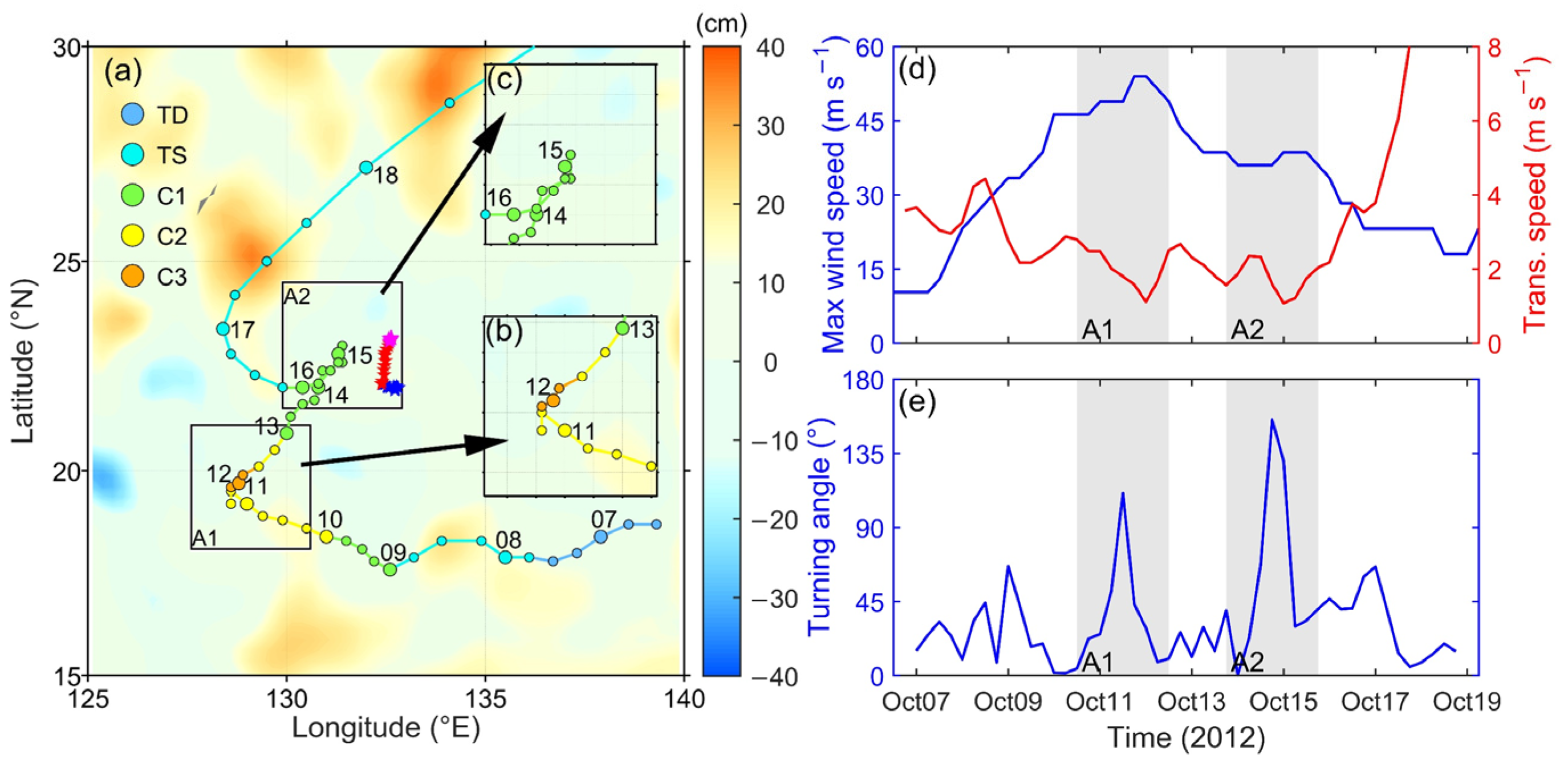
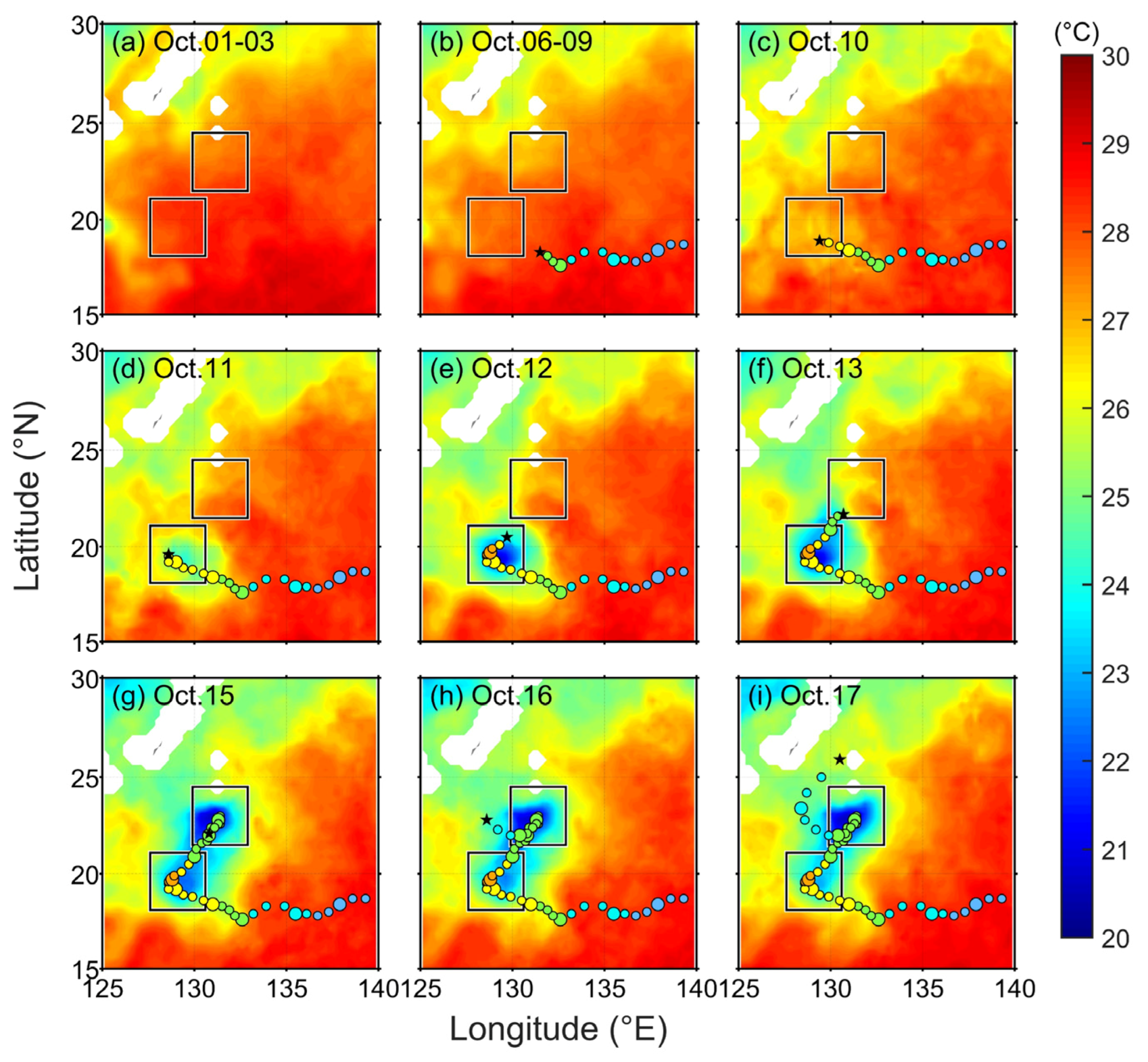
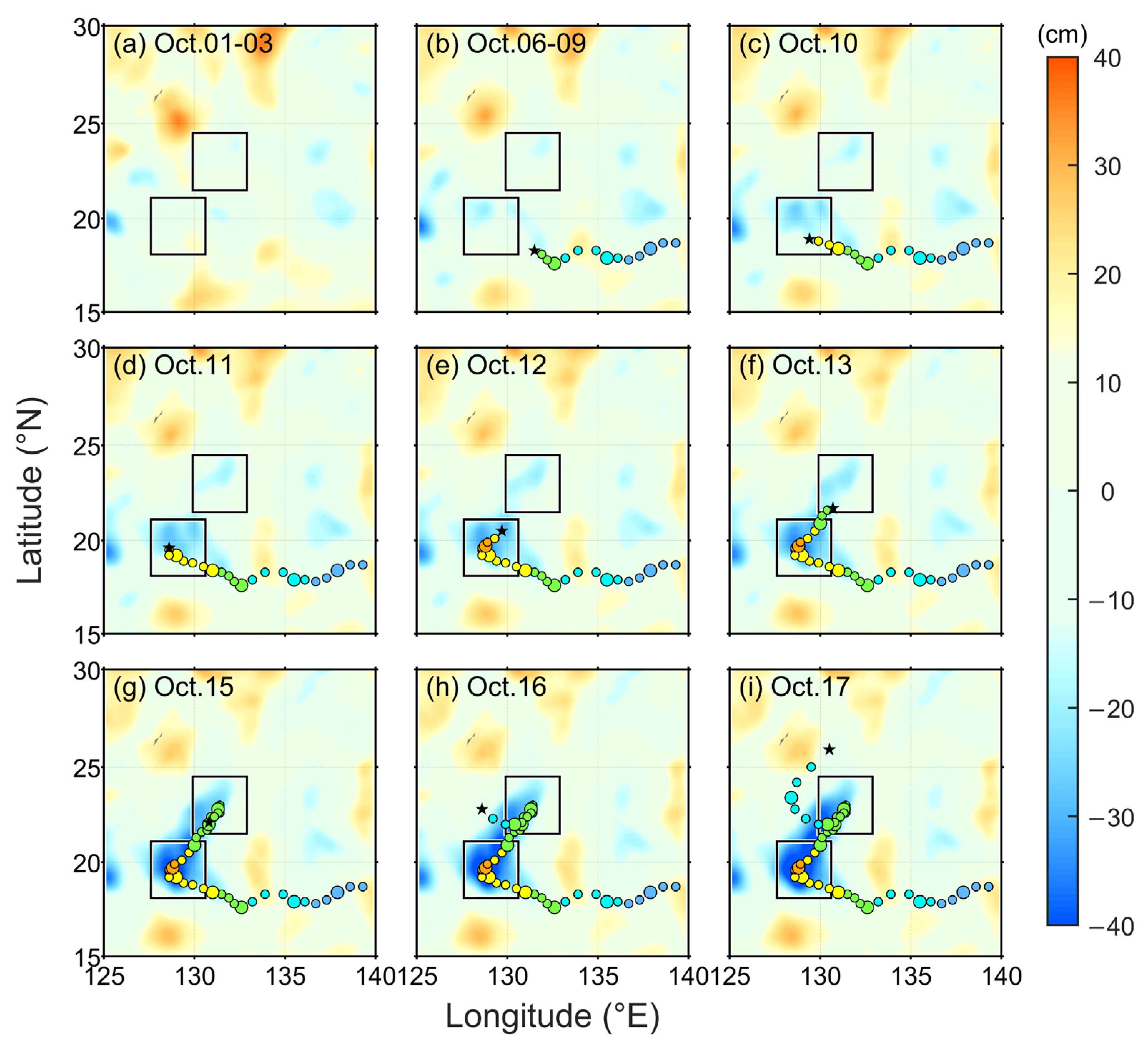
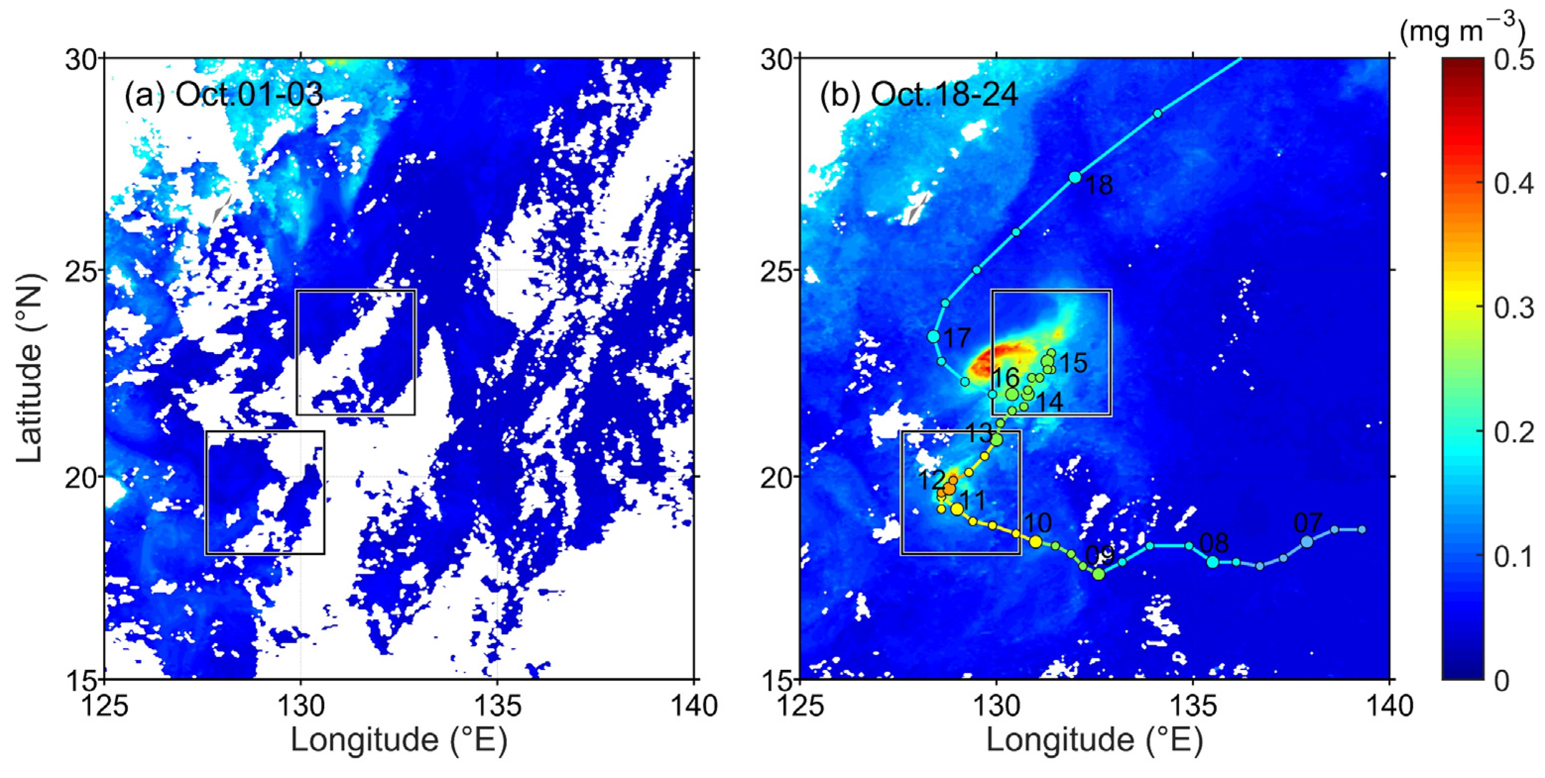
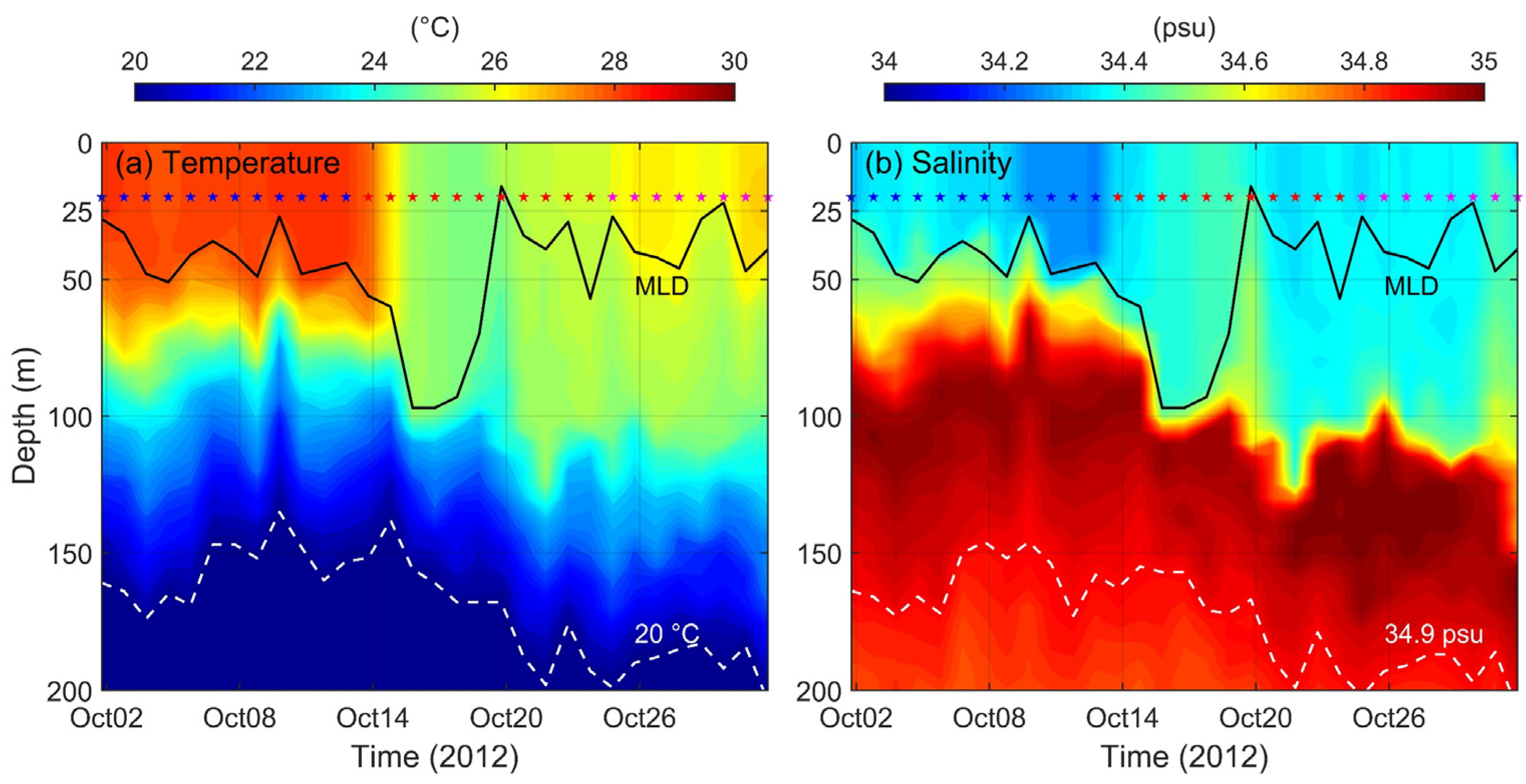
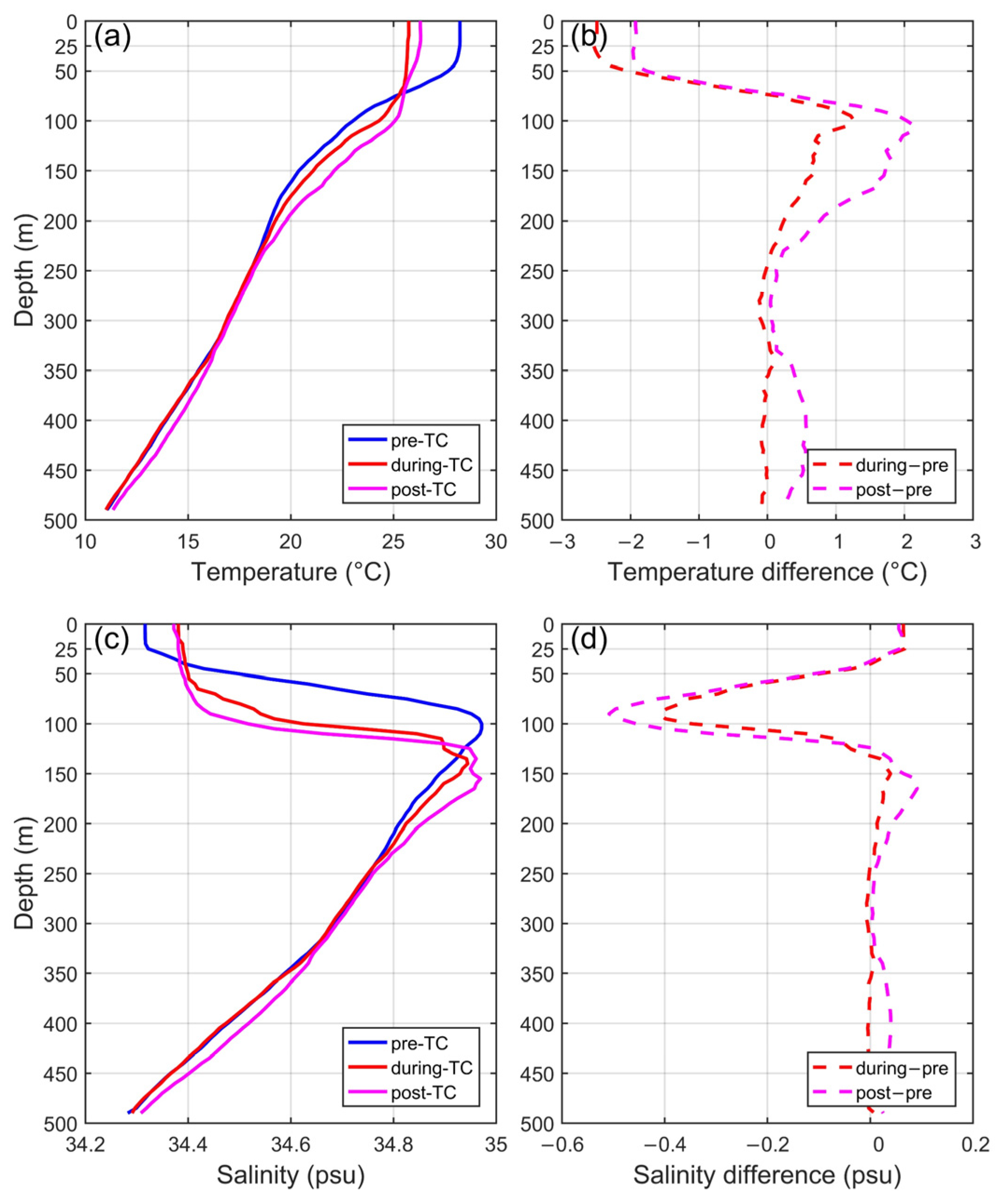
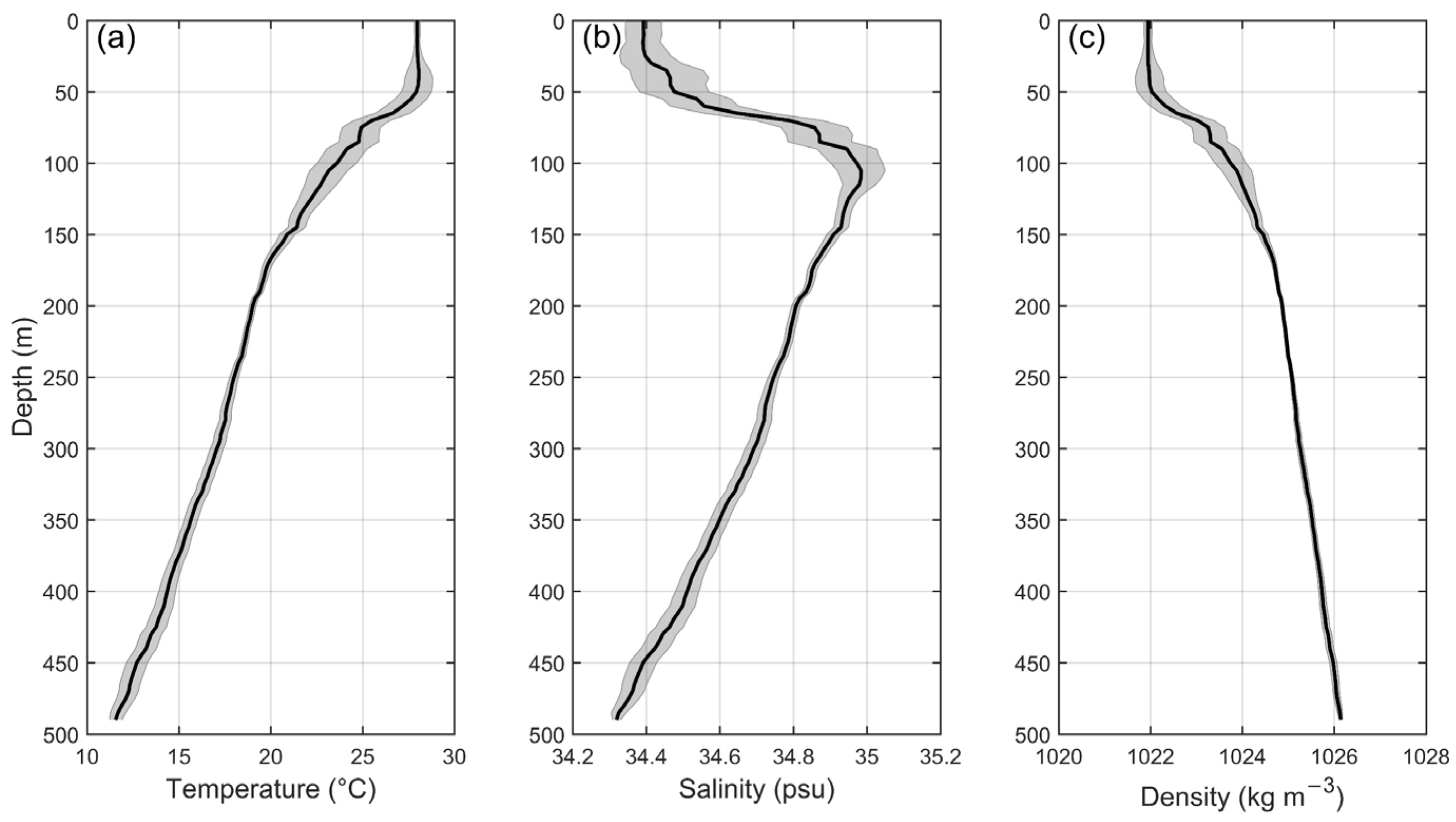
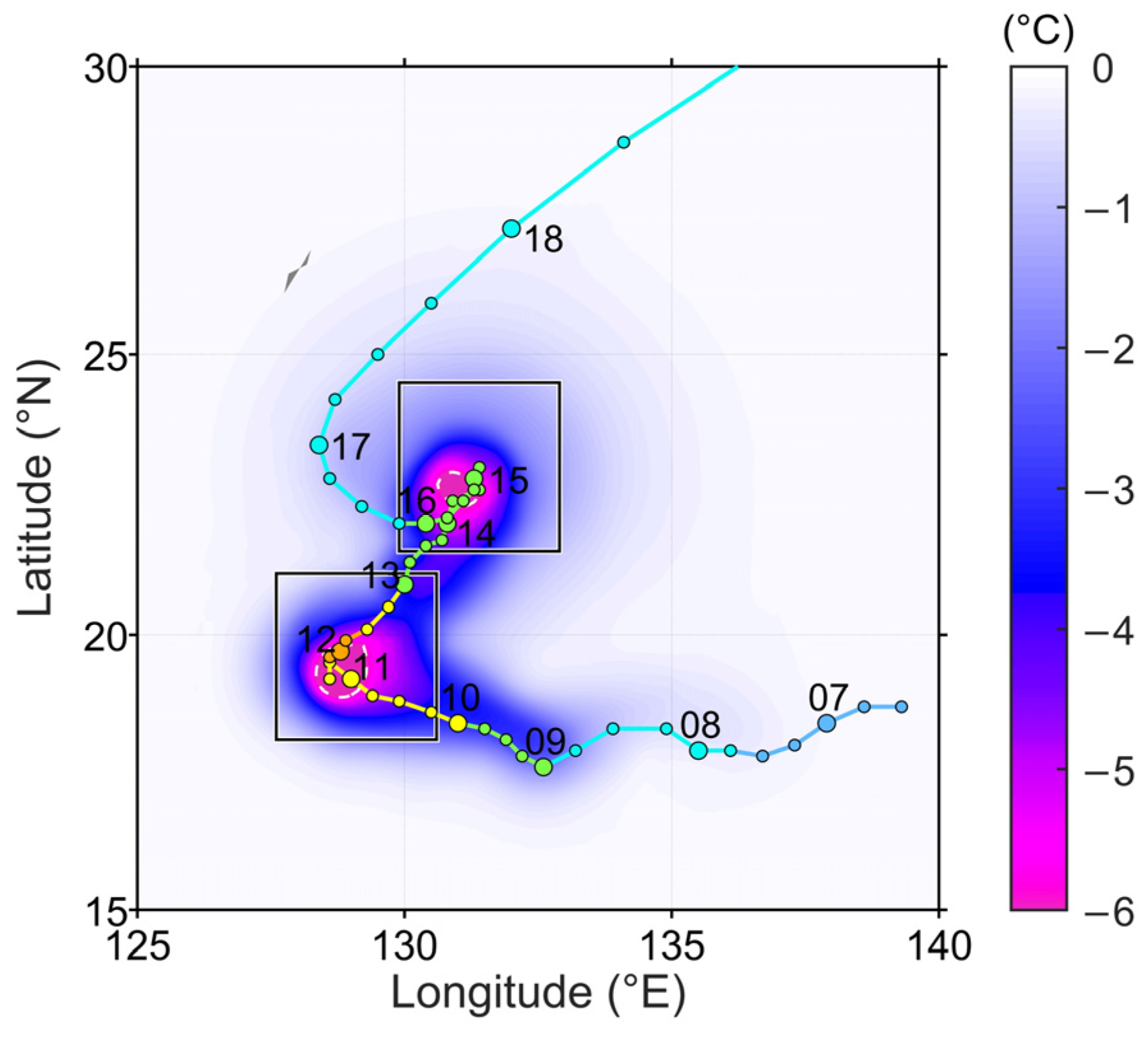
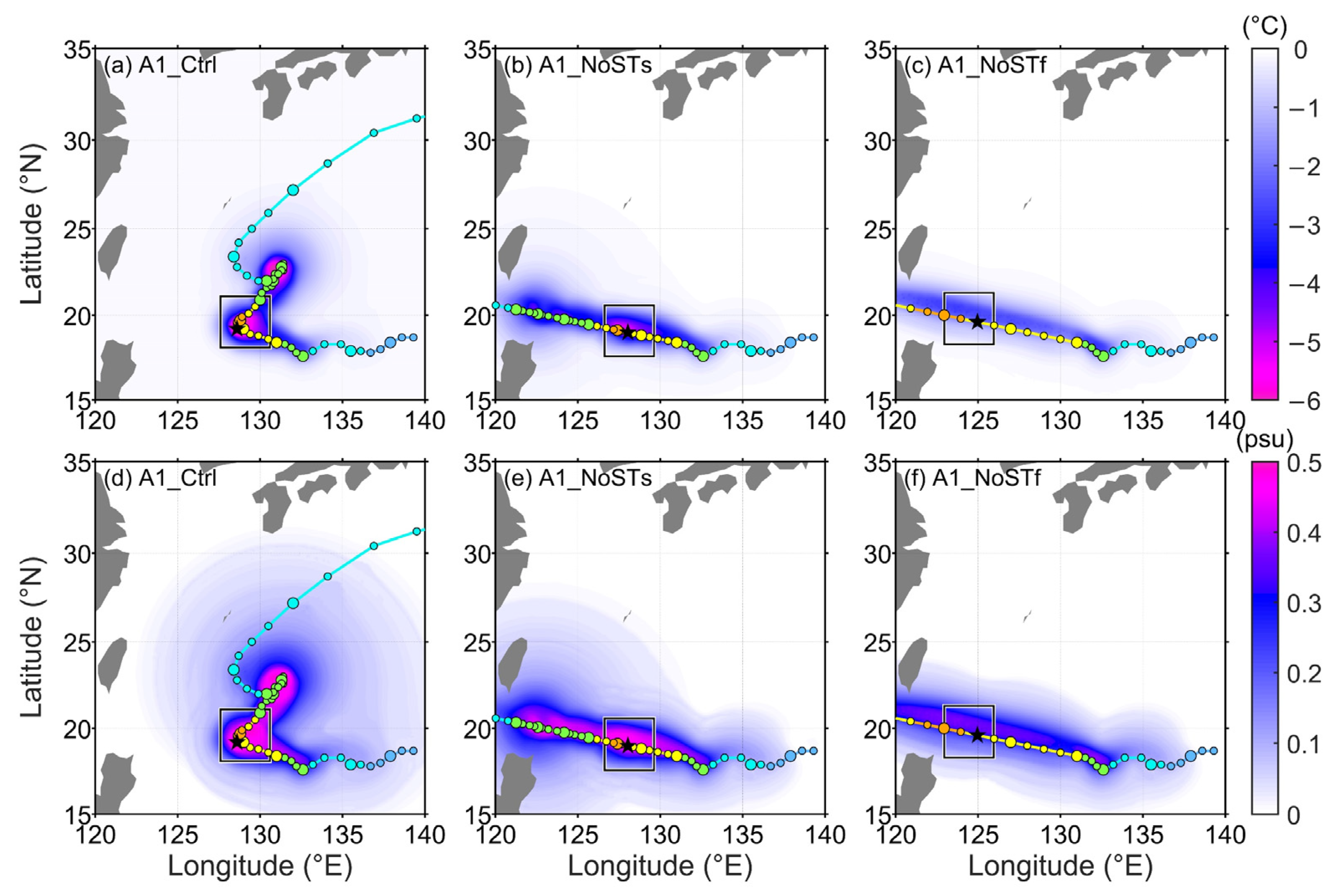
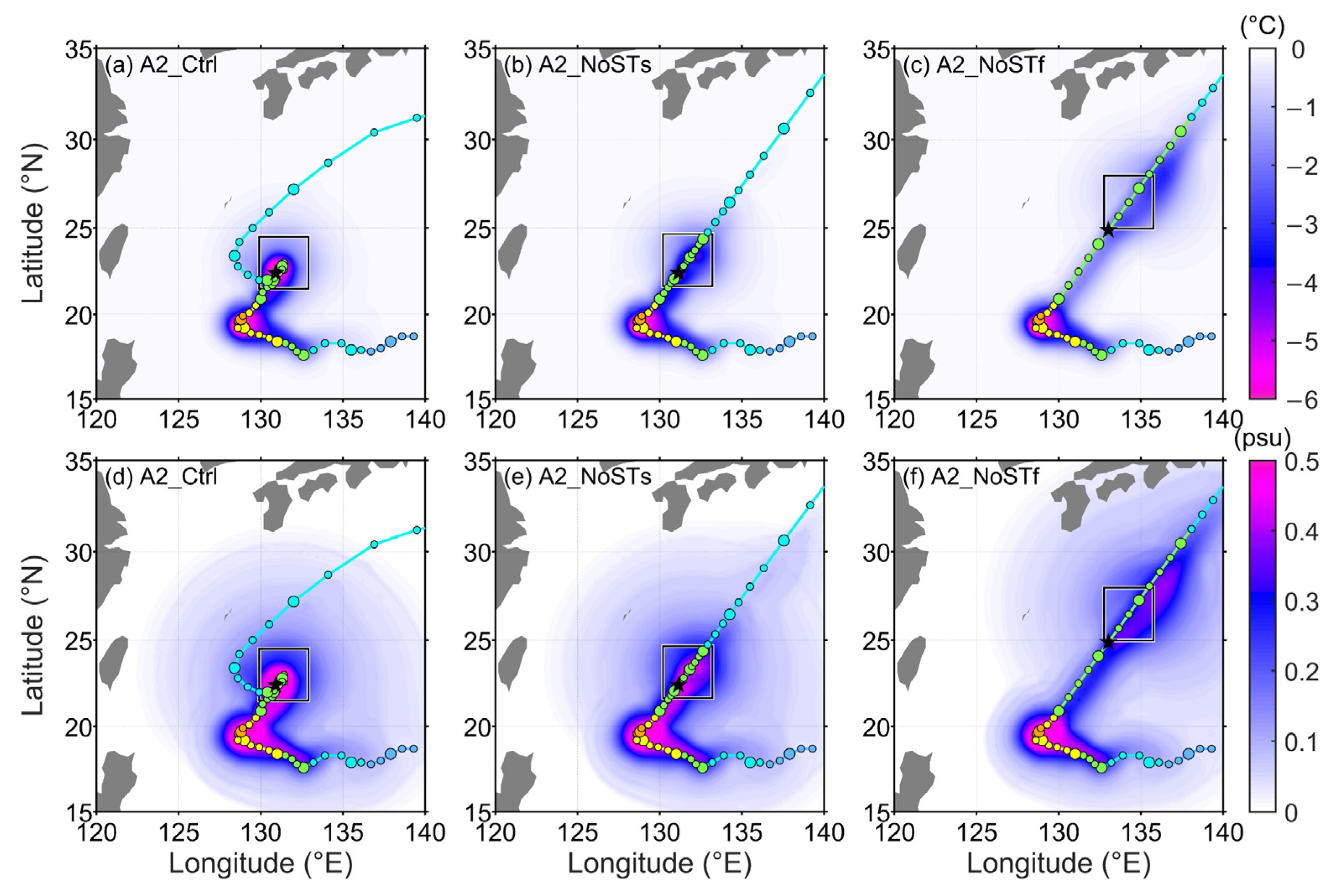
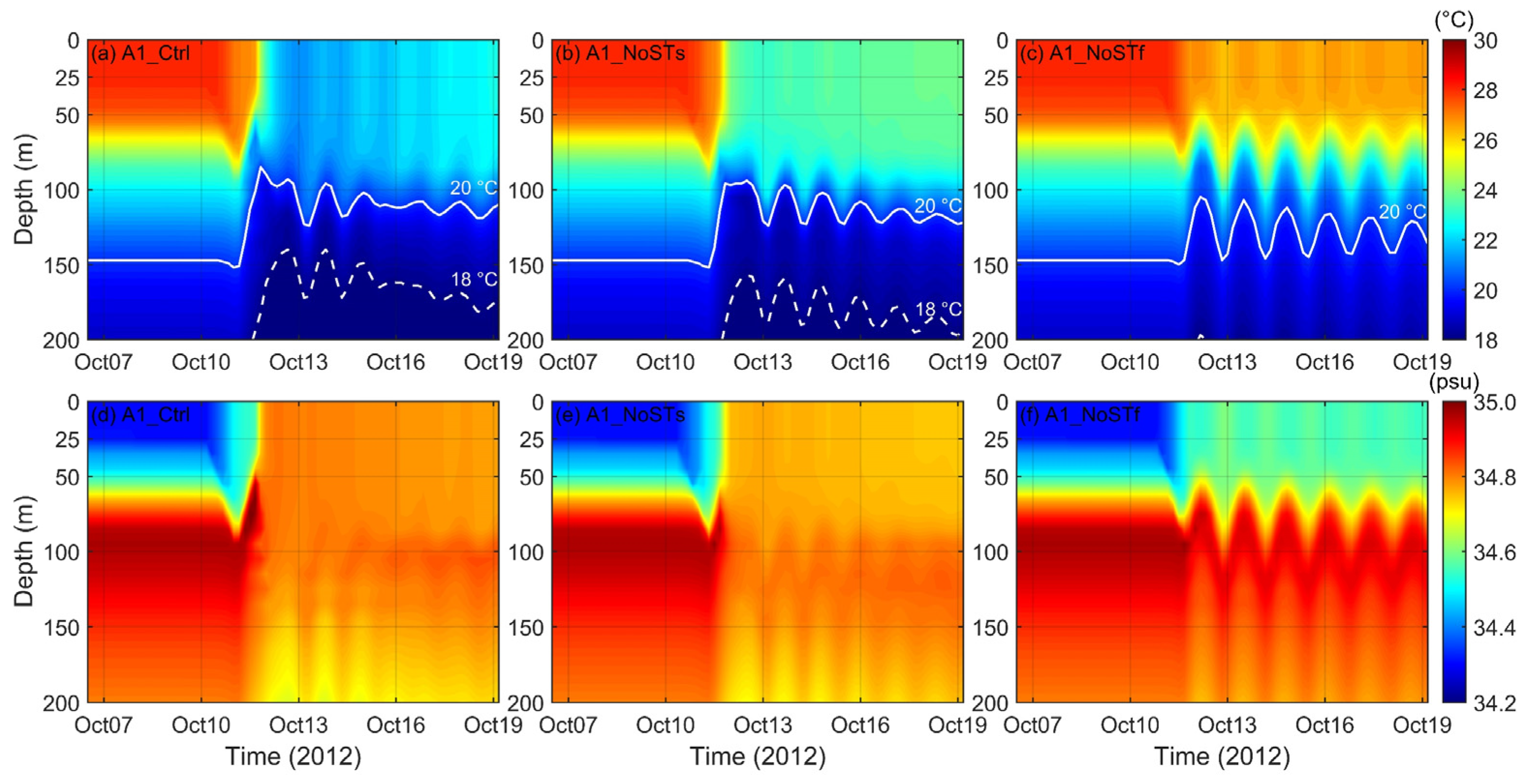
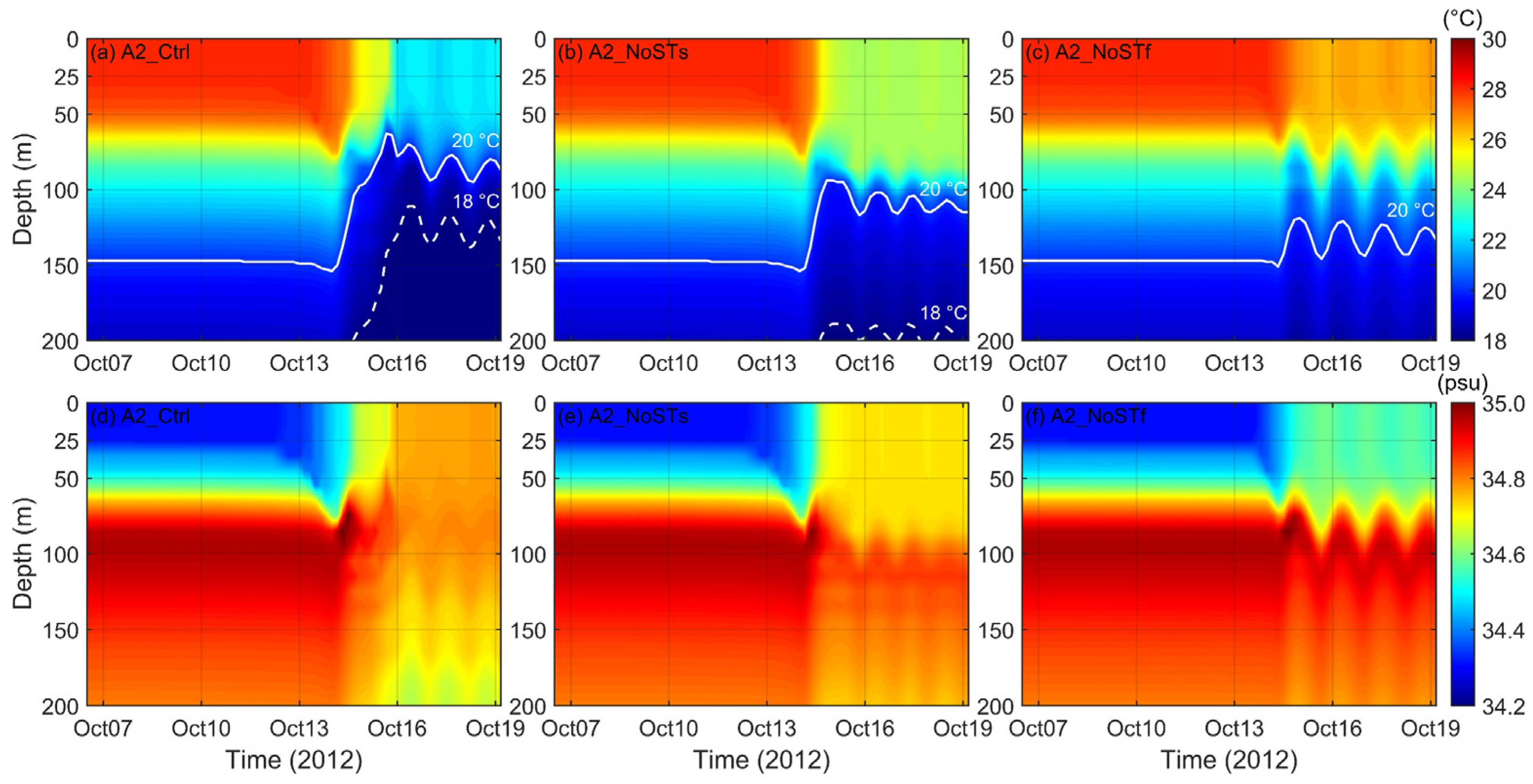
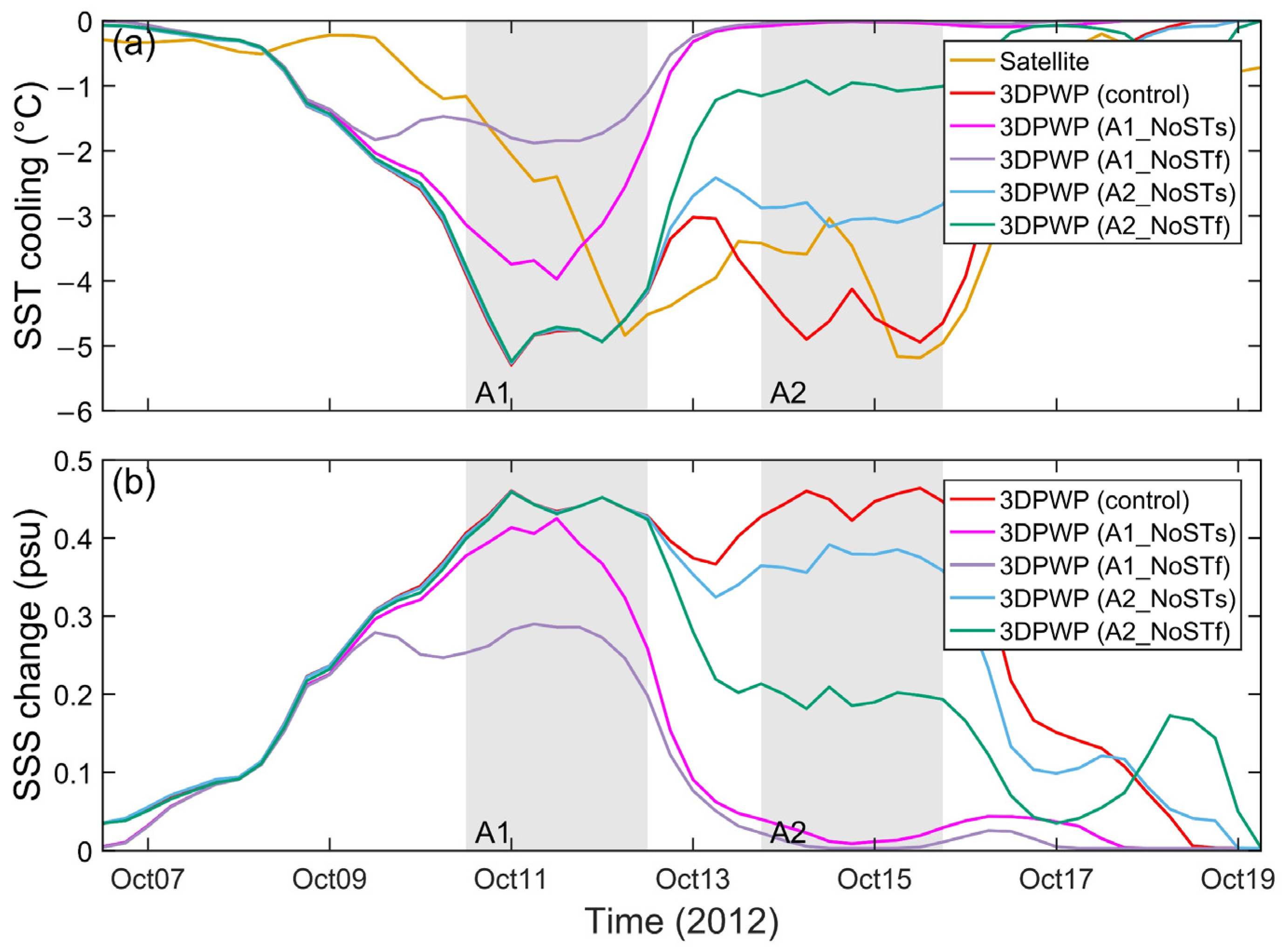
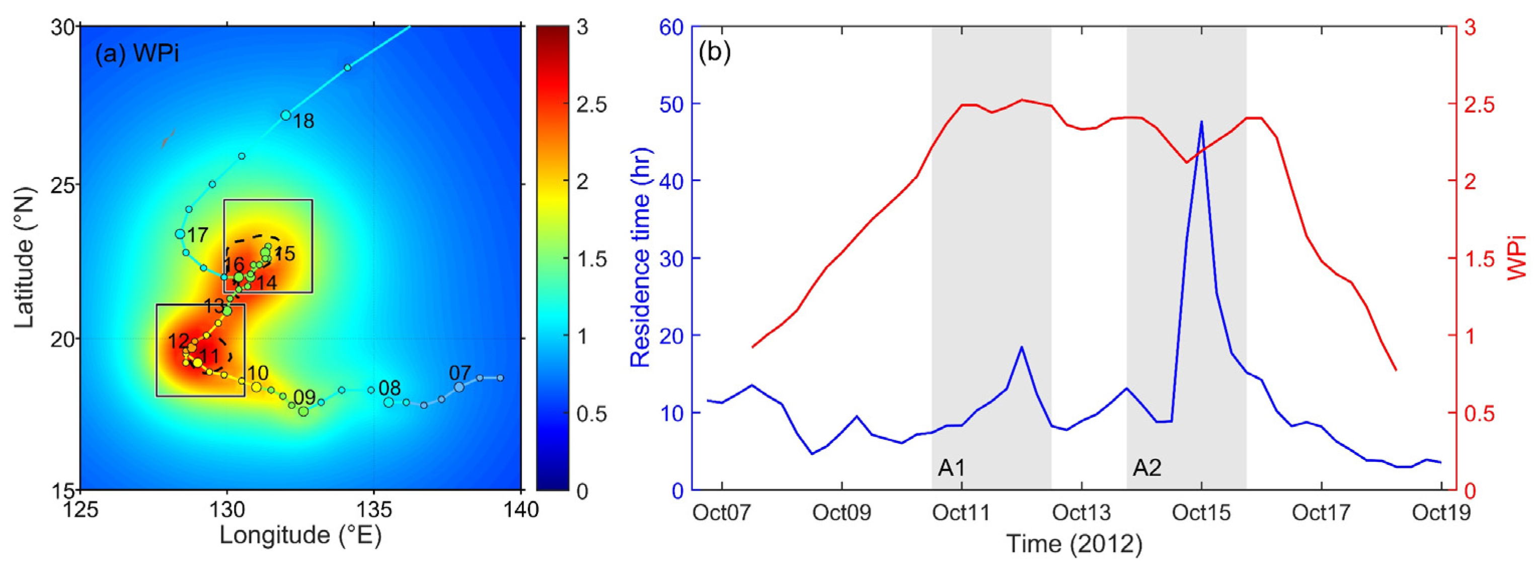
Table 1.
Model settings for the 3DPWP experiments.
| Experiments | Sudden Turning (ST) | Average Uh (m s−1) |
|---|---|---|
| A1_Ctrl | With ST | 2.0 |
| A1_NoSTs | No ST | 2.0 |
| A1_NoSTf | No ST | 5.0 |
| A2_Ctrl | With ST | 1.8 |
| A2_NoSTs | No ST | 1.8 |
| A2_NoSTf | No ST | 5.0 |
Table 2.
Maximum SST cooling, maximum SSS salinification averaged within 100 km of the typhoon centre, and contributions of sudden turning to SST cooling and SSS salinification in each 3DPWP experiment.
Table 2.
Maximum SST cooling, maximum SSS salinification averaged within 100 km of the typhoon centre, and contributions of sudden turning to SST cooling and SSS salinification in each 3DPWP experiment.
| Experiments | Maximum SST Cooling (°C) | Maximum SSS Salinification (psu) | Turning Contribution (%) |
|---|---|---|---|
| A1_Ctrl | 5.29 | 0.46 | 38.4 (SST) 23.5 (SSS) |
| A1_NoSTs | 3.98 (24.8% *) | 0.42 (8.7%) | |
| A1_NoSTf | 1.88 (64.5%) | 0.29 (37.0%) | |
| A2_Ctrl | 4.94 | 0.46 | 46.8 (SST) 28.0 (SSS) |
| A2_NoSTs | 3.17 (35.8%) | 0.39 (15.2%) | |
| A2_NoSTf | 1.16 (76.5%) | 0.21 (54.3%) |
* The percentage reduction compared with control Experiments A1_Ctrl and A2_Ctrl.
Disclaimer/Publisher’s Note: The statements, opinions and data contained in all publications are solely those of the individual author(s) and contributor(s) and not of MDPI and/or the editor(s). MDPI and/or the editor(s) disclaim responsibility for any injury to people or property resulting from any ideas, methods, instructions or products referred to in the content. |
© 2023 by the authors. Licensee MDPI, Basel, Switzerland. This article is an open access article distributed under the terms and conditions of the Creative Commons Attribution (CC BY) license (https://creativecommons.org/licenses/by/4.0/).
Share and Cite
MDPI and ACS Style
Zhang, Y.; Liu, Y.; Guan, S.; Wang, Q.; Zhao, W.; Tian, J. Sudden Track Turning of Typhoon Prapiroon (2012) Enhanced the Upper Ocean Response. Remote Sens. 2023, 15, 302. https://doi.org/10.3390/rs15020302
AMA Style
Zhang Y, Liu Y, Guan S, Wang Q, Zhao W, Tian J. Sudden Track Turning of Typhoon Prapiroon (2012) Enhanced the Upper Ocean Response. Remote Sensing. 2023; 15(2):302. https://doi.org/10.3390/rs15020302
Chicago/Turabian StyleZhang, Yihan, Yuhao Liu, Shoude Guan, Qian Wang, Wei Zhao, and Jiwei Tian. 2023. "Sudden Track Turning of Typhoon Prapiroon (2012) Enhanced the Upper Ocean Response" Remote Sensing 15, no. 2: 302. https://doi.org/10.3390/rs15020302
Note that from the first issue of 2016, this journal uses article numbers instead of page numbers. See further details here.