
Research and Evaluation on Dynamic Maintenance of an Elevation Datum Based on CORS Network Deformation

Chinese Academy of Surveying and Mapping, Beijing 100036, China
*
Author to whom correspondence should be addressed.
Remote Sens. 2023, 15(11), 2935; https://doi.org/10.3390/rs15112935
Submission received: 9 May 2023
/
Revised: 1 June 2023
/
Accepted: 2 June 2023
/
Published: 5 June 2023
(This article belongs to the Topic Development of Monitoring, Analysis and Maintenance Technics of Infrastructures)
Abstract
:This paper presents a method for dynamically maintaining a regional elevation datum using CORS stations as core nodes. By utilizing CORS station data and surface mass loading data (including land water storage, sea level, and atmospheric pressure), the normal height changes of each station can be determined and dynamically maintained. The validity of this method is verified using multiple leveling survey results from five CORS stations in Beijing’s subsidence area between January 2012 and June 2021. Results show that it is necessary to derive and correct the height anomaly variation of CORS stations caused by surface mass loading using the remove-calculate-restore method and the Green’s function integration method, with the influence of surface mass changes reaching a subcentimeter level. CORS stations exhibiting great observation quality achieve a mean accuracy of 2.7 mm in determining normal height changes. Such accuracy surpasses the requirements of second-class leveling surveys covering route lengths exceeding 1.35 km, as well as conforming/closed loop routes with distances greater than 0.46 km. By strategically selecting CORS stations with long-term continuous observations and high-quality data as core nodes within the elevation control network, dynamic maintenance of the regional elevation datum can be achieved based on CORS station data.
1. Introduction
Land subsidence in many regions of China caused by factors such as crustal movement, urbanization, groundwater extraction, and mineral resource development has led to inaccuracies in the regional height control networks [1,2,3], limiting the real-time accuracy and applicability of the height reference framework. Regular maintenance and updates of the framework are crucial to ensure its real-time relevance and applicability. In China, the elevation reference framework is implemented through two methods: the primary method used involves using leveling networks at various elevations to transfer height [4,5], while the other method employs GNSS and precise geoid models to measure the normal height of a point. With improvements in geoid model accuracy and resolution, the GNSS-based method has the potential to replace the method relying on leveling control networks [6,7,8]. However, for the maintenance and application of the height reference framework, a height control network based on leveling networks is currently indispensable.
The maintenance of a height control network through repeated leveling surveys is costly, time-consuming, and especially challenging in regions with frequent ground subsidence. China has established a national and multiple regional (provincial/municipal level) Continuously Operating Reference Station (CORS) networks for satellite navigation positioning [9,10]. These CORS networks can monitor the three-dimensional position changes of surface points with millimeter accuracy continuously and in all weather conditions [11]. If CORS stations are used as benchmarks to maintain a dynamic elevation reference framework, it could reduce leveling survey distances and frequency, lowering the costs and workload of maintaining the regional height reference frame. This approach has significant practical value for engineering purposes and warrants further research. Given that national-level elevation systems generally rely on the normal height system with respect to the geoid, whereas CORS station time-series observations are based on ellipsoidal heights referenced to the reference ellipsoid, a disparity in elevation anomalies arises between these two systems. As a result, this method also investigates the refinement of elevation anomalies to address this disparity and ensure consistency between the two systems [12,13,14].
This paper proposes a method for dynamically maintaining an elevation datum based on CORS station data. The CORS stations are used as the core benchmarks of the regional height control network, and the normal height changes of the stations are determined using continuous observation data and surface loading data. The normal height of each station is then dynamically corrected. The feasibility of this method is verified and analyzed using the CORS station network and leveling measurement data in a subsidence area of Beijing.
2. Method for Obtaining Normal Height Variations
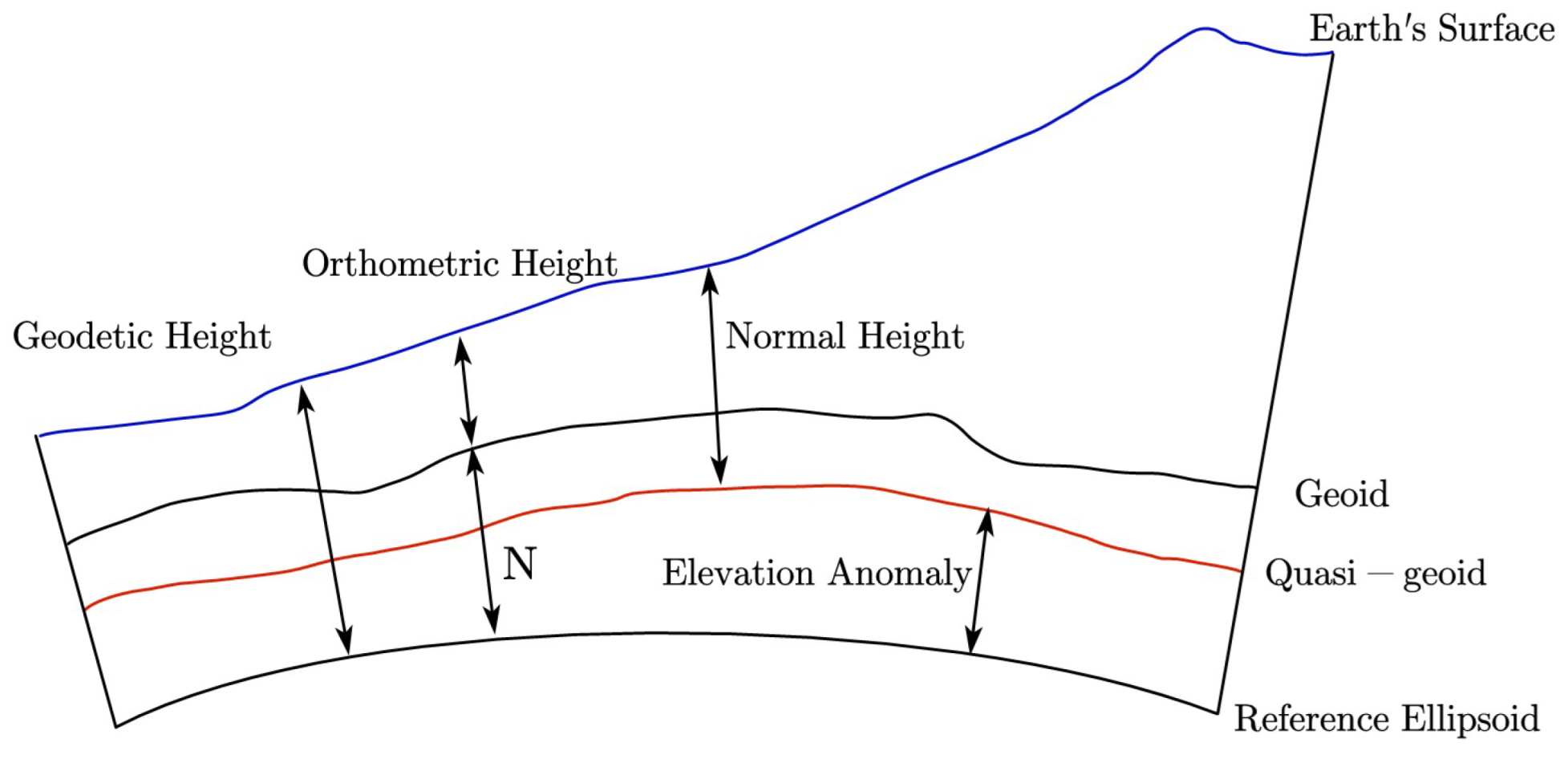
The geodetic height of a point on the earth’s surface consists of two components as shown in Figure 1 and Equation (1): is the orthometric height, is the elevation of the geoid, is the normal height, and is the elevation anomaly.
The elevation system adopted in China primarily employs the normal height system, with the quasi-geoid serving as the reference surface. Thus, to assess changes in normal height, one only needs to know variations in geodetic height and elevation anomaly. Variations in geodetic height can be obtained from CORS observation data, while variations in elevation anomaly can be calculated using surface loading models.
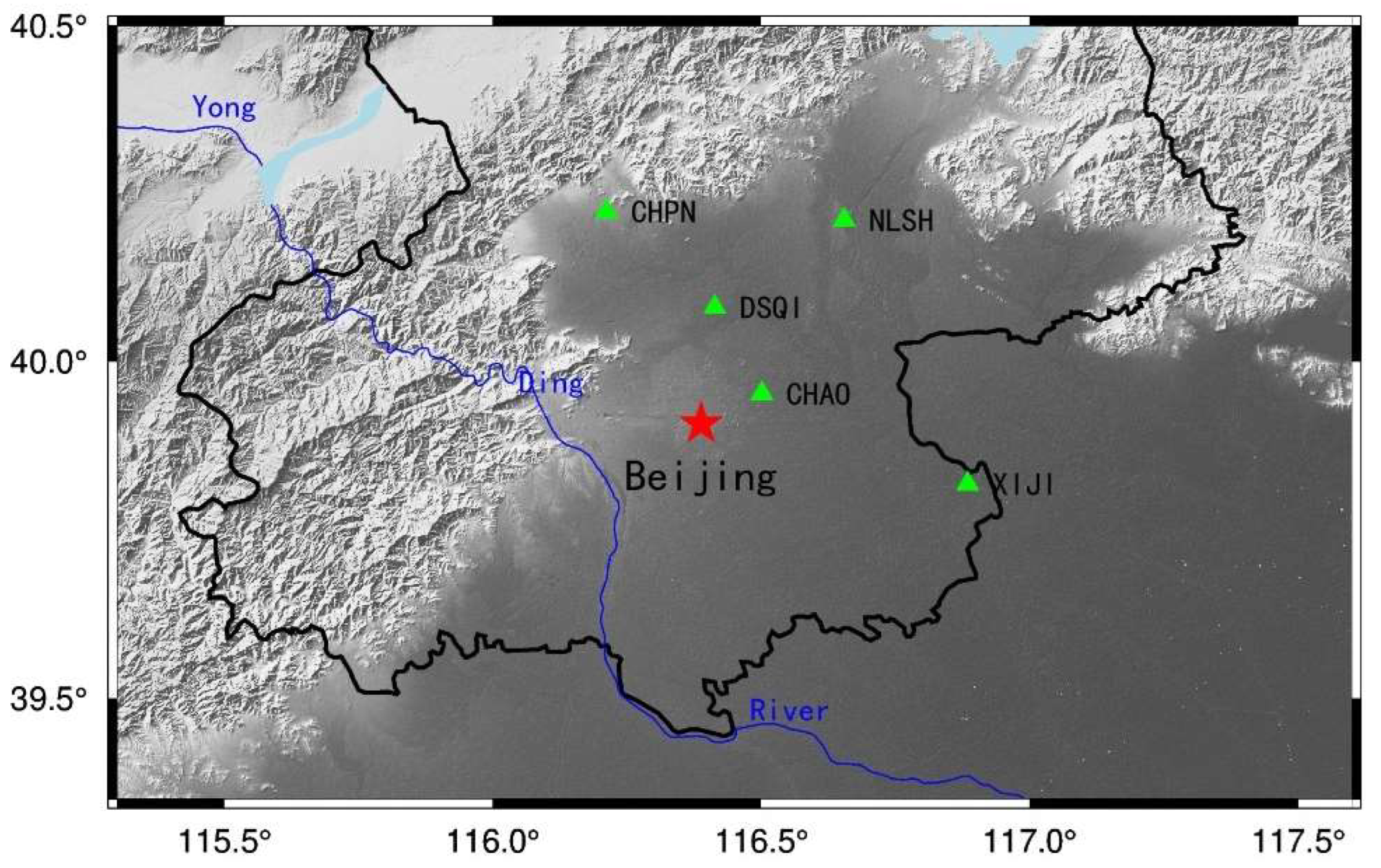
This paper uses the subsidence area of Beijing as a case study to demonstrate dynamic maintenance of the elevation reference system. The proposed technique involves five CORS stations—CHPN, NLSH, XIJI, CHAO, and DSQI—distributed as shown in Figure 2 for maintaining elevations in the subsidence area of Beijing.
3. Geodetic Height Variations Obtained from CORS Stations
Geodetic Height (GH) variations can be accessed from CORS station observations, which required pre-processing of the GNSS data using GAMIT/GLOBK software. The single-day regional loose solution of stations can be obtained by data solving the daily GNSS observation data for several parameters, including station location, receiver clock difference, and satellite clock difference. The constraints of coordinates, orbits, and other related parameters, however, in these single-day solution files, are generally loose. Therefore, it is necessary to unconstrain the single-day solution files of each CORS station for seven consecutive days after aggregation and then merge them into a comprehensive solution (weekly solution) based on the high-precision coordinates of the IGS station ITRF2014 frame using the Kalman filtering method.
Despite the processing, the observed time series still contains significant amounts of noise. This includes white noise (WH) with a constant power spectrum, flicker noise (FN) with a power spectrum inversely proportional to frequency, and random walk noise (RW) accumulated because of WH. Previous studies have revealed variations in noise characteristics across different regions [15]. For instance, a combination of WH and FN is more suitable for globally consistent models, while predominantly FN or RW models are better suited for the southern regions of California and Nevada. In China, a combination of WN, FN, and RW noise models is more appropriate.
To determine the GH variations, a weekly solution is also required to perform a time series analysis to obtain a fitted model characterizing the GH variations since the CORS signal is always accompanied by a lot of noise. In dealing with these noises, Wdowinski and Nikolaidis [16,17] proposed that the raw coordinate time series at reference stations exhibit high spatial correlation in height and that large-scale common deformation characteristics across a relatively wide area can obscure small-scale intranetwork deformation features. Therefore, they suggested the use of regional filtering methods to remove Common Mode Errors. Building on this approach, Dong [18] applied principal component analysis and Karhunen-Loeve transform for spatial filtering. Wavelet-based methods have demonstrated effectiveness in analyzing signal time–frequency localization, while the least squares variance component estimation method can provide accurate estimates of station motion parameters. Both methods have been applied to GNSS coordinate time series analysis. Amiri-Simkooei [19] used the least squares variance component estimation method to simultaneously estimate motion parameters for multiple IGS stations based on a combined model of white noise and scintillation noise. Wu [20] employed wavelet and wavelet packet denoising methods to eliminate both white noise and scintillation noise from GNSS coordinate time series. Li and Guo [21,22] combined wavelet and Fourier transforms to identify abrupt changes in geodetic measurement signals recorded in the time domain and extract the frequency range of signal discontinuities in the frequency domain.
Simulations were conducted in this paper using a noisy signal, where the underlying true signal was set to , and the random noise followed a normal distribution with a mean of 0 and a standard deviation of 0.0278. To perform denoising, we applied different wavelet functions with varying parameters to the simulated signal. The resultant denoised signals were evaluated, and the remaining noise levels were quantified. The denoising results, including the residual noise measurements, are summarized in Table 1. Clearly, different types of wavelets and parameter settings yield varying denoising results. This highlights that non-data-driven denoising methods, like the ones evaluated in this study, require a higher level of theoretical and technical expertise from personnel involved in the maintenance of elevation benchmarks.
The spatial filtering methods and wavelet analysis denoising discussed in the above studies both require significant human intervention. Spatial filtering methods necessitate the selection of an appropriate filter window length and filter function, while wavelet analysis requires selecting an appropriate wavelet to mitigate overprocessing and incomplete processing issues. Given these challenges and limitations imposed by the uncertainty principle, this paper has opted for a data-driven, nonlinear, and non-stationary signal processing method—the Complete Ensemble Empirical Mode Decomposition with Adaptive Noise (CEEMDAN) method. By leveraging data-driven techniques, this method automatically extracts the local features of signals based on the characteristics of actual signals and processing requirements [23,24]. CEEMDAN is an improved version of Empirical Mode Decomposition (EMD), first proposed by E. Huang [25,26]. The EMD method posits that any signal can be decomposed into the sum of several Intrinsic Mode Functions (IMFs) satisfying two constraints:
- i.
- The number of extreme points and the number of zero crossing points differ by no more than one across the entire data segment.
- ii.
- At any moment, the average value of the upper envelope formed by the local extreme value points and the lower envelope formed by the local minimal value points is zero.
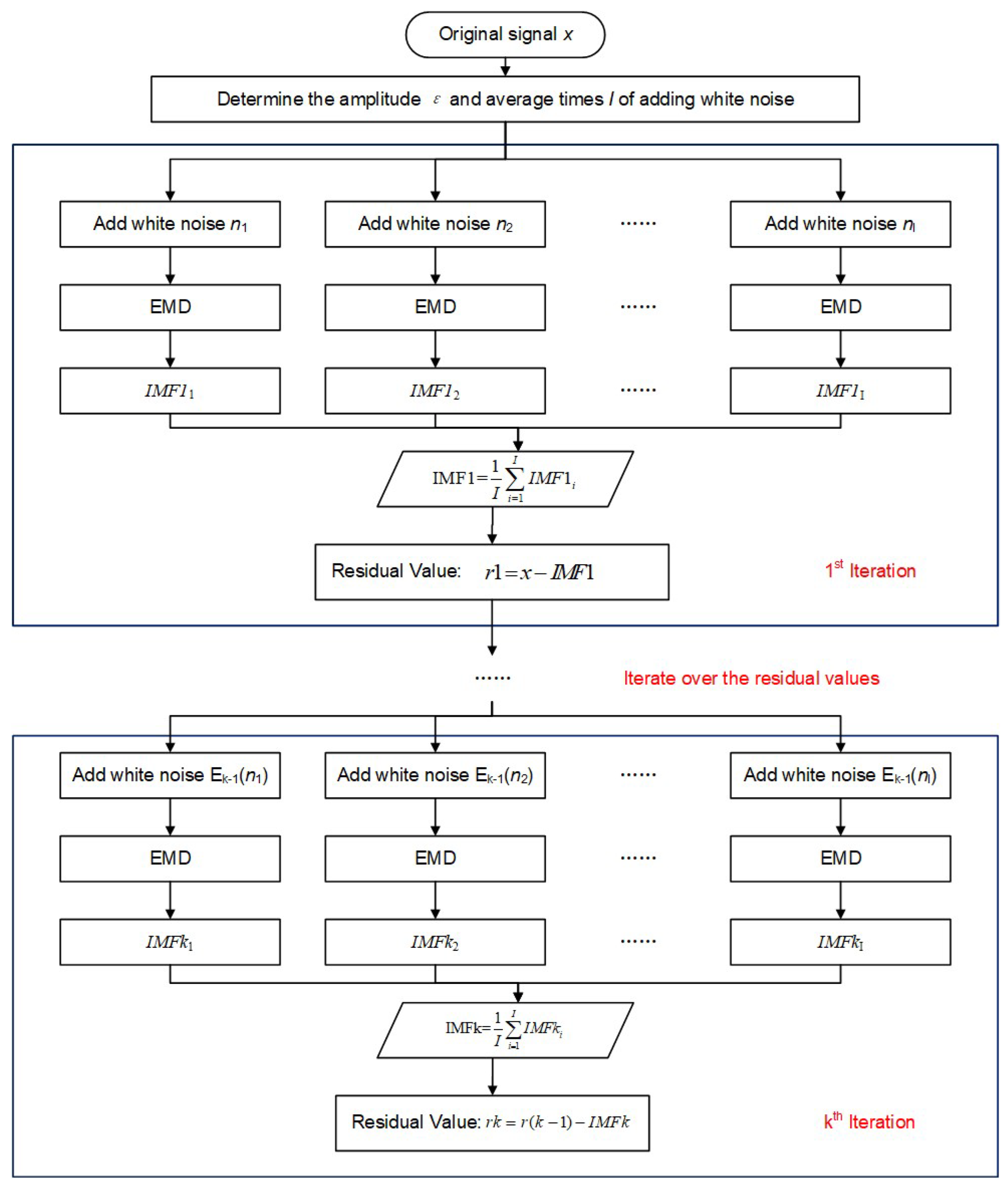
The individual components of the IMF represent each frequency component of the original signal and are arranged in order from high to low frequency. However, the IMF obtained by EMD suffers from modal aliasing, where signals of different feature scales can be present in one IMF component or signals of the same feature scale can be dispersed into different IMF components. CEEMDAN improves upon EMD by exploiting the property that white noise has a mean value of 0. It achieves better decomposition results by introducing uniformly distributed white noise or IMF components of white noise several times during each decomposition process. Figure 3 illustrates the flowchart of the CEEMDAN algorithm, where denotes the order IMF of .The result from the CEEMDAN is as Formula (2):
The high-frequency IMF can be considered as noise and rejected. The low-frequency IMF represents the trend component of CORS station data, while the remaining IMFs capture the periodic variations of the station. These periodic and trend terms must be fitted separately to obtain the GH variation time series.
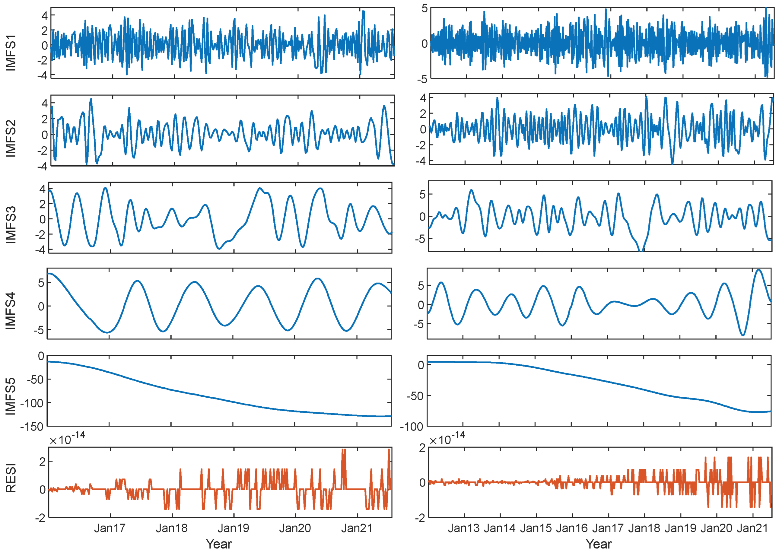
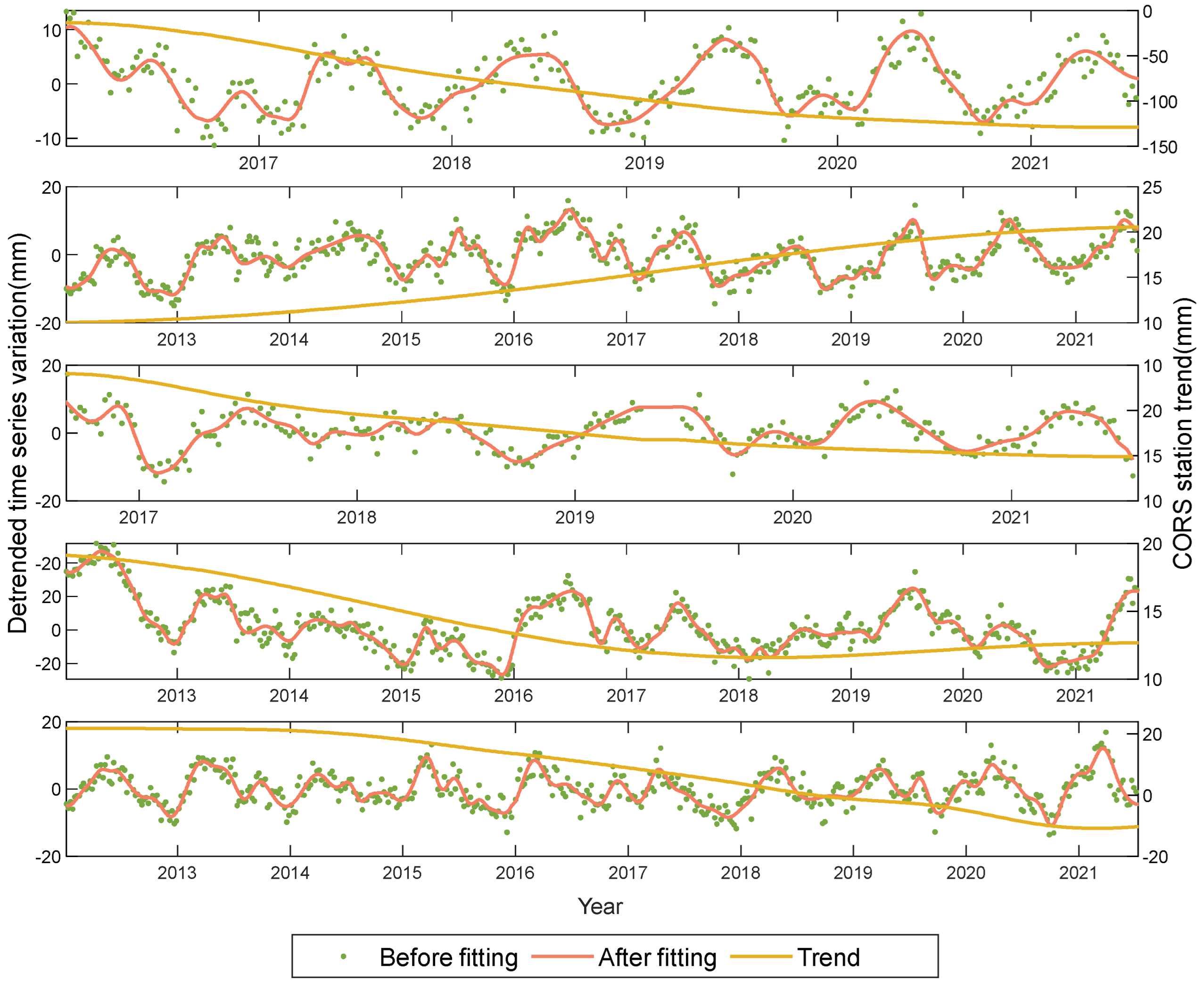
Figure 4 illustrates the outcomes of applying CEEMDAN to data from the CHAO and XIJI CORS stations. The method effectively decomposes the high-frequency noise, medium-frequency periodic signal, and low-frequency trend signal present in the observation data. Specifically, IMF1 and IMF2 correspond to high-frequency noise signals, IMF3 represents a mixture of some periodic signals at medium frequencies, IMF4 corresponds to the annual signal, and IMF5 captures the motion trend of the CORS stations. After ignoring noisy signals at high frequencies, the periodic and trend signals are interpolated and smoothed with linear interpolation and smooth spline fitting, respectively. The result is a GH variation time series with a one-day time resolution. Figure 5 presents the time series results for the five CORS stations—CHAO, CHPN, XIJI, NLSH, and DSQI.
Two accuracy indicators, Root Mean Square Error (RMSE) and Goodness of Fit (GF), are used to quantitatively assess the results of CORS station GH variation time series fitting. RMSE, calculated using Equation (3), measures the degree of deviation between the fitted and observed values, with smaller values indicating less deviation. GF, calculated using Equation (4), indicates the goodness of fit, with values closer to 1 implying a better fit. The Signal-to-Noise Ratio (SNR) is utilized to evaluate the observation quality of CORS stations, and its computation formula is presented in Equation (5). Higher SNR indicates better observation quality. Assessment of observation quality and fitted signal for CORS stations is shown in Table 2.
indicates the period signal of the fitted estimate, indicates the trend signal of the fitted estimate, indicates the observed GH variations, and is the number of samples.
denotes signal power, denotes noise power, and lower indicates higher noise content.
The accuracy assessment reveals that the RMSE of all five CORS stations is below 3 mm, indicating a very low deviation in the fitting results. CHAO, DSQI, and NLSH all achieved GF values above 0.97. However, due to high noise influence caused by low SNR, CHPN and XIJI both had lower GF values.
4. Elevation Anomaly Variations Caused by Surface Loading
The geoid is not static and changes due to the Earth’s surface and internal mass migration. This change is mainly attributed to various global dynamic processes, including land water storage changes (including groundwater), fluctuations in sea and glacial levels, glacial isostatic adjustment (GIA), tectonic uplift and subsidence, and earthquakes [12,13,14]. In most regions of China, variations in land water storage (including groundwater), sea level, and atmospheric pressure are the primary contributors to changes in the geoid.
The remove-compute-restore method, which is used to determine the static geoid, can be applied to divide changes in the geoid at a point on the Earth’s surface into far-field and near-field contributions. The global uniformly distributed mass element change undergoes spherical harmonic expansion to obtain loading spherical harmonic coefficients that are combined with loading Love numbers to perform a spherical harmonic synthesis calculation. This determines the contribution of global mass element change to the geoid change at the point in question, which represents the reference of the geoid change at the point and is defined as the far-field contribution [27,28]. By integrating surface mass element changes within a certain range of the Earth’s surface point in question, together with the global mass element spherical harmonic expansion model, and by using the remove-compute-restore method and mass loading Green’s function integration [29,30,31], more detailed spectral information on height anomaly change can be obtained. The effect of surface mass element changes within this range is referred to as the near-field contribution. Since geoid changes are generally at the millimeter level, this discussion assumes that height anomaly variations are equivalent to geoid changes.
Figure 6 illustrates the main process for calculating high-precision regional height anomalies using the remove-compute-restore method. Firstly, the global surface mass model that reflects the intermediate-to-long wavelength signals in the region of interest undergoes spherical harmonic analysis to calculate the reference height anomaly variations and equivalent water height in the reference area. Then, the regional high-precision surface mass model that reflects the short wavelength signals in the region of interest is subtracted by the equivalent water height in the reference area. The residual equivalent water height is integrated using Green’s function to obtain the residual height anomaly variations. Finally, the reference and residual height anomaly variations are combined and restored as the regional height anomaly variations.
4.1. Calculation of Far-Zone Contribution
The Earth’s surface atmosphere [29], land water storage, and sea level [32] changes are non-tidal, and these surface non-tidal loading changes can be expressed uniformly by the equivalent water height changes at the ground surface. The equivalent water height at the ground point can be expressed as the normalized loading spherical harmonics, which is calculated in Equation (6).
where: denote the ground point distance from the center of the earth, and the ground point co-latitude and longitude, respectively; and denote the th degree th order normalized loading spherical harmonic coefficients; and is the fully normalized Legendre function.
From the theory of surface mass loading deformation, it is known that the reference height anomaly caused by the change in surface mass loading is determined by Formula (7).
where is the universal gravitational constant, is the total mass of the Earth, is the density of water, is the average density of the Earth’s crust, is the radius of the long semi-axis of the Earth, is the normal gravity, and is the th degree loading Love-number.
The land water global data used in the study of reference height anomaly at CORS is the Global Land Data Assimilation System (GLDAS) data from NASA and the National Centers for Environmental Prediction. The data are derived from land surface modeling and data assimilation techniques [33,34] to output land surface hydrological parameters at a spatial resolution of 0.25° × 0.25° monthly. The global data used for atmospheric pressure are the European Centre for Medium-Range Weather Forecasts (ECMWF) global atmospheric pressure model at a spatial resolution of 0.25° × 0.25° monthly [35]. The global data used for sea level are the Maps of Sea Level Anomaly (MSLA) provided by the Archiving, Validation, and Interpretation of Satellites Oceanographic Data (AVISO) of the Centre National d’Etudes Spatiales (CNES), which is generated from the monthly mean sea surface height anomalies from multiple global satellite altimetry at a spatial resolution of 0.25° × 0.25° monthly (Resource of the data can be found in the supplementary material part).
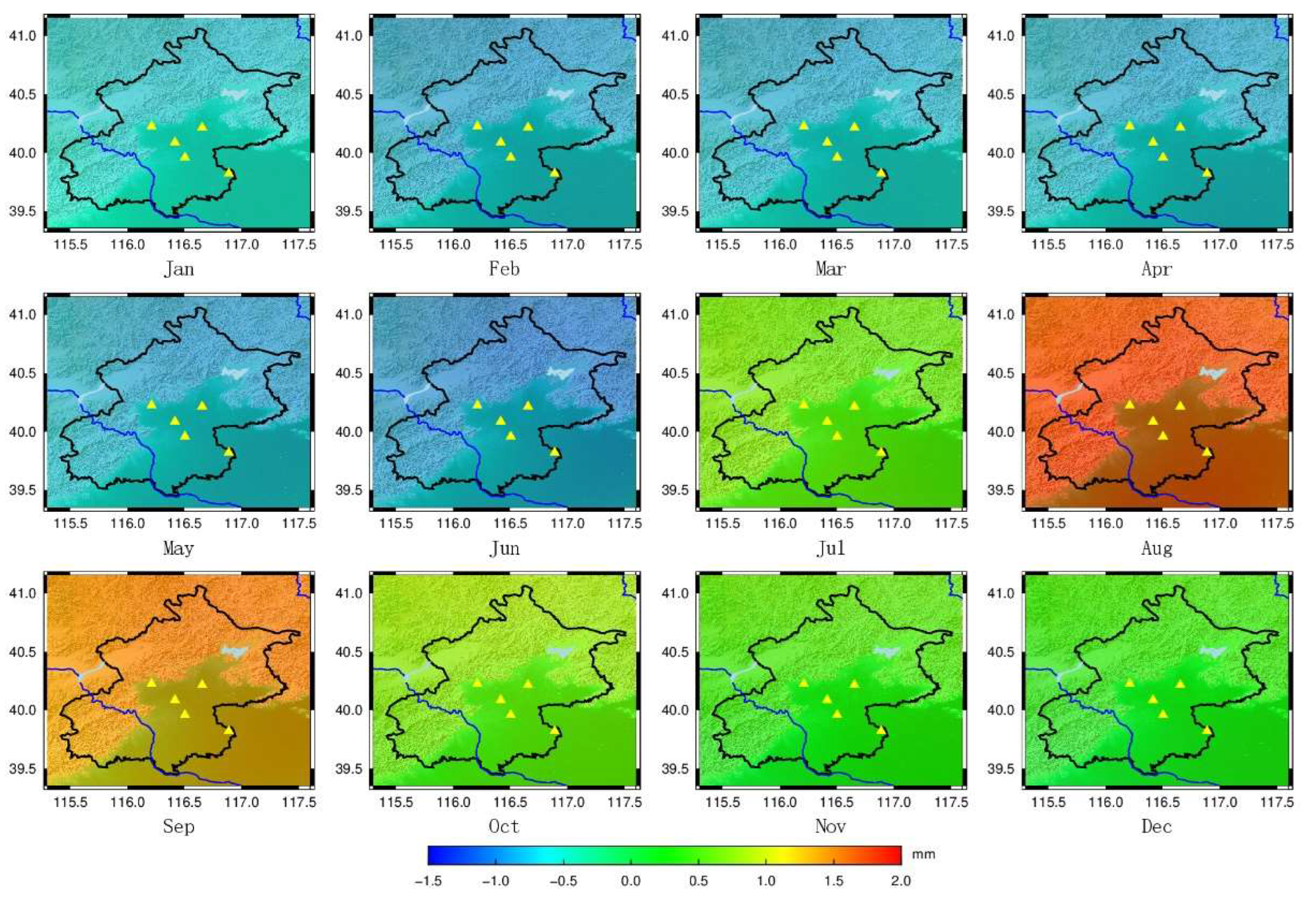
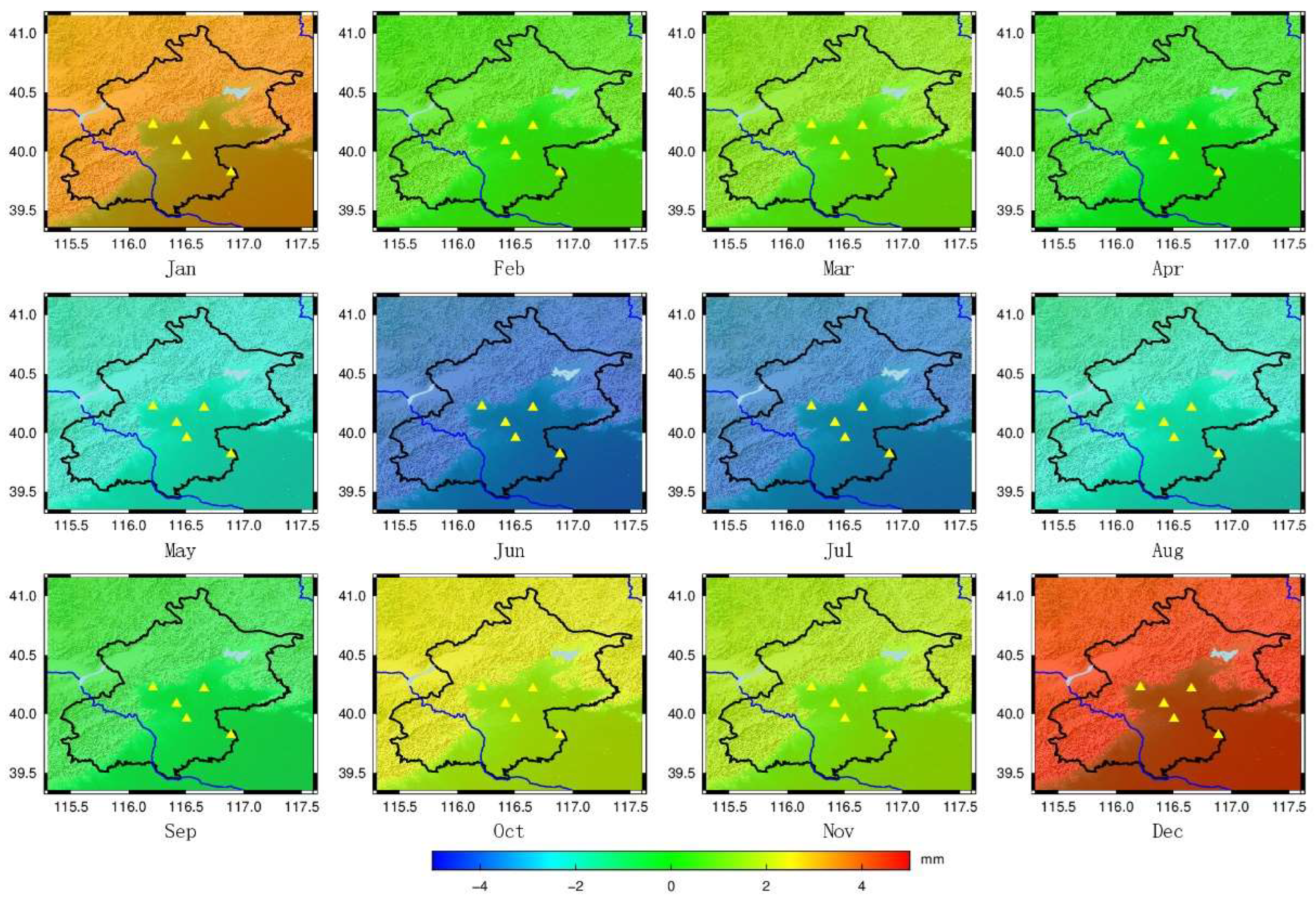
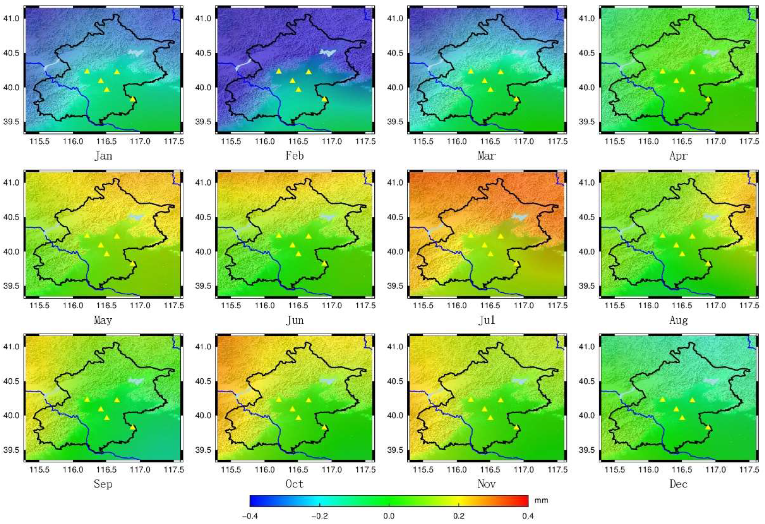
The reference height anomaly variations caused by global terrestrial water changes, global atmospheric pressure changes, and global sea level changes in the subsidence area of Beijing can be calculated using the global loading data. Some of the calculated reference height anomaly variations are shown in Figure 7, Figure 8 and Figure 9.
4.2. Calculation of Near-Zone Contribution
The gravitational potential directly generated by the surface mass near the ground point is (8).
The unit mass produces a loading on the solid Earth, and the Earth is thus deformed, which in turn indirectly causes gravitational potential (9).
where is the value of gravity, p is the fully normalized associative Legendre function, is the spherical angular distance between the calculated point and the ground flow point , and the cosine of is calculated as Equation (10):
The gravitational potential due to unit mass is the sum of the direct and indirect gravitational potential, and (11) can be obtained according to Equations (8) and (9)
Provided that the equivalent water height change due to surface mass loading is , the geoid change is the spatial convolution of with the Green’s function (12).
where is the flow integration surface element, and the integration radius is generally taken as 200~300 km.
The regional data used for calculating residual height anomaly variations in this paper are from the Chinese Land Data Assimilation System (CLDAS)-V2.0 data, containing barometric pressure data and soil water data, at a spatial resolution of 0.0625° × 0.0625° daily(Resource of the data can be found in the supplementary material part).
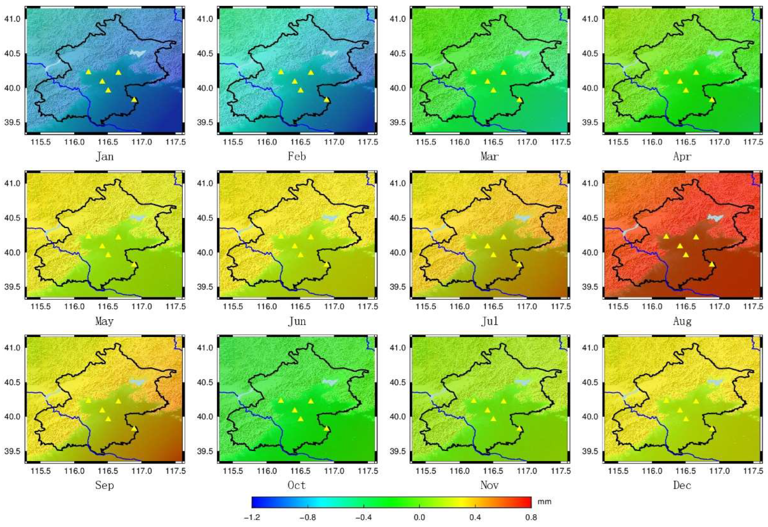
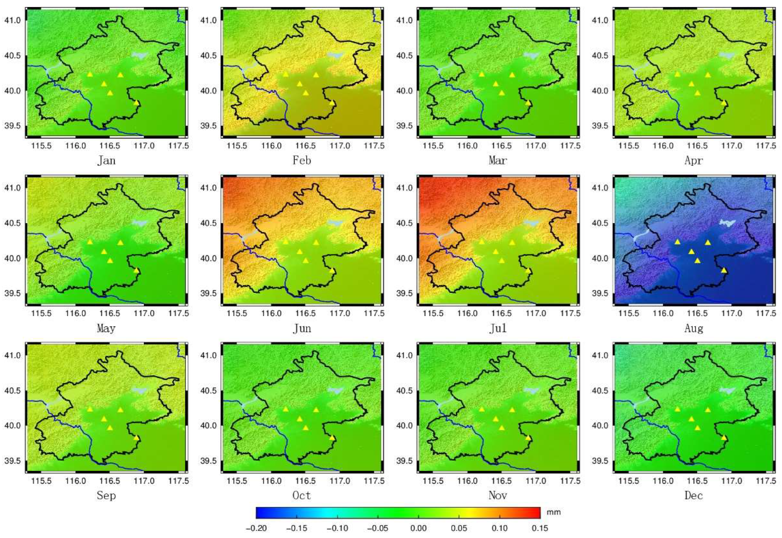
The residual height anomaly variations caused by regional terrestrial water changes and global atmospheric pressure changes in the subsidence area of Beijing can be calculated using the aforementioned regional loading data. Some of the calculated residual height anomaly variations are shown in Figure 10 and Figure 11.
4.3. Restoration of Regional Height Anomaly Variation
After clarifying the far-zone and near-zone contributions to the height anomaly change, a more refined variation can be derived by using the remove-compute-restore method. The restored results of some of the regional height anomaly variations are shown in the Figure 12.
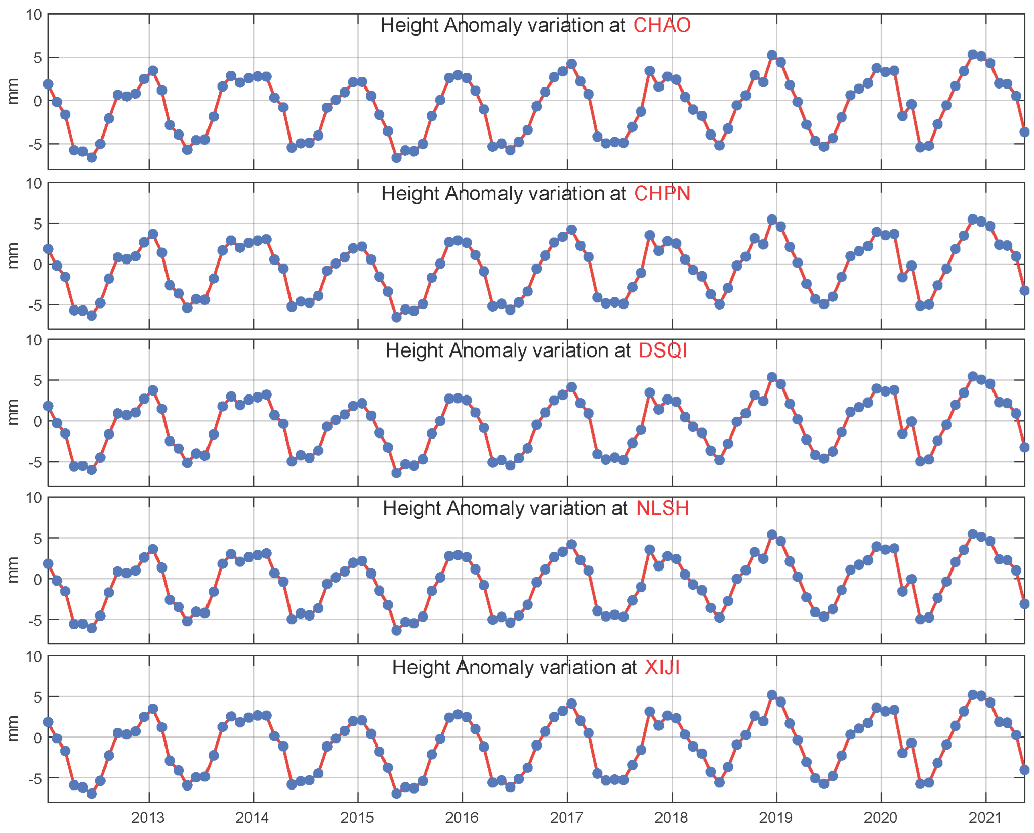
This is also a calculation method for the regional loading deformation field. By calculating the loading deformation field of the Beijing area every day from 2012 to 2021, it is possible to obtain temporal results of height anomaly variation in five CORS stations, as shown in Figure 13 The statistical table of height anomaly changes in these five CORS stations can be found in Table 3.
Based on Table 3 and Figure 12, it can be seen that the height anomaly variation caused by surface loading exhibits clear periodic changes with variations from year to year, and the change varies between −6 mm and 5 mm. To achieve high-accuracy normal height solutions for CORS stations, it is necessary to introduce corrections for the height anomaly changes.
5. Calculation and Validation for Normal Height Variations
By referring to the schematic diagram in Figure 1, the Normal Height (NH) variation of CORS stations can be calculated using Equation (13).
where is the NH variation, represents the geodetic height variation obtained from CORS stations, and is the height anomaly variation obtained from surface loading. The RMSE is calculated using Equation (14).
where and represent the geodetic height RMSE at times and , respectively, and represents the corresponding height anomaly variation. The height anomaly is estimated based on a 20% uncertainty.
To validate the NH variation calculation method proposed in this paper, multiple periods of leveling measurement results were used. The leveling measurements of five CORS stations in the subsidence area of Beijing were independently calculated by the Beijing Surveying and Mapping Institute and compared with the NH variation calculated in this paper, constituting a double-blind review. The calculation formula for NH variation in the leveling measurement is given by Equation (15), and its RMSE calculation formula is given by Equation (16).
are the NH variation obtained from the level measurements at observation time and observation time , respectively, while are the of the NH variation at and .
Table 4 presents a comparison between the normal height changes obtained by the proposed method and the leveling measurement results, which validates the effectiveness of the proposed method.
represents the normal height change calculated in this paper, with its corresponding RMSE denoted as ; represents the normal height change obtained from leveling measurements, with its corresponding RMSE denoted as .
The comparison and validation table shows that the normal height variations calculated using the proposed method for CHAO, DSQI, and NLSH stations differ from the leveling measurement results by less than 10 mm. Even after accounting for the computed RMSE error, the difference is still less than 10 mm, meeting the general engineering design requirements for elevation datum accuracy.
According to the “National First- and- Second Order Leveling Survey Specification”, the tolerance limit for the RMSE of a second-class leveling survey is 2 mm/km, and the tolerance limit for the closure error and loop closure error of conforming routes is 4 (L represents the length of the leveling route). Using this information, Table 5 calculates the corresponding lengths of the leveling routes for the maximum absolute difference and average absolute difference between CORS stations and leveling surveys regarding normal height variations. The average accuracy of the normal height changes over 11 periods from CHAO, DSQI, and NLSH stations is 2.7 mm. These results suggest that normal height dynamic maintenance based on CORS station data can substitute for second-class leveling surveys with route lengths exceeding 1.35 km and conforming or closed loop routes exceeding 0.46 km.
As shown in Table 2, which presents an evaluation of geodetic height variation, the SNRs for the CHPN and XIJI stations were only 16 and 24, respectively, while the remaining three stations had an SNR higher than 30. This indicates that these two stations have more noise that affects the fitting effect of geodetic height, leading to a significant difference between the calculated normal height variation in this paper and that obtained from leveling measurements.
All difference values for the XIJI station are less than 12 mm, although the difference results for 2016, 2017, 2018, and 2021 are greater than 10 mm. From analysis of Table 2 and Table 6, it can be inferred that the processing accuracy of the vertical direction data for XIJI station is worse compared to that of the other stations. The mean error reaches 4.9 mm, which is the worst among these five CORS stations, and the average error in normal height variation of multi-year leveling measurements reaches 3 mm. The comparison results are influenced by CORS data processing and leveling measurement errors.
The multi-period comparison results for the CHPN station show that the maximum difference is 18 mm. Although the normal height variation from leveling measurements indicates that the station is relatively stable, the normal height variation obtained in this paper suggests that the station has an uplift tendency. The inconsistency between the two results leads to low checking accuracy.
The error in the normal height variation of multi-year leveling measurements at the CHPN station is approximately 4 mm. By using the 2016 level results as a reference to analyze the accuracy of the NH variation at the CHPN station (Table 7), it is evident that the accuracy results from 2019 to 2021 have significantly improved. At the same time, the NH change value from leveling measurements also changed by about 3 mm. Therefore, it can be inferred that the poor accuracy check results for the CHPN station are influenced by the leveling measurement error at this station in 2012.
In this comparison, it is assumed that the leveling measurement results are more accurate and used to compare against the normal height variation calculated in this paper. However, there may still be errors in leveling measurements that could also affect the checking results. The Beijing Institute uses the Yuyuantan benchmark in Beijing as the elevation transfer point for its leveling measurements. The CHPN and XIJI stations are located at opposite ends of the measuring leveling network, and the weaker leveling control from the Yuyuantan benchmark over these two stations may also contribute to the poorer checking results.
6. Conclusions
This paper proposes a method for dynamically maintaining an elevation datum using CORS stations as regional elevation benchmarks to overcome the disadvantages of traditional leveling methods, such as long cycles, time-consuming processes, heavy workload, and non-real-time measurement. The proposed method involves calculating the loading deformation field of the CORS station network in the Beijing subsidence area from 2012 to 2021 and denoising and reconstructing the time series of continuous observations from CORS stations. By calculating the normal height variation of CORS stations, the proposed method enables dynamic maintenance of an elevation datum. The main findings of the paper are as follows:
The height anomaly variations of CORS stations in the Beijing subsidence area were investigated by calculating the loading deformation field. The remove-compute-restore method was employed, and global mass distribution data with medium-to-long-wavelength information and regional high-precision mass distribution data with short-wavelength information were combined to obtain a high-precision load deformation field. Results showed that the deformation effect caused by surface mass movement was between −6 mm and 5 mm, indicating that the correct height anomaly variation is essential for the dynamic maintenance of height benchmarks.
In contrast to conventional methods such as regional filtering and wavelet analysis, this study employed a data-driven approach using the CEEMDAN method to analyze and denoise CORS station signals. This technique is capable of decomposing signals into different modes, and by considering the movement patterns of CORS stations, high-frequency modes can be identified and removed as noise. The key advantage of this approach is that it reduces the need for human intervention in signal processing, thereby increasing its applicability in engineering applications.
Based on the results of leveling tests, this study has shown that when the observation quality of CORS stations is good and the SNR is above 30, the proposed method for dynamically maintaining elevation benchmarks using CORS stations can achieve a verification difference of normal height changes for CORS stations of less than 10 mm. Thus, the proposed method can be used as an alternative to second-class leveling surveys with route lengths greater than 2.3 km or conforming/closed loop routes with distances greater than 1.4 km. However, when the observation quality of CORS stations is poor, it is recommended to use denoising methods specific to certain stations to process the observation data or to exclude those stations altogether from the dynamic maintenance of elevation benchmarks.
Supplementary Materials
Global land water data can be downloaded at GLDAS, Project Goals|LDAS: https://ldas.gsfc.nasa.gov/gldas/ (accessed on 1 June 2023); global data used for atmospheric pressure can be downloaded at ECMWF|Advancing global NWP through international collaboration: https://www.ecmwf.int/ (accessed on 1 June 2023); and global data used for sea level can be downloaded at Home: https://www.aviso.altimetry.fr/en/home.html (accessed on 1 June 2023). CLDAS can be downloaded at China Meteorological Science Professional Knowledge Service System: http://101.201.220.232/mekb/?r=data/detail&dataCode=NAFP_CLDAS2.0_NRT (accessed on 1 June 2023).
Author Contributions
Conceptualization, C.Z. and T.J.; methodology, S.L.; software, S.L. and C.Z.; validation, S.L. and T.J.; formal analysis, C.Z. and T.J.; investigation, S.L.; data curation, S.L.; writing—original draft preparation, S.L.; writing—review and editing, S.L.; visualization, S.L.; supervision, C.Z. and T.J.; project administration, T.J.; funding acquisition, W.W. All authors have read and agreed to the published version of the manuscript.
Funding
This work is supported by the National Natural Science Foundation of China [42074020], the National Key Research and Development Program of China [2021YFB3900200], the basic scientific research operating program of Chinese Academy of Surveying and Mapping [AR2210, AR2301] and the State Key Laboratory of Geo-Information Engineering and Key Laboratory of Surveying and Mapping Science and Geospatial Information Technology of MNR, CASM [2023-01-07].
Data Availability Statement
Data available on request from the authors.
Acknowledgments
The authors are grateful to Pengfei Xu for his help with the preparation of figures in this paper.
Conflicts of Interest
The authors declare no conflict of interest.
References
- Bagheri-Gavkosh, M.; Hosseini, S.M.; Ataie-Ashtiani, B.; Sohani, Y.; Ebrahimian, H.; Morovat, F.; Ashrafi, S. Land subsidence: A global challenge. Sci. Total. Environ. 2021, 778, 146193. [Google Scholar] [CrossRef]
- Shirzaei, M.; Freymueller, J.; Törnqvist, T.E.; Galloway, D.L.; Dura, T.; Minderhoud, P.S.J. Measuring, modelling and projecting coastal land subsidence. Nat. Rev. Earth Environ. 2021, 2, 40–58. [Google Scholar] [CrossRef]
- Xue, Y.-Q.; Zhang, Y.; Ye, S.-J.; Wu, J.-C.; Li, Q.-F. Land subsidence in China. Environ. Geol. 2005, 48, 713–720. [Google Scholar] [CrossRef]
- Xiangyuan, K. Fundamentals of Geodesy; Wuhan University Press: Wuhan, China, 2010; ISBN 978-7-307-07562-7. [Google Scholar]
- Cenni, N.; Fiaschi, S.; Fabris, M. Monitoring of land subsidence in the po river delta (Northern Italy) using geodetic networks. Remote Sens. 2021, 13, 1488. [Google Scholar] [CrossRef]
- Yamin, D.; Tao, J.; Junyong, C. Review on Research Progress of the Global Height Datum. Geomat. Inf. Sci. Wuhan Univ. 2022, 47, 1576–1586. [Google Scholar] [CrossRef]
- Chen, F.; Liu, L.; Guo, F. Sea surface height estimation with multi-GNSS and wavelet de-noising. Sci. Rep. 2019, 9, 15181. [Google Scholar] [CrossRef]
- Jiancheng, L. Study and Progress in Theories and Crucial Techniques of Modern Height Measurement in China. Geomat. Inf. Sci. Wuhan Univ. 2007, 32, 980–987. [Google Scholar]
- Jiang, W. Challenges and opportunities of GNSS reference station network. Acta Geod. Cartogr. Sin. 2017, 46, 1379–1388. [Google Scholar]
- Ming, C.; Peng, Z.; Junli, W. CORS Development and Technology Application in China. China Surv. Mapp. 2016, 1, 30–34. [Google Scholar]
- Xu, W.; Lv, Z.; Li, L.; Kuang, Y.; Wang, F.; Yang, K. Recent progress of the three-dimensional coordinate datum modernization in the United States. Bull. Surv. Mapp. 2021, 0, 61–64. [Google Scholar]
- Merriam, J.B. Atmospheric pressure and gravity. Geophys. J. Int. 1992, 109, 488–500. [Google Scholar] [CrossRef]
- De Linage, C.; Hinderer, J.; Rogister, Y. A search for the ratio between gravity variation and vertical displacement due to a surface load: Ratio between Gravity Variation and Vertical Displacement Due to a Surface Load. Geophys. J. Int. 2007, 171, 986–994. [Google Scholar] [CrossRef]
- Clarke, P.J.; Lavallée, D.A.; Blewitt, G.; van Dam, T.M.; Wahr, J.M. Effect of gravitational consistency and mass conservation on seasonal surface mass loading models. Geophys. Res. Lett. 2005, 32, L08306. [Google Scholar] [CrossRef]
- Chen, C.; Wei, G.; Gao, Z.; Kou, R. Coordinate time series analysis of Hong Kong CORS station. GNSS World China 2019, 44, 89–97. [Google Scholar]
- Wdowinski, S.; Bock, Y.; Zhang, J.; Fang, P.; Genrich, J. Southern California permanent GPS geodetic array: Spatial filtering of daily positions for estimating coseismic and postseismic displacements induced by the 1992 Landers earthquake. J. Geophys. Res. Atmos. 1997, 102, 18057–18070. [Google Scholar] [CrossRef]
- Nikolaidis, R. Observation of Geodetic and Seismic Deformation with the Global Positioning System; University of California: San Diego, CA, USA, 2002; ISBN 0-496-07800-3. [Google Scholar]
- Dong, D.; Fang, P.; Bock, Y.; Webb, F.; Prawirodirdjo, L.; Kedar, S.; Jamason, P. Spatiotemporal filtering using principal component analysis and Karhunen-Loeve expansion approaches for regional GPS network analysis. J. Geophys. Res. Solid Earth 2006, 111, B03405. [Google Scholar] [CrossRef]
- Amiri-Simkooei, A.R. Noise in multivariate GPS position time-series. J. Geodesy 2009, 83, 175–187. [Google Scholar] [CrossRef]
- Wu, H.; Li, K.; Shi, W.; Clarke, K.; Zhang, J.; Li, H. A wavelet-based hybrid approach to remove the flicker noise and the white noise from GPS coordinate time series. GPS Solut. 2015, 19, 511–523. [Google Scholar] [CrossRef]
- Zunjian, L.; Bin, Z. Feature information identification of non-stationary geodetic signal with wavelet. J. Shandong Univ. Technol. (Nat. Sci. Ed.) 2009, 23, 58–61. [Google Scholar]
- Guo, A.; Wang, Y.; Su, X.; Li, J. Resolving static offset from high-rate GPS data by wavelet decomposition-reconstruction algorithm. Geomat. Inf. Sci. Wuhan Univ. 2013, 38, 1192–1195. [Google Scholar]
- Wu, Z.; Huang, N.E.; Chen, X. The ensemble empirical mode decomposition: A noise-assisted data analysis method. Adv. Adapt. Data Anal. 2013, 66, 1–41. [Google Scholar] [CrossRef]
- Yeh, J.-R.; Shieh, J.-S.; Huang, N.E. Complementary ensemble empirical mode decomposition: A novel noise enhanced data analysis method. Adv. Adapt. Data Anal. 2010, 2, 135–156. [Google Scholar] [CrossRef]
- Huang, N.E.; Shen, Z.; Long, S.R.; Wu, M.C.; Shih, H.H.; Zheng, Q.; Yen, N.-C.; Tung, C.C.; Liu, H.H. The empirical mode decomposition and the Hilbert spectrum for nonlinear and non-stationary time series analysis. Proc. R. Soc. Lond. Ser. A Math. Phys. Eng. Sci. 1998, 454, 903–995. [Google Scholar] [CrossRef]
- Maheshwari, S.; Kumar, A. Empirical Mode Decomposition: Theory & Applications. Int. J. Electron. Electr. Eng. 2014, 7, 873–878. [Google Scholar]
- Wang, W.; Sheng, Z.J.; Zhang, Q.; Huang, Y.; van Loenen, B. The Spatial Deformation Characteristic Analysis of CORS Stations: A Case Study of Tianjin CORS. In China Satellite Navigation Conference (CSNC) 2017 Proceedings: Volume I; Sun, J., Liu, J., Yang, Y., Fan, S., Yu, W., Eds.; Lecture Notes in Electrical Engineering; Springer: Singapore, 2017; Volume 437, pp. 243–253. ISBN 978-981-10-4587-5. [Google Scholar]
- Farrell, W.E. Deformation of the Earth by surface loads. Rev. Geophys. 1972, 10, 761–797. [Google Scholar] [CrossRef]
- Sun, H.-P.; Ducarme, B.; Dehant, V. Effect of the atmospheric pressure on surface displacements. J. Geod. 1995, 70, 131–139. [Google Scholar] [CrossRef]
- Longman, I.M. A Green’s function for determining the deformation of the Earth under surface mass loads: 1. Theory. J. Geophys. Res. 1962, 67, 845–850. [Google Scholar] [CrossRef]
- Longman, I.M. A Green’s function for determining the deformation of the Earth under surface mass loads: 2. Computations and numerical results. J. Geophys. Res. 1963, 68, 485–496. [Google Scholar] [CrossRef]
- Van Dam, T.M.; Wahr, J.; Chao, Y.; Leuliette, E. Predictions of crustal deformation and of geoid and sea-level variability caused by oceanic and atmospheric loading. Geophys. J. Int. 1997, 129, 507–517. [Google Scholar] [CrossRef]
- Rodell, M.; Famiglietti, J.S.; Chen, J.; Seneviratne, S.I.; Viterbo, P.; Holl, S.; Wilson, C.R. Basin scale estimates of evapotranspiration using GRACE and other observations. Geophys. Res. Lett. 2004, 31, L20504. [Google Scholar] [CrossRef]
- Rodell, M.; Houser, P.; Jambor, U.; Gottschalck, J.; Mitchell, K.; Meng, C.-J.; Arsenault, K.; Cosgrove, B.; Radakovich, J.; Bosilovich, M.; et al. The global land data assimilation system. Bull. Am. Meteorol. Soc. 2004, 85, 381–394. [Google Scholar] [CrossRef]
- Hersbach, H.; Bell, B.; Berrisford, P.; Biavati, G.; Horányi, A.; Muñoz Sabater, J. ERA5 monthly averaged data on single levels from 1940 to present. Copernic. Clim. Change Serv. (C3S) Clim. Data Store (CDS) 2019, 10, 252–266. [Google Scholar] [CrossRef]
Figure 1.
Diagram of different kinds of elevations.

Figure 2.
CORS station distribution map.

Figure 3.
Flow Chart of CEEMDAN Algorithm.

Figure 4.
CEEMDAN decomposition results in mm for CHAO (left) and XIJI (right) station.

Figure 5.
Time series results in mm of CHAO, CHPN, DSQI, NLSH, and XIJI (arranged from top to bottom).
Figure 5.
Time series results in mm of CHAO, CHPN, DSQI, NLSH, and XIJI (arranged from top to bottom).

Figure 6.
Flow Chart of CORS Height Anomaly Change Estimation.

Figure 7.
Reference Height Anomaly Variations caused by Global Terrestrial Water Changes on the 15th day of each month in 2018. (Triangle represents the CORS in Beijing).
Figure 7.
Reference Height Anomaly Variations caused by Global Terrestrial Water Changes on the 15th day of each month in 2018. (Triangle represents the CORS in Beijing).

Figure 8.
Reference Height Anomaly Variations caused by Global Atmospheric Pressure Changes on the 15th day of each month in 2018. (Triangle represents the CORS in Beijing).
Figure 8.
Reference Height Anomaly Variations caused by Global Atmospheric Pressure Changes on the 15th day of each month in 2018. (Triangle represents the CORS in Beijing).

Figure 9.
Reference Height Anomaly Variations caused by Global Sea Level Changes on the 15th day of each month in 2018. (Triangle represents the CORS in Beijing).
Figure 9.
Reference Height Anomaly Variations caused by Global Sea Level Changes on the 15th day of each month in 2018. (Triangle represents the CORS in Beijing).

Figure 10.
Residual Height Anomaly Variations caused by Regional Terrestrial Water Changes on the 15th day of each month in 2018. (Triangle represents the CORS in Beijing).
Figure 10.
Residual Height Anomaly Variations caused by Regional Terrestrial Water Changes on the 15th day of each month in 2018. (Triangle represents the CORS in Beijing).

Figure 11.
Residual Height Anomaly Variations caused by Regional Atmospheric Pressure Changes on the 15th day of each month in 2018. (Triangle represents the CORS in Beijing).
Figure 11.
Residual Height Anomaly Variations caused by Regional Atmospheric Pressure Changes on the 15th day of each month in 2018. (Triangle represents the CORS in Beijing).

Figure 12.
Height Anomaly Variations in Beijing caused by Surface Loading on the 15th day of each month in 2018. (Triangle represents the CORS in Beijing).
Figure 12.
Height Anomaly Variations in Beijing caused by Surface Loading on the 15th day of each month in 2018. (Triangle represents the CORS in Beijing).

Figure 13.
Height Anomaly variations due to surface mass load.


Table 1.
Comparison of Wavelet denoising results.
| Wavestyle | Num | Level | std |
|---|---|---|---|
| sym | 4 | 8 | 0.0627 |
| sym | 2 | 2 | 0.0843 |
| db | 1 | 2 | 0.0998 |
| fk | 4 | 2 | 0.0922 |
| bior | 1.3 | 6 | 0.1065 |
Table 2.
The SNR, RMSE, and GF of each CORS station.
| CORS | SNR | RMSE (mm) | GF |
|---|---|---|---|
| CHAO | 31.6131 | 2.4332 | 0.9738 |
| CHPN | 16.2721 | 2.4832 | 0.8473 |
| DSQI | 34.8321 | 2.6878 | 0.9819 |
| NLSH | 34.9793 | 2.3231 | 0.9822 |
| XIJI | 23.9864 | 2.5712 | 0.9370 |
Table 3.
Statistics on height anomaly variations of all CORS stations (unit: mm).
| CORS Station | Max | Min | Mean | Std |
|---|---|---|---|---|
| CHAO | 5.3070 | −6.6243 | −0.7579 | 3.3221 |
| CHPN | 5.4677 | −6.5303 | −0.5975 | 3.2975 |
| DSQI | 5.4387 | −6.4078 | −0.5211 | 3.2152 |
| NLSH | 5.4934 | −6.3452 | −0.4878 | 3.2216 |
| XIJI | 5.1903 | −6.9182 | −0.9722 | 3.4094 |
Table 4.
Verification results of normal height variation accuracy of CORS stations.
| CORS (Reference Year) | Year | |||||
|---|---|---|---|---|---|---|
| NLSH (2012) | 2016 | −136.5 | −138.0 | 1.5 | 5.1 | 1.0 |
| 2017 | −165.1 | −162.0 | −3.1 | 3.9 | 0.8 | |
| 2018 | −179.0 | −177.0 | −2.0 | 4.1 | 0.9 | |
| 2019 | −164.0 | −164.0 | −0.0 | 4.0 | 0.7 | |
| 2020 | −151.6 | −156.0 | 4.4 | 4.8 | 1.7 | |
| 2021 | −152.5 | −153.0 | 0.5 | 4.2 | 0.7 | |
| XIJI (2012) | 2016 | −33.5 | −44.0 | 10.5 | 7.2 | 1.8 |
| 2017 | −41.6 | −53.0 | 11.4 | 6.0 | 2.3 | |
| 2018 | −56.1 | −67.0 | 10.9 | 6.5 | 3.7 | |
| 2019 | −69.2 | −74.0 | 4.8 | 7.3 | 3.9 | |
| 2020 | −70.0 | −85.0 | −5.0 | 8.6 | 2.9 | |
| 2021 | −85.2 | −97.0 | 11.8 | 7.1 | 2.8 | |
| CHPN (2012) | 2016 | 17.9 | 3.0 | 14.9 | 5.4 | 4.0 |
| 2017 | −1.9 | 1.0 | −2.9 | 4.1 | 4.0 | |
| 2018 | 2.2 | 1.0 | 1.2 | 4.2 | 3.7 | |
| 2019 | 11.2 | 1.0 | 10.2 | 4.0 | 3.7 | |
| 2020 | 20.5 | 2.0 | 18.5 | 4.3 | 3.5 | |
| 2021 | 8.2 | −1.0 | 9.2 | 4.3 | 3.5 | |
| CHAO (2016) | 2017 | −31.4 | −32.0 | 0.6 | 5.1 | 2.5 |
| 2018 | −64.3 | −63.0 | −1.3 | 5.4 | 3.8 | |
| 2019 | −86.6 | −87.0 | 0.4 | 5.0 | 2.1 | |
| 2020 | −110.0 | −104.0 | −6.0 | 5.4 | 2.8 | |
| 2021 | −110.9 | −114.0 | 3.1 | 5.1 | 3.8 | |
| DSQI (2017) | 2018 | −60.2 | −61.0 | 1.1 | 4.2 | 1.1 |
| 2019 | −98.8 | −100.0 | −1.6 | 5.0 | 0.9 | |
| 2020 | −119.3 | −130.0 | 9.2 | 5.5 | 1.2 | |
| 2021 | −141.1 | −146.0 | 5.3 | 4.4 | 0.9 |
Table 5.
The length of the second-class leveling survey route corresponding to the normal height difference between CORS stations.
Table 5.
The length of the second-class leveling survey route corresponding to the normal height difference between CORS stations.
| Survey Route Length | Conforming or Closed Loop Length | |
|---|---|---|
| Max = 9.2 mm | 4.6 km | 5.3 km |
| Min = 2.7 mm | 1.35 km | 0.46 km |
Table 6.
Error in vertical direction of CORS stations.
| Error Type | XIJI | NLSH | DSQI | CHPN | CHAO |
|---|---|---|---|---|---|
| Min | 2.8 | 2.2 | 2.4 | 2.4 | 2.6 |
| Max | 13.7 | 8.8 | 6.7 | 11.5 | 9.1 |
| Mean | 4.9 | 3.4 | 3.1 | 3.7 | 3.3 |
Table 7.
Verification results of normal height variation accuracy of CHPN station.
| CORS (Reference Year) | Year | |||||
|---|---|---|---|---|---|---|
| CHPN (2016) | 2017 | −19.8 | −2.0 | −17.8 | 5.6 | 4.0 |
| 2018 | −15.7 | −2.0 | −13.7 | 5.7 | 3.7 | |
| 2019 | −6.8 | −2.0 | −4.8 | 5.6 | 3.7 | |
| 2020 | 2.5 | −1.0 | 3.5 | 5.7 | 3.5 | |
| 2021 | −9.8 | −4.0 | −5.8 | 5.7 | 3.5 |
Disclaimer/Publisher’s Note: The statements, opinions and data contained in all publications are solely those of the individual author(s) and contributor(s) and not of MDPI and/or the editor(s). MDPI and/or the editor(s) disclaim responsibility for any injury to people or property resulting from any ideas, methods, instructions or products referred to in the content. |
© 2023 by the authors. Licensee MDPI, Basel, Switzerland. This article is an open access article distributed under the terms and conditions of the Creative Commons Attribution (CC BY) license (https://creativecommons.org/licenses/by/4.0/).
Share and Cite
MDPI and ACS Style
Liang, S.; Zhang, C.; Jiang, T.; Wang, W. Research and Evaluation on Dynamic Maintenance of an Elevation Datum Based on CORS Network Deformation. Remote Sens. 2023, 15, 2935. https://doi.org/10.3390/rs15112935
AMA Style
Liang S, Zhang C, Jiang T, Wang W. Research and Evaluation on Dynamic Maintenance of an Elevation Datum Based on CORS Network Deformation. Remote Sensing. 2023; 15(11):2935. https://doi.org/10.3390/rs15112935
Chicago/Turabian StyleLiang, Shenghao, Chuanyin Zhang, Tao Jiang, and Wei Wang. 2023. "Research and Evaluation on Dynamic Maintenance of an Elevation Datum Based on CORS Network Deformation" Remote Sensing 15, no. 11: 2935. https://doi.org/10.3390/rs15112935
Note that from the first issue of 2016, this journal uses article numbers instead of page numbers. See further details here.