
Analysis of the 20-Year Variability of Ocean Wave Hazards in the Northwest Pacific
by
 , , , and
Rui Li
1,2,3,
Kejian Wu
1,2,
Wenqing Zhang
1,2,*,
Xianghui Dong
2,
Lingyun Lv
2,
Shuo Li
3,
Jin Liu
3 and
Alexander V. Babanin
3 1
Frontier Science Center for Deep Ocean Multispheres and Earth System (FDOMES), Physical Oceanography Laboratory, Ocean University of China, 238 Songling Road, Qingdao 266100, China
2
College of Oceanic and Atmospheric Sciences, Ocean University of China, 238 Songling Road, Qingdao 266100, China
3
Department of Infrastructure Engineering, University of Melbourne, VIC 3010, Australia
*
Author to whom correspondence should be addressed.
Remote Sens. 2023, 15(11), 2768; https://doi.org/10.3390/rs15112768
Submission received: 24 April 2023
/
Revised: 19 May 2023
/
Accepted: 21 May 2023
/
Published: 26 May 2023
(This article belongs to the Special Issue Advances in the Ocean Surface Dynamics: Ocean Waves, Wind, and Air-Sea Interaction - in Memory of Professor Shengchang Wen)
Abstract
:In the Northwest Pacific (NWP), where a unique monsoon climate exists and where both typhoons and extratropical storms occur frequently, hazardous waves pose a significant risk to maritime safety. To analyze the 20-year variability of hazardous waves in this region, this study utilized hourly reanalysis data from the ECMWF ERA5 dataset covering the period from 2001–2020, alongside the wave risk assessment method. The ERA5 data exhibits better consistency, in both the temporal and spatial dimensions, than satellite data. Although hazardous wind seas occur more frequently than hazardous swells, swells make hazardous waves travel further. Notably, the extreme wave height (EWH) shows an increasing trend in high- and low-latitude areas of the NWP. The change in meridional wind speeds is the primary reason for the change in the total wind speed in the NWP. Notably, the maximum annual increase rate of 0.013 m/year for EWH exists in the region of the Japanese Archipelago. This study elucidated the distributions of wave height intensity and wave risk levels, noting that the EWHs of the 50-year and 100-year return periods can reach 20.92 m and 23.07 m, respectively.
1. Introduction
Ocean hazards stemming from significant wave heights of ≥4 m pose a significant threat to offshore shipping operations. These hazards can be classified based on their atmospheric origins, which commonly stem from tropical cyclones (including tropical depressions and typhoons), extratropical cyclones, and cold surge winds. The design and construction of coastal structures must account for the climate of hazardous waves, especially the occurrence of extreme wave heights (EWHs). Thus, a comprehensive understanding of these hazards is a prerequisite during the design of marine structures and in marine operations.
Both large wind seas and extreme swells can produce disastrous effects in offshore areas. Wind sea waves are directly generated by local winds and have a steep surface. Large wind seas are usually accompanied by severe weather, which can easily cause ships to swing frequently and even to capsize. Compared to wind seas, swells are smoother and have faster propagation speeds and longer wavelengths (and periods). What is more, swells can travel long distances and transfer energy across the entire ocean [1,2,3], and they typically have a dominant energy contribution, as demonstrated by both Semedo et al. and Chen et al. [4,5]. Although swells seem to be gentle, they can also pose a threat to shipping activities. Zhang and Li [6] reported 58 ship accidents from 2001 to 2010, and swells were considered to be an important factor in these accidents. The co-occurrence of wind seas and swells is particularly dangerous for sailing vessels, as it creates complex sea states.
Climate change, which has contributed to the increased frequency and intensity of tropical cyclones [7,8], may also cause changes in hazard waves, influencing the safety of shipping and the design of oceanic structures. In recent decades, the occurrence of EWH (a crucial parameter in predicting potential disasters and understanding the oceanic responses to long-term environmental changes) has increased globally and regionally, especially in coastal areas [9,10,11,12,13]. The EWH values in regional seas and global oceans were estimated by applying statistical methods to shipborne wave recorder data [14,15,16,17], buoy measurements, satellite observation data [18,19,20,21,22,23], and model simulation data [13,24,25,26,27,28,29,30]. However, studies of hazardous waves in the Northwest Pacific (NWP) are scarce. The NWP features a variety of oceanic and atmospheric phenomena that cause spatiotemporal variability in significant wave heights [31]. Within the NWP region, the Kuroshio Current and Kuroshio–Oyashio Extension, spanning from the southern coast to the eastern region of the Japanese archipelago, are characterized by warm western boundary currents. These conditions are conducive to the genesis and intensification of cyclones [32]. Woo and Park [33] estimated EWH values in the NWP by using a peaks over threshold (PoT) method to satellite altimeter significant wave height data obtained from 1992–2016, while Kang et al. [34] estimated extreme wind values using the Gumbel distribution. Nevertheless, few studies have investigated the long-term variability of hazardous waves in NWP in the context of recent climate change.
The objective of this study is to use 20-year reanalysis datasets to investigate hazardous waves in the NWP during the last two decades, when typhoons and extratropical storms have occurred frequently, and to estimate the trends in those extreme values over the study period. Numerous long-term reanalysis datasets that assimilate satellite altimeter data and surface observations into model hindcasts have demonstrated aptitude in estimating EWH [26], such as the European Reanalysis Project—20th century (ERA-20C) and the European Reanalysis Project 5 (ERA5), produced by the European Centre for Medium-Range Weather Forecasts (ECMWF) [28,35]. The conclusions presented in this paper could serve as a point of reference for marine disasters.
The remainder of this paper is organized as follows: in Section 2, a succinct description of the ERA5 data and utilized methodologies is provided; in Section 3, we present the results related to hazardous ocean waves, including the seasonal variation for total waves, swells, and wind sea in the NWP, as well as the hazardous waves and EWH. Then, we discuss the risk assessment of hazardous ocean waves in Section 4, including the wave height intensity, wave risk levels, and EWH in 20-year return periods. Section 5 offers our concluding remarks.
2. Data and Method
This study utilized the hourly ERA5 dataset provided by the ECMWF, which is the most recently updated ECMWF reanalysis product. ERA5 is a comprehensive reanalysis dataset that assimilates many satellite altimeter data and near-surface observations [36,37], covering the period from 1940 to the near-present (https://cds.climate.copernicus.eu/cdsapp#!/dataset/reanalysis-era5-single-levels?tab=overview, accessed on 1 April 2023). The hourly data is sufficient to capture the progression of tropical cyclones and facilitates the examination of the long-term characteristics and seasonal variability of hazardous waves. The hourly reanalysis data from 2001–2020 were selected for use in this study, specifically, the significant height of total waves, the significant height of wind seas, the significant height of swells, the mean direction of total waves, the mean direction of wind seas, the mean direction of swells, and the 10 m wind speed. The spatial resolution of the wind field and the wave parameters is 0.25° × 0.25° and 0.50° × 0.50°, respectively. The separation of swells and wind seas processed by ERA5 was based on the following criterion [38]: spectral components are considered subject to forcing by wind when , where and represent the directions of the waves and wind, respectively, and is the friction velocity (), where is the total atmospheric surface stress, is the surface air density, and is the phase speed derived from the linear theory of waves, for which is the mean frequency. Additionally, the observed significant wave height data derived from the Jason-2 altimeter (sourced from Australia’s Integrated Marine Observing System, http://portal.aodn.org.au/search, accessed on 1 April 2023) [39] were used to validate the accuracy of the ERA5 data.
One of the objectives of this study was to estimate EWH. There are various methods available for estimating EWH. Woo and Park used the peaks-over-threshold method to calculate 100-year return period values [33]. Fisher and Tippett [40] presented three methods: the Extreme Type III (Weibull) distribution, the Extreme Type II (Frechet) distribution, and the Extreme Type I (Gumbel) distribution. Subsequently, Jenkinson [41] and Coles [42] unified those three methods to form the Generalized Extreme Value, which can be expressed as follows:
where denotes the cumulative probability distribution function, denotes the value of the random variable, is the shape parameter, is the location parameter, and is the scale parameter. When , the Generalized Extreme Value becomes the Gumbel distribution, and it can be expressed as follows:
The Gumbel distribution (Extreme Type I) is widely used to estimate the extreme value distribution in fields such as hydrology and air pollution [43,44]. Kang et al. [34] used the Gumbel distribution to estimate extreme wind values. The Gumbel distribution function (Equation (2)) is used to estimate EWH in our study. μ and σ are given by the following equations [34]:
Here, is the mean of a set of wave heights, and is the standard deviation of the set. In addition, by modifying Equation (2), the EWH is given by:
If Equation (2) represents the annual extreme value distribution, and that EWH has a return period of T years occurring with an annual probability of 1/T, the corresponding probability of EWH being less than or equal to a given value over the course of T years can be expressed as follows [45,46]:
If several EWHs appear within years, the probability can be expressed using the event per year, EPY, as follows:
By substituting Equation (7) into Equation (5), the following equation can be obtained:
We classify wave intensity into four levels, with different intensities corresponding to different disaster impacts, according to the classification of wave intensity of China’s State Oceanic Administration (http://hyjianzai.cn/article/jz_downloads/7/23235.html, accessed on 1 April 2023). The specific classification is shown in Table 1. Level I represents the highest intensity and level IV the lowest. Level IV waves are considered mild or light; they have a small impact on the safe navigation of ships at sea. At level III, the surface waves are not big but are noticeable. The wave crests begin to break and some of them form whitecaps. Ships or vessels can experience a noticeable bump. As the water depth becomes shallower due to the seabed topography, the front side of the wave crest becomes steeper. Consequently, the wave surface becomes rough and even broken. This causes a fluctuation in the water levels of the offshore waters, having an impact on fishing boats and yachts that operate near the shore. The level II waves, which range from 2.5 to 4.0 m in height, intensify the heaving of the vessel and increase the risk of offshore operations. As wave heights reach more than 4 m, i.e., level I, the wave crests break violently and a large number of droplets are generated. Fishing boats stop their operations and must be moored in the harbor, and visibility can be affected by the significant number of droplets that result from the wave breaking.
In this paper, the wave hazard risk is described by the risk index of wave hazards based on the classification of wave hazards by China’s State Oceanic Administration (http://hyjianzai.cn/article/jz_downloads/7/23235.html, accessed on 1 April 2023). The risk index of the wave hazard at each point was calculated as follows:
where the frequency of occurrence of waves at each wave intensity level (specified in Table 1) is denoted as , , , and , which represent the monthly average frequency of wave heights of levels I–IV, respectively. The risk index determines the occurrence of more frequent hazardous waves with a greater index value.
In this paper, we used the wave hazard index in the NWP, utilizing the normalized calculation method. Normalization is a method for simplifying a calculation, whereby a dimensional value is transformed into a dimensionless value that reflects a relative value relationship. This approach is effective in reducing the value of magnitude. We selected the linear normalization function, which can be expressed as follows:
where and are the values before and after conversion, respectively, and Min and Max are the minimum and maximum values of the wave hazard index , respectively. The corresponding classification of wave risk can be found in Table 2.
3. Results
The NWP features a unique oceanic and atmospheric climate, leading to a complex spatiotemporal distribution of significant wave heights. Swells and wind seas might have different effects on wave hazards owing to their different characteristics. Swells carry more energy and can travel for longer distances than wind seas. They are not dangerous in offshore areas even though they propagate to wider regions, but they can still pose a threat due to their high wave heights in storm conditions. Moreover, if these offshore swells propagate to the coast, they will become hazardous in coastal regions due to their prolonged durations. To understand the wave hazard in the NWP more clearly, we first examine the individual distributions of total waves, swells, and wind seas in different seasons to obtain a comprehensive understanding of the background of ocean waves in the NWP. Then, we analyze the hazardous waves and EWH in the NWP.
3.1. Seasonal Wave Field in the Northwest Pacific
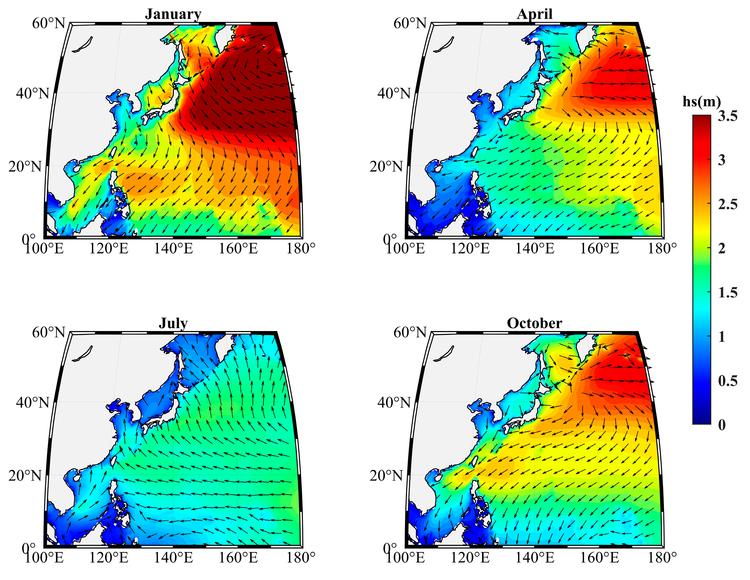
The seasonal patterns of the oceanic state of the NWP are closely linked to the seasonal patterns of monsoons, especially in the 30–60°N region. With respect to these seasonal patterns, we considered four months (January, April, July, and October, by convention) to better comprehend the NWP wave climate. The 20-year (2001–2020) averaged significant height of total waves in each of these months is shown in Figure 1. January (boreal winter) is characterized by the highest wave height in the NWP, with a mean significant wave height of total waves of 2–4 m. April (boreal spring) and October (boreal autumn) constitute transition periods, with broadly low wave heights and similar wave directions, but there are higher wave heights near Taiwan in October due to the tropical cyclone effect. July (boreal summer) has the lowest wave heights, in contrast to the wave climate during the other three seasons. The significant heights of total waves in the South China Sea and the Sea of Japan always remain low compared to the waves in the open ocean. This is due to the presence of islands that block wave propagation from the open ocean. Apart from the effect of the low-pressure systems, the waves all move onshore, especially in China’s offshore waters. Therefore, swells off the coast of China might propagate from the open ocean.
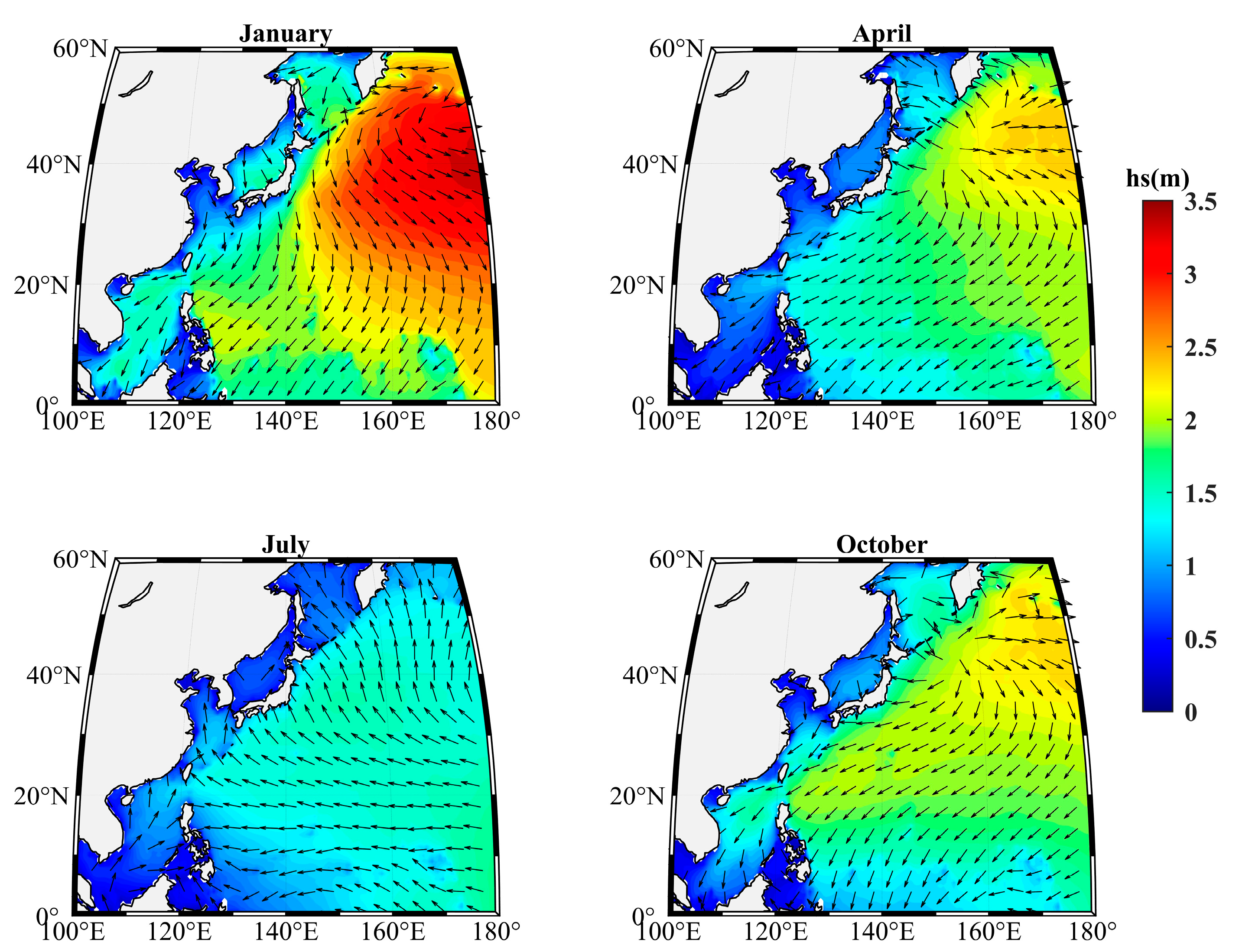
The mean significant wind sea heights and mean wind sea directions are shown in Figure 2. January (boreal winter) is characterized by seasonal wind seas in the NWP, with mean significant wind sea heights of approximately 1–3 m. April (boreal spring) and October (boreal autumn) are transition periods, exhibiting low wave heights and non-uniform wind sea directions. The lowest wind sea height occurs in July (boreal summer), with mean significant wind sea heights of <1 m in most areas of the NWP. Under the influence of tropical cyclones, typhoon waves can cause significant damage to maritime engineering and coastal engineering structures in southeastern coastal areas of China and Japan. The seasonal patterns of wind seas closely resemble those of total waves. The direction of wind seas is influenced by the prevailing wind patterns over the area where the waves are generated. For example, in areas where there are persistent westerly winds, such as in the mid-latitude extratropical storm tracks, the wind seas tend to propagate towards the east. Similarly, in areas with persistent easterly winds, such as in the trade wind belts, the wind seas propagate towards the west.
Due to their ability to carry large amounts of energy and travel over long distances, swells pose a greater threat and have a higher potential to cause significant damage than wind seas. Figure 3 illustrates the mean significant swell heights and mean swell directions. The mean significant swell heights consistently exceed the mean wind wave heights, while the directions of the swells align with those of the wind seas depicted in Figure 2. The islands located in the western part of the NWP substantially block the swells’ propagation from the open ocean to the Asian continent, especially the islands of the Philippines and Japan. Furthermore, it is also important to bear in mind that swells can carry hazardous waves over great distances. Although swells can carry more energy than wind seas, the propagation of swells is usually affected by the presence of land.
3.2. Hazardous Waves in the Northwest Pacific
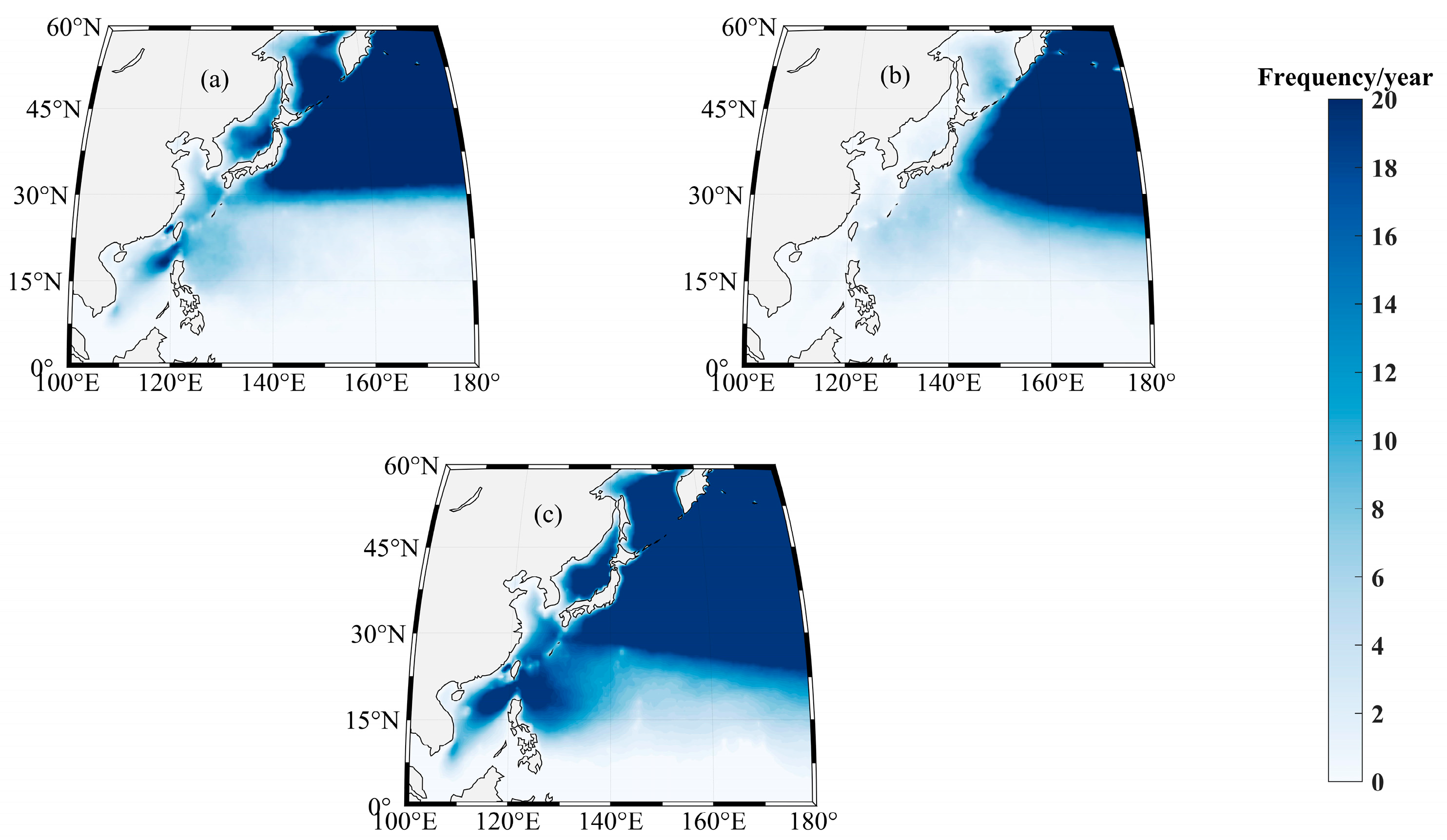
Waves with significant heights of ≥4 m pose a threat to most vessels [47]. We define these waves as hazardous waves. Figure 4 depicts the annual frequency of wave heights of ≥4 m using the daily maximum wave height derived from the hourly ERA5 dataset. This frequency represents the number of days per year on which hazardous waves occur. Figure 4a shows a visible boundary at 30°N when describing the frequency of hazardous wind seas, and the frequency in the north is higher than that in the south, which reflects the impact of large-scale low-pressure systems. In terms of the frequency of hazardous swells (Figure 4b), the boundary between the high and low frequencies is more southerly than that of the wind seas. This may be due to the transformation of wind seas into swells when the hazardous wind sea (generated by the low-pressure system in the north NWP) move southwards. Moreover, the frequency of hazardous swells is much smaller than that of hazardous wind seas in the offshore areas of Asia, such as the Sea of Okhotsk, the Sea of Japan, and the offshore areas of China, due to the existence of the offshore island chain, making it hard for hazardous swells to move into offshore areas. Figure 4c displays the frequency of total hazardous waves. Generally, low-latitude ocean areas tend to have a low frequency of hazardous waves. It is noted that there is a relatively high frequency of hazardous waves in the offshore waters of China, especially in the south and east of Taiwan island, with a value of more than 20 times per year. This phenomenon is attributed to the frequent typhoons that impact these regions multiple times each year.
In general, swells have capacity to carry more energy and travel longer distances than wind seas, but the existence of the offshore island chain makes it hard for hazardous swells to move into offshore areas. Despite the predominance of ocean swells, hazardous waves are predominantly initiated by wind seas near the eastern coast of Asia. Hazardous wind seas are mainly concentrated in the regions of the high latitudes and typhoon-affected ocean areas, and swells cause the propagation of hazardous waves across the ocean.
3.3. Extreme Wave Heights in the NWP
Extreme waves, which are usually generated by severe weather system such as tropical cyclones, are the primary cause of ocean hazards. EWH serves as a crucial point of reference in the assessment of ocean wave risk. Therefore, we analyze the EWH in this subsection in order to obtain a comprehensive understanding of the hazardous waves in the NWP. We extract the maximum value from the hourly significant wave heights of the ERA5 data as the EWH in this subsection.
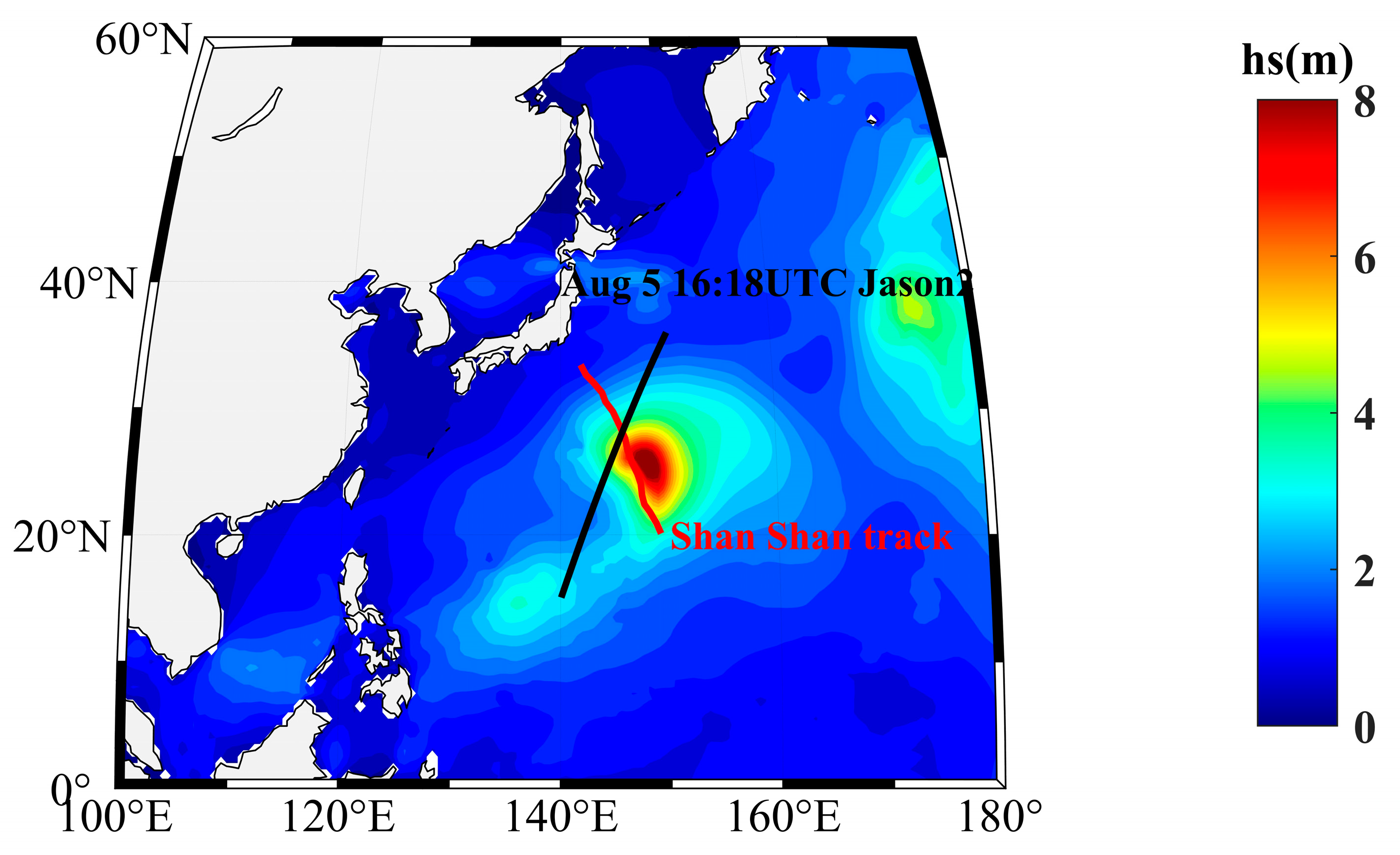
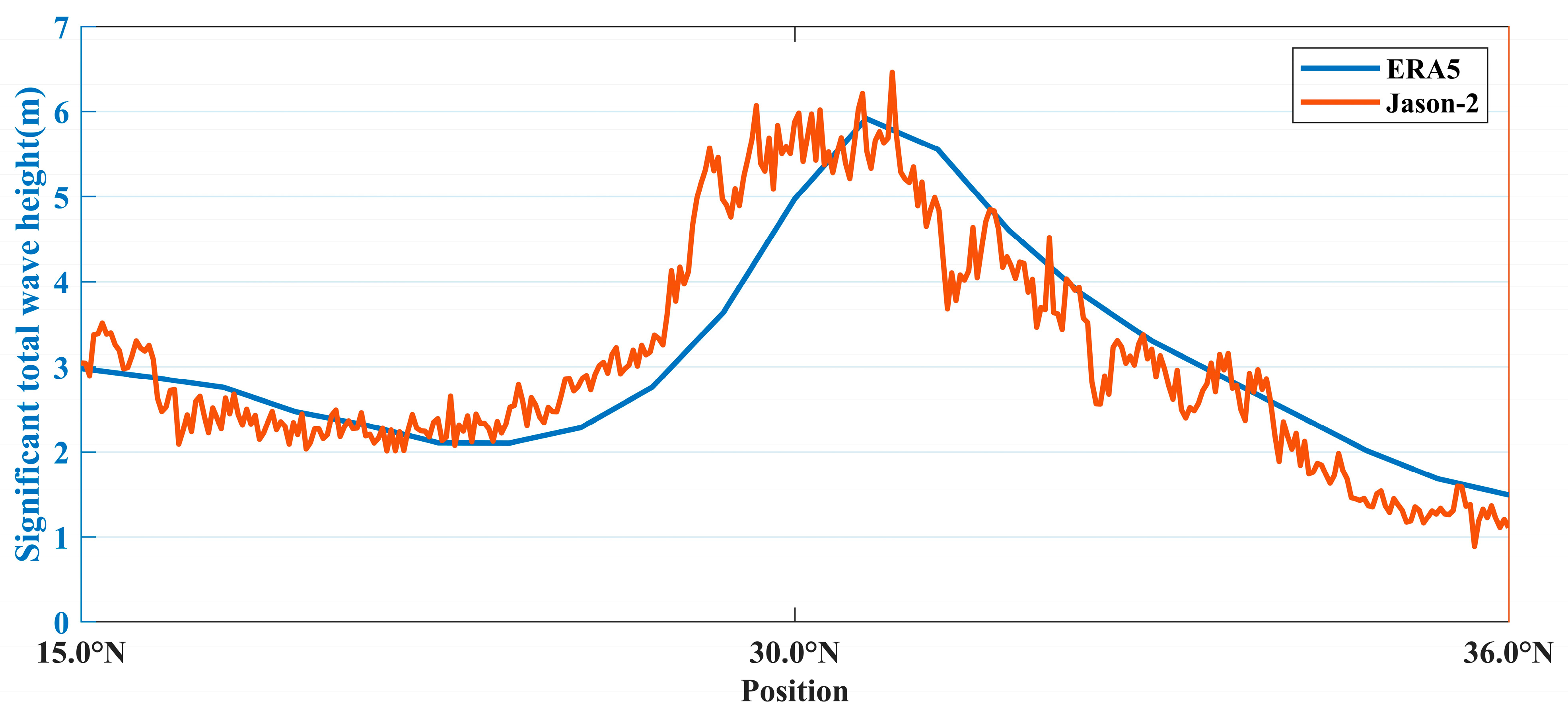
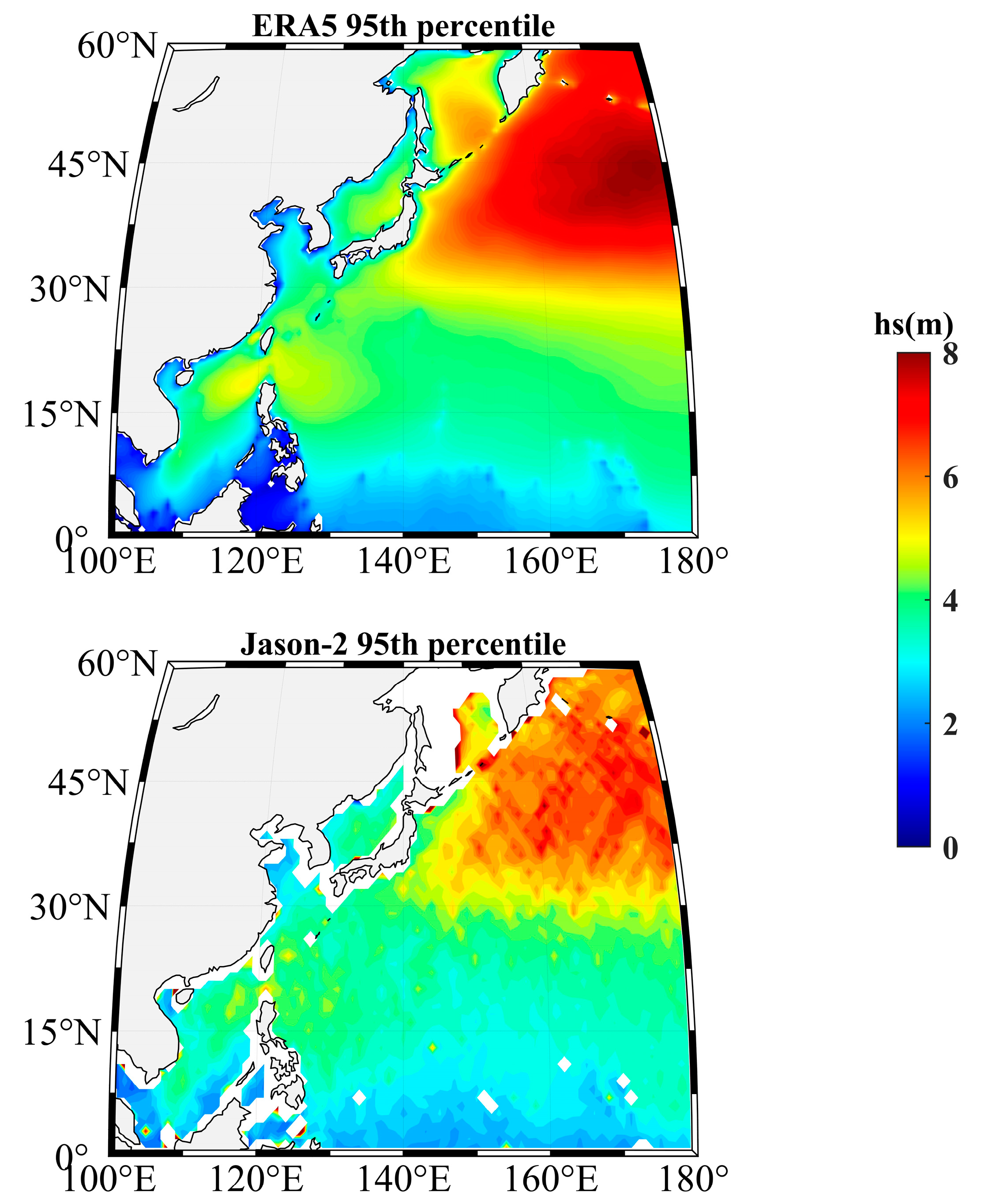
Before the estimation of the EWH, we first validated the accuracy of the ERA5 data in the context of typhoon events within the NWP using altimeter observations. We selected Typhoon Shanshan (2018) as our case study, as it was captured by the Jason-2 altimeter at about 16:18 UTC on August 5, and a complete set of observation data across Shanshan was obtained (Figure 5). Figure 6 shows the comparison of the ERA5 reanalysis data with the altimeter-observed significant wave height. The mean significant wave heights of the ERA5 and the altimeter were 3.10 m and 3.11 m, respectively, while the maximum wave heights were 5.92 m and 6.46 m, respectively. Although the mean significant wave height of the ERA5 was similar to that of Jason-2, the EWH of the ERA5 was slightly underestimated. A number of studies have also compared reanalysis model estimates of EWH with both buoy and altimeter data [26,28,48,49], showing that the model results maybe 10% lower than the buoy and altimeter data. Figure 7 illustrates the 95th percentile significant total wave height obtained from the ERA5 and Jason-2 altimeter data. Although both data sets exhibit similar magnitudes, the satellite data exhibit several gaps in coverage within the nearshore region. This was also confirmed by Jin et al. [30,50].
Since the altimeter data are discrete in time and space and cannot adequately capture the extreme waves, we use the hourly dataset of ERA5 in this paper, although there may be some deviations in the extreme value. This work can be further undertaken in the future when more comprehensive altimeter data are available.
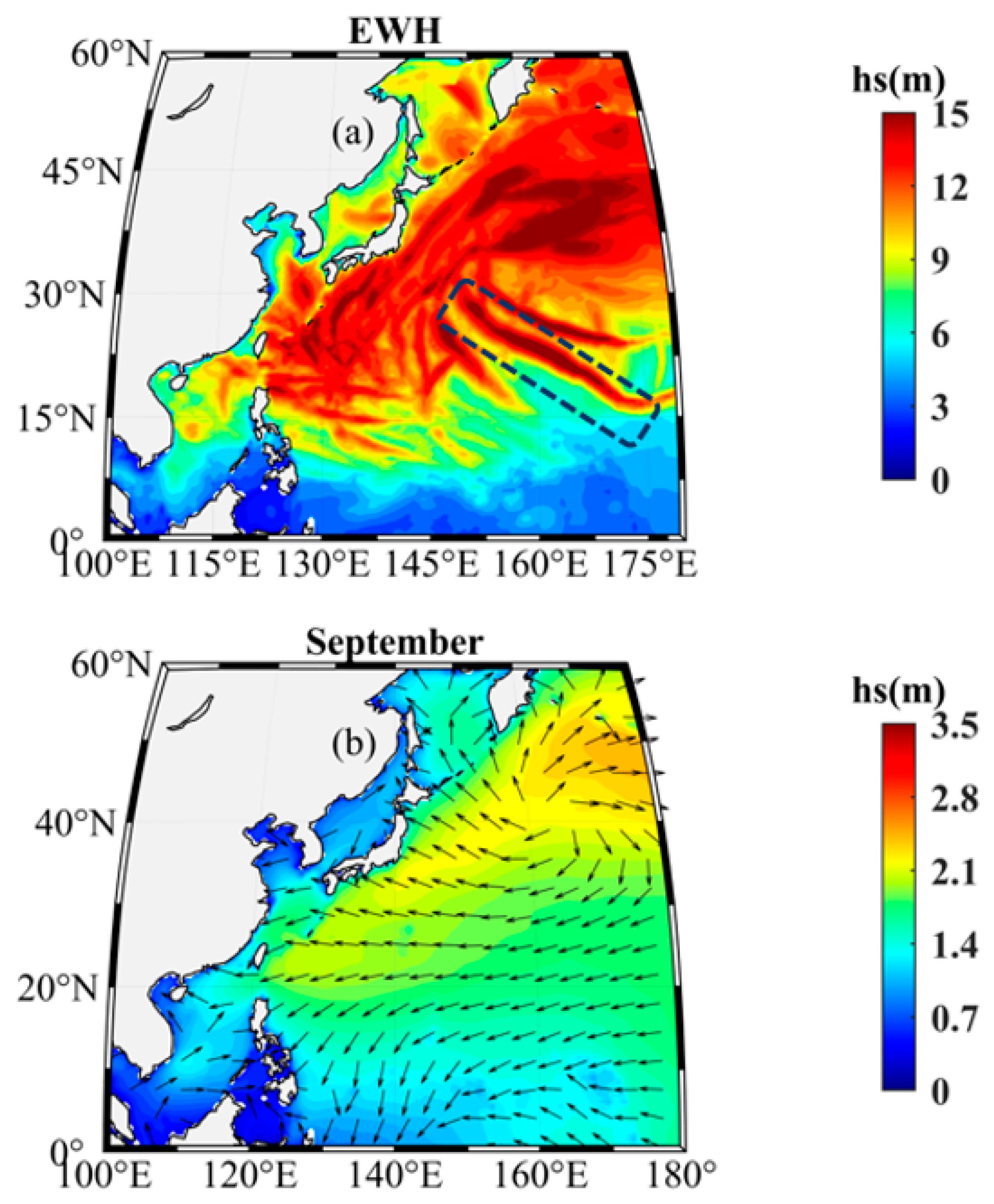
Figure 8a depicts the EWH distribution of total waves in the NWP. In addition to the EWH generated by the large-scale low-pressure systems, the distribution of EWH coincides in part with the paths of typhoons. By checking the time and location of some of the EWHs, it is known that many EWHs are caused by typhoons. Within the NWP area, the highest EWH was 18.10 m, which was observed at 23.5°N, 160.0°E on 1 September 2006. This remarkable phenomenon was caused by a tropical cyclone named Ioke (http://agora.ex.nii.ac.jp/digital-typhoon/summary/wnp/l/200612.html.en, accessed on 1 April 2023), which also set a record for the lowest atmospheric pressure in the central Pacific region, with a value of 920 hPa. The seas southeast of China and the Japanese islands are vulnerable to typhoon waves with EWH values of >10 m. Conversely, low-latitude ocean regions generally exhibit EWH values of less than 5 m in most areas.
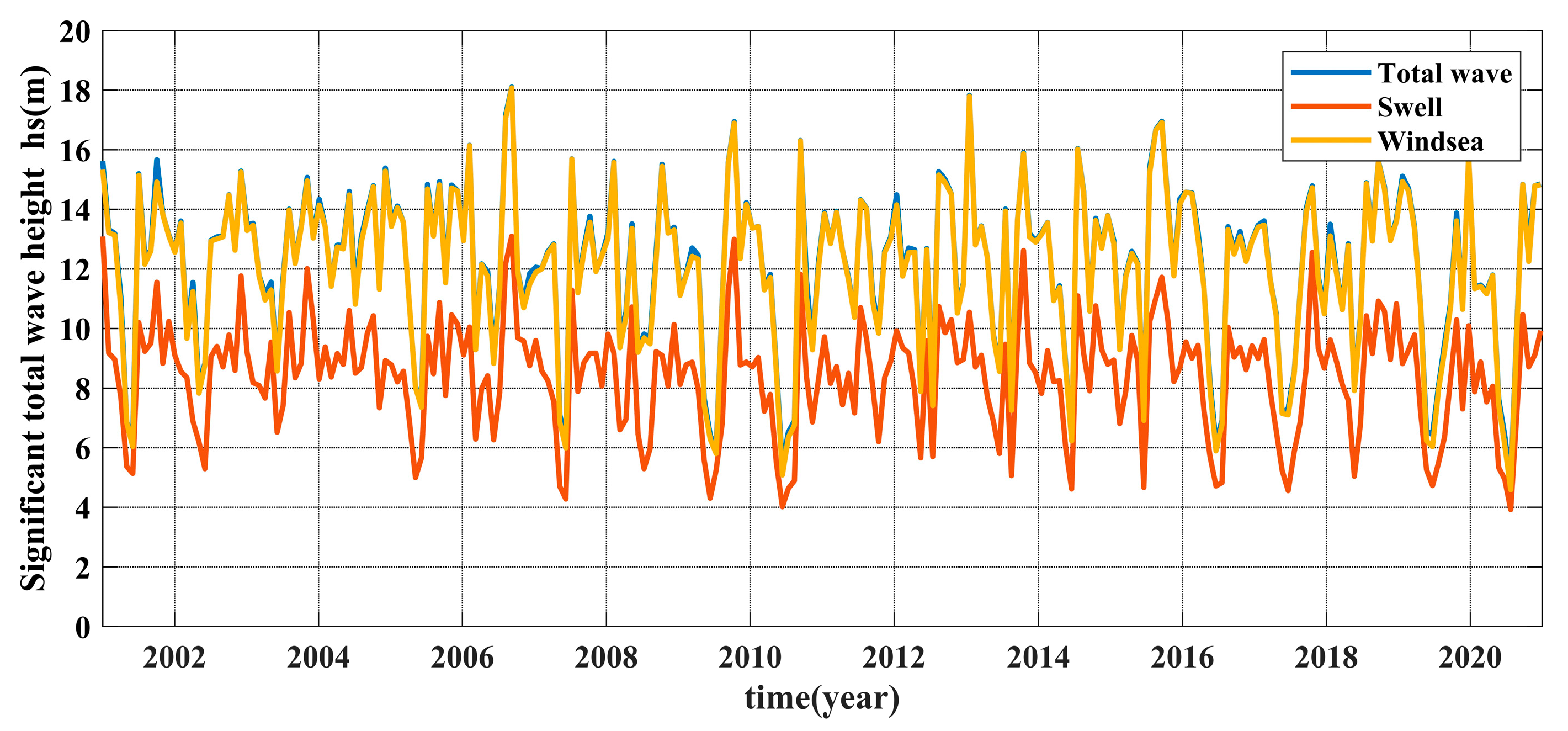
The time series of the EWH in the NWP is shown in Figure 9. The EWH calculated by total waves is broadly consistent with that calculated by wind seas, with both values being similar. The EWH of the swells is always lower than that of the total waves and the wind seas, while most of the total wave EWH values are almost equal only to the wind sea EWH. This scenario might be caused by the wave partitioning method of the wave model. The wind seas become too predominant in storm wind conditions, leading to almost the same EWH values for total waves and wind seas. The minimum EWH of total waves is 4.8 m, implying that hazardous waves have occurred every month in the NWP over the past 20 years. As depicted in Figure 8a, the highest EWH in the NWP was 18.10 m (1 September 2006), caused by the tropical cyclone Ioke. It is well known that August and September are the peak months for typhoon waves [51]. Our research also indicates that the occurrence of high waves is substantially elevated during this period, as evidenced by Figure 9. Figure 8b shows the significant heights and mean directions of total waves in September, when the western Pacific region exhibits higher waves than the central Pacific. Note that the hazardous waves generated by tropical cyclones are temporary phenomena and are not frequent in long-term statistics, so they are not clearly shown in the averaged values.
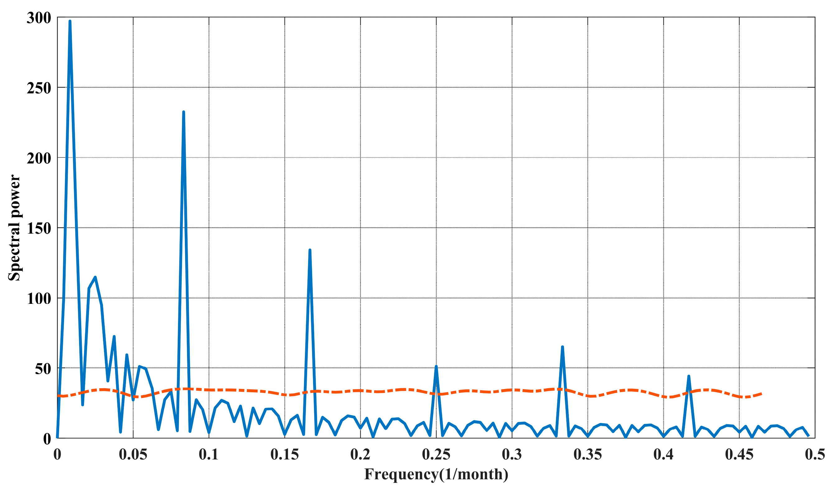
We further analyzed the period of the EWH time series using frequency spectra, as illustrated in Figure 10. The principal frequencies are 1, 0.5, and 3.3 years. Because of the monsoon climate, the temporal variation in the EWH has seasonal periodicity, such as 1 and 0.5 years. The 3.3-year period of variation may indicate the periodicity of the North Pacific Oscillation [52,53]. This implies that the occurrence of EWH may be influenced by the Aleutian Low and the Hawaiian High.
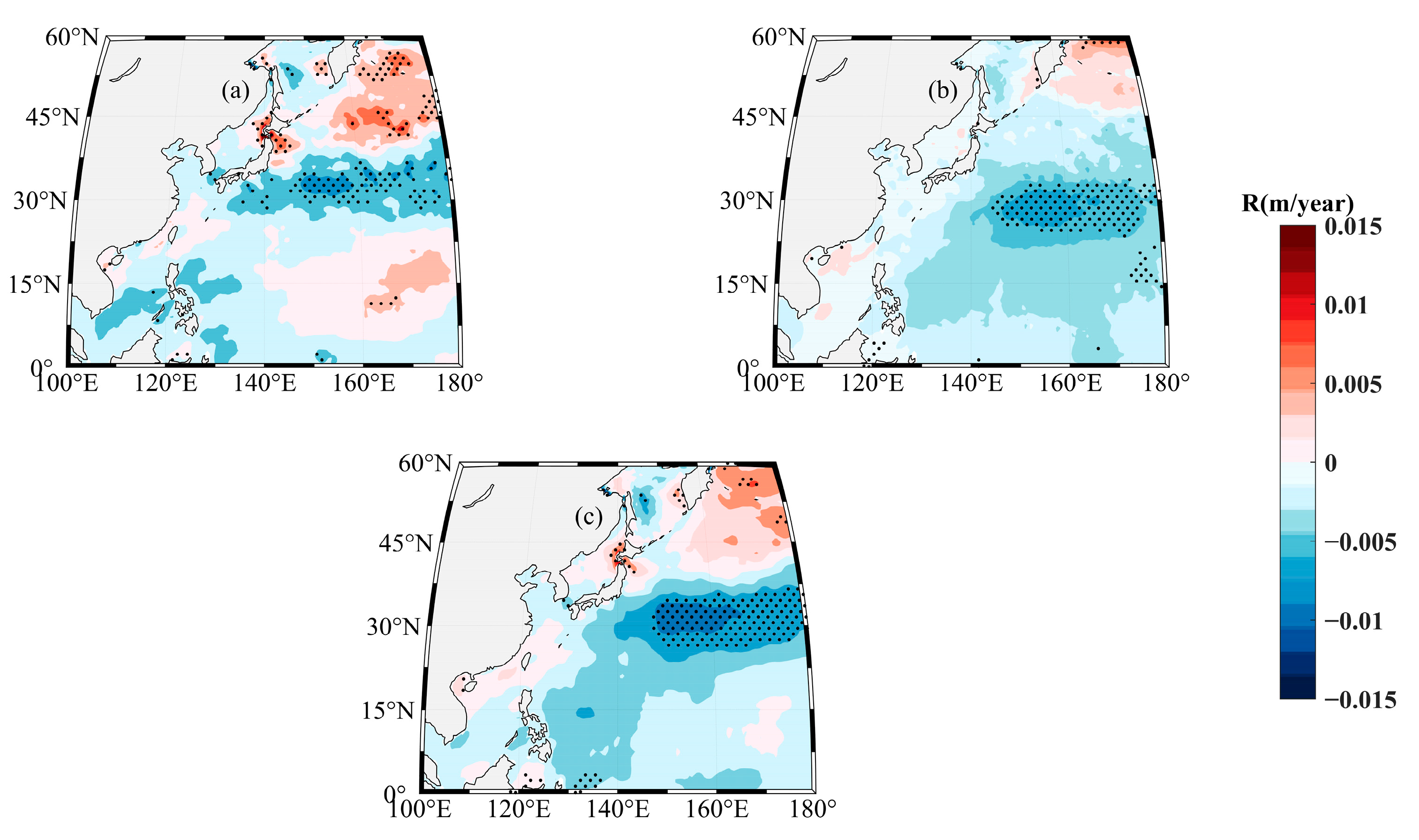
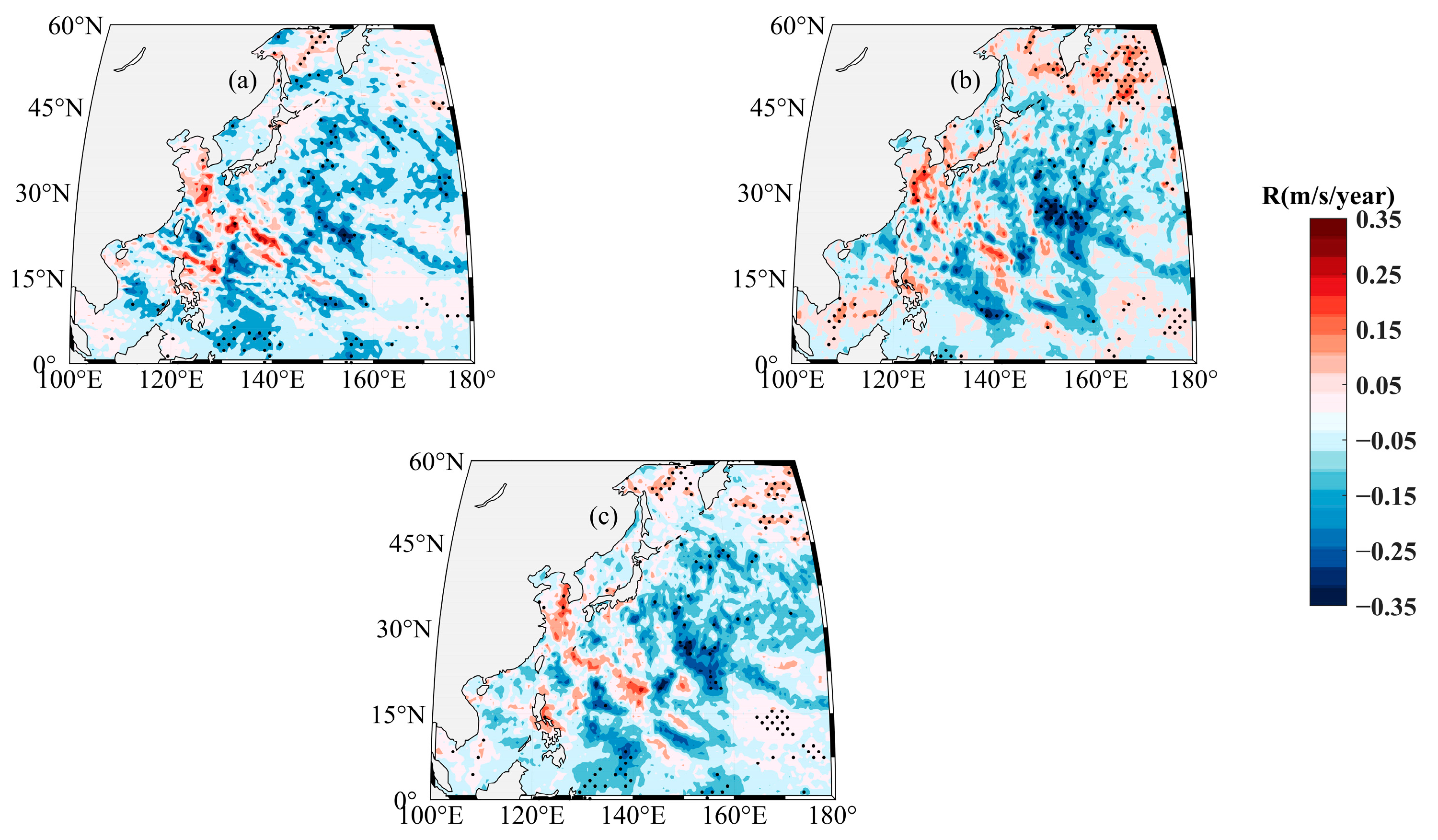
Over the past few decades, the EWH has increased globally, especially in coastal regions [9,10,11,12]. Young and Ribal found a small increase in both significant wave heights and the mean wind speed using global satellite data from 1985–2018 [10]. Figure 11 displays the distributions of the annual increase rate of the EWH in the NWP. Our analysis in Figure 11 also shows a small increase in the EWH of total waves, wind seas, and swells in the coastal regions. The annual rate of increase along the southeast Chinese coast is positive, which might reflect the impact of climate change. The frequency of the most intense tropical cyclones has increased over the past few decades [12,14], as confirmed by the annual increase rate in the EWH in the locations where tropical cyclones are generated. Apart from a negative center at 30°N, where the EWHs of both swells and wind seas are decreasing, the EWH shows an increasing trend in high- and low-latitude ocean areas. There is a maximum rate of increase of the extreme total wave height in the region of the Japanese archipelago, with a value of 0.013 m/year (Figure 11c), which is caused by an increase in EWH of wind seas, according to Figure 12a. The extreme wind speed in the south of Japan shows an increasing trend due to the frequency of intense tropical cyclones, which has increased over the past few decades. However, this trend is not reflected in the EWH. A possible reason for this is that the ERA5 data underestimate the EWH, so the increasing rate of EWH caused by typhoons is not significant in typhoon-prone regions. Figure 12 depicts the annual increase rate of extreme wind speeds. The spatial distribution of the annual increase rate in wind seas, as shown in Figure 12a, closely resembles that of the wind speeds in Figure 12c. Additionally, according to Figure 12b,c, changes in meridional wind speeds is the primary reason for the change in total wind speed over the past 20 years.
4. Discussion
In this section, we discuss the risk assessment of hazardous ocean waves, which is crucial to understanding ocean wave disasters and is highly important for government officials and other decision-makers conducting damage assessments or economic loss analyses. The wave intensity level, the wave risk index, the wave risk level, and the 50-year and 100-year return periods of EWH are used to assess the risk of wave disasters in the NWP from different perspectives.
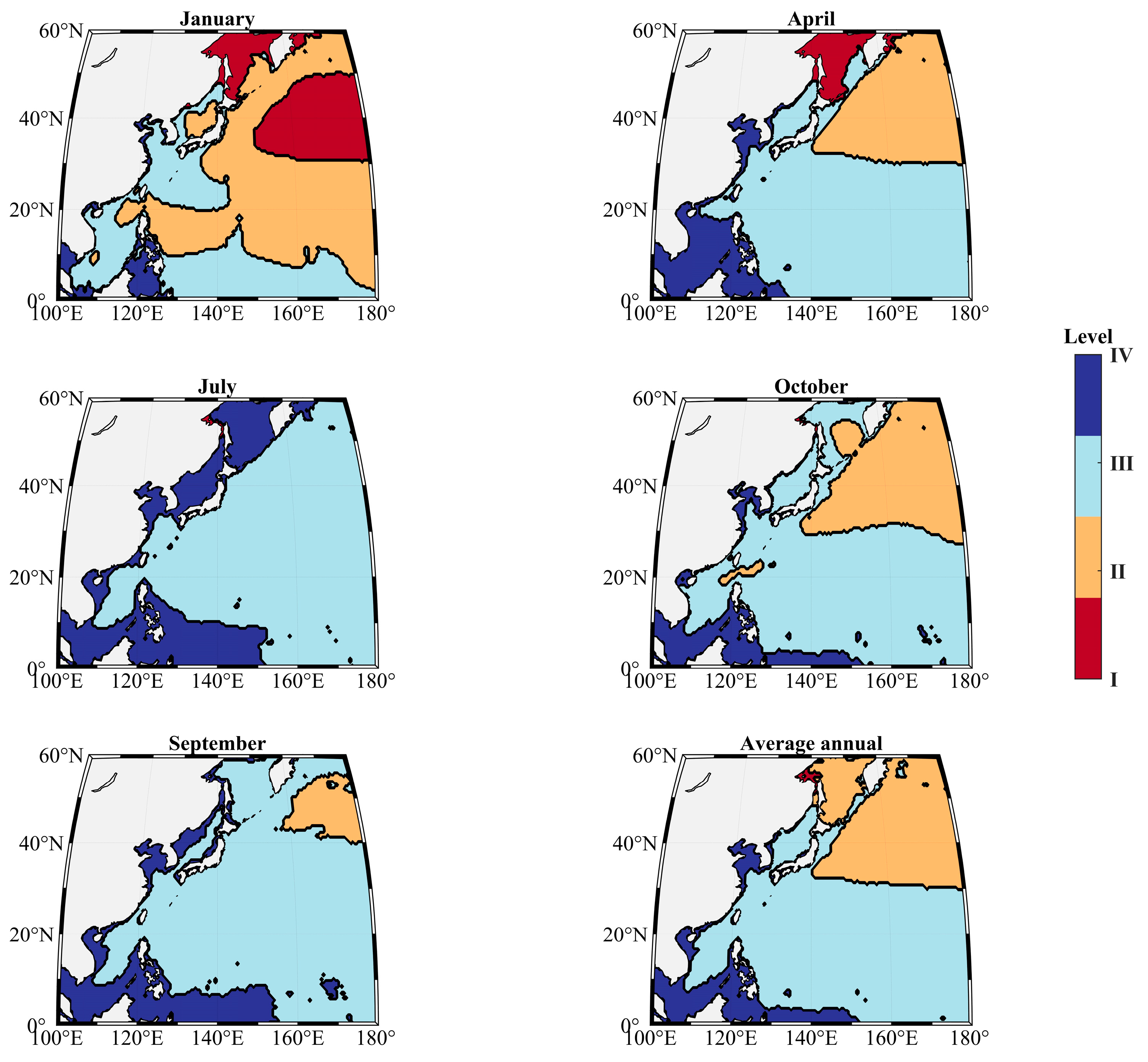
Figure 13 shows the seasonal variation in wave intensity according to Table 1, calculated from the daily maximum wave heights averaged over 20 years. During winter, the NWP experiences higher levels (i.e., levels I and II) throughout most of the area; meanwhile, in summer, the wave intensity is at level III or IV across the entire NWP. The Sea of Okhotsk has level I wave intensity when not covered by sea ice in winter and spring. The wave intensity in the offshore waters of China and low-latitude ocean areas (except in the area around Taiwan Island) experience low levels throughout the year. In particular, the low latitude of the eastern Pacific has been at the lowest wave intensity throughout the period under consideration. In October, a center of level II intensity occurs near Taiwan, due to the effects of tropical cyclones. The 30°N dividing line is visible in April and October; this is the line that demarcates the large-scale low-pressure system. Overall, wave intensity is highest in January (boreal winter) and the level I wave intensity occupies the largest area compared to the other three seasons. Although typhoons are frequent in September, no significant increase in wave intensity occurs due to the average value used in the calculations.
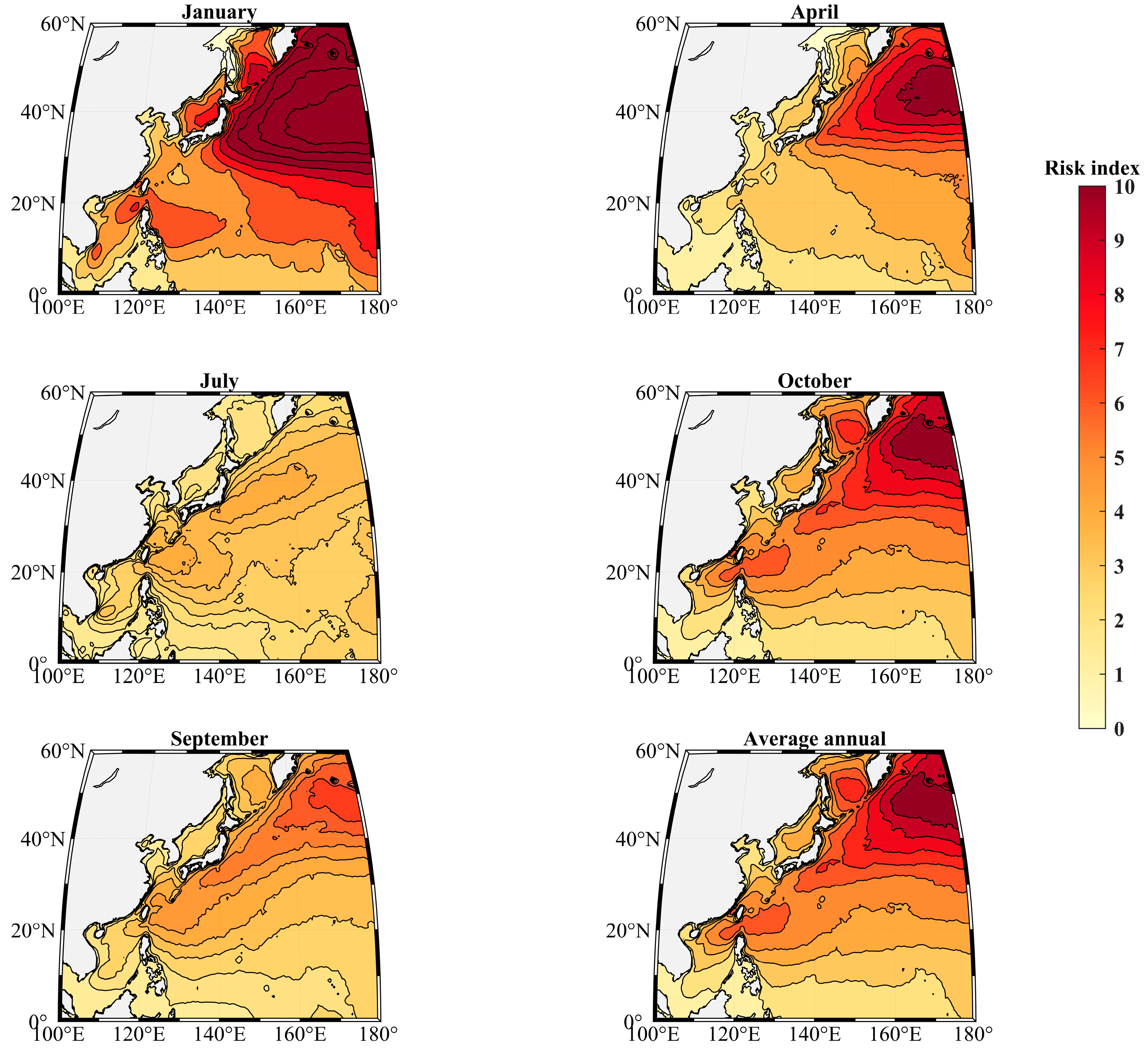
It is insufficient to rely solely on the maximum daily wave heights to reflect wave hazards, as persistent small waves have the potential to continuously inflict damage upon coastal structures. Therefore, it is imperative to ascertain the wave hazard by affording suitable weightage to each wave intensity. The distribution of the ocean wave risk index , calculated using Equation (9), is shown in Figure 14. The large-scale low-pressure systems cause the highest risk index in winter, and the risk index becomes smaller toward lower latitudes. In the zonal direction, the risk index becomes smaller toward the west because the prevailing wave direction is eastward under the influence of the large-scale low-pressure systems. During July, although the wave intensity is at level III in most ocean areas, the regions off the east coast of China and off the east coast of the Japanese Archipelago have higher ocean wave risk index values. During autumn, owing to the effect of tropical cyclones, Taiwan and the Japanese Archipelago have higher ocean wave risk index values, as shown by the findings derived from Figure 13. Furthermore, it can be observed that the level of wave risk along the coastal areas of China in the months of January and September is relatively elevated, albeit for varying reasons, as delineated in Figure 1 and Figure 8, which depict the prevailing wave directions.
Compared with wave intensity, more details can be observed through the risk index shown in Figure 14. The risk index shows a higher distribution along both the east China Sea and the waters of the eastern Japanese Archipelago. However, the effect of temporary hazard waves, such as typhoon waves, is still weakened in the calculation of the average risk index. Overall, the distribution of wave intensity does not necessarily represent the distribution of risk illustrated by the wave risk index.
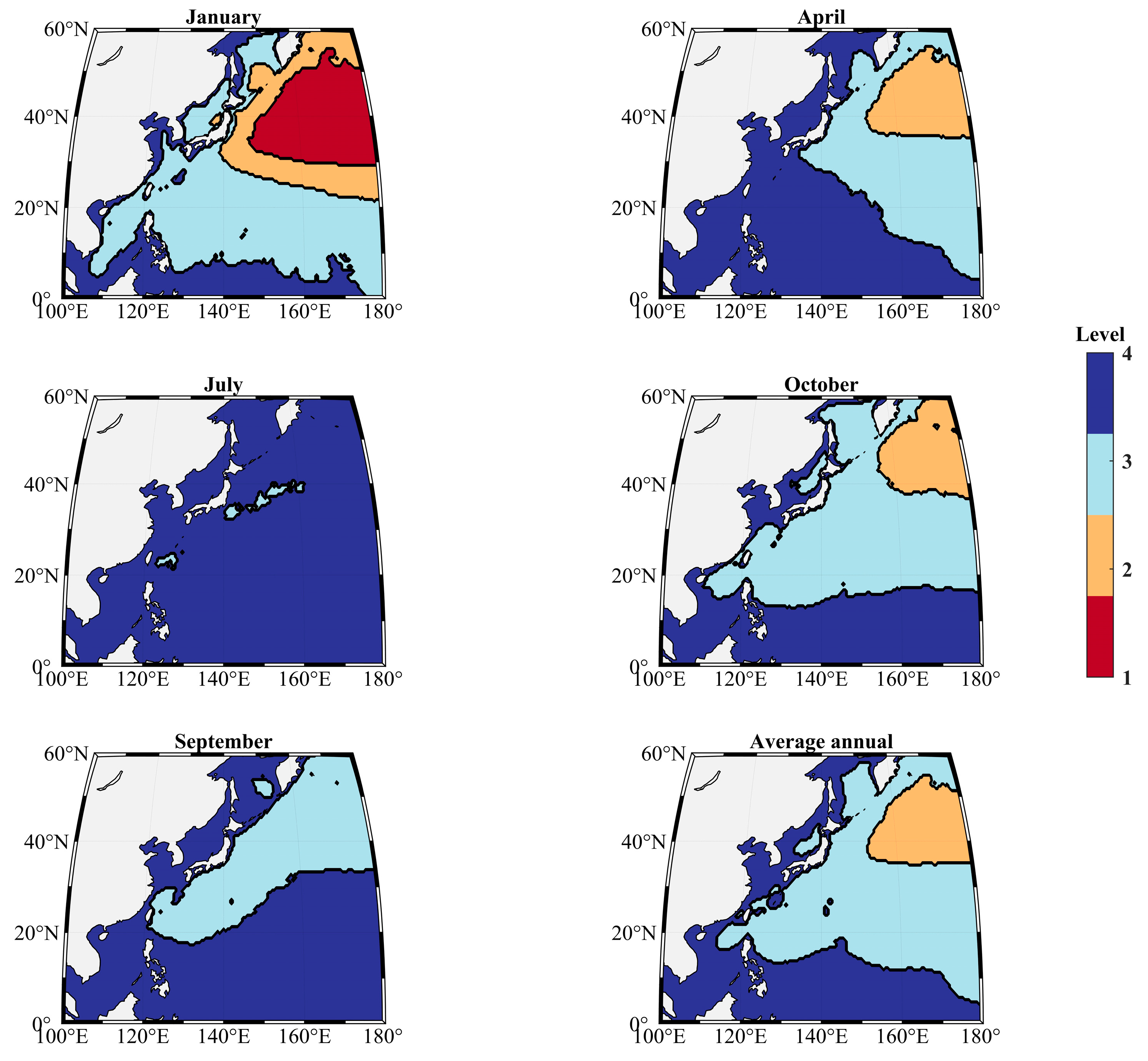
We utilized to represent the normalized risk index to determine the wave risk level at each grid point. The corresponding classification can be found in Table 2. Figure 15 displays the distribution of the normalized wave risk level. Level 1 indicates that waves are highly likely to cause damage, while level 4 suggests the minimal destructive potential of the waves. During winter, the entire NWP experiences the highest danger level, with level 1 even appearing in the high-latitude regions. In summer, level 4 dominates most of the NWP. However, tropical cyclones begin to affect the waves in the NWP during this season. Level 3 is observed to the east of Taiwan and to the east of the Japanese Archipelago, a finding similar to that derived from Figure 13. In July, October, and September, tropical cyclones give rise to varying risk levels near the southeastern coast of Asia. It is worth noting that the wave risk level at high latitudes decreases due to decreases in the wave heights.
The spatial distribution of the wave risk levels shows rougher information compared to the wave risk index in Figure 14, although their overall trend is the same. The distributions of the wave intensity levels and risk levels are also generally similar. However, the range of higher wave intensity levels is greater than the range of wave risk levels, except for areas controlled by low-pressure systems in January. This is possibly because the wave intensity level is vulnerable to extreme waves, but the wave risk level considers the effects of all waves. As such, the different assessment methods exhibit slightly different distributions. However, while all three of these methods can be used to assess hazardous waves, none of them can visualize the magnitude of the wave height.
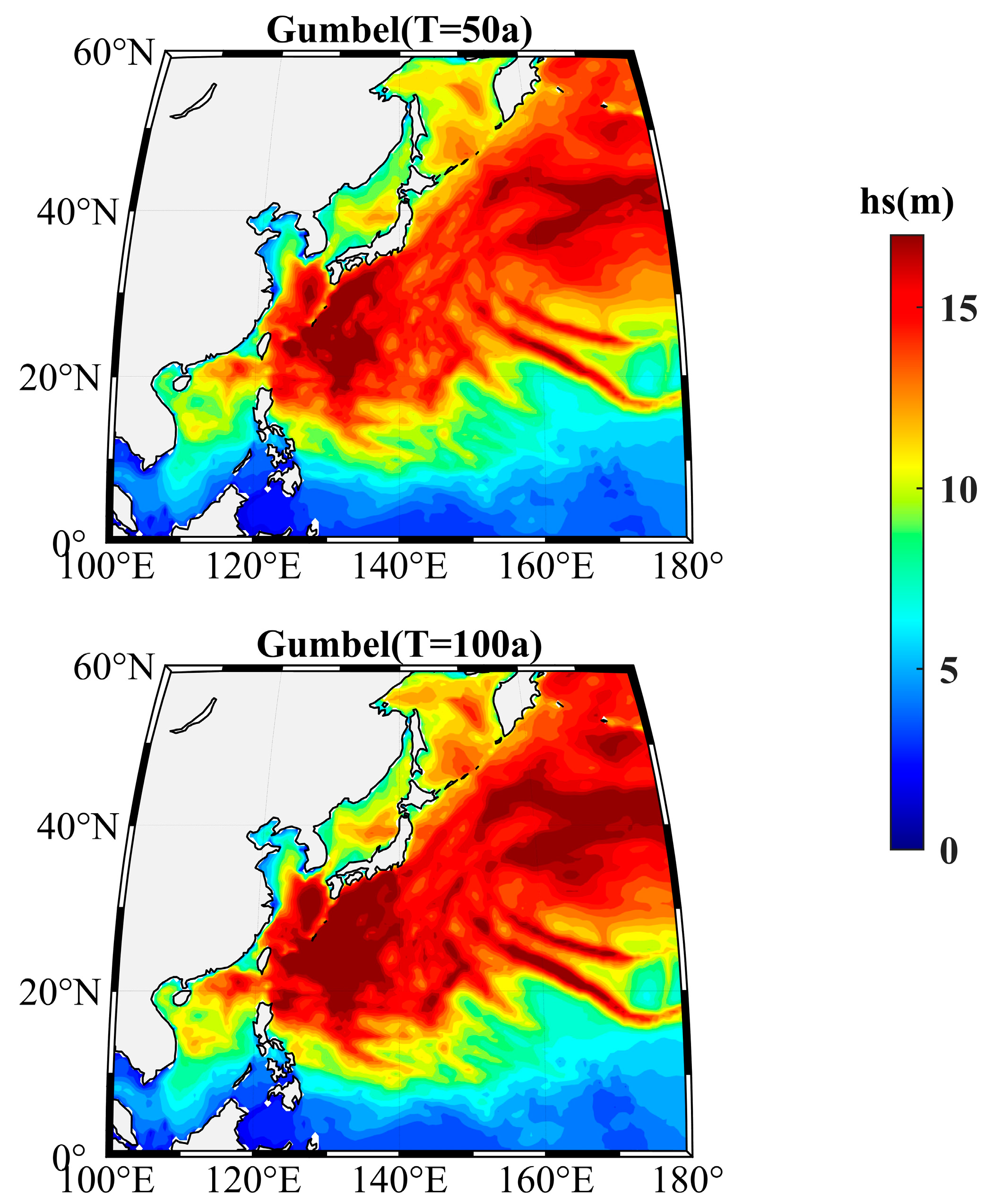
It is necessary to investigate the EWHs for the 50-year and 100-year return periods when studying wave hazards. Through the utilization of the Gumbel distribution approach, we calculated the EWHs for the 50-year and 100-year return periods, as shown in Figure 16. As opposed to the assessment methods used for hazardous waves, the return period has the distinct advantage of accurately determining the impact of extreme waves, notably those generated by typhoons. It is worth noting that, as well as regions influenced by large-scale low-pressure systems, typhoon-affected areas in the western Pacific Ocean also show large EWH values for the 50-year and 100-year return periods. The highest EWH values are 20.92 and 23.07 m for the 50-year and 100-year return periods in the NWP, respectively. If 10% bias is considered, the highest EWH values are 23.01 and 25.38 m. The EWH distribution pattern (Figure 16) resembles that which is exhibited in Figure 8a, and it is prone to influence from typhoon waves, particularly in the western Pacific Ocean. Significantly, the tails of the EWH distribution echo the trajectory of typhoons, as evidenced by a notable emergence of EWH clusters in the central Pacific Ocean. Although the risk level is not high along the coast of China, as shown in Figure 15, an offshore EWH of up to 15 m can still prove disastrous. Therefore, offshore areas should pay attention to the potential for disasters caused by typhoon waves. Finally, analyses indicate that the ocean areas situated in low-latitude zones tend to exhibit low wave heights. However, the return period is strongly influenced by occasional extreme weather, which can adversely affect the assessment of long-term variability in wave hazards. Therefore, a single research method cannot be used for the study of wave hazards.
5. Conclusions
The NWP Warm Pool is one of the main sources for typhoon generation, and approximately 25% of the typhoons generated in this region can affect offshore areas of China. The monsoon climate of the NWP also causes hazardous waves in offshore areas. As such, this study investigated the statistical features of hazardous waves in the NWP over the period from 2001–2020, using hourly ERA5 reanalysis data.
Based on the various characteristics of swells and wind seas, we examined the EWH values of wind seas and swells separately. Although hazardous wind seas occur more frequently than hazardous swells, swells can cause hazardous waves to travel further. They are also an important factor in wave hazards. Our research indicates that tropical cyclones in the NWP region are another factor responsible for generating EWH, a phenomenon that is temporary and not prominently reflected in long-term statistical trends. However, this study underscores that the hazardous waves caused by typhoons are not readily perceptible when examining the seasonal variation. Additionally, we identified that the occurrence of extreme waves has a 3.3-year period. Owing to the increase in tropical cyclones associated with climate change, the EWH has also increased in the offshore waters of China over the past 20 years. This increase is primarily attributable to the changes in the meridional wind speed. Then, we graded the wave intensity and wave hazard level according to the significant height of total waves, and the different classification methods produced different results. Moreover, we also calculated the long-term return period of EWH, and discovered that an EWH with a 100-year return period can reach up to 23.07 m. The comparisons of mean wave height between the ERA5 and altimeter data show good agreement, while ERA5 underestimates the EWH. Therefore, the long-term return period of EWH could also be underestimated in this article. However, the ERA5 data exhibit remarkable consistency in both the temporal and spatial dimensions, and they separates out swells and wind seas. Overall, the ERA data can be relied upon as a reliable source of information for statistical analysis and research.
The present investigation may offer valuable insights into the development of the marine economy (including maritime shipping and fishing operations) and ocean engineering structures. While the ERA5 dataset displays precision in estimating the EWH and integrating observational data, insufficiencies in the spatial resolution may persist. To address this, wave models with high spatial resolution can be utilized to explore potential wave hazards in greater detail in the future.
Author Contributions
Conceptualization, R.L. and W.Z.; formal analysis, K.W.; funding acquisition, W.Z. and K.W.; investigation, X.D.; methodology, L.L.; project administration, W.Z.; resources, K.W.; validation, K.W. and R.L.; Visualization, W.Z. and J.L.; writing—original draft, R.L. and S.L.; writing—review and editing, A.V.B., R.L. and W.Z. All authors have read and agreed to the published version of the manuscript.
Funding
This research was funded by the National Natural Science Foundation of China under grant numbers 42176018 and U20A2099.
Data Availability Statement
The data used in this study are available at https://cds.climate.copernicus.eu/cdsapp#!/dataset/reanalysis-era5-single-levels?tab=form (accessed on 1 April 2023). The significant wave heights derived from Jason-2 were downloaded from the Australian Ocean Data Network (AODN) portal (http://portal.aodn.org au/search, accessed on 1 April 2023) [38]. Data were sourced from Australia’s Integrated Marine Observing System (IMOS); IMOS is enabled by the National Collaborative Research Infrastructure strategy (NCRIS).
Acknowledgments
The authors thank the researchers who obtained and published the data and schemes used in this study. R.L. acknowledges the fellowship provided by the China Scholarship Council (CSC:202206330001). S.L. and A.V.B. acknowledge support from the U.S. Office of Naval Research Grant N62909-20-1-2080.
Conflicts of Interest
The authors declare no conflict of interest.
References
- Munk, W.H.; Miller, G.R.; Snodgrass, F.E.; Barber, N.F. Directional recording of swell from distant storms. Philos Trans. R. Soc. London. Ser. A Math. Phys. Sci. 1997, 255, 505–584. [Google Scholar] [CrossRef] [PubMed]
- Li, R.; Wu, K.; Li, J.; Dong, X.; Sun, J.; Zhang, W.; Liu, Q. Relating a Large-Scale Variation of Waves in the Indian Ocean to the IOD. J. Geophys. Res. Oceans 2022, 127, e2022JC018941. [Google Scholar] [CrossRef]
- Li, R.; Wu, K.; Li, J.; Akhter, S.; Dong, X.; Sun, J.; Cao, T. Large-Scale Signals in the South Pacific Wave Fields Related to ENSO. J. Geophys. Res. Oceans 2021, 126, e2021JC017643. [Google Scholar] [CrossRef]
- Chen, G.; Chapron, B.; Ezraty, R.; Vandemark, D. A global view of swell and wind sea climate in the ocean by satellite altimeter and scatterometer. J. Atmos. Ocean. Technol. 2002, 19, 1849–1859. [Google Scholar] [CrossRef]
- Semedo, A.; Sušelj, K.; Rutgersson, A.; Sterl, A. A Global View on the Wind Sea and Swell Climate and Variability from ERA-40. J. Clim. 2011, 24, 1461–1479. [Google Scholar] [CrossRef]
- Zhang, Z.; Li, X.-M. Global ship accidents and ocean swell-related sea states. Nat. Hazards Earth Syst. Sci. 2017, 17, 2041–2051. [Google Scholar] [CrossRef]
- Walsh, K.J.E.; Camargo, S.J.; Knutson, T.R.; Kossin, J.; Lee, T.C.; Murakami, H.; Patricola, C. Tropical cyclones and climate change. Trop. Cyclone Res. Rev. 2019, 8, 240–250. [Google Scholar] [CrossRef]
- Webster, P.J.; Holland, G.J.; Curry, J.A.; Chang, H.R. Changes in tropical cyclone number, duration, and intensity in a warming environment. Science. 2005, 309, 1844–1846. [Google Scholar] [CrossRef]
- Ruggiero, P.; Komar, P.D.; Allan, J.C. Increasing wave heights and extreme value projections: The wave climate of the U.S. Pacific Northwest. Coast. Eng. 2010, 57, 539–552. [Google Scholar] [CrossRef]
- Young, I.R.; Ribal, A. Multiplatform evaluation of global trends in wind speed and wave height. Science 2019, 364, 548–552. [Google Scholar] [CrossRef]
- Young, I.R.; Zieger, S.; Babanin, A.V. Global trends in wind speed and wave height. Science 2011, 332, 451–455. [Google Scholar] [CrossRef] [PubMed]
- Allan, J.; Komar, P. Are ocean wave heights increasing in the eastern North Pacific? Eos Trans. Am. Geophys. Union 2000, 81b, 561–567. [Google Scholar] [CrossRef]
- Liu, J.; Meucci, A.; Liu, Q.; Babanin, A.V.; Ierodiaconou, D.; Young, I.R. The wave climate of Bass Strait and South-East Australia. Ocean Model. 2022, 172, 101980. [Google Scholar] [CrossRef]
- Carter, D.J.T.; Challenor, P.G. Estimating return values of environmental parameters. Q. J. R. Meteorol. Soc. 1981, 107, 259–266. [Google Scholar] [CrossRef]
- Méndez, F.J.; Menéndez, M.; Luceño, A.; Losada, I.J. Estimation of the long-term variability of extreme significant wave height using a time-dependent Peak Over Threshold (POT) model. J. Geophys. Res. 2006, 111. [Google Scholar] [CrossRef]
- Menéndez, M.; Méndez, F.J.; Losada, I.J.; Graham, N.E. Variability of extreme wave heights in the northeast Pacific Ocean based on buoy measurements. Geophys. Res. Lett. 2008, 35. [Google Scholar] [CrossRef]
- Sartini, L.; Cassola, F.; Besio, G. Extreme waves seasonality analysis: An application in the Mediterranean Sea. J. Geophys. Res. Ocean. 2015, 120, 6266–6288. [Google Scholar] [CrossRef]
- Alves, J.H.G.; Young, I.R. On estimating extreme wave heights using combined Geosat, Topex/Poseidon and ERS-1 altimeter data. Appl. Ocean. Res. 2003, 25, 167–186. [Google Scholar] [CrossRef]
- Wimmer, W.; Challenor, P.; Retzler, C. Extreme wave heights in the North Atlantic from Altimeter Data. Renew. Energy 2006, 31, 241–248. [Google Scholar] [CrossRef]
- Izaguirre, C.; Mendez, F.J.; Menendez, M.; Luceño, A.; Losada, I.J. Extreme wave climate variability in southern Europe using satellite data. J. Geophys. Res. 2010, 115. [Google Scholar] [CrossRef]
- Izaguirre, C.; Méndez, F.J.; Menéndez, M.; Losada, I.J. Global extreme wave height variability based on satellite data. Geophys. Res. Lett. 2011, 38. [Google Scholar] [CrossRef]
- Young, I.R.; Vinoth, J. Global Estimates of Extreme Wind Speed and Wave Height. J. Clim. 2011, 24, 1647–1665. [Google Scholar]
- Young, I.R.; Vinoth, J.; Zieger, S.; Babanin, A.V. Investigation of trends in extreme value wave height and wind speed. J. Geophys. Res. Oceans 2012, 117. [Google Scholar] [CrossRef]
- Wang, X.L.; Swail, V.R. Changes of Extreme Wave Heights in Northern Hemisphere Oceans and Related Atmospheric Circulation Regimes. J. Clim. 2001, 14, 2204–2221. [Google Scholar] [CrossRef]
- Cañellas, B.; Orfila, A.; Méndez, F.J.; Menéndez, M.; Gómez-Pujol, L.; Tintoré, J. Application of a POT Model to Estimate the Extreme Significant Wave Height Levels around the Balearic Sea (Western Mediterranean). J. Coast. Res. 2007, 329–333. [Google Scholar]
- Meucci, A.; Young, I.R.; Breivik, Ø. Wind and Wave Extremes from Atmosphere and Wave Model Ensembles. J. Clim. 2018, 31, 8819–8842. [Google Scholar] [CrossRef]
- Gao, H.; Shao, Z.; Wu, G.; Li, P. Study of Directional Declustering for Estimating Extreme Wave Heights in the Yellow Sea. J. Mar. Sci. Eng. 2020, 8, 326. [Google Scholar] [CrossRef]
- Takbash, A.; Young, I. Long-Term and Seasonal Trends in Global Wave Height Extremes Derived from ERA-5 Reanalysis Data. J. Mar. Sci. Eng. 2020, 8, 1015. [Google Scholar] [CrossRef]
- Liu, J.; Meucci, A.; Young, I.R. Projected wave climate of Bass Strait and south-east Australia by the end of the twenty-first century. Clim. Dyn. 2022, 60, 393–407. [Google Scholar] [CrossRef]
- Liu, J.; Meucci, A.; Young, I.R. Projected 21st Century Wind-Wave Climate of Bass Strait and South-East Australia: Comparison of EC-Earth3 and ACCESS-CM2 Climate Model Forcing. J. Geophys. Res. Ocean. 2023, 128, e2022JC018996. [Google Scholar] [CrossRef]
- He, H.; Song, J.; Bai, Y.; Xu, Y.; Wang, J.; Bi, F. Climate and extrema of ocean waves in the East China Sea. Sci. China Earth Sci. 2018, 61, 980–994. [Google Scholar] [CrossRef]
- Tochimoto, E.; Niino, H. Comparing Frontal Structures of Extratropical Cyclones in the Northwestern Pacific and Northwestern Atlantic Storm Tracks. Mon. Weather. Rev. 2022, 150, 369–392. [Google Scholar] [CrossRef]
- Woo, H.-J.; Park, K.-A. Estimation of Extreme Significant Wave Height in the Northwest Pacific Using Satellite Altimeter Data Focused on Typhoons (1992–2016). Remote Sens. 2021, 13, 1063. [Google Scholar] [CrossRef]
- Kang, D.; Ko, K.; Huh, J. Determination of extreme wind values using the Gumbel distribution. Energy 2015, 86, 51–58. [Google Scholar] [CrossRef]
- Hersbach, H.; Bell, B.; Berrisford, P.; Hirahara, S.; Horányi, A.; Muñoz-Sabater, J.; Nicolas, J.; Peubey, C.; Radu, R.; Schepers, D.; et al. The ERA5 global reanalysis. Q. J. R. Meteorol. Soc. 2020, 146, 1999–2049. [Google Scholar] [CrossRef]
- Dee, D.P.; Uppala, S.M.; Simmons, A.J.; Berrisford, P.; Poli, P.; Kobayashi, S.; Andrae, U.; Balmaseda, M.A.; Balsamo, G.; Bauer, P.; et al. The ERA-Interim reanalysis: Configuration and performance of the data assimilation system. Q. J. R. Meteorol. Soc. 2011, 137, 553–597. [Google Scholar] [CrossRef]
- K Bhaskaran, P.; Gupta, N.; K Dash, M. Wind-wave Climate Projections for the Indian Ocean from Satellite Observations. J. Mar. Sci. Res. Dev. 2014, 1. [Google Scholar] [CrossRef]
- Semedo, A.; Sušelj, K.; Rutgersson, A. Variability of Wind Sea and Swell Waves in the North Atlantic Based on ERA-40 Re-analysis. In Proceedings of the Eighth European Wave and Tidal Energy Conference, Uppsala, Sweden, 7–11 September 2009. [Google Scholar]
- Ribal, A.; Young, I.R. 33 years of globally calibrated wave height and wind speed data based on altimeter observations. Sci. Data 2019, 6, 77. [Google Scholar] [CrossRef]
- Fisher, R.A.; Tippett, L.H.C. Limiting forms of the frequency distribution of the largest or smallest member of a sample. Math. Proc. Camb. Philos. Soc. 2008, 24, 180–190. [Google Scholar] [CrossRef]
- Jenkinson, A.F. The frequency distribution of the annual maximum (or minimum) values of meteorological elements. Q. J. R. Meteorol. Soc. 1955, 81, 158–171. [Google Scholar] [CrossRef]
- Coles, S. An Introduction to Statistical Modeling of Extreme Values; Springer: Berlin/Heidelberg, Germany, 2001. [Google Scholar] [CrossRef]
- Kochanek, K.; Renard, B.; Arnaud, P.; Aubert, Y.; Lang, M.; Cipriani, T.; Sauquet, E. A data-based comparison of flood frequency analysis methods used in France. Nat. Hazards Earth Syst. Sci. 2014, 14, 295–308. [Google Scholar] [CrossRef]
- Ercelebi, S.G.; Toros, H. Extreme Value Analysis of Istanbul Air Pollution Data. CLEAN—Soil, Air, Water 2009, 37, 122–131. [Google Scholar] [CrossRef]
- Jain, R.K. Entrepreneurial Competencies: A Meta-analysis and Comprehensive Conceptualization for Future Research. Vision. 2011, 15, 127–152. [Google Scholar] [CrossRef]
- Pryor, S.C.; Barthelmie, R.J. A global assessment of extreme wind speeds for wind energy applications. Nat. Energy 2021, 6, 268–276. [Google Scholar] [CrossRef]
- Niclasen, B.A.; Simonsen, K.; Magnusson, A.K. Wave forecasts and small-vessel safety: A review of operational warning parameters. Mar. Struct. 2010, 23, 1–21. [Google Scholar] [CrossRef]
- Breivik, Ø.; Aarnes, O.J.; Abdalla, S.; Bidlot, J.-R.; Janssen, P.A.E.M. Wind and wave extremes over the world oceans from very large ensembles. Geophys. Res. Lett. 2014, 41, 5122–5131. [Google Scholar] [CrossRef]
- Young, I.R.; Takbash, A. Global Ocean Extreme Wave Heights from Spatial Ensemble Data. J. Climate. 2019, 32, 6823–6836. [Google Scholar]
- Liu, J.; Dai, J.; Xu, D.; Wang, J.; Yuan, Y. Seasonal and Interannual Variability in Coastal Circulations in the Northern South China Sea. Water 2018, 10, 520. [Google Scholar] [CrossRef]
- Basconcillo, J.; Cha, E.J.; Moon, I.J. Characterizing the highest tropical cyclone frequency in the Western North Pacific since 1984. Sci. Rep. 2021, 11, 14350. [Google Scholar] [CrossRef]
- Nigam, S.; Linkin, M.E. The North Pacific Oscillation–West Pacific Teleconnection Pattern: Mature-Phase Structure and Winter Impacts. J. Clim. 2008, 21, 1979–1997. [Google Scholar]
- Wang, L.; Chen, W.; Huang, R. Changes in the variability of North Pacific Oscillation around 1975/1976 and its relationship with East Asian winter climate. J. Geophys. Res. 2007, 112, D11110. [Google Scholar] [CrossRef]
Figure 1.
Mean significant height and mean direction (black arrows) of total waves in the NWP according to the hourly ECMWF ERA5 reanalysis data over 20 years.
Figure 1.
Mean significant height and mean direction (black arrows) of total waves in the NWP according to the hourly ECMWF ERA5 reanalysis data over 20 years.

Figure 2.
Mean significant height and mean direction (black arrows) of wind seas in the NWP according to the hourly ECMWF ERA5 reanalysis data over 20 years.
Figure 2.
Mean significant height and mean direction (black arrows) of wind seas in the NWP according to the hourly ECMWF ERA5 reanalysis data over 20 years.

Figure 3.
Mean significant height and mean direction (black arrows) of swells in the NWP according to the hourly ECMWF ERA5 reanalysis data over 20 years.
Figure 3.
Mean significant height and mean direction (black arrows) of swells in the NWP according to the hourly ECMWF ERA5 reanalysis data over 20 years.

Figure 4.
Annual frequency of significant wave heights of ≥4 m: (a) calculated by using the significant heights of wind seas, (b) calculated by using the significant height of swells, and (c) calculated by using the significant height of total waves.
Figure 4.
Annual frequency of significant wave heights of ≥4 m: (a) calculated by using the significant heights of wind seas, (b) calculated by using the significant height of swells, and (c) calculated by using the significant height of total waves.

Figure 5.
The spatial distribution of the significant height of total waves at 16:00 UTC on August 5 from the ERA5 reanalysis data. The black line indicates the ground tracks of the Jason-2 altimeter at 16:18 UTC on 5 August 2018. The red line is the best track of Shanshan from 0:00 UTC on 4 August to 00:00 UTC on 8 August 2018.

Figure 6.
Comparison of the significant height of total waves from the ERA5 reanalysis data with the observed significant wave height derived from the Jason-2 data.
Figure 6.
Comparison of the significant height of total waves from the ERA5 reanalysis data with the observed significant wave height derived from the Jason-2 data.

Figure 7.
The spatial distribution of 95th percentile significant total wave height from the ERA5 data and Jason-2 altimeter data. Jason-2 provided data from June 2008 through September 2019.
Figure 7.
The spatial distribution of 95th percentile significant total wave height from the ERA5 data and Jason-2 altimeter data. Jason-2 provided data from June 2008 through September 2019.

Figure 8.
(a) Distribution of the extreme wave height (EWH) of total waves in the NWP according to the hourly data over 20 years. The dotted box shows the trajectory of Ioke. (b) Mean significant height and mean direction (black arrows) of total waves in September.
Figure 8.
(a) Distribution of the extreme wave height (EWH) of total waves in the NWP according to the hourly data over 20 years. The dotted box shows the trajectory of Ioke. (b) Mean significant height and mean direction (black arrows) of total waves in September.

Figure 9.
EWH time series in the NWP according to the hourly averaged daily data over 20 years. The blue line shows the EWH of total waves, the red line shows the EWH of swells, and the yellow line shows the EWH of wind seas.
Figure 9.
EWH time series in the NWP according to the hourly averaged daily data over 20 years. The blue line shows the EWH of total waves, the red line shows the EWH of swells, and the yellow line shows the EWH of wind seas.

Figure 10.
Frequency spectra of the EWH of total waves according to the monthly total wave heights over 20 years. The space above the red dotted line indicates more than a 99% confidence level.
Figure 10.
Frequency spectra of the EWH of total waves according to the monthly total wave heights over 20 years. The space above the red dotted line indicates more than a 99% confidence level.

Figure 11.
Annual increase rate of EWH: (a) calculated using the significant height of wind seas, (b) calculated using the significant height of swells, and (c) calculated using the significant height of total waves. The regions with statistically significant responses at the 10% level are highlighted.

Figure 12.
Annual increase rate of extreme wind speeds: (a) calculated using the zonal wind speed, (b) calculated using the meridional wind speed, and (c) calculated using the total wind speed. The regions with statistically significant responses at the 10% level are indicated.
Figure 12.
Annual increase rate of extreme wind speeds: (a) calculated using the zonal wind speed, (b) calculated using the meridional wind speed, and (c) calculated using the total wind speed. The regions with statistically significant responses at the 10% level are indicated.

Figure 13.
Distribution of monthly mean ocean wave intensity levels according to Table 1, calculated from the daily maximum wave heights averaged over 20 years.
Figure 13.
Distribution of monthly mean ocean wave intensity levels according to Table 1, calculated from the daily maximum wave heights averaged over 20 years.

Figure 14.
Wave risk index () calculated using Equation (9) based on the daily maximum total wave heights over 20 years.
Figure 14.
Wave risk index () calculated using Equation (9) based on the daily maximum total wave heights over 20 years.

Figure 15.
Distribution of monthly mean ocean wave risk levels according to Table 2, calculated from the daily maximum total wave heights over 20 years.
Figure 15.
Distribution of monthly mean ocean wave risk levels according to Table 2, calculated from the daily maximum total wave heights over 20 years.

Figure 16.
Long-term return period values calculated with the Gumbel distribution method using the extreme total wave height over 20 years.
Figure 16.
Long-term return period values calculated with the Gumbel distribution method using the extreme total wave height over 20 years.


Table 1.
Levels for grading ocean wave intensity (based on the significant wave height).
| Wave Intensity Level | Significant Wave Height |
|---|---|
| I | 4.0 ≤ |
| II | 2.5 ≤ < 4.0 |
| III | 1.3 ≤ < 2.5 |
| IV | 0 ≤ < 1.3 |
Table 2.
Levels for grading ocean wave risk .
| Hazard Level | Risk Index |
|---|---|
| 1 | 0.75 ≤ ≤ 1.0 |
| 2 | 0.5 ≤ < 0.75 |
| 3 | 0.25 ≤ < 0.5 |
| 4 | 0 ≤ < 0.25 |
Disclaimer/Publisher’s Note: The statements, opinions and data contained in all publications are solely those of the individual author(s) and contributor(s) and not of MDPI and/or the editor(s). MDPI and/or the editor(s) disclaim responsibility for any injury to people or property resulting from any ideas, methods, instructions or products referred to in the content. |
© 2023 by the authors. Licensee MDPI, Basel, Switzerland. This article is an open access article distributed under the terms and conditions of the Creative Commons Attribution (CC BY) license (https://creativecommons.org/licenses/by/4.0/).
Share and Cite
MDPI and ACS Style
Li, R.; Wu, K.; Zhang, W.; Dong, X.; Lv, L.; Li, S.; Liu, J.; Babanin, A.V. Analysis of the 20-Year Variability of Ocean Wave Hazards in the Northwest Pacific. Remote Sens. 2023, 15, 2768. https://doi.org/10.3390/rs15112768
AMA Style
Li R, Wu K, Zhang W, Dong X, Lv L, Li S, Liu J, Babanin AV. Analysis of the 20-Year Variability of Ocean Wave Hazards in the Northwest Pacific. Remote Sensing. 2023; 15(11):2768. https://doi.org/10.3390/rs15112768
Chicago/Turabian StyleLi, Rui, Kejian Wu, Wenqing Zhang, Xianghui Dong, Lingyun Lv, Shuo Li, Jin Liu, and Alexander V. Babanin. 2023. "Analysis of the 20-Year Variability of Ocean Wave Hazards in the Northwest Pacific" Remote Sensing 15, no. 11: 2768. https://doi.org/10.3390/rs15112768
Note that from the first issue of 2016, this journal uses article numbers instead of page numbers. See further details here.